3D Geometric Analysis of Tubular Objects Based on Surface Normal Accumulation

Abstract

This paper proposes a simple and efficient method for the reconstruction and extraction of geometric parameters from 3D tubular objects. Our method constructs an image that accumulates surface normal information, then peaks within this image are located by tracking. Finally, the positions of these are optimized to lie precisely on the tubular shape centerline. This method is very versatile, and is able to process various input data types like full or partial mesh acquired from 3D laser scans, 3D height map or discrete volumetric images. The proposed algorithm is simple to implement, contains few parameters and can be computed in linear time with respect to the number of surface faces. Since the extracted tube centerline is accurate, we are able to decompose the tube into rectilinear parts and torus-like parts. This is done with a new linear time 3D torus detection algorithm, which follows the same principle of a previous work on 2D arc circle recognition. Detailed experiments show the versatility, accuracy and robustness of our new method.

1 Introduction

Tubular shapes appear in various image application domains. They are common in the medical imaging field. For instance, blood vessel identification and measurements are an important object of study [12, 17, 22]. The wall thickness in bronchial tree plays also an important role in several lung diseases [19]. Tubular shapes also occur in CT volumetric images of wood [13]: their segmentation into knots is exploited by agronomic researchers or in industrial sawmills. Outside volumetric images, tubular objects are also present in industrial context with the production of metallic pipes from bending machines. Quality assessment of such metallic pieces is generally achieved with a direct inspection by a laser scanner. Such process is also performed for calibration purpose and reverse engineering tasks.

Geometric properties of tubular structures are extracted in different ways depending on the application domain and on the nature of input data. From unorganized set of points, Lee proposed a curve reconstruction exploiting an Euclidean minimum spanning tree with a thinning algorithm and applies it to pipe surface reconstruction [15]. Later, Kim and Lee proposed another method based on shrinking and moving least-squares [16] to improve the reconstruction of pipes with non constant radius. However, as shown by Bauer and Polthier [6], such a reconstruction method produced noisy curves in particular for data extracted from partial scans like the ones of Fig. 1 (b). Another approach estimates the principal curvatures of the set of points in order to detect cylindrical and toric parts [10]. Although promising, this approach suffers from the quality of the local curvature estimator. To overcome this limitation, Bauer and Polthier [6] proposed to recover a parametric model based on a tubular spine. Their method is able to process partial laser scans limited to one particular direction. The main steps of their method consists in first projecting the mesh points onto the spinal region of the mesh before reconstructing a spine curve and analyzing it. The method requires as parameter one radius size, and it cannot process volumetric data (voxel sets) or heightmap data.

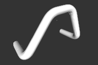
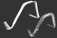
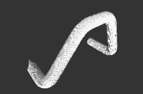
(a)	(b)	(c)	(d)

Figure 1: Different kinds of 3D tubular data: (a) input data obtained from full laser scan, (b) partial scans from one direction, (c) digital set of voxels and (d) height map.

More generally, classic medial axis extraction looks to be a potential solution for tubular shape analysis [8]. However such extraction may be sensitive to noise or to the presence of small defaults in the volumetric discrete object (like small hole). Fig. 2 shows some results obtained with different methods available from the implementation given in the authors survey. We can clearly see that small holes in the digital object significantly degrade the result. More recently, many advances came from the field of mesh processing with approaches based on mesh contraction [3, 20]. However, they are generally not adapted to surface with boundaries like the partial scan data of Fig. 1. In the same way, they are not simple to adapt to volumetric data like digital object made of voxels or height map. To process volumetric discrete objects, Gradient Vector Flow [24] was exploited by Hassouna and Farag in order to propose a robust skeleton curve extraction [11]. This method was also adapted to process gray values volumetric images used in virtual endoscopy [5]. In the field of discrete geometry we can mention a method which propose to specifically exploit 3D discrete tools to extract some medial axis on grey-level images [4]. To sum up approaches on medial axis, they are designed to process shapes defined as volumes, but they fail when processing open surfaces or partial samplings of the shape boundary. To process such data, we can refer to the work of Tagliasacchi et al. [21], who propose an algorithm based on surface normals. However the resulting quality depends on manual parameter tuning.

In this work, we propose a unified approach to the reconstruction and the geometric analysis of tubular objects obtained from various input data types: laser scans sampling the shape boundary with partial or complete data (Fig. 1 (a,b)), voxel sets sampling the shape (Fig. 1 (c)) or more specifically from height map data (Fig. 1 (c,d)). Potential applications of the latter datatype are numerous because of the increasing development of Kinect®-like devices. Our main contributions are first to propose a simple and automatic centerline extraction algorithm, which mainly relies on a surface normal accumulation image. Like other Hough transform based applications [7, 23], this algorithm can handle various types of input data. We also propose to extract geometric information along the tubular object, by segmenting it into rectilinear and toric parts. This is achieved with a 3D extension of a previous work on circular arc detection along 2D curves. In the following sections, we first introduce the new method of centerline detection, then we show how to reconstruct the tubular shape and decompose it into meaningful parts. We conclude with representative experiments showing the qualities of our method.

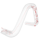
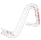
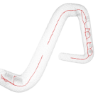
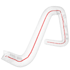
(a) thinning	(b) geometric	(c) potential field	(d) proposed
1 min 4s	0.5 s	3min	6s+3s

Figure 2: Skeleton extraction from three different methods presented in [8] with the implementation given by the authors. Our method is presented on the right.

2 Fast and Simple Centerline Extraction on 3D Tubular Object

In this section, we present centerline extraction algorithm based on surface normal accumulation. It consists in three main steps. First, we compute a 3D accumulation image, which counts for each voxel how many faces of input data have their normal vector pointing through the voxel (i). Depending on input data, normal vectors can be defined directly from the mesh faces or estimated by a more robust and accurate estimator (in particular if we process a digital object). Then a tracking algorithm (ii) extracts an approximate centerline by following local maxima in the accumulation image. Finally, to remove digitization effects due to the 3D discrete accumulation image, we optimize the position of center points (iii) by a gradient descent method.

2.1 Accumulation Images From Normal Vectors

The first algorithm requires as input a set of faces (a mesh or a digital surface), their associated normal vectors, and a 3D digital space (the 3D grid that will store the accumulated values). If the input object is a mesh, the gridstep of the digitization grid must be specified by the user. Depending on the awaited accuracy, a default gridstep can be chosen as the median size of mesh faces (with the face size defined as its longest edge). If the input object is a digital object or a heightmap, the digitization grid just matches their resolution. Besides, this algorithm requires as parameter some approximation of the tube radius $R$.

The whole algorithm is detailed in Algorithm 1. It outputs for each voxel the number of normal vectors going through it as well as a vector estimating the tube local main directions (i.e. the tangent to the centerline or equivalently the direction of minimal curvature along the tube boundary). Fig. 3 illustrates the main steps of the algorithm with the 3D directional scans, starting from the face origin $f_{k}$ in the direction of its normal vector $\overrightarrow{n_{k}}$ along a distance denoted accRadius (set to $R+\epsilon$ where $\epsilon$ is used to take into account possible small variations of the radius along the tube, see image (a) of Fig. 1). During the scan, the accumulation scores are stored for each visited voxel (image (b) of the same figure). The principal direction $\overrightarrow{p}$ of a voxel is also updated for each scan (image (c)). More precisely, if we denote by $\overrightarrow{n_{j}}$ and $\overrightarrow{n_{k}}$ the two last normal vectors intersecting a voxel $V$ for the scans $j$ and $k$, the principal direction $\overrightarrow{d_{k}}$ for the current scan is given by: $\overrightarrow{d_{k}}=\overrightarrow{d_{j}}+(\overrightarrow{n_{k}}\wedge\overrightarrow{n_{j}})$. In order to ignore non significant directions induced by near colinear vectors, we add a small constant (set by default to $0.1$) to filter the norm of the resulting vector $\overrightarrow{n_{k}}\wedge\overrightarrow{n_{j}}$.

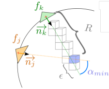
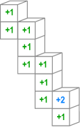
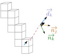
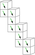
(a) directional scan	(b) accImage	(c) dirImage	(d) lastVectors

Figure 3: Illustration of Algorithm 1, which builds an accumulation image whose peaks match the centerline of the tubular shape.

Fig. 4 illustrates the computations made in Algorithm 1 for a mesh input data, and it shows the resulting accumulation image (image (c)) and vectors $\overrightarrow{n}$ orthogonal to the tube main direction $\overrightarrow{d}$. Since centerline extraction relies on these accumulation images, we evaluate the robustness of these images with various input surface types. The first row of Fig. 5 presents the resulting 3D accumulation images obtained on partial, noisy, digital or on small resolution mesh. In all these configurations, relative maximal values are indeed well located near the center of the tubular shape. A fixed threshold was applied in order to highlight the voxels with accumulation values close to maximal ones. Such voxels are drawn in black and for a particular selected voxel, we have highlighted their scanning origin faces with blue lines. All these results confirm the robustness of the proposed algorithm. We have therefore a solid basis for the tracking algorithm presented in the following part.

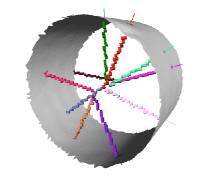
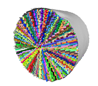
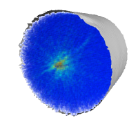
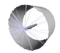
(a)	(b)	(c)	(d)

Figure 4: Illustration of accumulation images generated from surface normal vectors. Image (a) (resp. (b)) illustrates some (resp. all) scanning directions defined from mesh triangles. Image (c) illustrates the values obtained in the 3D accumulation image and (d) shows some voxels having accumulation score upper than a given threshold. In the last image we also display the set of faces contributing to the accumulation score.

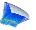
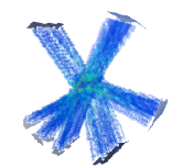
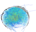
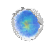
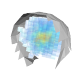
(a)	(b)	(c)	(d)	(e)
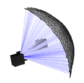
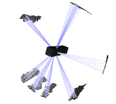
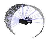
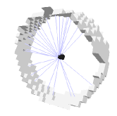
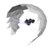
(f)	(g)	(h)	(i)	(j)

Figure 5: Experiment of the robustness of the surface normal accumulation algorithm applied on different types of input surface: on sector filtered mesh (a,f), on partial scan mesh (b,g), on noisy mesh (c,h), on digital surface (d,i), and on small resolution mesh (e,j).

Input : mesh // Triangular mesh of a tube

accRadius // Accumulation length from center of faces

minNorm = 0.1 // Minimum norm value

Ouput : accImage // Accumulation of normal vector number passing through a coordinate

dirImage // Cross product of all normals passing through a coordinate

maxAcc // Maximum number of normals passing through an (x,y,z) coordinate

maxPt // maxAcc coordinates

Variable : lastVectors // The last considered normal for each (x,y,z) coordinate

mainAxis // Vector contributing to the cross product of a directional vector

lastVectors = Image3D(mesh.dimensions())

maxAcc = 0

foreach face in mesh do

       currentPt = face.center

      normalVector = face.normalVector().normalized()

      while distance(currentPt, face.center) $<$ accRadius do

            

            if accImage[currentPt] != 0  then

                  

                  mainAxis = lastVectors[currentPt] $\times$ normalVector

                  if norm(mainAxis) $>$ minNorm then

                         dirImage[currentPt] += mainAxis*sign(mainAxis $\bullet$ dirImage[currentPt])

                  

            lastVectors[currentPt] = normalVector

            accImage[currentPt]++

            if accImage[currentPt] $>$ maxAcc then

                  

                  maxAcc = accImage[currentPt]

                  maxPt = currentPt

            

            currentPt += normalVector

      

Algorithm 1 accumulationFromNormalVectors : From position and normals of faces of an input mesh, this algorithm computes an accumulation image (accImage) by a directional scan starting from a face center in the direction of the face inward normal. It also outputs the image of vectors representing the local main axis direction of the tubular shape (dirImage).

2.2 Centerline Tracking from Image Accumulation

Even if the maximal values obtained in the previous part are well centered on the tubular object, a simple thresholding is not robust enough to extract directly the centerline. Furthermore it implies the manual adjustment of the threshold parameter. To illustrate this point, the image on the side shows different results obtained by choosing various threshold parameters $\sigma$. A too strict threshold implies disconnected points, while a less restrictive one produces a thick line with parasite voxels.

To better approach the centerline we propose to define a simple tracking algorithm exploiting the output of Algorithm 1, i.e. the accumulation image and the direction vectors image. As described in Algorithm 2, the main idea is to start from a point $C_{0}$ detected as a maximal accumulation value of the 3D accumulation image. Then, from a current point $C_{i}$ of the centerline, the algorithm determines next point $C_{i+1}$ as the point having maximal accumulation value in the 2D patch image $I_{patch}^{i}$ defined in the plane normal to the direction dirImage($C_{i}$) at distance trackStep (see Fig. 6 (a,b)).

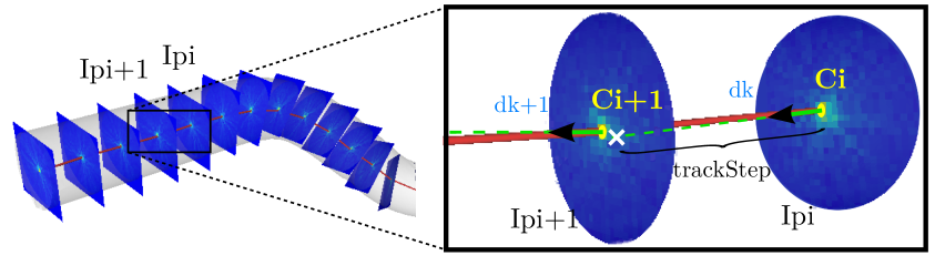
Figure 6: Tracking algorithm step. The patch $I_{patch}^{i+1}$ is generated from the maximum $C_{i}$ of $I_{patch}^{i}$ in the $\overrightarrow{d_{k}}$ direction at a trackStep distance before to localize the maximum $C_{i+1}$ of this new patch.

Input : accImage // Accumulation of normal vector number passing through a coordinate

dirImage // Cross product of all normals passing through a coordinate

accRadius // Accumulation length from center of faces

startPt, // Start point for tracking (must belong to the centerline)

trackInFront // True if tracking direction is in the startPt vector direction

trackStep // Distance between two consecutive centerline points

Output : centerline // Point set constituting the tube centerline

Variable : continueTracking // True if tracking can continue

patchSize // Dimension of the square patch

currentPt, previousPt // Considered point during an iteration

lastVect // Directional vector associated to previousPt

centerPatch // Patch center finding from currentPt

patchImageSize = 2 * aRadius ;

centerline = emptySet()

continueTracking = true

patchSize = 2 * accRadius

currentPt = startPt

lastVect = trackInFront ? dirImage( startPt ) : - dirImage( startPt )

previousPt = startPt - lastVect * trackStep

while continueTracking do

       centerline.append( currentPt )

      dirVect = dirImage[currentPt].normalized()

      if lastVect.dot(dirVect) $<0$ then

             dirVect = -dirVect

      

      continueTracking = isInsideTube( accImage, currentPt, previousPt, trackStep, $\pi/3$ )

      previousPt = currentPt

      // Defined the next image patch center point

      centerPatch = currentPt + ( dirVect * trackStep )

      if not accImage.domain().contains( centerPatch ) then

             break

      

      // Extract a 2D image of size 2 * accRadius from the 3D image accImage, centered on

       // centerPatch and directed along dirVect

       patchImage = extractPatch( accImage, centerPatch, dirVect, 2 * accRadius )

      maxCoords = getMaxCoords( patchImage )

      lastVect = dirVect

      previousPt = currentPt

      currentPt = patchSpaceToAccImageSpace( maxCoords)

return centerline

.

Algorithm 2 trackPatchCenter: tracking algorithm in one direction, given a starting point and an orientation.

2.3 Skeleton position optimization

Since the resulting tracking skeleton is embedded in a digital space, it suffers from digitization artefacts and is not perfectly centered within the input mesh. Moreover, depending on normal mesh quality, the tracking algorithm can potentially be influenced by perturbated normal directions, and may deviate from the expected centerline. Such perturbations can dramatically degrade the quality of upcoming geometric analysis, and hence impose some unwanted post processing tasks. To avoid such a difficulty, we propose to apply an optimization algorithm in order to obtain a perfectly centered spine line.

The idea is to model the quality of the current fitting by an error $E_{s}(C)$, defined as the sum of the squared difference between the known tube radius $R$ and the distance between the tube center $C$ and its associated input mesh points $M_{i}$. We wish to find the best position for center $C$ that minimizes this error. Otherwise said, we look for the circle of radius $R$ that best fits the data points $M_{i}$ in the least-square sense. Hence, the error is

$$E_{s}(C)=\sum_{i=0}^{N-1}{(\|\overrightarrow{CM_{i}}\|-R)^{2}}.$$ (1)

This minimization problem is easily solved by a gradient descent algorithm that follows the direction of steepest descent of the error. By simple derivation, its gradient is

$$\nabla E_{s}(C)=2\sum_{i=0}^{N-1}\frac{\overrightarrow{CM_{i}}}{\|\overrightarrow{CM_{i}}\|}{(R-\|\overrightarrow{CM_{i}}\|)}.$$ (2)

The gradient descent can also be interpreted as elastic forces acting on the center $C$ and pulling or pushing it in the direction of data according to the current distance. Then the minimization process applies at each step of the process the sum $\overrightarrow{f}$ of theses forces on $C$, giving with the notations of Fig. 7: $\overrightarrow{f}=\sum_{i=0}^{N}{\overrightarrow{P_{i}M_{i}}}$

By this way, at each step, the total error $E_{S}$ decrease and we iterate the process until convergence, i.e. the difference of errors between two iterations is below a fixed $\epsilon_{o}$.

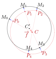
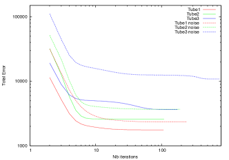
Figure 7: (left) Illustration of the process to optimize the centerline position (point $C$) with elastic forces (blue arrows). Each elastic force is attached to one point of the input mesh sector (a point $M_{i}$ represented in black) and oriented in the direction of the center of the virtual circle of center $S$. (right) evolution of the convergence speed in the optimization process.

Contrary to a simple average of neighborhood points, the optimization performs well even on partial mesh data, with missing parts or holes. Moreover, it is possible to ponder each force with its face area in order to better balance forces in presence of irregular sampling with variable density.

3 Reconstruction Results and Geometric Analysis

Reconstruction results. Several centerline extractions and tubular shape reconstructions are shown on Fig. 8. Our input dataset contains several types of metallic tubes numerized with different acquisition tools. In each case, the centerline is always well delineated without the need to tune a special parameter. When the input data is a complete or partial mesh, the normal is simply estimated as the cross product of face edges. When the input data is a digital object or a height map, we use the digital Voronoi Covariance Measure [9] to estimate the normal vector. Parameters of this estimator are easily set since we know the radius of the tubular object; they also have little influence on the result, since the accumulation image makes the process very robust. The running time was less than 30s for each experiment. As show on image (j) and (f), few places present reconstruction errors. Small errors may be found near bent areas. These errors are less related to the reconstruction method than to the physical shape under study, since the bending machine has deformed the tube at these places.

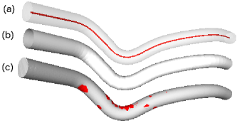
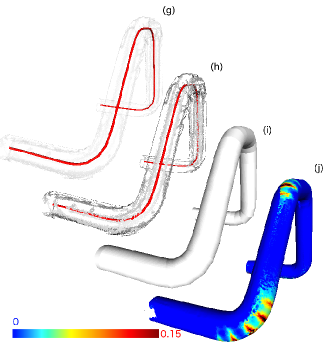
Full mesh	Partial mesh
$R=6$, t=6.23s, 151 444 faces	$R=6$, t=2.45s, 37 527 faces
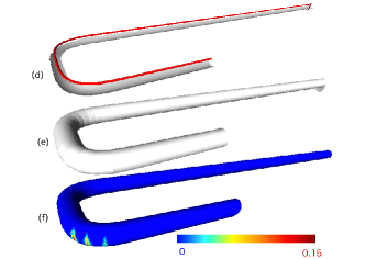
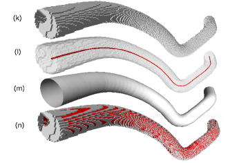
Reduced scaned area	Digital object
$R=6$, t=4.36s, 52 914 faces	$R=4.9$, t=6.91s, 60 768 faces
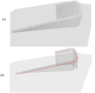
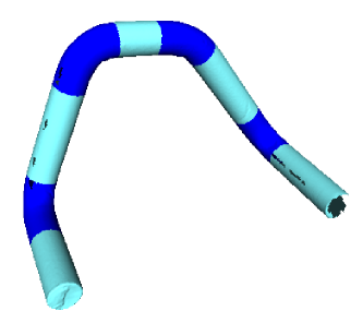
Height map	(q) straight (in light blue) and toric
$R=8$,t=22.33s, 645 450 faces	(in dark blue) segments.
	$R=6$, t=12.17s, 187 638 faces

Figure 8: Result of reconstruction from various input data types. Images (a,g,l,p) show the centerline by transparency through the input surface, (k) and (o) are some input surfaces. (b,e,i,m) images are the reconstructed tubes built from the centerlines. Images (j) and (f) show the local squared distance error between the reconstructed tube and the input shape. Image (q) illustrates the decomposition of a tube into rectilinear and toric parts. For all experiments, the tracking parameter and epsilon were set respectively to $R$ and 0.001. Running times correspond to executions on a MacBook computer with a 2,5 GHz Intel Core i7 processor.

(a) input polygonal curve	(b) Tangent space representation

Geometric analysis with 3D arc detection. We wish to segment the tubular shape into rectilinear and toric parts. This problem is equivalent to segmenting its centerline into 3D straight segments and 3D circular arcs. We thus extend to 3D a method presented by Nguyen et al. [18], which was designed to cut a 2D discrete curve into straight and circular pieces. It relies on properties of circular arcs in the tangent space representation that are inspired from Arkin [2] and Latecki [14]. The tangent space representation of a sequence of points $C=\{C_{i}\}_{i=0}^{n}$ is defined as follows :

Let $l_{i}$ be the length of segment $C_{i}C_{i+1}$ and $\alpha_{i}=\angle(\overrightarrow{C_{i-1}C_{i}},\overrightarrow{C_{i}C_{i+1}})$. Let us consider the transformation that associates $C$ with a polygon of $\mathbb{R}^{2}$ constituted by segments $T_{i2}T_{(i+1)1},T_{(i+1)1}T_{(i+1)2}$, $0\leq i<n$ (upper floating figure) with: $T_{02}=(0,0)$, $T_{i1}=(T_{(i-1)2}.x+l_{i-1},T_{(i-1)2}.y)$ for $i$ from $1$ to $n$, and $T_{i2}=(T_{i1}.x,T_{i1}.y+\alpha_{i})$ for $i$ from $1$ to $n-1$. Moreover, let $M=(M_{i})_{i=0}^{n-1}$ be the sequence of midpoints of segments $T_{i2}T_{(i+1)1}$ for $i$ from $0$ to $n-1$. The main idea of the arc detection method is that if $C$ is a polygon that approximates a circle or an arc of circle then $(M_{i})_{i=0}^{n-1}$ is a sequence of (approximately) co-linear points [18].

In our work, the sequence $(C_{i})_{i}$ of skeleton points obtained in Section 2.3 is considered and the representation of this sequence of points in the tangent space is computed. If the angles $\alpha_{k}$, for $k$ from $p$ to $q$, of consecutive points of $(C_{k})_{k=p}^{q}$ are close to $0$, these points belong to a straight line. Otherwise, the co-linearity of the corresponding midpoints $(M_{k})_{k=p}^{q}$ is tested in the tangent space by using an algorithm presented in  [18]. Fig. 8 (q) shows an example of tubular shape decomposition with this 3D variant of circular arc detection. Toric and rectilinear parts are correctly identified.

4 Conclusion and Discussion

A new efficient and simple method was presented to solve the problem of delineating the centerline of 3D tubular shapes, for various types of input data approximating its boundary: mesh, set of voxels or height map. The method is robust to missing parts in input data as well as perturbations: in these situations, it still returns accurately the centerline position. To achieve this, we have decomposed the process in three steps : 1) computing an accumulation map from faces and their normal vectors, 2) tracking of centerline through cross-section maximas of the accumulation map and 3) optimization of the centerline position by a better fitting of the model to the nearest faces along the centerline. The centerline was accurate enough to allow further geometric analysis. We have shown how to decompose the tubular shape into rectilinear and toric parts by a simple adaptation of a 2D circular arc detection algorithm. The hypothesis about constant radius parameter $R$ only influences the skeleton position optimization. This limitation could be resolved either by direct radius estimation from the accumulation image or by radius optimization during position optimization. This is left for future works. The whole process was implemented with the DGtal [1] framework and will soon be available in its companion DGtalTools.

5 Acknowledgments

The authors would like to thank the anonymous reviewers and Nicolas Passat for their many constructive comments, suggestions and references that really helped to improve this paper.

References

- [1] DGtal: Digital Geometry tools and algorithms library, http://libdgtal.org
- [2] Arkin, E., Chew, L., Huttenlocher, D., Kedem, K., Mitchell, J.: An efficiently computable metric for comparing polygonal shapes. TPAMI 13, 209–216 (1991)
- [3] Au, O.K.C., Tai, C.L., Chu, H.K., Cohen-Or, D., Lee, T.Y.: Skeleton Extraction by Mesh Contraction. In: ACM SIGGRAPH. pp. 44:1–44:10. ACM (2008)
- [4] Baja, G.S.d., Nyström, I., Borgefors, G.: Discrete 3d Tools Applied to 2d Grey-Level Images. In: ICIAP, pp. 229–236. No. 3617 in LNCS (2005)
- [5] Bauer, C., Bischof, H.: Extracting Curve Skeletons from Gray Value Images for Virtual Endoscopy. In: Dohi, T., Sakuma, I., Liao, H. (eds.) Medical Imaging and Augmented Reality, pp. 393–402. No. 5128 in Lecture Notes in Computer Science, Springer Berlin Heidelberg (2008)
- [6] Bauer, U., Polthier, K.: Generating parametric models of tubes from laser scans. Computer-Aided Design 41(10), 719–729 (Oct 2009)
- [7] Borrmann, D., Elseberg, J., Lingemann, K., Nüchter, A.: The 3d Hough Transform for plane detection in point clouds: A review and a new accumulator design. 3D Research 2(2), 1–13 (Nov 2011)
- [8] Cornea, N.D., Silver, D.: Curve-skeleton properties, applications, and algorithms. IEEE Transactions on Visualization and Computer Graphics 13, 530–548 (2007)
- [9] Cuel, L., Lachaud, J.O., Thibert, B.: Voronoi-based geometry estimator for 3d digital surfaces. In: DGCI. pp. 134–149. Springer (2014)
- [10] Goulette, F.: Automatic CAD modeling of industrial pipes from range images. In: 3-D Digital Imaging and Modeling, 1997. Proc.., ICRA. pp. 229–233 (1997)
- [11] Hassouna, M., Farag, A.: Variational Curve Skeletons Using Gradient Vector Flow. IEEE Transactions on Pattern Analysis and Machine Intelligence 31(12), 2257–2274 (Dec 2009)
- [12] Kirbas, C., Quek, F.: A review of vessel extraction techniques and algorithms. ACM Computing Surveys (CSUR) 36(2), 81–121 (2004)
- [13] Krähenbühl, A., Kerautret, B., Debled-Rennesson, I., Mothe, F., Longuetaud, F.: Knot Segmentation in 3d CT Images of Wet Wood. Pattern Recognition (2014)
- [14] Latecki, L., Lakamper, R.: Shape similarity measure based on correspondence of visual parts. IEEE Transactions on PAMI 22, 1185–1190 (2000)
- [15] Lee, I.K.: Curve reconstruction from unorganized points. Computer aided geometric design 17(2), 161–177 (2000)
- [16] Lee, I.K., Kim, K.J.: Shrinking: Another method for surface reconstruction. In: Geometric Modeling and Processing, 2004. Proceedings. pp. 259–266. IEEE (2004)
- [17] Lesage, D., Angelini, E.D., Bloch, I., Funka-Lea, G.: A review of 3d vessel lumen segmentation techniques: Models, features and extraction schemes. Medical Image Analysis 13(6), 819–845 (Dec 2009)
- [18] Nguyen, T.P., Debled-Rennesson, I.: Arc segmentation in linear time. In: 14th International Conference, CAIP, Seville, Spain. LNCS, vol. 6854, pp. 84–92 (2011)
- [19] Pare, P., Nagano, T., Coxson, H.: Airway imaging in disease: Gimmick or useful tool? Journal of Applied Physiology 113(4), 636–646 (2012)
- [20] Tagliasacchi, A., Alhashim, I., Olson, M., Zhang, H.: Mean curvature skeletons. In: Computer Graphics Forum. vol. 31, pp. 1735–1744. Wiley Online Library (2012)
- [21] Tagliasacchi, A., Zhang, H., Cohen-Or, D.: Curve skeleton extraction from incomplete point cloud. ACM Transactions on Graphics (TOG) 28(3), 71 (2009)
- [22] Tankyevych, O., Talbot, H., Passat, N., Musacchio, M., Lagneau, M.: Angiographic image analysis. In: Medical Image Processing, pp. 115–144. Springer (2011)
- [23] Tarsha-Kurdi, F., Landes, T., Grussenmeyer, P.: Hough-transform and extended ransac algorithms for automatic detection of 3d building roof planes from lidar data. In: ISPRS Workshop on Laser Scanning 2007 and SilviLaser 2007. vol. 36, pp. 407–412 (2007)
- [24] Xu, C., Prince, J.: Snakes, shapes, and gradient vector flow. IEEE Transactions on Image Processing 7(3), 359–369 (Mar 1998)