A new bijection relating $q$-Eulerian polynomials

Abstract

On the set of permutations of a finite set, we construct a bijection which maps the 3-vector of statistics $(\text{maj}-\text{exc},\text{des},\text{exc})$ to a 3-vector $(\text{maj}_{2},\widetilde{\text{des}_{2}},\text{inv}_{2})$ associated with the $q$-Eulerian polynomials introduced by Shareshian and Wachs in Chromatic quasisymmetric functions, arXiv:1405.4269(2014).

Notations

For all pair of integers $(n,m)$ such that $n<m$, the set $\{n,n+1,\ldots,m\}$ is indifferently denoted by $[n,m]$,$]n-1,m]$,$[n,m+1[$ or $]n-1,m+1[$.

The set of positive integers $\{1,2,3,\ldots\}$ is denoted by $\mathbb{N}_{>0}$.

For all integer $n\in\mathbb{N}_{>0}$, we denote by $[n]$ the set $[1,n]$ and by $\mathfrak{S}_{n}$ the set of the permutations of $[n]$. By abuse of notation, we assimilate every $\sigma\in\mathfrak{S}_{n}$ with the word $\sigma(1)\sigma(2)\ldots\sigma(n)$.

If a set $S=\{n_{1},n_{2},\ldots,n_{k}\}$ of integers is such that $n_{1}<n_{2}<\ldots<n_{k}$, we sometimes use the notation $S=\{n_{1}<n_{2}<\ldots<n_{k}\}$.

1 Introduction

Let $n$ be a positive integer and $\sigma\in\mathfrak{S}_{n}$. A descent (respectively exceedance point) of $\sigma$ is an integer $i\in[n-1]$ such that $\sigma(i)>\sigma(i+1)$ (resp. $\sigma(i)>i$). The set of descents (resp. exceedance points) of $\sigma$ is denoted by $\text{DES}(\sigma)$ (resp. $\text{EXC}(\sigma)$) and its cardinal by $\text{des}(\sigma)$ (resp. $\text{exc}(\sigma)$). The integers $\sigma(i)$ with $i\in\text{EXC}(\sigma)$ are called exceedance values of $\sigma$.

It is due to MacMahon [4] and Riordan [5] that

$$\sum\limits_{\sigma\in\mathfrak{S}_{n}}t^{\text{des}(\sigma)}=\sum\limits_{\sigma\in\mathfrak{S}_{n}}t^{\text{exc}(\sigma)}=A_{n}(t)$$

where $A_{n}(t)$ is the $n$-th Eulerian polynomial [1]. A statistic equidistributed with des or exc is said to be Eulerian. The statistic ides defined by $\text{ides}(\sigma)=\text{des}(\sigma^{-1})$ obviously is Eulerian.

The major index of a permutation $\sigma\in\mathfrak{S}_{n}$ is defined as

$$\text{maj}(\sigma)=\sum\limits_{i\in\text{DES}(\sigma)}i.$$

It is also due to MacMahon that

$$\sum\limits_{\sigma\in\mathfrak{S}_{n}}q^{\text{maj}(\sigma)}=\prod\limits_{i=1}^{n}\dfrac{1-q^{i}}{1-q}.$$

A statistic equidistributed with maj is said to be Mahonian. Among Mahonian statistics is the statistic inv, defined by $\text{inv}(\sigma)=|\text{INV}(\sigma)|$ where $\text{INV}(\sigma)$ is the set of inversions of a permutation $\sigma\in\mathfrak{S}_{n}$, i.e. the pairs of integers $(i,j)\in[n]^{2}$ such that $i<j$ and $\sigma(i)>\sigma(j)$.

In [6], the authors consider analogous versions of the above statistics : let $\sigma\in\mathfrak{S}_{n}$, the set of 2-descents (respectively 2-inversions) of $\sigma$ is defined as

$$\text{DES}_{2}(\sigma)=\{i\in[n-1],\sigma(i)>\sigma(i+1)+1\}$$

(resp.

$$\text{INV}_{2}(\sigma)=\{1\leq i<j\leq n,\sigma(i)=\sigma(j)+1\})$$

and its cardinal is denoted by $\text{des}_{2}(\sigma)$ (resp. $\text{inv}_{2}(\sigma)$).

It is easy to see that $\text{inv}_{2}(\sigma)=\text{ides}(\sigma)$. The 2-major index of $\sigma$ is defined as

$$\text{maj}_{2}(\sigma)=\sum\limits_{i\in\text{DES}_{2}(\sigma)}i.$$

By using quasisymmetric function techniques, the authors of [6] proved the equality

$$\sum_{\sigma\in\mathfrak{S}_{n}}x^{\text{maj}_{2}(\sigma)}y^{\text{inv}_{2}(\sigma)}=\sum_{\sigma\in\mathfrak{S}_{n}}x^{\text{maj}(\sigma)-\text{exc}(\sigma)}y^{\text{exc}(\sigma)}.$$ (1)

Similarly, by using the same quasisymmetric function method as in [6], the authors of [2] proved the equality

$$\sum\limits_{\sigma\in\mathfrak{S}_{n}}x^{\text{amaj}_{2}(\sigma)}y^{\widetilde{\text{asc}_{2}}(\sigma)}z^{\text{ides}(\sigma)}=\sum\limits_{\sigma\in\mathfrak{S}_{n}}x^{\text{maj}(\sigma)-\text{exc}(\sigma)}y^{\text{des}(\sigma)}z^{\text{exc}(\sigma)}$$ (2)

where $\text{asc}_{2}(\sigma)$ is the number of 2-ascents of a permutation $\sigma\in\mathfrak{S}_{n}$, i.e. the elements of the set $\text{ASC}_{2}(\sigma)=\{i\in[n-1],\sigma(i)<\sigma(i+1)+1\}$, which rises the statistic $\text{amaj}_{2}$ defined by

$$\text{amaj}_{2}(\sigma)=\sum\limits_{i\in\text{ASC}_{2}(\sigma)}i,$$

and where

$$\widetilde{\text{asc}_{2}}(\sigma)=\begin{cases}\text{asc}_{2}(\sigma)&\text{if $\sigma(1)=1$,}\\ \text{asc}_{2}(\sigma)+1&\text{if $\sigma(1)\neq 1$.}\end{cases}$$

Definition 1.1.

Let $\sigma\in\mathfrak{S}_{n}$. We consider the smallest $2$-descent $d_{2}(\sigma)$ of $\sigma$ such that $\sigma(i)=i$ for all $i\in[d_{2}(\sigma)-1]$ (if there is no such $2$-descent, we define $d_{2}(\sigma)$ as $0$ and $\sigma(0)$ as $n+1$).

Now, let $d_{2}^{\prime}(\sigma)>d_{2}(\sigma)$ be the smallest $2$-descent of $\sigma$ greater than $d_{2}(\sigma)$ (if there is no such $2$-descent, we define $d_{2}^{\prime}(\sigma)$ as $n$).

We define an inductive property $\mathcal{P}(d_{2}(\sigma))$ by :

1. $\sigma(d_{2}(\sigma))<\sigma(i)$ for all $(i,j)\in\text{INV}_{2}(\sigma)$ such that $d_{2}(\sigma)<i<d_{2}^{\prime}(\sigma)$;

2. if $(d_{2}^{\prime}(\sigma),j)\in\text{INV}_{2}(\sigma)$ for some $j$, then either $\sigma(d_{2}(\sigma))<\sigma(d_{2}^{\prime}(\sigma))$, or $d_{2}^{\prime}(\sigma)$ has the property $\mathcal{P}(d_{2}^{\prime}(\sigma))$ (where the role of $d_{2}(\sigma)$ is played by $d_{2}^{\prime}(\sigma)$ and that of $d_{2}^{\prime}(\sigma)$ by $d_{2}^{\prime\prime}(\sigma)$ where $d_{2}^{\prime\prime}(\sigma)>d_{2}^{\prime}(\sigma)$ is the smallest $2$-descent of $\sigma$ greater than $d_{2}^{\prime}(\sigma)$, defined as $n$ if there is no such $2$-descent).

This property is well-defined because $(n,j)\not\in\text{INV}_{2}(\sigma)$ for all $j\in[n]$.

Finally, we define a statistic $\widetilde{\text{des}_{2}}$ by :

$$\widetilde{\text{des}_{2}}(\sigma)=\begin{cases}\text{des}_{2}(\sigma)&\text{if the property $\mathcal{P}(d_{2}(\sigma))$ is true,}\\ \text{des}_{2}(\sigma)+1&\text{otherwise.}\end{cases}$$

In the present paper, we prove the following theorem.

Theorem 1.2.

There exists a bijection $\varphi:\mathfrak{S}_{n}\rightarrow\mathfrak{S}_{n}$ such that

$$(\text{maj}_{2}(\sigma),\widetilde{\text{des}_{2}}(\sigma),\text{inv}_{2}(\sigma))=(\text{maj}(\varphi(\sigma))-\text{exc}(\varphi(\sigma)),\text{des}(\varphi(\sigma)),\text{exc}(\varphi(\sigma))).$$

As a straight corollary of Theorem 1.2, we obtain the equality

$$\sum\limits_{\sigma\in\mathfrak{S}_{n}}x^{\text{maj}_{2}(\sigma)}y^{\widetilde{\text{des}_{2}}(\sigma)}z^{\text{inv}_{2}(\sigma)}=\sum\limits_{\sigma\in\mathfrak{S}_{n}}x^{\text{maj}(\sigma)-\text{exc}(\sigma)}y^{\text{des}(\sigma)}z^{\text{exc}(\sigma)}$$ (3)

which implies Equality (1).

The rest of this paper is organised as follows.

In Section 2, we introduce two graphical representations of a given permutation so as to highlight either the statistic $(\text{maj}-\text{exc},\text{des},\text{exc})$ or $(\text{maj}_{2},\widetilde{\text{des}_{2}},\text{inv}_{2})$. Practically speaking, the bijection $\varphi$ of Theorem 1.2 will be defined by constructing one of the two graphical representations of $\varphi(\sigma)$ for a given permutation $\sigma\in\mathfrak{S}_{n}$.

We define $\varphi$ in Section 3.

In Section 4, we prove that $\varphi$ is bijective by constructing $\varphi^{-1}$.

2 Graphical representations

2.1 Linear graph

Let $\sigma\in\mathfrak{S}_{n}$. The linear graph of $\sigma$ is a graph whose vertices are (from left to right) the integers $\sigma(1),\sigma(2),\ldots,\sigma(n)$ aligned in a row, where every $\sigma(k)$ (for $k\in\text{DES}_{2}(\sigma)$) is boxed, and where an arc of circle is drawn from $\sigma(i)$ to $\sigma(j)$ for every $(i,j)\in\text{INV}_{2}(\sigma)$.

For example, the permutation $\sigma=34251\in\mathfrak{S}_{5}$ (such that $(\text{maj}_{2}(\sigma),\widetilde{\text{des}_{2}}(\sigma),\text{inv}_{2}(\sigma))=\leavevmode\nobreak\ (6,3,2)$) has the linear graph depicted in Figure 1.

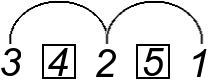
Figure 1: Linear graph of $\sigma=34251\in\mathfrak{S}_{5}$.

2.2 Planar graph

Let $\tau\in\mathfrak{S}_{n}$. The planar graph of $\tau$ is a graph whose vertices are the integers $1,2,...,n$, organized in ascending and descending slopes (the height of each vertex doesn’t matter) such that the $i$-th vertex (from left to right) is the integer $\tau(i)$, and where every vertex $\tau(i)$ with $i\in\text{EXC}(\tau)$ is encircled.

For example, the permutation $\tau=32541\in\mathfrak{S}_{5}$ (such that $(\text{maj}(\tau)-\text{exc}(\tau),\text{des}(\tau),\text{exc}(\tau))=(6,3,2))$ has the planar graph depicted in Figure 2.

Figure 2: Planar graph of $\tau=32541\in\mathfrak{S}_{5}$.

3 Definition of the map $\varphi$ of Theorem 1.2

Let $\sigma\in\mathfrak{S}_{n}$. We set $(r,s)=(\text{des}_{2}(\sigma),\text{inv}_{2}(\sigma))$, and

$$\text{DES}_{2}(\sigma) =\left\{d_{2}^{k}(\sigma),k\in[r]\right\},$$

$$\text{INV}_{2}(\sigma) =\{(i_{l}(\sigma),j_{l}(\sigma)),l\in[s]\}$$

with $d_{2}^{k}(\sigma)<d_{2}^{k+1}(\sigma)$ for all $k$ and $i_{l}(\sigma)<i_{l+1}(\sigma)$ for all $l$.

We intend to define $\varphi(\sigma)$ by constructing its planar graph. To do so, we first construct (in Subsection 3.1) a graph $\mathcal{G}(\sigma)$ made of $n$ circles or dots organized in ascending or descending slopes such that two consecutive vertices are necessarily in a same descending slope if the first vertex is a circle and the second vertex is a dot. Then, in Subsection 3.2, we label the vertices of this graph with the integers $1,2,\ldots,n$ in such a way that, if $y_{i}$ is the label of the $i$-th vertex $v_{i}(\sigma)$ (from left to right) of $\mathcal{G}(\sigma)$ for all $i\in[n]$, then :

1. $y_{i}<y_{i+1}$ if and only if $v_{i}$ and $v_{i+1}$ are in a same ascending slope;

2. $y_{i}>i$ if and only if $v_{i}$ is a circle.

The permutation $\tau=\varphi(\sigma)$ will then be defined as $y_{1}y_{2}\ldots y_{n}$, i.e. the permutation whose planar graph is the labelled graph $\mathcal{G}(\sigma)$.

With precision, we will obtain

$$\tau\left(\text{EXC}(\tau)\right)=\{j_{k}(\sigma),k\in[s]\}$$

(in particular $\text{exc}(\tau)=s=\text{inv}_{2}(\sigma)$), and

$$\text{DES}(\tau)=\begin{cases}\{d^{k}(\sigma),k\in[1,r]\}\text{ if $\widetilde{\text{des}_{2}}(\sigma)=r$},\\ \{d^{k}(\sigma),k\in[0,r]\}\text{ if $\widetilde{\text{des}_{2}}(\sigma)=r+1$}\end{cases}$$

for integers $0\leq d^{0}(\sigma)<d^{1}(\sigma)<\ldots<d^{r}(\sigma)\leq n$ (with $d^{0}(\sigma)=0\Leftrightarrow\widetilde{\text{des}_{2}}(\sigma)=\text{des}_{2}(\sigma)$) defined by

$$d^{k}(\sigma)=d_{2}^{k}(\sigma)+c_{k}(\sigma)$$

(with $d_{2}^{0}(\sigma):=0$) where $(c_{k}(\sigma))_{k\in[0,r]}$ is a sequence defined in Subsection 3.1 such that $\sum_{k}c_{k}(\sigma)=\text{inv}_{2}(\sigma)=\text{exc}(\tau)$. Thus, we will obtain $\text{des}(\tau)=\widetilde{\text{des}_{2}}(\sigma)$ and $\text{maj}(\tau)=\text{maj}_{2}(\sigma)+\text{exc}(\tau)$.

3.1 Construction of the unlabelled graph $\mathcal{G}(\sigma)$

We set $\left(d_{2}^{0}(\sigma),\sigma(d_{2}^{0}(\sigma))\right)=(0,n+1)$ and $\left(d_{2}^{r+1}(\sigma),\sigma(n+1)\right)=(n,0)$.

For all $k\in[r]$, we define the top $t_{k}(\sigma)$ of the 2-descent $d_{2}^{k}(\sigma)$ as

$$t_{k}(\sigma)=\min\{d_{2}^{l}(\sigma),1\leq l\leq k,d_{2}^{l}(\sigma)=d_{2}^{k}(\sigma)-(k-l)\},$$ (4)

in other words $t_{k}(\sigma)$ is the smallest 2-descent $d_{2}^{l}(\sigma)$ such that the 2-descents $d_{2}^{l}(\sigma),d_{2}^{l+1}(\sigma),\ldots,d_{2}^{k}(\sigma)$ are consecutive integers.

The following algorithm provides a sequence $(c^{0}_{k}(\sigma))_{k\in[0,r]}$ of nonnegative integers.

Algorithm 3.1.

Let $I_{r}(\sigma)=\text{INV}_{2}(\sigma)$. For $k$ from $r=\text{des}_{2}(\sigma)$ down to $0$, we consider the set $S_{k}(\sigma)$ of sequences $(i_{k_{1}}(\sigma),i_{k_{2}}(\sigma),\ldots,i_{k_{m}}(\sigma))$ such that :

1. $(i_{k_{p}}(\sigma),j_{k_{p}}(\sigma))\in I_{k}(\sigma)$ for all $p\in[m]$;

2. $t_{k}(\sigma)\leq i_{k_{1}}(\sigma)<i_{k_{2}}(\sigma)<\ldots<i_{k_{m}}(\sigma)$;

3. $\sigma(i_{k_{1}}(\sigma))<\sigma(i_{k_{2}}(\sigma))<\ldots<\sigma(i_{k_{m}}(\sigma))$.

The length of such a sequence is defined as $l=\sum_{p=1}^{m}n_{p}$ where $n_{p}$ is the number of consecutive 2-inversions whose beginning is $i_{k_{p}}$, i.e. the maximal number $n_{p}$ of 2-inversions $(i_{k_{p}^{1}}(\sigma),j_{k_{p}^{1}}(\sigma)),(i_{k_{p}^{2}}(\sigma),j_{k_{p}^{2}}(\sigma)),\ldots,(i_{k^{n_{p}}_{p}}(\sigma),j_{k^{n_{p}}_{p}}(\sigma))$ such that $k^{1}_{p}=k_{p}$ and $j_{k^{i}_{p}}(\sigma)=i_{k^{i+1}_{p}}(\sigma)$ for all $i$. If $I_{k}(\sigma)\neq\emptyset$, we consider the sequence $(i_{k^{max}_{1}}(\sigma),i_{k^{max}_{2}}(\sigma),\ldots,i_{k^{max}_{m}}(\sigma))\in I_{k}(\sigma)$ whose length $l^{max}=\sum_{p=1}^{m}n_{p}^{max}$ is maximal and whose elements $i_{k^{max}_{1}}(\sigma),i_{k^{max}_{2}}(\sigma),\ldots,i_{k^{max}_{m}}(\sigma)$ also are maximal (as integers). Then,

• if $I_{k}(\sigma)\neq\emptyset$, we set $c^{0}_{k}(\sigma)=l^{max}$ and

  $$I_{k-1}(\sigma)=I_{k}(\sigma)\backslash\left(\cup_{p=1}^{m}\{(i_{k^{max}_{i}}(\sigma),j_{k^{max}_{i}}(\sigma)),i\in[n_{p}^{max}]\}\right);$$

• else we set $c_{k}^{0}(\sigma)=0$ and $I_{k-1}(\sigma)=I_{k}(\sigma)$.

Example 3.2.

Consider the permutation $\sigma=549321867\in\mathfrak{S}_{9}$, with $\text{DES}_{2}(\sigma)=\{3,7\}$ and $I_{2}(\sigma)=\text{INV}_{2}(\sigma)=\{(1,2),(2,4),(3,7),(4,5),(5,6),(7,9)\}$. In Figure 3 are depicted the $\text{des}_{2}(\sigma)+1=3$ steps $k\in\{2,1,0\}$ (at each step, the 2-inversions of the maximal sequence are drawed in red then erased at the following step) :

Figure 3: Computation of $(c^{0}_{k}(\sigma))_{k\in[0,\text{des}_{2}(\sigma)]}$ for $\sigma=549321867\in\mathfrak{S}_{9}$.

• $k=2$ : there is only one legit sequence $(i_{k_{1}}(\sigma))=(7)$, whose length is $l=n_{1}=1$. We set $c^{0}_{2}(\sigma)=1$ and $I_{1}(\sigma)=I_{2}(\sigma)\backslash\{(7,9)\}$.

• $k=1$ : there are three legit sequences $(i_{k_{1}}(\sigma))=(3)$ (whose length is $l=n_{1}=1$) then $(i_{k_{1}}(\sigma))=(4)$ (whose length is $l=n_{1}=2$) and $(i_{k_{1}}(\sigma))=(5)$ (whose length is $l=n_{1}=1$). The maximal sequence is the second one, hence we set $c^{0}_{1}(\sigma)=2$ and $I_{0}(\sigma)=I_{1}(\sigma)\backslash\{(4,5),(5,6)\}$.

• $k=0$ : there are three legit sequences $(i_{k_{1}}(\sigma),i_{k_{2}}(\sigma))=(1,3)$ (whose length is $l=n_{1}+n_{2}=2+1=3$) then $(i_{k_{1}}(\sigma),i_{k_{2}}(\sigma))=(2,3)$ (whose length is $l=n_{1}+n_{2}=1+1=2$) and $(i_{k_{1}}(\sigma))=(3)$ (whose length is $l=n_{1}=1$). The maximal sequence is the first one, hence we set $c^{0}_{0}(\sigma)=3$ and $I_{-1}(\sigma)=I_{0}(\sigma)\backslash\{(1,2),(2,4),(3,7)\}=\emptyset$.

Lemma 3.3.

The sum $\sum_{k}c^{0}_{k}(\sigma)$ equals $\text{inv}_{2}(\sigma)$ (i.e. $I_{-1}(\sigma)=\emptyset$) and, for all $k\in[0,r]=[0,\text{des}_{2}(\sigma)]$, we have $c^{0}_{k}(\sigma)\leq d_{2}^{k+1}(\sigma)-d_{2}^{k}(\sigma)$ with equality only if $c^{0}_{k+1}(\sigma)>\leavevmode\nobreak\ 0$ (where $c^{0}_{r+1}(\sigma)$ is defined as $0$).

Proof. With precision, we show by induction that, for all $k\in\{\text{des}_{2}(\sigma),\ldots,1,0\}$, the set $I_{k-1}(\sigma)$ contains no 2-inversion $(i,j)$ such that $d_{2}^{k}(\sigma)<i$. For $k=0$, it will mean $I_{-1}(\sigma)=\emptyset$ (recall that $d_{2}^{0}(\sigma)$ has been defined as $0$).

$\star$ If $k=\text{des}_{2}(\sigma)=r$, the goal is to prove that $c^{0}_{r}(\sigma)<n-d_{2}^{r}(\sigma)$. Suppose there exists a sequence $(i_{k_{1}}(\sigma),i_{k_{2}}(\sigma),\ldots,i_{k_{m}}(\sigma))$ of length $c^{0}_{r}(\sigma)\geq n-d_{2}^{r}(\sigma)$ with $t_{r}(\sigma)\leq i_{k_{1}}(\sigma)<i_{k_{2}}(\sigma)<\ldots<i_{k_{m}}(\sigma)$. In particular, there exist $c^{0}_{r}(\sigma)\leavevmode\nobreak\ \geq\leavevmode\nobreak\ n-d_{2}^{r}(\sigma)$ 2-inversions $(i,j)$ such that $d_{2}^{r}(\sigma)<j$, which forces $c^{0}_{r}(\sigma)$ to equal $n-d_{2}^{r}(\sigma)$ and every $j>d_{2}^{r}(\sigma)$ to be the arrival of a 2-inversion $(i,j)$ such that $t_{r}(\sigma)\leq i$. In particular, this is true for $j=d_{2}^{r}(\sigma)+1$, which is absurd because $\sigma(i)\geq\sigma\left(d_{2}^{r}(\sigma)\right)>\sigma\left(d_{2}^{r}(\sigma)+1\right)+1$ for all $i\in[t_{r}(\sigma),d_{2}^{r}(\sigma)]$. Therefore $c^{0}_{r}(\sigma)<n-d_{2}^{r}(\sigma)$. Also, it is easy to see that every $i>d_{2}^{r}(\sigma)$ that is the beginning of a 2-inversion $(i,j)$ necessarily appears in the maximal sequence $\left(i_{k^{max}_{1}}(\sigma),i_{k^{max}_{2}}(\sigma),\ldots,i_{k^{max}_{m}}(\sigma)\right)$ whose length defines $c^{0}_{r}(\sigma)$, hence $(i,j)\not\in I_{r-1}(\sigma)$.

$\star$ Now, suppose that $c^{0}_{k}(\sigma)\leq d_{2}^{k+1}(\sigma)-d_{2}^{k}(\sigma)$ for some $k\in[\text{des}_{2}(\sigma)]$ with equality only if $c^{0}_{k+1}(\sigma)>0$, and that no 2-inversion $(i,j)$ with $d_{2}^{k}(\sigma)<i$ belongs to $I_{k-1}(\sigma)$.

If $t_{k-1}(\sigma)=t_{k}(\sigma)$ (i.e., if $d_{2}^{k-1}(\sigma)=d_{2}^{k}(\sigma)-1$), since $I_{k-1}(\sigma)$ does not contain any 2-inversion $(i,j)$ with $d_{2}^{k}(\sigma)<i$, then $c^{0}_{k-1}(\sigma)\leq 1=d_{2}^{k}(\sigma)-d_{2}^{k-1}(\sigma)$. Moreover, if $c^{0}_{k-1}(\sigma)=1$, then there exists a 2-inversion $(i,j)\in I_{k-1}(\sigma)\subset I_{k}(\sigma)$ such that $i\in[t_{k-1}(\sigma),d_{2}^{k}(\sigma)]$. Consequently $(i)$ was a legit sequence for the computation of $c^{0}_{k}(\sigma)$ at the previous step (because $t_{k}(\sigma)=t_{k-1}(\sigma)$), which implies $c^{0}_{k}(\sigma)$ equals at least the length of $(i)$. In particular $c^{0}_{k}(\sigma)>0$.

Else, consider a sequence $(i_{k_{1}}(\sigma),i_{k_{2}}(\sigma),\ldots,i_{k_{m}}(\sigma))$ that fits the three conditions of Algorithm 3.1 at the step $k-1$. In particular $t_{k-1}(\sigma)\leq i_{k_{1}}(\sigma)$. Also $i_{k_{m}}(\sigma)\leq d_{2}^{k}(\sigma)$ by hypothesis. Since $\sigma(i_{k_{p}}(\sigma))<\sigma(i_{k_{p+1}}(\sigma))$ for all $p$, and since $\sigma(t_{k-1}(\sigma))>\sigma(t_{k-1}(\sigma)+1)>\ldots>\sigma\left(d_{2}^{k-1}(\sigma)\right)>\sigma\left(d_{2}^{k-1}(\sigma)+1\right)$, then only one element of the set $[t_{k-1}(\sigma),d_{2}^{k-1}(\sigma)+1]$ may equal $i_{k_{p}}(\sigma)$ for some $p\in[m]$. Thus, the length $l$ of the sequence verifies $l\leq d_{2}^{k}(\sigma)-d_{2}^{k-1}(\sigma)$, with equality only if $i_{k_{m}}(\sigma)=d_{2}^{k}(\sigma)$ (which implies $c^{0}_{k}(\sigma)>0$ as in the previous paragraph). In particular, this is true for $l=c^{0}_{k-1}(\sigma)$.

Finally, as for $k=\text{des}_{2}(\sigma)$, every $i\in[d_{2}^{k-1}(\sigma)+1,d_{2}^{k}(\sigma)]$ that is the beginning of a 2-inversion $(i,j)$ necessarily appears in the maximal sequence $\left(i_{k^{max}_{1}}(\sigma),i_{k^{max}_{2}}(\sigma),\ldots,i_{k^{max}_{m}}(\sigma)\right)$ whose length defines $c^{0}_{k-1}(\sigma)$, hence $(i,j)\not\in I_{k-2}(\sigma)$.

So the lemma is true by induction. ∎

Definition 3.4.

We define a graph $\mathcal{G}^{0}(\sigma)$ made of circles and dots organised in ascending or descending slopes, by plotting :

• for all $k\in[0,r]$, an ascending slope of $c_{k}^{0}(\sigma)$ circles such that the first circle has abscissa $d_{2}^{k}(\sigma)+1$ and the last circle has abscissa $d_{2}^{k}(\sigma)+c_{k}^{0}(\sigma)$ (if $c_{k}^{0}(\sigma)=0$, we plot nothing). All the abscissas are distinct because

  $$d_{2}^{0}(\sigma)+c_{0}<d_{2}^{1}(\sigma)+c_{1}<\ldots<d_{2}^{r}(\sigma)+c_{r}$$

  in view of Lemma 3.3;

• dots at the remaining $n-s=n-\text{inv}_{2}(\sigma)$ abscissas from $1$ to $n$, in ascending and descending slopes with respect to the descents and ascents of the word $\omega(\sigma)$ defined by

  $$\omega(\sigma)=\sigma(u_{1}(\sigma))\sigma(u_{2}(\sigma))\ldots\sigma(u_{n-s}(\sigma))$$ (5)

  where

  $$\{u_{1}(\sigma)<u_{2}(\sigma)<\ldots<u_{n-s}(\sigma)\}:=\mathfrak{S}_{n}\backslash\{i_{1}(\sigma)<i_{2}(\sigma)<\ldots<i_{s}(\sigma)\}.$$

Example 3.5.

The permutation $\sigma_{0}=425736981\in\mathfrak{S}_{9}$ (with $\text{DES}_{2}(\sigma_{0})=\{1,4,8\}$ and $\text{INV}_{2}(\sigma_{0})=\{(1,5),(2,9),(4,6),(7,8)\}$), which yields the sequence $(c^{0}_{k}(\sigma_{0}))_{k\in[0,3]}=(1,1,2,0)$ (see Figure 4 where all the 2-inversions involved in the computation of a same $c^{0}_{k}(\sigma_{0})$ are drawed in a same color) and the word $\omega(\sigma_{0})=53681$, provides the unlabelled graph $\mathcal{G}^{0}(\sigma_{0})$ depicted in Figure 5.

Figure 4: $(c^{0}_{k}(\sigma_{0}))_{k\in[0,3]}=({\color[rgb]{1,0,0}1},{\color[rgb]{0,1,0}1},{\color[rgb]{0,0,1}2},0).$

Figure 5: Graph $\mathcal{G}^{0}(\sigma_{0})$.

The following lemma is easy.

Lemma 3.6.

For all $i\in[n]$, if the $i$-th vertex (from left to right) $v_{i}^{0}(\sigma)$ of $\mathcal{G}^{0}(\sigma)$ is a dot and if $i$ is a descent of $\mathcal{G}^{0}(\sigma)$ (i.e., if $v_{i}^{0}(\sigma)$ and $v_{i+1}^{0}(\sigma)$ are two dots in a same descending slope) whereas $i\not\in\text{DES}_{2}(\sigma)$, let $k_{i}$ such that

$$d_{2}^{k_{i}}(\sigma)\leavevmode\nobreak\ +\leavevmode\nobreak\ c^{0}_{k_{i}}(\sigma)\leavevmode\nobreak\ <\leavevmode\nobreak\ i<\leavevmode\nobreak\ d_{2}^{k_{i}+1}(\sigma)$$

and let $p\in[n-s]$ such that $v_{i}^{0}(\sigma)$ is the $p$-th dot (from left to right) of $\mathcal{G}^{0}(\sigma)$. Then :

1. $u_{p}(\sigma)$ is the greatest integer $u<d_{2}^{k_{i}+1}(\sigma)$ that is not the beginning of a 2-inversion of $\sigma$;

2. $u_{p+1}(\sigma)$ is the smallest integer $u>d_{2}^{k_{i}+1}(\sigma)$ that is not a 2-descent or the beginning of a 2-inversion of $\sigma$;

3. $c^{0}_{k}(\sigma)>0$ for all $k$ such that $d_{2}^{k_{i}+1}(\sigma)\leq d_{2}^{k}(\sigma)\leq u_{p+1}(\sigma)$.

In particular $c^{0}_{k_{i}+1}(\sigma)>0$.

Lemma 3.6 motivates the following definition.

Definition 3.7.

For $i$ from $1$ to $n-1$, let $k_{i}\in[0,r]$ such that

$$d_{2}^{k_{i}}(\sigma)\leavevmode\nobreak\ +\leavevmode\nobreak\ c^{0}_{k_{i}}(\sigma)\leavevmode\nobreak\ <\leavevmode\nobreak\ i<\leavevmode\nobreak\ d_{2}^{k_{i}+1}(\sigma).$$

If $i$ fits the conditions of Lemma 3.6, then we define a sequence $(c^{i}_{k}(\sigma))_{k\in[0,r]}$ by

$$c^{i}_{k_{i}}(\sigma) =c^{i-1}_{k_{i}}(\sigma)+1,$$

$$c^{i}_{k_{i}+1}(\sigma) =c^{i-1}_{k_{i}+1}(\sigma)-1,$$

$$c^{i}_{k}(\sigma) =c^{i-1}_{k}(\sigma)\text{ for all $k\not\in\{k_{i},k_{i}+1\}$.}$$

Else, we define $(c^{i}_{k}(\sigma))_{k\in[0,r]}$ as $(c^{i-1}_{k}(\sigma))_{k\in[0,r]}$.

The final sequence $(c^{n}_{k}(\sigma))_{k\in[0,r]}$ is denoted by

$$(c_{k}(\sigma))_{k\in[0,r]}.$$

By construction, and from Lemma 3.3, the sequence $(c_{k}(\sigma))_{k\in[0,r]}$ has the same properties as $(c^{0}_{k}(\sigma))_{k\in[0,r]}$ detailed in Lemma 3.3.

Consequently, we may define an unlabelled graph

$$\mathcal{G}(\sigma)$$

by replacing $(c^{0}_{k}(\sigma))_{k\in[0,r]}$ with $(c_{k}(\sigma))_{k\in[0,r]}$ in Definition 3.4.

Example 3.8.

In the graph $\mathcal{G}^{0}(\sigma)$ depicted in Figure 5 where $\sigma_{0}=425736981\in\mathfrak{S}_{9}$, we can see that the dot $v_{3}^{0}(\sigma_{0})$ is a descent whereas $3\not\in\text{DES}_{2}(\sigma_{0})$, hence, from the sequence $(c^{0}_{k}(\sigma_{0}))_{k\in[0,3]}=(1,1,2,0)$, we compute $(c_{k}(\sigma_{0}))_{k\in[0,3]}=(1,2,1,0)$ and we obtain the graph $\mathcal{G}(\sigma_{0})$ depicted in Figure 6.

Figure 6: Graph $\mathcal{G}(\sigma_{0})$.

Let $v_{1}(\sigma),v_{2}(\sigma),\ldots,v_{n}(\sigma)$ be the $n$ vertices of $\mathcal{G}(\sigma)$ from left to right.

By construction, the descents of the unlabelled graph $\mathcal{G}(\sigma)$ (i.e., the integers $i\in[n-1]$ such that $v_{i}(\sigma)$ and $v_{i+1}(\sigma)$ are in a same descending slope) are the integers

$$d^{k}(\sigma)=d_{2}^{k}(\sigma)+c_{k}(\sigma)$$

for all $k\in[0,r]$.

3.2 Labelling of the graph $\mathcal{G}(\sigma)$

3.2.1 Labelling of the circles

We intend to label the circles of $\mathcal{G}(\sigma)$ with the integers

$$j_{1}(\sigma),j_{2}(\sigma),\ldots,j_{s}(\sigma).$$

Algorithm 3.9.

For all $i\in[n]$, if the vertex $v_{i}(\sigma)$ is a circle (hence $i<n$), we label it first with the set

$$[i+1,n]\cap\{j_{1}(\sigma),j_{2}(\sigma),\ldots,j_{s}(\sigma)\}.$$

Afterwards, if a circle $v_{i}(\sigma)$ is found in a descending slope such that there exists a quantity of $a$ circles above $v_{i}(\sigma)$, and in an ascending slope such that there exists a quantity of $b$ circles above $v_{i}(\sigma)$, then we remove the $a+b$ greatest integers from the current label of $v_{i}(\sigma)$ (this set necessarily had at least $a+b+1$ elements) and the smallest integer from every of the $a+b$ labels of the $a+b$ circles above $v_{i}(\sigma)$ in the two related slopes. At the end of this step, if an integer $j_{k}(\sigma)$ appears in only one label of a circle $v_{i}(\sigma)$, then we replace the label of $v_{i}(\sigma)$ with $j_{k}(\sigma)$.

Finally, we replace every label that is still a set by the unique integer it may contain with respect to the order of the elements in the sequence

$$(j_{1}(\sigma),j_{2}(\sigma),\ldots,j_{s}(\sigma))$$

(from left to right).

Example 3.10.

For $\sigma_{0}=425736981$ (see Figure 4) whose graph $\mathcal{G}(\sigma_{0})$ is depicted in Figure 6, we have $s=\text{inv}_{2}(\sigma)=4$ and $\{j_{1}(\sigma_{0}),j_{2}(\sigma_{0}),j_{3}(\sigma_{0}),j_{4}(\sigma_{0})\}=\{5,6,8,9\}$, which provides first the graph labelled by sets depicted in Figure 9. Afterwards, since the circle $v_{2}(\sigma_{0})$ is in a descending slope with $a=1$ circle above it (the vertex $v_{1}(\sigma_{0})$) and in an ascending slope with also $b=1$ circle above it (the vertex $v_{3}(\sigma_{0})$), then we remove the $a+b=2$ integers $8$ and $9$ from its label, which becomes $\{5,6\}$, and we remove $5$ from the labels of $v_{1}(\sigma_{0})$ and $v_{3}(\sigma_{0})$. Also, since the label of $v_{2}(\sigma_{0})$ is the only set that contains $5$, then we label $v_{2}(\sigma_{0})$ with $5$ (see Figure 9). Finally, the sequence $(j_{1}(\sigma_{0}),j_{2}(\sigma_{0}),j_{3}(\sigma_{0}),j_{4}(\sigma_{0}))=(5,9,6,8)$ gives the order (from left to right) of apparition of the remaining integers $6,8,9$ (see Figure 9).

Figure 7:

Figure 8:

Figure 9:

3.2.2 Labelling of the dots

Let

$$\{p_{1}(\sigma)<p_{2}(\sigma)<\ldots<p_{n-s}(\sigma)\}=[n]\backslash\bigsqcup_{k=0}^{r}]d_{2}^{k}(\sigma),d^{k}(\sigma)].$$

We intend to label the dots $\{v_{p_{i}(\sigma)}(\sigma),i\in[n-s]\}$ of $\mathcal{G}(\sigma)$ with the elements of

$$\{1=e_{1}(\sigma)<e_{2}(\sigma)<\ldots<e_{n-s}(\sigma)\}=[n]\backslash\{j_{1}(\sigma),j_{2}(\sigma),\ldots,j_{s}(\sigma)\}.$$

Algorithm 3.11.

1. For all $k\in[n-s]$, we label first the dot $v_{p_{k}(\sigma)}(\sigma)$ with the set

   $$[\min(p_{k}(\sigma),u_{k}(\sigma))]\cap([n]\backslash\{j_{1}(\sigma),j_{2}(\sigma),\ldots,j_{s}(\sigma)\})$$

   where $u_{1}(\sigma),u_{2}(\sigma),\ldots,u_{n-s}(\sigma)$ are the integers introduced in $(\ref{eq:defomega})$.

2. Afterwards, similarly as for the labelling of the circles, if a dot $v_{i}(\sigma)$ is found in a descending slope such that $a$ dots are above $v_{i}(\sigma)$, and in an ascending slope such that $b$ dots are above $v_{i}(\sigma)$, then we remove the $a+b$ greatest integers from the current label of $v_{i}(\sigma)$ and the smallest integer from every of the $a+b$ labels of the dots above $v_{i}(\sigma)$ in the two related slopes. At the end of this step, if an integer $l$ appears in only one label of a dot $v_{i}(\sigma)$, then we replace the label of $v_{i}(\sigma)$ with $l$.

3. Finally, for $k$ from $1$ to $n-s$, let

   $$w_{1}^{k}(\sigma)<w_{2}^{k}(\sigma)<\ldots<w_{q_{k}(\sigma)}^{k}(\sigma)$$ (6)

   such that

   $$\{p_{w_{i}^{k}(\sigma)}(\sigma),i\}=\left\{p_{i}(\sigma),\text{ $e_{k}(\sigma)$ appear in the label of $p_{i}(\sigma)$}\right\},$$

   and let $i(k)\in[q_{k}(\sigma)]$ such that

   $$\sigma\left(u_{w_{i(k)}^{k}(\sigma)}(\sigma)\right)=\min\{\sigma\left(u_{w_{i}^{k}(\sigma)}(\sigma)\right),i\in[q_{k}(\sigma)]\}.$$

   Then, we replace the label of the dot $p_{w_{i(k)}^{k}(\sigma)}(\sigma)$ with the integer $e_{k}(\sigma)$ and we erase $e_{k}(\sigma)$ from any other label (and if an integer $l$ appears in only one label of a dot $v_{i}(\sigma)$, then we replace the label of $v_{i}(\sigma)$ with $l$).

Example 3.12.

For $\sigma_{0}=425736981$ whose graph $\mathcal{G}(\sigma_{0})$ has its circles labelled in Figure 9, the sequence $(u_{1}(\sigma_{0}),u_{2}(\sigma_{0}),u_{3}(\sigma_{0}),u_{4}(\sigma_{0}),u_{5}(\sigma_{0}))=(3,5,6,8,9)$ provides first the graph labelled by sets depicted in Figure 11.

Figure 10:

Figure 11:

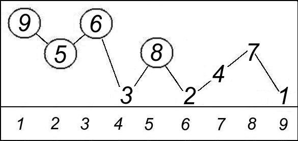
Figure 12: Labelled graph $\mathcal{G}(\sigma_{0})$.

The rest of the algorithm goes from $k=1$ to $n-s=9-4=5$.

• $k=1$ : in Figure 11, the integer $e_{1}(\sigma_{0})=1$ appears in the labels of the dots $v_{p_{1}(\sigma_{0})}(\sigma_{0})=v_{4}(\sigma_{0})$, $v_{p_{2}(\sigma_{0})}(\sigma_{0})=v_{6}(\sigma_{0})$ and $v_{p_{5}(\sigma_{0})}(\sigma_{0})=v_{9}(\sigma_{0})$, so, from

  $$(\sigma_{0}(u_{1}(\sigma_{0})),\sigma_{0}(u_{2}(\sigma_{0})),\sigma_{0}(u_{5}(\sigma_{0}))=(5,3,1),$$

  we label the dot $v_{p_{5}(\sigma_{0})}(\sigma_{0})=v_{9}(\sigma_{0})$ with the integer $e_{1}(\sigma_{0})=1$ and we erase $1$ from any other label, and since the integer $4$ now only appears in the label of the dot $v_{7}(\sigma_{0})$, then we label $v_{7}(\sigma_{0})$ with $4$ (see Figure 11).

• $k=2$: in Figure 11, the integer $e_{2}(\sigma_{0})=2$ appears in the labels of the dots $v_{p_{1}(\sigma_{0})}(\sigma_{0})=v_{4}(\sigma_{0})$ and $v_{p_{2}(\sigma_{0})}(\sigma_{0})=v_{6}(\sigma_{0})$ so, from

  $$(\sigma_{0}(u_{1}(\sigma_{0})),\sigma_{0}(u_{2}(\sigma_{0})))=(5,3),$$

  we label the dot $v_{p_{2}(\sigma_{0})}(\sigma_{0})=v_{6}(\sigma_{0})$ with the integer $e_{2}(\sigma_{0})=2$ and we erase $2$ from any other label, which provides the graph labelled by integers depicted in Figure 12.

• The three steps $k=3,4,5$ change nothing because every dot of $\mathcal{G}(\sigma_{0})$ is already labelled by an integer at the end of the previous step.

So the final version of the labelled graph $\mathcal{G}(\sigma_{0})$ is the one depicted in Figure 12.

3.3 Definition of $\varphi(\sigma)$

By construction of the labelled graph $\mathcal{G}(\sigma)$, the word $y_{1}y_{2}\ldots y_{n}$ (where the integer $y_{i}$ is the label of the vertex $v_{i}(\sigma)$ for all $i$) obviously is a permutation of the set $[n]$, whose planar graph is $\mathcal{G}(\sigma)$.

We define $\varphi(\sigma)\in\mathfrak{S}_{n}$ as this permutation.

For the example $\sigma_{0}=425736981\in\mathfrak{S}_{9}$ whose labelled graph $\mathcal{G}(\sigma_{0})$ is depicted in Figure 12, we obtain $\varphi(\sigma_{0})=956382471\in\mathfrak{S}_{9}$.

In general, by construction of $\tau=\varphi(\sigma)\in\mathfrak{S}_{n}$, we have

$$\tau\left(\text{EXC}(\tau)\right)=\{j_{k}(\sigma),k\in[\text{inv}_{2}(\sigma)]\}$$ (7)

and

$$\text{DES}(\tau)=\begin{cases}\{d^{k}(\sigma),k\in[1,\text{des}_{2}(\sigma)]\}&\text{if $c_{0}(\sigma)=0(\Leftrightarrow d^{0}(\sigma)=0)$},\\ \{d^{k}(\sigma),k\in[0,\text{des}_{2}(\sigma)]\}&\text{otherwise}.\end{cases}$$ (8)

Equality (7) provides

$$\text{exc}(\tau)=\text{inv}_{2}(\sigma).$$

By $d^{k}(\sigma)=d_{2}^{k}(\sigma)+c_{k}(\sigma)$ for all $k$, Equality (8) provides

$$\text{maj}(\tau)=\text{maj}_{2}(\sigma)+\sum_{k\geq 0}c_{k}(\sigma),$$

and by definition of $(c_{k}(\sigma))_{k}$ and Lemma 3.3 we have $\sum_{k\geq 0}c_{k}(\sigma)=\sum_{k\geq 0}c^{0}_{k}(\sigma)=\text{inv}_{2}(\sigma)=\text{exc}(\tau)$ hence

$$\text{maj}(\tau)-\text{exc}(\tau)=\text{maj}_{2}(\sigma).$$

Finally, it is easy to see that $\widetilde{\text{des}_{2}}(\sigma)=\text{des}_{2}(\sigma)$ if and only if $c_{0}(\sigma)=0$, so Equality (8) also provides

$$\text{des}(\tau)=\widetilde{\text{des}_{2}}(\sigma).$$

As a conclusion, we obtain

$$(\text{maj}(\tau)-\text{exc}(\tau),\text{des}(\tau),\text{exc}(\tau))=(\text{maj}_{2}(\sigma),\widetilde{\text{des}_{2}}(\sigma),\text{inv}_{2}(\sigma))$$

as required by Theorem 1.2.

4 Construction of $\varphi^{-1}$

To end the proof of Theorem 1.2, it remains to show that $\varphi:\mathfrak{S}_{n}\rightarrow\mathfrak{S}_{n}$ is surjective. Let $\tau\in\mathfrak{S}_{n}$. We introduce integers $r\geq 0$, $s=\text{exc}(\tau)$, and

$$0\leq d^{0,\tau}<d^{1,\tau}<\ldots<d^{r,\tau}<n$$

such that

$$\text{DES}(\tau) =\{d^{k,\tau},k\in[0,r]\}\cap\mathbb{N}_{>0},$$

$$d^{0,\tau} =0\Leftrightarrow\tau(1)=1.$$

In particular $\text{des}(\tau)=\begin{cases}r&\text{ if $\tau(1)=1$,}\\ r+1&\text{ otherwise}.\end{cases}$

For all $k\in[0,r]$, we define

$$c_{k}^{\tau} =\text{EXC}(\tau)\cap]d^{k-1,\tau},d^{k,\tau}]\text{ (with $d^{-1,\tau}:=0$),}$$

$$d_{2}^{k,\tau} =d^{k,\tau}-c_{k}^{\tau}.$$

We have

$$0=d_{2}^{0,\tau}<d_{2}^{1,\tau}<\ldots<d_{2}^{r,\tau}<n$$

and similarly as Formula 4, we define

$$t_{k}^{\tau}=\min\{d_{2}^{l,\tau},1\leq l\leq k,d_{2}^{l,\tau}=d_{2}^{k,\tau}-(k-l)\}$$ (9)

for all $k\in[r]$.

We intend to construct a graph $\mathcal{H}(\tau)$ which is the linear graph of permutation $\sigma\in\mathfrak{S}_{n}$ such that $\varphi(\sigma)=\tau$.

4.1 Skeleton of the graph $\mathcal{H}(\tau)$

We consider a graph $\mathcal{H}(\tau)$ whose vertices $v_{1}^{\tau},v_{2}^{\tau},\ldots,v_{n}^{\tau}$ (from left to right) are $n$ dots, aligned in a row, among which we box the $d_{2}^{k,\tau}$-th vertex $v_{d_{2}^{k,\tau}}^{\tau}$ for all $k\in[r]$. We also draw the end of an arc of circle above every vertex $v_{j}^{\tau}$ such that $j=\tau(i)$ for some $i\in\text{EXC}(\tau)$.

For the example $\tau_{0}=956382471\in\mathfrak{S}_{9}$ (whose planar graph is depicted in Figure 12), we have $r=\text{des}(\tau_{0})-1=3$ and

$$(c_{k}^{\tau_{0}})_{k\in[0,3]} =(1,2,1,0),$$

$$(d_{2}^{k,\tau_{0}})_{k\in[0,3]} =(1-1,3-2,5-1,8-0)=(0,1,4,8),$$

$$\tau_{0}(\text{EXC}(\tau_{0})) =\{5,6,8,9\},$$

and we obtain the graph $\mathcal{H}(\tau_{0})$ depicted in Figure 13.

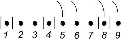
Figure 13: Incomplete graph $\mathcal{H}(\tau_{0})$.

In general, by definition of $\varphi(\sigma)$ for all $\sigma\in\mathfrak{S}_{n}$, if $\varphi(\sigma)=\tau$, then $r=\text{des}_{2}(\sigma)$ and $d_{2}^{k}(\sigma)$ (respectively $c_{k}(\sigma),d^{k}(\sigma),t_{k}(\sigma)$) equals $d_{2}^{k,\tau}$ (resp. $c_{k}^{\tau},d^{k,\tau},t_{k}^{\tau}$) for all $k\in[0,r]$ and $\{j_{l}(\sigma),l\in[\text{inv}_{2}(\sigma)]\}=\tau(\text{EXC}(\tau))$. Consequently, the linear graph of $\sigma$ necessarily have the same skeleton as that of $\mathcal{H}(\tau)$.

The following lemma is easy.

Lemma 4.1.

If $\tau=\varphi(\sigma)$ for some $\sigma\in\mathfrak{S}_{n}$, then :

1. If $j=\tau(l)$ with $l\in\text{EXC}(\tau)$ such that $l\in]d_{2}^{k,\tau},d^{k,\tau}]$, and if $(i,j)\in\text{INV}_{2}(\sigma)$, then $t_{k}^{\tau}\leq i$.

2. A pair $(i,i+1)$ cannot be a $2$-inversion of $\sigma$ if $i\in\text{DES}_{2}(\sigma)$ ($\Leftrightarrow$ if the vertex $v_{i}^{\tau}$ of $\mathcal{H}(\tau)$ is boxed).

3. For all pair $(l,l^{\prime})\in\text{EXC}(\tau)^{2}$, if the labels of the two circles $v_{l}(\sigma)$ and $v_{l^{\prime}}(\sigma)$ can be exchanged without modifying the skeleton of $\mathcal{G}(\sigma)$, let $i$ and $i^{\prime}$ such that $(i,l)\in\text{INV}_{2}(\sigma)$ and $(i^{\prime},l^{\prime})\in\text{INV}_{2}(\sigma)$, then $i<i^{\prime}\Leftrightarrow l<l^{\prime}$.

Consequently, in order to construct the linear graph of a permutation $\sigma\in\mathfrak{S}_{n}$ such that $\tau=\varphi(\sigma)$ from $\mathcal{H}(\tau)$, it is necessary to extend the arcs of circles of $\mathcal{H}(\tau)$ to reflect the three facts of Lemma 4.1. When a vertex is necessarily the beginning of an arc of circle, we draw the beginning of an arc of circle above it. When there is only one vertex $v_{i}^{\tau}$ that can be the beginning of an arc of circle, we complete the latter by making it start from $v_{i}^{\tau}$.

Example 4.2.

For $\tau_{0}=956382471\in\mathfrak{S}_{9}$, the graph $\mathcal{H}(\tau_{0})$ becomes as depicted in Figure 14.

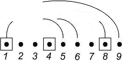
Figure 14: Incomplete graph $\mathcal{H}(\tau_{0})$.

Note that the arc of circle ending at $v_{6}^{\tau_{0}}$ cannot begin at $v_{5}^{\tau_{0}}$ because otherwise, from the third point of Lemma 4.1, and since $(6,8)=(\tau_{0}(l),\tau_{0}(l^{\prime}))$ with $3=l<l^{\prime}=5$, it would force the arc of circle ending at $v_{8}^{\tau_{0}}$ to begin at $v_{i^{\prime}}^{\tau_{0}}$ with $6\leq i^{\prime}$, which is absurd because a permutation $\sigma\in\mathfrak{S}_{9}$ whose linear graph would be of the kind $\mathcal{H}(\tau_{0})$ would have $c_{2}(\sigma)=2\neq 1=c_{2}^{\tau_{0}}$. Also, still in view of the third point of Lemma 4.1, and since $\tau_{0}^{-1}(9)<\tau^{-1}(6)$, the arc of circle ending at $v_{9}^{\tau_{0}}$ must start before the arc of circle ending at $v_{6}^{\tau_{0}}$, hence the configuration of $\mathcal{H}(\tau_{0})$ in Figure 14.

The following two facts are obvious.

Facts 4.3.

If $\tau=\varphi(\sigma)$ for some $\sigma\in\mathfrak{S}_{n}$, then :

1. A vertex $v_{i}^{\tau}$ of $\mathcal{H}(\tau)$ is boxed if and only if $i\in\text{DES}_{2}(\sigma)$. In that case, in particular $i$ is a descent of $\sigma$.

2. If a pair $(i,i+1)$ is not a $2$-descent of $\sigma$ and if $v_{i}^{\tau}$ is not boxed, then $i$ is an ascent of $\sigma$, i.e. $\sigma(i)<\sigma(i+1)$.

To reflect Facts 4.3, we draw an ascending arrow (respectively a descending arrow) between the vertices $v_{i}^{\tau}$ and $v_{i+1}^{\tau}$ of $\mathcal{H}(\tau)$ whenever it is known that $\sigma(i)<\sigma(i+1)$ (resp. $\sigma(i)>\sigma(i+1)$) for all $\sigma\in\mathfrak{S}_{n}$ such that $\varphi(\sigma)=\tau$.

For the example $\tau_{0}=956382471\in\mathfrak{S}_{9}$, the graph $\mathcal{H}(\tau_{0})$ becomes as depicted in Figure 15. Note that it is not known yet if there is an ascending or descending arrow between $v_{7}^{\tau_{0}}$ and $v_{8}^{\tau_{0}}$.

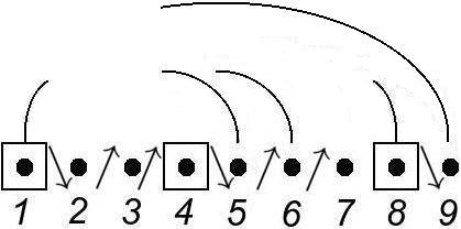
Figure 15: Incomplete graph $\mathcal{H}(\tau_{0})$.

4.2 Completion and labelling of $\mathcal{H}(\tau)$

The following lemma is analogous to the third point of Lemma 4.1 for the dots instead of the circles and follows straightly from the definition of $\varphi(\sigma)$ for all $\sigma\in\mathfrak{S}_{n}$.

Lemma 4.4.

Let $\sigma\in\mathfrak{S}_{n}$ such that $\varphi(\sigma)=\tau$. For all pair $(l,l^{\prime})\in([n]\backslash\text{EXC}(\tau))^{2}$, if the labels of the two dots $v_{l}(\sigma)$ and $v_{l^{\prime}}(\sigma)$ can be exchanged without modifying the skeleton of $\mathcal{G}(\sigma)$, let $k$ and $k^{\prime}$ such that $l=p_{k}(\sigma)$ and $l^{\prime}=p_{k^{\prime}}(\sigma)$, then $\tau(l)<\tau(l^{\prime})\Leftrightarrow\sigma(u_{k}(\sigma))<\sigma(u_{k^{\prime}}(\sigma))$.

Now, the ascending and descending arrows between the vertices of $\mathcal{H}(\tau)$ introduced earlier, and Lemma 4.4, induce a partial order on the set $\{v_{i}^{\tau},i\in[n]\}$:

Definition 4.5.

We define a partial order $\succ$ on $\{v_{i}^{\tau},i\in[n]\}$ by :

• $v_{i}^{\tau}\prec v_{i+1}^{\tau}$ (resp. $v_{i}^{\tau}\succ v_{i+1}^{\tau}$) if there exists an ascending (resp. descending) arrow between $v_{i}^{\tau}$ and $v_{i+1}^{\tau}$;

• $v_{i}^{\tau}\succ v_{j}^{\tau}$ (with $i<j$) if there exists an arc of circle from $v_{i}^{\tau}$ to $v_{j}^{\tau}$;

• if two vertices $v_{i}^{\tau}$ and $v_{j}^{\tau}$ are known to be respectively the $k$-th and $k^{\prime}$-th vertices of $\mathcal{H}(\tau)$ that cannot be the beginning of a complete arc of circle, let $l$ and $l^{\prime}$ be respectively the $k$-th and $k^{\prime}$-th non-exceedance point of $\tau$ (from left to right), if $(l,l^{\prime})$ fits the conditions of Lemma 4.4, then we set $v_{i}^{\tau}\prec v_{j}^{\tau}$ (resp. $v_{i}^{\tau}\succ v_{j}^{\tau}$) if $\tau(l)<\tau(l^{\prime})$ (resp. $\tau(l)>\tau(l^{\prime})$).

Example 4.6.

For the example $\tau_{0}=956382471$, according to the first point of Definition 4.5, the arrows of Figure 15 provide

$$v_{1}^{\tau_{0}}\succ v_{2}^{\tau_{0}}\prec v_{3}^{\tau_{0}}\prec v_{4}^{\tau_{0}}\succ v_{5}^{\tau_{0}}\prec v_{6}^{\tau_{0}}\prec v_{7}^{\tau_{0}}$$

and

$$v_{8}^{\tau_{0}}\succ v_{9}^{\tau_{0}}.$$

Definition 4.7.

A vertex $v_{i}^{\tau}$ of $\mathcal{H}(\tau)$ is said to be minimal on a subset $S\subset[n]$ if $v_{i}^{\tau}\not\succ v_{j}^{\tau}$ for all $j\in S$.

Let

$$1=e_{1}^{\tau}<e_{2}^{\tau}<\ldots<e_{n-s}^{\tau}$$

be the non-exceedance values of $\tau$ (i.e., the labels of the dots of the planar graph of $\tau$).

Algorithm 4.8.

Let $S=[n]$ and $l=1$. While the vertices $\{v_{i}^{\tau},i\in[n]\}$ have not all been labelled with the elements of $[n]$, apply the following algorithm.

1. If there exists a unique minimal vertex $v_{i}^{\tau}$ of $\tau$ on $S$, we label it with $l$, then we set $l:=l+1$ and $S:=S\backslash\{v_{i}^{\tau}\}$. Afterwards,

   1. If $v_{i}^{\tau}$ is the ending of an arc of circle starting from a vertex $v_{j}^{\tau}$, then we label $v^{\tau}_{j}$ with the integer $l$ and we set $l:=l+1$ and $S:=S\backslash\{v_{j}^{\tau}\}$.

   2. If $v^{\tau}_{i}$ is the arrival of an incomplete arc of circle (in particular $i=\tau(l)$ for some $l\in\text{EXC}(\tau)$), we intend to complete the arc by making it start from a vertex $v^{\tau}_{j}$ for some integer $j\in[t_{k}^{\tau},j[$ (where $l\in]d_{2}^{k,\tau},d^{k,\tau}]$) in view of the first point of Lemma 4.1. We choose $v_{j}^{\tau}$ as the rightest minimal vertex on $[t_{k}^{\tau},j[\cap S$ from which it may start in view of the third point of Lemma 4.1, and we label this vertex $v^{\tau}_{j}$ with the integer $l$. Then we set $l:=l+1$ and $S:=S\backslash\{v_{j}^{\tau}\}$.

   Now, if there exists an arc of circle from $v_{j}^{\tau}$ (for some $j$) to $v_{i}^{\tau}$, we apply steps (a),(b) and (c) to the vertex $v_{j}^{\tau}$ in place of $v_{i}^{\tau}$.

2. Otherwise, let $k\geq 0$ be the number of vertices $v_{i}^{\tau}$ that have already been labelled and that are not the beginning of arcs of circles. Let

   $$l_{1}<l_{2}<\ldots<l_{q}$$

   be the integers $l\in[n]$ such that $l\geq\tau(l)\geq e_{k+1}^{\tau}$ and such that we can exchange the labels of dots $\tau(l)$ and $e_{k+1}^{\tau}$ in the planar graph of $\tau$ without modifying the skeleton of the graph. It is easy to see that $q$ is precisely the number of minimal vertices of $\tau$ on $S$. Let $l_{i_{k+1}}=\tau^{-1}(e_{k+1}^{\tau})$ and let $v_{j}^{\tau}$ be the $i_{k+1}$-th minimal vertex (from left to right) on $S$. We label $v_{j}^{\tau}$ with $l$, then we set $l:=l+1$ and $S:=S\backslash\{v_{j}^{\tau}\}$, and we apply steps 1.(a), (b) and (c) to $v_{j}^{\tau}$ instead of $v_{i}^{\tau}$.

By construction, the labelled graph $\mathcal{H}(\tau)$ is the linear graph of a permutation $\sigma\in\mathfrak{S}_{n}$ such that

$$\text{DES}_{2}(\sigma)=\{d_{2}^{k,\tau},k\in[r]\}$$

and

$$\{j_{l}(\sigma),l\in[\text{inv}_{2}(\sigma)]\}=\tau(\text{EXC}(\tau)).$$

Example 4.9.

Consider $\tau_{0}=956382471\in\mathfrak{S}_{9}$ whose unlabelled and incomplete graph $\mathcal{H}(\tau_{0})$ is depicted in Figure 15.

• As stated in Example 4.6, the minimal vertices of $\tau_{0}$ on $S=[9]$ are $(v_{2}^{\tau_{0}},v_{5}^{\tau_{0}},v_{9}^{\tau_{0}})$. Following step 2 of Algorithm 4.8, $k=0$ and the integers $l\in[9]$ such that $\tau_{0}(l)\geq e_{k+1}^{\tau_{0}}=1$ and such that the labels of dots $\tau_{0}(l)$ can be exchanged with $1$ in the planar graph of $\tau_{0}$ (see Figure 12) are $(l_{1},l_{2},l_{3})=(4,6,9)$. By $\tau_{0}^{-1}(1)=9=l_{3}$, we label the third minimal vertex on $[9]$, i.e. the vertex $v_{9}^{\tau_{0}}$, with the integer $l=1$.

  Afterwards, following step 1.(b), since $v_{9}^{\tau_{0}}$ is the arrival of an incomplete arc of circle starting from a vertex $v_{j}^{\tau_{0}}$ with $1=t_{1}^{\tau_{0}}\leq j$, and with $j<5$ because that arc of circle must begin before the arc of circle ending at $v_{6}^{\tau_{0}}$ in view of Fact 3 of Lemma 4.1, we complete that arc of circle by making it start from the unique minimal vertex $v_{j}^{\tau_{0}}$ on $[1,5[$, i.e. $j=2$, and we label $v_{2}^{\tau_{0}}$ with the integer $l=2$ (see Figure 16). Note that as from now we know that the arc of circle ending at $v_{5}^{\tau_{0}}$ necessarily begins at $v_{1}^{\tau_{0}}$, because otherwise $v_{1}^{\tau_{0}}$, being the beginning of an arc of circle, would be the beginning of the arc of circle ending at $v_{6}^{\tau_{0}}$, which is absurd in view of Fact 3 of Lemma 4.1 because $\tau_{0}^{-1}(9)<\tau^{-1}(6)$, so we complete that arc of circle by making it start from $v_{1}^{\tau_{0}}$, which has been depicted in Figure 16.

  

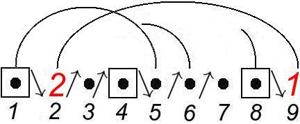
  Figure 16: Beginning of the labelling of $\mathcal{H}(\tau_{0})$.

  We now have $S=[9]\backslash\{2,9\}$ and $l=3$.

• From Figure 16, the minimal vertices on $S=[9]\backslash\{2,9\}$ are $(v_{3}^{\tau_{0}},v_{5}^{\tau_{0}})$. Following step 2 of Algorithm 4.8, $k=1$ and the integers $l\in[9]$ such that $l\geq\tau_{0}(l)\geq e_{k+1}^{\tau_{0}}=2$ and such that the labels of dots $\tau_{0}(l)$ can be exchanged with $2$ in the planar graph of $\tau_{0}$ (see Figure 12) are $(l_{1},l_{2})=(4,6)$. By $\tau_{0}^{-1}(2)=6=l_{2}$, we label the second minimal vertex on $S$, i.e. the vertex $v_{5}^{\tau_{0}}$, with the integer $l=3$.

  Afterwards, following step 1.(a), since $v_{5}^{\tau_{0}}$ is the arrival of the arc of circle starting from the vertex $v_{1}^{\tau_{0}}$, we label $v_{1}^{\tau_{0}}$ with the integer $l=4$ (see Figure 17).

  

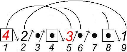
  Figure 17: Beginning of the labelling of $\mathcal{H}(\tau_{0})$.

  We now have $S=[9]\backslash\{1,2,5,9\}$ and $l=5$.

• From Figure 17, the minimal vertices on $S=\{3,4,6,7,8\}$ are $(v_{3}^{\tau_{0}},v_{6}^{\tau_{0}})$. Following step 2 of Algorithm 4.8, $k=2$ and the integers $l\in[9]$ such that $l\geq\tau_{0}(l)\geq e_{k+1}^{\tau_{0}}=3$ and such that the labels of dots $\tau_{0}(l)$ can be exchanged with $3$ in the planar graph of $\tau_{0}$ (see Figure 12) are $(l_{1},l_{2})=(4,7)$. By $\tau_{0}^{-1}(3)=4=l_{1}$, we label the first minimal vertex on $S$, i.e. the vertex $v_{3}^{\tau_{0}}$, with the integer $l=5$ (see Figure 18). Note that as from now we know that the arc of circle ending at $v_{6}^{\tau_{0}}$ necessarily begins at $v_{4}^{\tau_{0}}$ since it it is the only vertex left it may start from. Consequently, the arc of circle ending at $v_{8}^{\tau_{0}}$ necessarily starts from $v_{7}^{\tau_{0}}$ (otherwise it would start from $v_{6}^{\tau_{0}}$, which is prevented by Definition 4.5 because we cannot have $v_{8}^{\tau_{0}}\prec v_{6}^{\tau_{0}}\prec v_{7}^{\tau_{0}}\prec v_{8}^{\tau_{0}}$). The two latter remarks are taken into account in Figure 18.

  

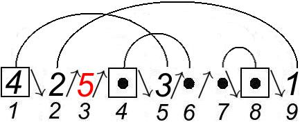
  Figure 18: Beginning of the labelling of $\mathcal{H}(\tau_{0})$.

  We now have $S=\{4,6,7,8\}$ and $l=6$.

• From Figure 18, there is only one minimal vertex on $S=\{4,6,7,8\}$, i.e. the vertex $v_{6}^{\tau_{0}}$. Following step 1 of Algorithm 4.8, we label $v_{6}^{\tau_{0}}$ with $l=6$.

  Afterwards, following step 1.(a), since $v_{6}^{\tau_{0}}$ is the arrival of the arc of circle starting from the vertex $v_{4}^{\tau_{0}}$, we label $v_{4}^{\tau_{0}}$ with the integer $l=7$ (see Figure 19).

  

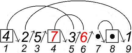
  Figure 19: Beginning of the labelling of $\mathcal{H}(\tau_{0})$.

  We now have $S=\{7,8\}$ and $l=8$.

• From Figure 19, there is only one minimal vertex on $S=\{7,8\}$, i.e. the vertex $v_{6}^{\tau_{0}}$. Following step 1 of Algorithm 4.8, we label $v_{6}^{\tau_{0}}$ with $l=8$.

  Afterwards, following step 1.(a), since $v_{8}^{\tau_{0}}$ is the arrival of the arc of circle starting from the vertex $v_{7}^{\tau_{0}}$, we label $v_{7}^{\tau_{0}}$ with the integer $l=9$ (see Figure 20).

  

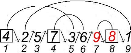
  Figure 20: Labelled graph $\mathcal{H}(\tau_{0})$.

As a conclusion, the graph $\mathcal{H}(\tau_{0})$ is the linear graph of the permutation $\sigma_{0}=425736981\in\mathfrak{S}_{9}$, which is mapped to $\tau_{0}$ by $\varphi$.

Proposition 4.10.

We have $\varphi(\sigma)=\tau$, hence $\varphi$ is bijective.

Proof. By construction , for all $k\in[0,\text{des}_{2}(\sigma)]=[0,r]$,

$$d_{2}^{k}(\sigma) =d^{k,\tau}-c_{k}^{\tau},$$

$$c_{k}(\sigma) =c_{k}^{\tau},$$

$$d^{k}(\sigma) =d_{2}^{k}(\sigma)+c_{k}(\sigma)=d_{2}^{k,\tau}+c_{k}^{\tau}=d^{k,\tau},$$

so $\mathcal{G}(\sigma)$ has the same skeleton as the planar graph of $\tau$, i.e. $\text{DES}(\varphi(\sigma))=\text{DES}(\tau)$ and $\text{EXC}(\varphi(\sigma))=\text{EXC}(\tau)$.

The labels of the circles of $\mathcal{G}(\sigma)$ are the elements of

$$\{j_{l}(\sigma),l\in[s]\}=\tau(\text{EXC}(\tau)),$$

and by construction of $\sigma$, every pair $(l,l^{\prime})\in\text{EXC}(\tau)^{2}$ such that we can exchange the labels $\tau(l)$ and $\tau(l^{\prime})$ in the planar graph of $\tau$ is such that

$$i<i^{\prime}\Leftrightarrow l<l^{\prime}$$

where $(i,\tau(l))$ and $(i,\tau(l^{\prime}))$ are the two corresponding $2$-inversions of $\sigma$. Consequently, by definition of $\varphi(\sigma)$, the labels of the circles of $\mathcal{G}(\sigma)$ appear in the same order as in the planar graph of $\tau$ (i.e. $\varphi(\sigma)(i)=\tau(i)$ for all $i\in\text{EXC}(\varphi(\sigma))=\text{EXC}(\tau)$).

As a consequence, the dots of $\mathcal{G}(\sigma)$ and the planar graph of $\tau$ are labelled by the elements

$$1=e_{1}(\sigma)=e_{1}^{\tau}<e_{2}(\sigma)=e_{2}^{\tau}<\ldots<e_{n-s}(\sigma)=e_{n-s}^{\tau}.$$

As for the labels of the circles, to show that the above integers appear in the same order among the labels of $\mathcal{G}(\sigma)$ and the planar graph of $\tau$, it suffices to prove that

$$\varphi(\sigma)^{-1}(e_{i}^{\tau})<\varphi(\sigma)^{-1}(e_{j}^{\tau})\Leftrightarrow\tau^{-1}(e_{i}^{\tau})<\tau^{-1}(e_{j}^{\tau})$$

for all pair $(i,j)$ such that we can exchange the labels $e_{i}^{\tau}$ and $e_{j}^{\tau}$ in the planar graph of $\tau$ (hence in $\mathcal{G}(\sigma)$ since the two graphs have the same skeleton). This is guaranteed by Definition 4.5 because the vertices $v_{i}^{\tau}$ that are not the beginning of an arc of circle correspond with the labels of the dots of the planar graph of $\tau$.

As a conclusion, the planar graph of $\tau$ is in fact $\mathcal{G}(\sigma)$, i.e. $\tau=\varphi(\sigma)$. ∎

5 Open problem

In view of Formula (2) and Theorem 1.2, it is natural to look for a bijection $\mathfrak{S}_{n}\rightarrow\mathfrak{S}_{n}$ that maps $(\text{maj}_{2},\widetilde{\text{des}_{2}},\text{inv}_{2})$ to $(\text{amaj}_{2},\widetilde{\text{asc}_{2}},\text{ides})$.

Recall that $\text{ides}=\text{des}_{2}$ and that for a permutation $\sigma\in\mathfrak{S}_{n}$, the equality $\widetilde{\text{des}_{2}}(\sigma)=\text{des}_{2}(\sigma)$ is equivalent to $\varphi(\sigma)(1)=1$, which is similar to the equivalence $\widetilde{\text{asc}_{2}}(\tau)=\text{asc}_{2}(\tau)\Leftrightarrow\tau(1)=1$ for all $\tau\in\mathfrak{S}_{n}$.

Note that if $\text{DES}_{2}(\sigma)=\bigsqcup_{p=1}^{r}[i_{p},j_{p}]$ with $j_{p}+1<i_{p+1}$ for all $p$, the permutation $\pi=\rho_{1}\circ\rho_{2}\circ\ldots\circ\rho_{r}\circ\sigma$, where $\rho_{p}$ is the $(j_{p}-i_{p}+2)$-cycle

$$\begin{pmatrix}i_{p}&i_{p}+1&i_{p}+2&\ldots&j_{p}&j_{p}+1\\ \sigma(j_{p}+1)&\sigma(j_{p})&\sigma(j_{p}-1)&\ldots&\sigma(i_{p}+1)&\sigma(i_{p})\end{pmatrix}$$

for all $p$, is such that $\text{DES}_{2}(\sigma)\subset\text{ASC}_{2}(\pi)$ and $\text{INV}_{2}(\sigma)=\text{INV}_{2}(\pi)$. One can try to get rid of the eventual unwanted $2$-ascents $i\in\text{ASC}_{2}(\pi)\backslash\text{DES}_{2}(\sigma)$ by composing $\pi$ with adequate permutations.

References

References

- Eul [55] L. Euler, Institutiones calculi differentialis cum eius usu in analysi finito- rum ac Doctrina serierum, Academiae Imperialis Scientiarum Petropolitanae, St. Petersbourg, 1755.
- HL [12] T. Hance and N. Li, An Eulerian permutation statistic and generalizations, (2012), arXiv:1208.3063.
- LZ [15] Z. Lin and J. Zeng, The -positivity of basic Eulerian polynomials via group actions, (2015), arXiv:1411.3397.
- Mac [15] P. A. MacMahon, Combinatory Analysis, volume 1 and 2, Cambridge Univ. Press, Cambridge, 1915.
- Rio [58] J. Riordan, An Introduction to Combinatorial Analysis, J.Wiley, New York, 1958.
- SW [14] J. Shareshian and M. L. Wachs, Chromatic quasisymmetric functions, (2014), arXiv:1405.4629.