Quantum Statistics of Bosonic Cascades

Abstract

Bosonic cascades formed by lattices of equidistant energy levels sustaining radiative transitions between nearest layers are promising for the generation of coherent terahertz radiation. We show how, also for the light emitted by the condensates in the visible range, they introduce new regimes of emission. Namely, the quantum statistics of bosonic cascades exhibit super-bunching plateaus. This demonstrates further potentialities of bosonic cascade lasers for the engineering of quantum properties of light useful for imaging applications.

Introduction.—Terahertz frequency radiation is a valuable resource for a number of imaging applications in medicine, security screening, and different scientific disciplines tonouchi07a . For this reason a number of solid-state systems have been considered as terahertz sources, where one typically aims to convert an optical frequency photon into a terahertz photon. Even if materials with appropriate transitions can be found, such a procedure is inherently inefficient as the majority of the energy of each optical frequency photon is given up in favour of generating a low-energy terahertz photon. Quantum cascade lasers circumvent this problem, where an optical quantum of energy can be used to generate multiple terahertz photons Kohler2002 ; Liu2013 . While fermionic (electronic) cascades have been realised over 20 years ago Faist1994 , bosonic cascades were only recently designed theoretically based on excitonic transitions in parabolic quantum wells, possibly being placed inside semiconductor microcavities Liew2013 . When using also a THz cavity, bosonic cascades offer the prospects of double stimulation of the emission: by the final exciton state population VCSEL ; Simone and by the terahertz cavity mode population kaliteevski14a ; pervishko .

Stimulated transitions among macroscopically occupied bosonic quantum states are in the heart of bosonic cascade lasers (BCLs), which also act as polariton lasers spontaneously emitting coherent light in the optical frequency range BosonicLasers . Polariton lasers bring the advantage of ultra-low threshold power Christopoulos ; Hoefling ; Bhattachariya and as versatile all-optical platforms sanvitto11a they are expected to constitute building blocks of future optical integrated circuits Circuits , logic elements bistability or polarisation switches switches . The quantum optical properties of polariton lasers have been studied theoretically laussy04a and experimentally richard . The quantum theory of polariton based terahertz sources has been addressed recently delValle2011 . The quantum physics of bosonic cascades is yet to be explored.

In this work, we open a new dimension for BCLs by showing that their emission produces a marked superbunching, thanks to their specificity of making coexist multiple macroscopic coherent states. This makes for a difficult problem to describe quantum mechanically, that we can tackle here with stochastic quantum Langevin equations. This theory of bosonic cascades to describe their statistical properties not only confirms their departures from other mechanisms of lasing paschotta_book08a , it also suggests that they could power imaging applications with resolutions much higher than ever conceived before Gong2015 , thanks to combinations of several assets to go beyond the diffraction limit Hong2012 ; Grujic2013 .

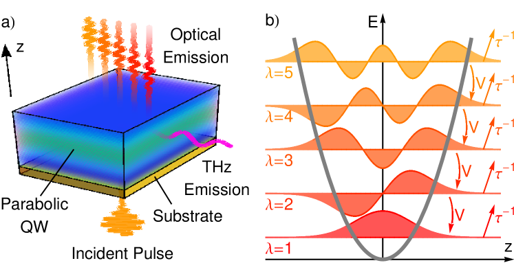
Figure 1: Illustration of a bosonic cascade. a) Structure schematic: a parabolic quantum well is excited with an optical pulse and emits light at a range of frequencies. b) Energy level diagram: the parabolic trapping potential engineers equidistant energy levels and transitions occur between neighbouring levels with transition element $V$. Bosons in each level can decay radiatively, with characteristic decay time $\tau$.

Theory.—We consider a bosonic cascade with $N$ energy levels labelled from $\lambda=1$ to $N$, as illustrated in Fig. 1. The parabolic quantum well makes the levels equidistant in energy Faist . We account for the dominating transitions which are between neighbouring excitonic levels $\lambda+1$ and $\lambda$ and assume for simplicity that all levels decay radiatively with the same rate, $\tau^{-1}$. We assume that the occupation of the terahertz mode fed by the interlevel transitions in the cascade is zero, i.e., there is no terahertz cavity in our model structure. This corresponds to the original version of BCLLiew2013 , where the stimulation of terahertz radiation is achieved due to the macroscopic exciton populations in the bosonic cascade. This simpler configuration already manifests the non-trivial quantum effects of bosonic cascades. The system is thus described by the density matrix $\hat{\rho}$ subject to a quantum Liouville equation:

$$\frac{d\hat{\rho}}{dt}=\frac{1}{2\tau}\sum_{\lambda=1}^{N}\left(\big{[}\hat{a}_{\lambda}^{\vphantom{\dagger}},\hat{\rho}\hat{a}_{\lambda}^{\dagger}\big{]}+\big{[}\hat{a}_{\lambda}^{\vphantom{\dagger}}\hat{\rho},\hat{a}_{\lambda}^{\dagger}\big{]}\right)\\ +\frac{V}{2}\sum_{\lambda=1}^{N-1}\left(\big{[}\hat{a}_{\lambda}^{\dagger}\hat{a}_{\lambda+1}^{\vphantom{\dagger}},\hat{\rho}\hat{a}_{\lambda+1}^{\dagger}\hat{a}_{\lambda}^{\vphantom{\dagger}}\big{]}+\big{[}\hat{a}_{\lambda}^{\dagger}\hat{a}_{\lambda+1}^{\vphantom{\dagger}}\hat{\rho},\hat{a}_{\lambda+1}^{\dagger}\hat{a}_{\lambda}^{\vphantom{\dagger}}\big{]}\right)\,,$$ (1)

where $\hat{a}_{\lambda}$ annihilates a boson from level $\lambda$ and $V$ is the scattering rate Vindependenceonlambda . Dotting this equation with Fock states and neglecting correlations between levels in the Born-Markov approximation leads to the Boltzmann equations, which describe well the average populations of each state and thereby provide the mean-field theory of bosonic cascades Liew2013 . To go beyond this semi-classical description, and in particular to compute the photon statistics, correlations between states must be retained. A brute-force approach, however, is restricted to few levels and each with a modest occupancy. To access the most general cases of bosonic cascades, with macroscopic occupation of the states, we therefore expand the density matrix on the natural basis for this problem, that of coherent states Drummond1980 :

$$\hat{\rho}=\int\mathcal{P}(\alpha_{1},\beta_{1},\ldots,\alpha_{N},\beta_{N})\hat{\Lambda}(\alpha_{1},\beta_{1},\ldots,\alpha_{N},\beta_{N})d\mu\,,$$ (2)

where:

$$\hat{\Lambda}(\alpha_{1},\beta_{1},\ldots,\alpha_{N},\beta_{N})=\frac{|\alpha_{1},\ldots,\alpha_{N}\rangle\langle\beta_{1}^{\ast},\ldots,\beta_{N}^{\ast}|}{\langle\beta_{1}^{\ast},\ldots,\beta_{N}^{\ast}|\alpha_{1},\ldots,\alpha_{N}\rangle}\,,$$ (3)

with $\mathcal{P}$ the positive-P distribution, which differs from the Glauber-Sudarshan distribution in allowing for non-diagonal coherent state projectors. The complex numbers $\alpha_{\lambda}$ and $\beta_{\lambda}$ are independent variables covering the whole complex plane. The integration measure is $d\mu=d^{2}\alpha_{1}d^{2}\beta_{1}\ldots d^{2}\alpha_{N}d^{2}\beta_{N}$ and for ease of notation we write $\vec{\alpha}=(\alpha_{1},\beta_{1},\ldots,\alpha_{N},\beta_{N})$. $\vec{\alpha}_{n}$ will be used to refer to an element of this vector (of length $2N$), while the notations $\alpha_{\lambda}$ and $\beta_{\lambda}$ will still be used where $\lambda$ is the level index. Writing the density matrix in terms of the positive-P distribution (Eq. 2) transforms the master equation Eq. (1) into a Fokker-Planck equation:

$$\frac{\partial\mathcal{P}(\vec{\alpha})}{\partial t}=\frac{1}{2\tau}\sum_{\lambda=1}^{N}\left(\frac{\partial\left(\alpha_{\lambda}\mathcal{P}(\vec{\alpha})\right)}{\partial\alpha_{\lambda}}+\frac{\partial\left(\beta_{\lambda}\mathcal{P}(\vec{\alpha})\right)}{\partial\beta_{\lambda}}\right)\\ +\frac{V}{2}\sum_{\lambda=1}^{N-1}\left\{-\alpha_{\lambda+1}\beta_{\lambda+1}\left(\frac{\partial\left(\alpha_{\lambda}\mathcal{P}(\vec{\alpha})\right)}{\partial\alpha_{\lambda}}+\frac{\partial\left(\beta_{\lambda}\mathcal{P}(\vec{\alpha})\right)}{\partial\beta_{\lambda}}\right)\right.\\ +(\alpha_{\lambda}\beta_{\lambda}+1)\left(\frac{\partial\left(\alpha_{\lambda+1}\mathcal{P}(\vec{\alpha})\right)}{\partial\alpha_{\lambda+1}}+\frac{\partial\left(\beta_{\lambda+1}\mathcal{P}(\vec{\alpha})\right)}{\partial\beta_{\lambda+1}}\right)\\ +2\alpha_{\lambda+1}\beta_{\lambda+1}\frac{\partial^{2}\mathcal{P}(\vec{\alpha})}{\partial\alpha_{\lambda}\partial\beta_{\lambda}}\\ \left.-\frac{\partial^{2}\left(\alpha_{\lambda+1}\alpha_{\lambda}\mathcal{P}(\vec{\alpha})\right)}{\partial\alpha_{\lambda+1}\partial\alpha_{\lambda}}-\frac{\partial^{2}\left(\beta_{\lambda+1}\beta_{\lambda}\mathcal{P}(\vec{\alpha})\right)}{\partial\beta_{\lambda+1}\partial\beta_{\lambda}}\right\}\,.$$ (4)

According to the Ito calculus, a Fokker-Planck equation of the form

$$\frac{\partial\mathcal{P}(\vec{\alpha})}{\partial t}=-\sum_{n}\frac{\partial\left(f_{n}(\vec{\alpha})\mathcal{P}(\vec{\alpha})\right)}{\partial\vec{\alpha}_{n}}+\sum_{nm}\frac{\partial^{2}\left(M_{nm}(\vec{\alpha})\mathcal{P}(\vec{\alpha})\right)}{\partial\vec{\alpha}_{n}\partial\vec{\alpha}_{m}}$$ (5)

with the symmetric matrix $\mathbf{M}(\vec{\alpha})=\textstyle{\frac{1}{2}}\mathbf{B}(\vec{\alpha})\mathbf{B}(\vec{\alpha})^{\mathrm{T}}$ is equivalent to the set of Langevin equations Drummond1980

$$\frac{\partial\vec{\alpha}_{n}}{\partial t}=f_{n}(\vec{\alpha})+B(\vec{\alpha})_{nm}\eta_{m}$$ (6)

where $\eta_{m}$ are independent stochastic Gaussian noise terms, defined by $\langle\eta_{m}(t)\eta_{n}(t^{\prime})\rangle=\delta_{mn}\delta(t-t^{\prime})$. Observable quantities are obtained from averaging the Langevin equation over a stochastically generated ensemble. In particular, the average occupations $\langle\hat{a}_{\lambda}^{\dagger}\hat{a}_{\lambda}^{\vphantom{\dagger}}\rangle=\langle n_{\lambda}\rangle$ and second order correlations $\langle\hat{a}_{\lambda}^{\dagger}\hat{a}_{\lambda}^{\dagger}\hat{a}_{\lambda}^{\vphantom{\dagger}}\hat{a}_{\lambda}^{\vphantom{\dagger}}\rangle$ are given by:

$$\langle\hat{a}_{\lambda}^{\dagger}\hat{a}_{\lambda}^{\vphantom{\dagger}}\rangle =\langle\beta_{\lambda}\alpha_{\lambda}\rangle\,,$$ (7a)

$$\langle\hat{a}_{\lambda}^{\dagger}\hat{a}_{\lambda}^{\dagger}\hat{a}_{\lambda}^{\vphantom{\dagger}}\hat{a}_{\lambda}^{\vphantom{\dagger}}\rangle =\langle\beta_{\lambda}\beta_{\lambda}\alpha_{\lambda}\alpha_{\lambda}\rangle\,.$$ (7b)

The normalized second order correlation function is then defined as $$g_{2,\lambda\lambda}=\langle\hat{a}_{\lambda}^{\dagger}\hat{a}_{\lambda}^{\dagger}\hat{a}_{\lambda}^{\vphantom{\dagger}}\hat{a}_{\lambda}^{\vphantom{\dagger}}\rangle/\langle n_{\lambda}\rangle^{2}$$. By solving Eq. (4) numerically, we are able to study the quantum statistical properties of bosonic cascades under conditions of macroscopic occupations, with several millions of particles.

Two-Level Case.— Considering the simplest case of two levels, we obtain the time dependence of the average populations and second order correlation functions shown in Figs. 2a and b, respectively, for the case where the upper state is initially a coherent state populated with $\langle n_{2}\rangle=5\times 10^{7}$ particles and the ground state is in the vacuum.

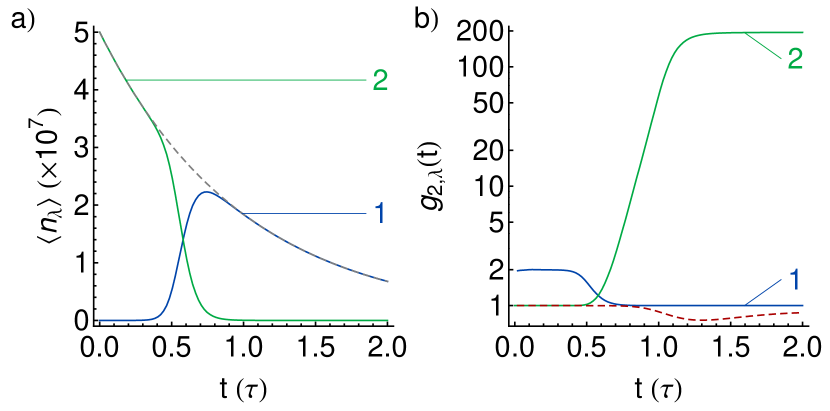
Figure 2: Evolution of two bosonic levels following a coherent pulsed excitation. a) Average level occupations, $\langle n_{\lambda}(t)\rangle$. The dashed curve shows the exponential decay of the total population. b) Second-order correlation function, $g_{2,\lambda}(t)$. The dashed curve shows the cross-correlation function $\langle\hat{a}^{\dagger}_{1}\hat{a}^{\dagger}_{2}\hat{a}_{1}\hat{a}_{2}\rangle/(\langle n_{1}\rangle\langle n_{2}\rangle)$. A coherent state of $\langle n_{2}\rangle=5\times 10^{7}$ particles is assumed in the highest level and we set $V\tau=8.3\times 10^{-7}$ Liew2013 .

The dynamics of relaxation can be well understood: the population from the upper level decreases in time due to radiative emission and transfers to the lower level. At early times, the upper state populates the ground state in a thermal (or chaotic) quantum state, since it merely provides an incoherent input that increases the average population without developing any other independent observable delValle2011 . Consequently, the particle statistics of the lower level is initially $g_{2,\lambda=1}(t)=2$ which is the well known second-order correlation for an incoherent gas of bosons, due to their indistinguishability. Then, as population increases, stimulated emission sets in and the upper state now empties much faster and predominantly into the ground state. This results in the rapid growth of the ground state population until the upper state is so much depleted that it cannot compensate for the ground state’s radiative losses, at which stage the ground state starts to decay through its own radiative channel. In this buildup phase of the ground state, coherence also grows, as seen in the transition from $g_{2,\lambda=1}(t)=2$ to $g_{2,\lambda=1}(t)=1$. Note that the state remains coherent from there on as radiative decay alone does not dephase the condensate. More striking is the statistics of the upper state. While its second-order correlation function was initially unity, as befits a coherent state, and remained essentially unaffected in the first phase of radiative decay and spontaneous emission into the ground state, there is a pronounced super-bunching $g_{2,\lambda=2}(t)\gg 2$ that forms when the state is rapidly emptied. Admirably, just as the statistics of the ground state remains equal to one until complete evaporation, the upper state’s statistics also remains pinned at the value it reached when it completed its transfer. This well defined and high value of $g_{2}$ for a state asymptotically approaching the vacuum is due to the mathematical limit of the two vanishing quantities in Eqs. (7) that exists even for arbitrarily small probabilities of occupation. In practice, numerical simulations are less stable in this region and experimental measurements would also be increasingly difficult. Nevertheless, the most interesting phenomenology is the superbunching that develops in the phase where the upper state quickly empties into the ground state. In this process, where one condensate is sucked by another one, the photons emitted radiatively by the upper state will indeed exhibit a physically observable super-bunched statistics.

The reason for this peculiar behaviour is to be found in the mechanism of coherence buildup. Equation (1) is equivalent to a quantum Boltzmann master equation gardiner97a ; laussy04a , in which formalism coherence—as measured by Glauber’s correlation functions—builds up thanks to population correlations developed by the dynamics, even in the absence of interactions or external potentials. In the conventional case of Bose condensation, the Poisson fluctuations of a single condensed state (usually the ground state), which leads to $g_{n}=1$ for all $n$, are due to this single state adquiring the fluctuations of a macroscopic system laussy12a . Since the central limit theorem states that the distribution of a large number of random variables (the excited states) is a Poisson distribution, so does also fluctuate the condensate in one single state (the ground state). Each excited state taken in isolation contributes very little to the condensate in a macroscopic system and its statistical properties are not significantly altered. In bosonic cascades, however, the asymmetry between ground and excited states is lost since there can be a few macroscopically occupied excited states. This is a peculiar configuration where coherence is adquired from another single coherent state, rather than from a macroscopic ensemble of weakly occupied thermal states (the statistical properties of which do not matter, still following the central limit theorem, as long as they obey generic conditions of independence and normalization). This peculiarity is the reason why the excited state develops such a pronounced superbunching when acting as a reservoir for another condensate to grow in another single state. The fast loss of coherence from a single state to provide for the coherence of another single state, results in the superbunching, or extreme chaos, for the provider that substitutes a macroscopic environment.

Further consequences of this mechanism are that the superbunching should become stronger for bigger initial populations and weaker for more states in the cascade. This is expected from the greater dissimilitude of the bosonic cascade from a single condensate and a macroscopic reservoir: the more levels there are and/or the less they are occupied, the more the system resembles the usual scenario. Indeed, numerical simulations show that this is the case. The dependence of the second order correlation functions, together with the occupation numbers, on the initial occupation number is illustrated in Fig. 3 and confirms the expected behaviour of $g_{2,22}$ with higher populations.

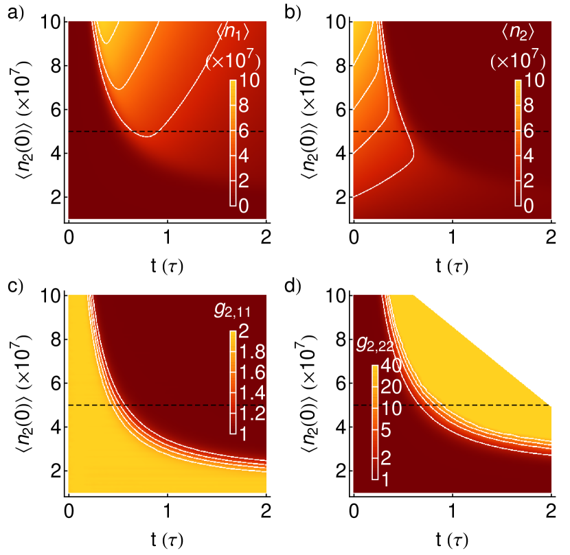
Figure 3: Power dependence of the two-level cascade. a) Average occupation of the lowest level. b) Average occupation of the highest level. c) $g_{2,11}$ of the lowest level. d) $g_{2,22}$ of the highest level. Contours correspond to the values shown in the colour bars. The horizontal dotted line corresponds to the initial occupation considered in Fig. 2. In (d) the value of $g_{2,22}$ is not defined when $\langle n_{2}\rangle$ is small.

The lowest mode maintains the behaviour of being initially thermal, but then becomes a coherent state upon being highly populated, as the upper state makes the transition from coherent to super-bunched light. The greater and sooner the super-bunching, the higher the initial population. The effect of adding more levels in the cascades also results in weaker super-bunching, as expected, but as it also comes with notable features of its own, we will discuss it separately.

Multi-Level Case.— We now consider a larger cascade composed of five levels, still with a macroscopic occupation of the highest excited state ($\langle n_{5}(t=0)\rangle=10^{8}$) and all others empty. The results are shown in Fig. 4.

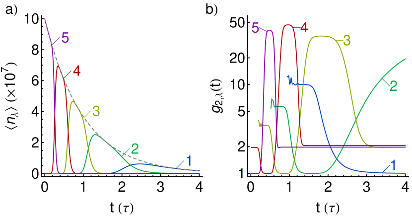
Figure 4: Evolution of five bosonic levels following a coherent pulsed excitation. a) Average level occupations, $\langle n_{\lambda}(t)\rangle$. The dashed curve shows the exponential decay of the total population. b) Second-order correlation function, $g_{2,\lambda}(t)$.

Looking first at the populations (Fig. 4a), we see that there is a staggered oscillation in the successive levels, corresponding to the transfers of particles down through each level of the cascade. The beginning of the relaxation, between the two-highest excited states, is similar to the case already studied, but since the recipient for the highest excited state is also the source for another state below, the dynamics is echoed down the ladder until it reaches the final ground state. In the process, the dynamics slows down and is tamed in intensity, as particles are constantly lost to the environment. The second order correlation functions also exhibit a staggering effect, which can be understood as a generalization of the behaviour observed in Fig. 2 for the two-level case, but with a richer phenomenology. The super-bunching is still observed when the feeding condensate is sucked into the growing one but this process gets disturbed when the latter condensate becomes in its turn the feeding singly-occupied macroscopic state that trades its coherence to the state below it. This releases the drain on the former condensate, which therefore relaxes the super-bunching of what is left of the particles there. In the phase of condensation, the state that grows its coherence does so not only at the expense of its exciting state, but also of the state below. This results in a smaller plateau of super-bunching for the latter state that sandwiches the condensate together with the plateau of large super-bunching from the exciting state. As a result, the particle statistics for each state is an intricate sequence of several plateaus joined by abrupt jumps as the condensate starts to form or starts to empty. For a generic state—that is, one that is not too close from the most excited state or from the ground state—the statistical relief has five plateaus: i) a thermal state starting with, and growing from, the vacuum before the cascade is started; ii) a plateau of “small super-bunching” as it provides coherence from below to its exciting state; iii) a coherent plateau as the state is building its own coherence from the excited state now in its process of avalanche; iv) a plateau of “big superbunching” as the state feeds the state below, becoming super-chaotic in the transfer of coherence; finally, v) a thermal state as the process got transported to states below, with the next state now in its phase of “big superbunching” and that two states below in that of building its coherence. The most relevant plateau is that of stage iv), as it is present for all the excited states and has the stronger signal. All the excited states except that immediately above the ground state ultimately revert to a thermal state, once the peculiar dynamics of bosonic cascade is long gone. The complex concordance of these several stages in statistics with the corresponding ones in populations can be observed in Fig. 4b, showing the beautiful and peculiar dynamics of quantum statistics in bosonic cascades.

Conclusion.— By solving the Fokker-Planck equation for the positive-P representation of a ladder of bosonic states coupled as nearest-neighbors, we could compute the quantum statistics of a bosonic cascade with several levels and for macroscopic occupations. We have shown how the peculiar nature of this system, where coherence is exchanged between single states, results in a super-bunching in the phase where one condensate empties suddenly into the state below. The observation of this strong and striking quantum optical effect could be made in wide parabolic quantum wells where excitons are confined as whole particles. It will not only illustrate fundamental features of coherence buildup in non-interacting bosonic gases, but also provide new venues for imaging applications, in addition to the prospects of implementations in the terahertz bandwidth already offered by these systems.

AK thanks the EPSRC established career fellowship for support. IAS thanks ITN NOTEDEV for support. ASS acknowledges RFBR project 15-02-01060 and FPL the project POLAFLOW. SDL is a Royal Society Research fellow.

References

- (1) M. Tonouchi. Nat. Photon., 1, 97 (2007).
- (2) R. Kohler, A. Tredicucci, F. Beltram, H. E. Beere, E. H. Linfield, A. Giles Davies, D. A. Ritchie, R. C. Lotti, & F. Rossi, Nature, 417, 156 (2002).
- (3) J. Liu, J. Chen, T. Wang, Y. Li, F. Liu, L. Li, L. Wang, & Z. Wang, Solid State Comm., 81, 68 (2013).
- (4) J. Faist, F. Capasso, D. L. Sivco, C. Sirtori, A. L. Hutchinson, & A. Y. Cho, Science, 264, 553 (1994).
- (5) T. C. H. Liew, M. M. Glazov, K. V. Kavokin, I. A. Shelykh, M. A. Kaliteevski, & A. V. Kavokin, Phys. Rev. Lett., 110, 047402 (2013).
- (6) A. V. Kavokin, I. A. Shelykh, T. Taylor, & M. M. Glazov, Phys. Rev. Lett., 108, 197401 (2012).
- (7) S. De Liberato, C. Ciuti, & C. C. Phillips, Phys. Rev. B 87, 241304 (2013).
- (8) M. A. Kaliteevski, K. A. Ivanov, G. Pozina, & A.J. Gallant. Scientific Report, 4, 5444 (2014).
- (9) A. A. Pervishko, T. C. H. Liew, A. V. Kavokin, & I. A. Shelykh, Journal of Physics: Condensed Matter, 26, 085303 (2014).
- (10) A. V. Kavokin, Nature Photon. 7, 591 (2013).
- (11) S. Christopoulos, G. Baldassarri Höger von Högersthal, A. J. D. Grundy, P. G. Lagoudakis, A. V. Kavokin, J. J. Baumberg, G. Christmann, R. Butté, E. Feltin, J.-F. Carlin, & N. Grandjean, Phys. Rev. Lett., 98, 126405 (2007).
- (12) C. Schneider, A. Rahimi-Iman, N. Y. Kim, J. Fischer, I. G. Savenko, M. Amthor, M. Lermer, A. Wolf, L. Worschech, V. D. Kulakovskii, I. A. Shelykh, M. Kamp, S. Reitzenstein, A. Forchel, Y. Yamamoto, & S. Höfling, Nature, 497, 348 (2013).
- (13) P. Bhattacharya, T. Frost, S. Deshpande, M.Z. Baten, A. Hazari, & A. Das, Phys. Rev. Lett. 112, 236802 (2014).
- (14) D. Sanvitto, S. Pigeon, A. Amo, D. Ballarini, M. De Giorgi, I. Carusotto, R. Hivet, F. Pisanello, V. G. Sala, P. S. S. Guimaraes, R. Houdré, E. Giacobino, C. Ciuti, A. Bramati, & G. Gigli, Nat. Photon. 5, 610 (2011).
- (15) T. C. H. Liew, A. V. Kavokin, T. Ostatnicky, M. A. Kaliteevski, I. A. Shelykh, & R. A. Abram, Phys. Rev. B 82, 033302 (2010).
- (16) M. Amthor, T. C. H. Liew, C. Metzger, S. Brodbeck, L. Worschech, M. Kamp, I. A. Shelykh, A. V. Kavokin, C. Schneider, & S. Höfling, Phys. Rev. B 91, 081404(R) (2015).
- (17) A. Amo, T. C. H. Liew, C. Adrados, R. Houdré, E. Giacobino, A. V. Kavokin & A. Bramati, Nature Photon., 4, 361 (2010).
- (18) F. P. Laussy, G. Malpuech, A. Kavokin, & P. Bigenwald, Phys. Rev. Lett., 93, 016402 (2004).
- (19) J. Kasprzak, M. Richard, A. Baas, B. Deveaud, R. André, J.-Ph. Poizat, & Le Si Dang, Phys. Rev. Lett., 100, 067402 (2008).
- (20) E. del Valle & A.V. Kavokin, Phys. Rev. B, 83, 193303 (2011).
- (21) R. Paschotta, Encyclopedia of Laser Physics and Technology, Wiley-VCH (2008).
- (22) W. Gong & S. Han, Sci. Rep., 5, 9280 (2015).
- (23) P. Hong, J. Liu, & G. Zhang, Phys. Rev. A, 86, 013807 (2012).
- (24) T. Grujic, S. R. Clark, D. Jaksch, & D G Angelakis, Phys. Rev. A, 87, 053846 (2013).
- (25) A similar structure has been studied experimentally by M. Geiser et al., Phys. Rev. Lett., 108, 106402 (2012), while in our case there is no need of n-doping: we are interested in transitions between excitonic states confined by the parabolic potential, where excitons are injected by optical pumping.
- (26) Dependencies of on may appear depending on the exact geometry considered Liew2013 , but are not expected to affect the results qualitatively.
- (27) P. D. Drummond & C. W. Gardiner, J. Phys. A: Math. Gen., 13, 2353–2368 (1980).
- (28) C. W. Gardiner & P. Zoller, Phys. Rev. A, 55, 2902 (1997).
- (29) F. P. Laussy in “Exciton-polaritons in microcavities”, Springer Berlin Heidelberg, “Quantum Dynamics of Polariton Condensates”, 172, 1 (2012).