∎

Advanced statistical methods for eye movement analysis and modelling: a gentle introduction

1 Summary

In this Chapter we consider eye movements and, in particular, the resulting sequence of gaze shifts to be the observable outcome of a stochastic process. Crucially, we show that, under such assumption, a wide variety of tools become available for analyses and modelling beyond conventional statistical methods. Such tools encompass random walk analyses and more complex techniques borrowed from the Pattern Recognition and Machine Learning fields.

After a brief, though critical, probabilistic tour of current computational models of eye movements and visual attention, we lay down the basis for gaze shift pattern analysis. To this end, the concepts of Markov Processes, the Wiener process and related random walks within the Gaussian framework of the Central Limit Theorem will be introduced. Then, we will deliberately violate fundamental assumptions of the Central Limit Theorem to elicit a larger perspective, rooted in statistical physics, for analysing and modelling eye movements in terms of anomalous, non-Gaussian, random walks and modern foraging theory.

Eventually, by resorting to Statistical Machine Learning techniques, we discuss how the analyses of movement patterns can develop into the inference of hidden patterns of the mind: inferring the observer’s task, assessing cognitive impairments, classifying expertise.

2 Introduction

Consider Fig. 1: it shows typical scan paths (in this case a succession of saccades and fixations) produced by two human observers on a natural image: circular spots and lines joining spots graphically represent fixations and gaze shifts between subsequent fixations, respectively.

t]

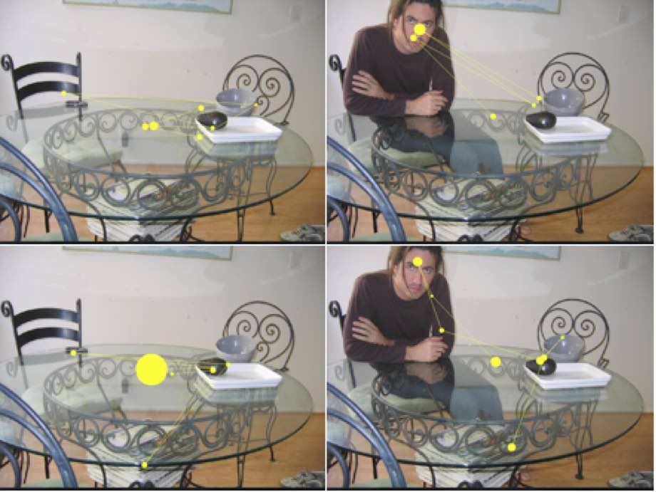
Figure 1: Different scan paths on a pair of images eye-tracked from different human observers. Left, free viewing of a natural scene; right, natural scene embedding a face. The area of yellow disks marking fixations between saccades is proportional to fixation time (images and eye tracking data from the Fixations in FAces dataset

When looking at scan paths, the first question arising is: How can we characterise the shape and the statistical properties of such trajectories? Answering this question entails a data analysis issue. The second question is: What factors determine the shape and the statistical properties? and it relates to the modelling issue.

From a mere research practice standpoint these two issues need not be related (yet, from a more general theoretical standpoint such attitude is at least debatable). A great deal of research can be conducted by performing an eye tracking experiment based on a specific paradigm, and then analysing data by running standard statistical tools (e.g., ANOVA) on scan path “features” such as fixation frequency, mean fixation time, mean saccadic amplitudes, scan path length, etc. The “data-driven” attitude can be preserved even in the case where standard tools are abandoned in favour of more complex techniques borrowed from the Pattern Recognition and Machine Learning fields; for instance, in the endeavour of inferring or classifying the observer’s mental task or the expertise behind his gaze shifts (e.g., henderson2013predicting ; boccignone_jemr2014 ).

In the same vein, it is possible to set up a gaze shift model and successively assess its performance against eye tracking data in terms of classic statistical analyses. For instance, one might set up a probabilistic dynamic model of gaze shifting; then “synthetic” shifts can be generated from the model-based simulation. The distribution of their features can so be compared against the feature distribution of human gaze shifts - on the same stimuli - by exploiting a suitable goodness-of-fit test (e.g., BocFerSMCB2013 , LiberatiASD2017 ).

Clearly, the program of following the data lies at the heart of scientific methodology. When trying to understand a complex process in nature, the empirical evidence is essential. Hypotheses must be compared with the actual data, but the empirical evidence itself may have limitations; that is, it may not be sufficiently large or accurate either to confirm or rule out hypotheses, models, explanations, or assumptions, even when the most sophisticated analytical tools are used.

For eye movement patterns, this issue may be in some cases particularly delicate. Such patterns are, in some sense, a summary of all the motor and perceptual activities in which the observer has been involved during data collection. As sketched in Fig. 2, from a functional standpoint, there are several interacting action / perception loops that drive eye movements. These factors act on different levels of representation and processing: salience, for instance, is a typical bottom-up process, while plans are typical top-down processes schutz2011eye .

b]

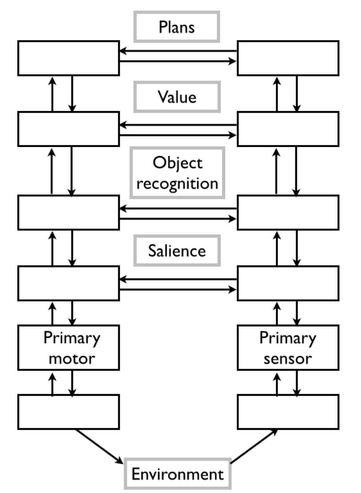
Figure 2: Framework for the control of eye movements. There are several interacting layers of control that influence target selection: the scheme highlights, top to bottom, the contributions of plans, value, object recognition and salience to target selection. The left hand route summarises the motor components, the right hand one, the perceptual components. Figure modified after Schütz et al schutz2011eye

In principle, all such activities should be taken into account when analysing and modelling actual eye movements in visual attention behaviour. Clearly, this is a mind-blowing endeavour.

This raises the question of what is a computational model and how it can support more advanced analyses of experimental data. In this Chapter we discuss a minimal phenomenological model.

At the most general level, the aim of a computational model of visual attention is to answer the question Where to Look Next? by providing:

1. at the computational theory level (in the sense of Marr, Marr ; defining the input/output computation at time $t$), an account of the mapping from visual data of a complex natural scene, say $\mathcal{D}$ (raw image data, or more usefully, features), to a sequence of gaze locations $\mathbf{x}_{F}(1),\mathbf{x}_{F}(2),\cdots$, under a given task $\mathbf{T}$, namely

   $$\mathcal{D}\xmapsto[\mathbf{T}]{}\{\mathbf{x}_{F}(1),\mathbf{x}_{F}(2),\cdots\},$$ (1)

   where the sequence $\{\mathbf{x}_{F}(1),\mathbf{x}_{F}(2),\cdots\}$ can be used to define a scan path (as illustrated in Fig. 3);

2. at the algorithmic level, Marr , a procedure that simulates such mapping (we will not specifically address here the third level of neural realisation Marr ).

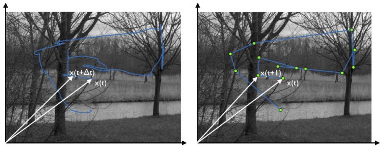
Figure 3: Scan path of an eye-tracked human observer rendered as a temporal sequence of gaze position represented by time-varying location vectors $\mathbf{x}(t)$. The left image shows the continuous raw-data trajectory; the right image, the discretized sequence of fixations and saccades. Images and data are from the Doves dataset van2009doves , which is freely available on the Web

Under this conceptualisation, when considering for instance the input $\mathcal{D}$ in the form of a static scene (a picture), either the raw time series $\{\mathbf{x}_{F}(1),\mathbf{x}_{F}(2),\cdots\}$ or fixation duration and saccade (length and direction) are the only two observable behaviours of the underlying control mechanism. When, $\mathcal{D}$ is a dynamic or time varying scene (e.g. a video), then pursuit needs to be taken also into account. Thus, it is convenient to adopt the generic terms of gaze shifts (either pursuit or saccades) and gaze shift amplitudes. Fixation duration and shift amplitude vary greatly during visual scanning of the scene. As previously discussed, such variation reflects moment-to-moment changes in the visual input, processes occurring at different levels of representation, the state of the oculomotor system and stochastic variability in neuromotor force pulses.

We can summarize this state of affairs by stating that fixation duration and the time series $\{\mathbf{x}_{F}(1),\mathbf{x}_{F}(2),\cdots\}$ (or equivalently, gaze shift lengths and directions) are random variables (RVs) that are generated by an underlying random process. In other terms, the sequence $\{\mathbf{x}_{F}(1),\mathbf{x}_{F}(2),\cdots\}$ is the realisation of a stochastic process, and the goal of a computational theory is to develop a mathematical model that describes statistical properties of eye movements as closely as possible.

Is this minimalist approach to computational modelling of gaze shifts a reasonable one? The answer can be positive if “systematic tendencies” between fixation durations, gaze shift amplitudes and directions of successive eye movements exist and such sequential dependencies can be captured by the stochastic process model. Systematic tendencies in oculomotor behaviour can be thought of as regularities that are common across all instances of, and manipulations to, behavioural tasks. In that case useful information about how the observers will move their eyes can be found.

Indeed, such systematic tendencies or “biases” in the manner in which we explore scenes with our eyes are well known in the literature. One example is provided in Fig. 4 showing the amplitude distribution of saccades and microsaccades that typically exhibit a positively skewed, long-tailed shape.

t]

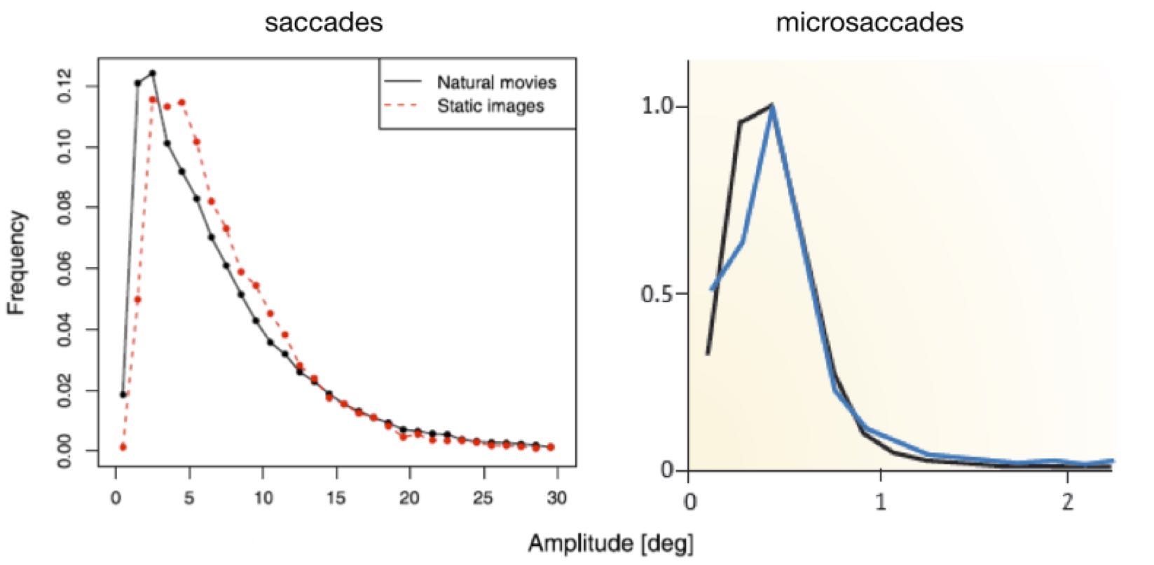
Figure 4: Amplitudes distribution of saccades (on natural movies and static images, left) and microsaccades (right, recordings via video - black - and search coil - blue). In both cases amplitudes follow a positively skewed, long-tailed distribution. Figure modified after Dorr et al dorr2010variability and Martinez-Conde et al martinez2013impact

Other paradigmatic examples of systematic tendencies in scene viewing are tatler2008systematic ; tatler2009prominence : initiating saccades in the horizontal and vertical directions more frequently than in oblique directions; small amplitude saccades tending to be followed by long amplitude ones and vice versa.

Such biases may arise from a number of sources. Tatler and Vincent tatler2009prominence have suggested the following: biomechanical factors, saccade flight time and landing accuracy, uncertainty, distribution of objects of interest in the environment, task parameters.

Understanding biases in how we move the eyes can provide powerful new insights into the decision about where to look in complex scenes. In a remarkable study tatler2009prominence , Tatler and Vincent have shown that a model based solely on these biases and therefore blind to current visual information can outperform salience-based approaches (in particular, they compared against the well known model proposed by Itti et al IttiKoch98 ; walther2006 - see Tom Foulsham’s Chapter in this book for an introduction, and the following Section 4 for a probabilistic framing of saliency models).

Summing up, the adoption of an approach based on stochastic processes bring about significant advantages. First, the analysis and modelling of eye movements can benefit of all the “tools” that have been developed in the field of stochastic processes and time series. For example, the approach opens the possibility of treating visual exploration strategies in terms of random walks, e.g., engbert2006microsaccades ; engbert2011integrated ; carpenter1995neural . Indeed, this kind of conceptual shift happened to the modern developments of econophysics mantegna2000 and finance paul2013stochastic . Further, by following this path, visual exploration can be reframed in terms of foraging strategies an intriguing perspective that has recently gained currency wolfe2013time ; cain2012bayesian ; bfpha04 ; BocFerSMCB2013 ; BocCOGN2014 . Eventually, by embracing the stochastic perspective leads to the possibility of exploiting all the results so far achieved in the “hot” field of Statistical Machine Learning.

Thus, in this Chapter, we pursue the following learning objectives

1. Casting eye movement analysis and modelling in probabilistic terms (Section 4);

2. Understanding the essential concepts of stochastic process, such as Markov processes, and microscopic/macroscopic levels of description (Sections 5, 6);

3. Setting the basics of random walk analyses and modelling of eye movements either within the scope of the Central Limit Theorem or beyond, towards anomalous walks and diffusions (Sections 7);

4. Moving from the analyses of scan path patterns to the inference of mental patterns by introducing the basic tools of modern probabilistic Machine learning (Section 8).

As to the eye movements concepts exploited in the modelling review of Section 4, it is worth referring to the related Chapters of this book.

For all the topics covered hereafter we assume a basic calculus level or at least a familiarity with the concepts of differentiation and integration. Box 1 provides a brief introductory note. However, find an A-level text book with some diagrams if you have not seen this before. Similarly, we surmise reader’s conversance with elementary notions of probability and statistics.

Table 1: Interlude: differential and integral calculus with no pain

Differential calculus deals with the concept of rate of change. The rate of change of a function $f(x)$ is defined as the ratio of the change in $f$ to the change in $x$. Consider Fig.5 showing a plot of $f$ as a function of $x$. There are intervals during which $f$ increases and other intervals where $f$ decreases. We can quantify the ups and downs of the changes in the values of $f$ by estimating the slope, i.e., the change in the variable $f$ over a given interval $\Delta x$, say between $x_{1}$ and $x_{2}$. Denote the interval or average slope by

$$\frac{\Delta f}{\Delta x}=\frac{f(x_{2})-f(x_{2})}{x_{2}-x_{1}}=\frac{f(x+\Delta x)-f(x)}{\Delta x}=\frac{\textsf{rise}}{\textsf{run}},$$

with $\Delta x=x_{2}-x_{1}$. What happens as the interval $\Delta x$ becomes smaller and smaller and approaches zero, formally, $\Delta x\rightarrow 0$?

In that case the interval or average rate of change shrinks to the instantaneous rate of change. This is exactly what is computed by the derivative of $f$ with respect to $x$:

$$\frac{df}{dx}=\lim_{\Delta x\rightarrow 0}\frac{f(x+\Delta x)-f(x)}{\Delta x}.$$

If you prefer thinking in a geometric way, the derivative at a point $x$ provides the slope of the tangent of the curve at $x$.

As an example, we calculate the derivative of the function $f(x)=x^{2}$. First, write the term $f(x+\Delta x)$:

$$f(x+\Delta x)=(x+\Delta x)^{2}=x^{2}+2x\Delta x+\Delta x^{2}$$

Then, subtract $f(x)$ and divide by $\Delta x$:

$$\frac{f(x+\Delta x)-f(x)}{\Delta x}=\frac{x^{2}+2x\Delta x+\Delta x^{2}-x^{2}}{\Delta x}=2x+\Delta x$$

Now in the limit $\Delta x\rightarrow 0$ we shrink $\Delta x$ to zero, i.e.,

$$\lim_{\Delta x\rightarrow 0}2x+\Delta x=2x.$$

Eventually,

$$\frac{d(x^{2})}{dx}=2x.$$

If differential calculus has to do with rates of change, integral calculus deals with sums of many tiny incremental quantities. For instance, consider a continuous function $f$ such as the one plotted in Fig. 6 and the following sum

$$\sum_{i=1}^{n}f(x_{i})\Delta x=f(x_{1})\Delta x+f(x_{2})\Delta x+\cdots+f(x_{n})\Delta x.$$

Here the uppercase greek letter $\sum$ indicates a sum of successive values defined by $i$ and where $\Delta x=\frac{b-a}{n}$ and $x_{i}=a+i\Delta x$. Note that the term

$$f(x_{i})\Delta x=\textsf{height}\times\textsf{width}=\delta A_{i}$$

computes the area $\delta A_{i}$ of the $i$-th rectangle (see Fig. 6). Thus, the (Riemann) sum written above approximates the area defined by the continuous function $f$ within the left and right limits $a$ and $b$, as a the sum of tiny rectangles covering the area under $f$. The sum transforms into the integral

$$\int_{a}^{b}f(x)dx=\lim_{\Delta x\rightarrow 0}\sum_{i=1}f(x_{i})\Delta x$$

when $\Delta x$ shrinks to $0$ (i.e. in the limit $\Delta x\rightarrow 0$) and the number $n$ of intervals grows very large ($n\rightarrow\infty$).

There is a deep connection between integration and differentiation, which is stated by the fundamental theorem of calculus: the processes of integration and differentiation are reciprocal, namely, the derivative of an integral is the original integrand.

t] .

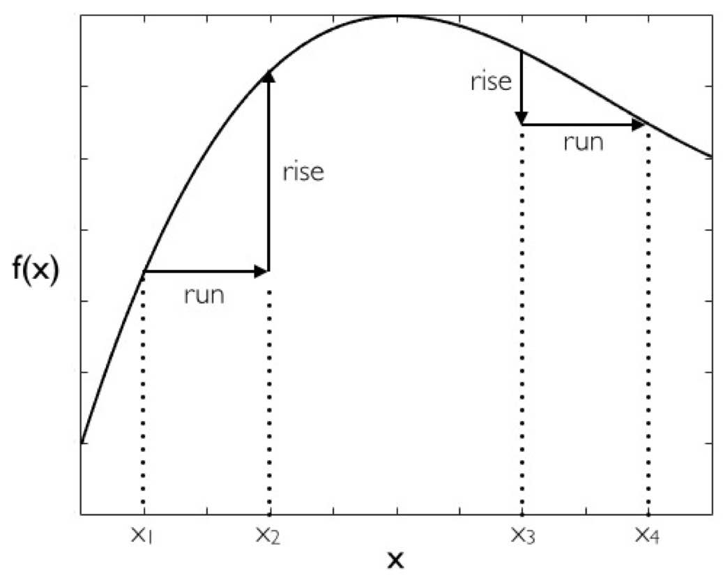
Figure 5: A plot of the values of a function $f$ as a function of $x$, showing a region of negative rate of change or slope (between $x_{1}$ and $x_{2}$) and a region of positive change (between $x_{3}$ and $x_{4}$).

t]

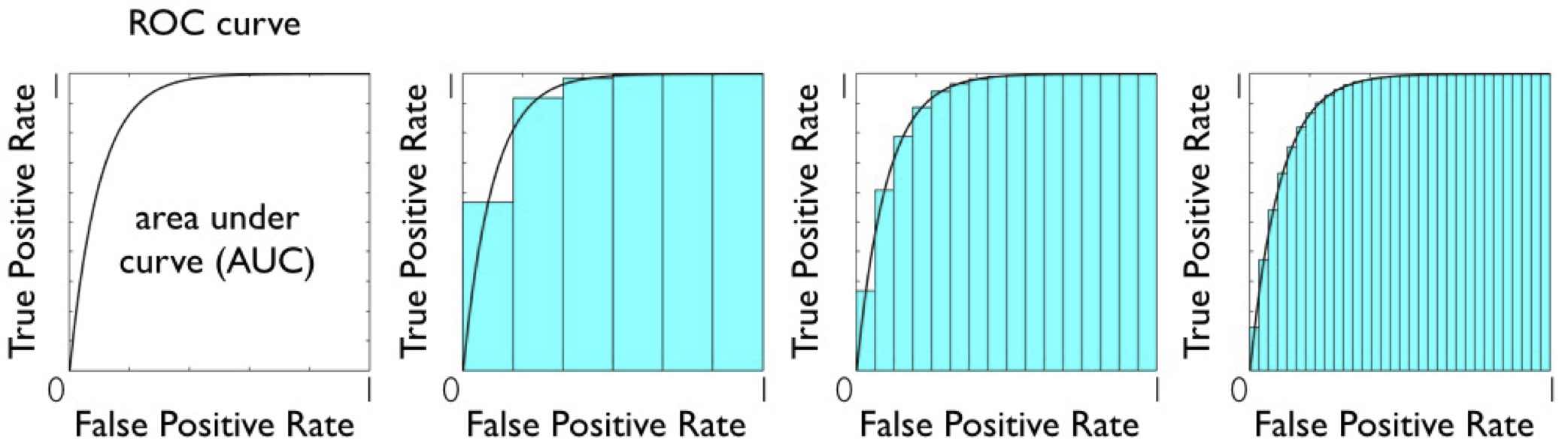
Figure 6: An illustration of the integral concept by using Receiver Operating Characteristic (ROC) analysis, one of the methods to evaluate salience map algorithms. Continuous saliency maps are processed as a binary classifier applied on every pixel: the image pixels of the ground truth, as well as those of the prediction, are classified as fixated (or salient) or as not fixated (not salient). A simple threshold operation is used for this purpose. The ROC curve is exploited to display the classification result for a varying threshold used, each threshold value originating a number of False Positives and True Positives. An ROC curve is shown in the leftmost graph, and it has been obtained by plotting the False Positive Rate (FPR) as a function of the True Positive Rate (TPR). The ROC area, or the area under curve (AUC), provides a measure indicating the overall performance of the classification. The second graph shows the approximate calculus of the AUC as the (Riemann) sum of approximating rectangles as discussed in Box 1. Third and fourth graphs demonstrate how the computed AUC becomes more and more precise for increasing number of rectangles ($n\rightarrow\infty$) and diminishing rectangle widths ($\Delta x\rightarrow 0$). In such limit the sum $\sum$ becomes the integral $\int$.

3 Historical annotations

Stochastic modelling has a long and wide history encompassing different fields. The notion of stochastic trajectories possibly goes back to the scientific poem “De Rerum Natura” (“On the Nature of Things”, circa 58 BC) by Titus Lucretius Carus:

All things keep on in everlasting motion, / Out of the infinite come the particles, / Speeding above, below, in endless dance.

Yet, it is towards the end of the nineteenth century that a major breakthrough occurred. As Gardiner put it gardiner2009stochastic :

Theoretical science up to the end of the nineteenth century can be viewed as the study of solutions of differential equations and the modelling of natural phenomena by deterministic solutions of these differential equations. It was at that time commonly thought that if all initial data could only be collected, one would be able to predict the future with certainty.

Quantum theory, on the one hand, and the concept of chaos (a simple differential equation, due to any error in the initial conditions that is rapidly magnified, can give rise to essentially unpredictable behaviour) on the other, have undermined such a Laplacian conception. However, even without dealing with quantum and chaotic phenomena, there are limits to deterministic predictability. Indeed, the rationale behind this Chapter is that of “limited predictability” gardiner2009stochastic mostly arising when fluctuating phenomena are taken into account. As a matter of fact, stochastic processes are much closer to observations than deterministic descriptions in modern science and everyday life. Indeed, it is the existence of fluctuations that calls out for a statistical account. Statistics had already been used by Maxwell and Boltzmann in their gas theories. But it is Einstein’s explanation einstein1905motion of the nature of Brownian motion (after the Scottish botanist Robert Brown who observed under microscope, in 1827, the random highly erratic motion of small pollen grains suspended in water), which can be regarded as the beginning of stochastic modelling of natural phenomena. Indeed, Einstein’s elegant paper is worth a look, even by the non specialist, since containing all the basic concepts which will make up the subject matter of this Chapter: the Markov assumption, the Chapman-Kolmogorov equation, the random or stochastic differential equation for a particle path, the diffusion equation describing the behaviour of an ensemble of particles, and so forth. Since then, research in the field has quickly progressed. For an historically and technically detailed account the reader might refer to Nelson’s “Dynamical Theories of Brownian Motion”, nelson1967dynamical .

To make a long story short, Einstein’s seminal paper has provided inspiration for subsequent works, in particular that by Langevin langevin1908theorie who, relying upon the analysis of a single particle random trajectory, achieved a different derivation of Einstein’s results. Langevin’s equation was the first example of the stochastic differential equation, namely a differential equation with a random term and whose solution is, in some sense, a random function. Langevin initiated a train of thought that, in 1930, culminated in the work by Ornstein and Uhlenbeck uhlenbeck1930theory , representing a truly dynamical theory of Brownian motion. Although the approach of Langevin was improved and expanded upon by Ornstein and Uhlenbeck, some more fundamental problems remained, markedly related to the differentiability and integrability of a stochastic process. The major contribution to the mathematical theory of Brownian motion has been brought by Wiener wiener1930generalized , who proved that the trajectories of a Brownian process are continuous almost everywhere but are not differentiable anywhere. These problems were addressed by Doob (who came to probability from complex analysis) in his famous paper of 1942 doob1942brownian . Doob aimed at applying the methods and results of modern probability theory to the analysis of the Ornstein-Uhlenbeck distribution. His efforts, together with those of Itô, Markov, Kac, Feller, Bernstein, Lévy, Kolmogorov, Stratonovich and others lead the theory of random processes to become an important branch of mathematics. A nice historical account of stochastic processes from 1950 to the present is provided by Meyer meyer2009stochastic .

Along with theoretical achievements, many more cases of random phenomena materialised in science and engineering. The major developments came in the 1950’s and 1960’s through the analysis of electrical circuits and radio wave propagation. A great deal of highly irregular electrical signals were given the collective name of “noise”: uncontrollable fluctuations in electric circuits (e.g, thermal noise, namely the distribution of voltages and currents in a network due to thermal electron agitation); scattering of electromagnetic waves caused by inhomogeneities in the refractive index of the atmosphere (fading). The fundamental theorem of Nyquist is based on the principle of thermal equilibrium, the same used by Einstein and Langevin papoulis2002probability . Beyond those early days the theory of random processes has become a central topic in the basic training of engineers, and lays the foundation for spectral representation and estimation of signals in noise, filtering and prediction, entropy and information theory papoulis2002probability . Clearly, electrical noise, albeit very important, is far from a unique case. As other examples, one might consider the pressure, temperature and velocity vector of a fluid particle in a turbulent flow. A substantial overlap between the topics of neuroscience and stochastic systems has been acknowledged laing2010stochastic .

Interestingly, beyond the realm of the natural sciences and engineering, analyses of the random character of stock market prices started to gain currency in the 1950’s. Osborne “rediscovered” the Brownian motion of stock markets in 1959 osborne1959brownian . Computer simulations of “microscopic” interacting-agent models of financial markets have been performed as early as 1964 stigler1964public . Brownian motion became an important model for the financial market: Paul Samuelson for his contributions on such topic received the 1970 Nobel Prize in Economics; in 1973, Merton and Scholes, in collaboration with the late Fischer Black, have used the geometric Brownian motion to construct a theory for determining the price of stock options; their achievements were also honoured by the Nobel Prize (Scholes and Merton, 1997). The theory represents a milestone in the development of mathematical finance and today’s daily capital market practice. Interestingly enough, such body of work builds on the early dissertation of a PhD student of Henri Poincaré, named Louis Bachelier. In 1900 Bachelier defended his thesis entitled “Théorie de la Spéculation” at the Sorbonne University of Paris bachelier1900theorie . He had developed, five years before Einstein, the theory of the random walk as a suitable probabilistic description for price fluctuations on the financial market. Unfortunately, such humble application was not acknowledged by the scientific community at that time; hence, Bachelier’s work fell into complete oblivion until the early 1940’s (when Itô used it as a motivation to introduce his calculus). Osborne himself made no mention of it osborne1959brownian . For an historical account of the role played by stochastic processes in the development of mathematical finance theory, see jarrow2004short .

A relevant step, which is of major importance for this Chapter, was taken by Richardson’s work richardson1926atmospheric . Twenty years later Einstein and Langevin works, he presented empirical data related to the “superdiffusion” of an admixture cloud in a turbulent atmosphere being in contradiction with the normal diffusion. Such anomalous diffusion can be explained as a deviation of the real statistics of fluctuations from the Gaussian law. Subsequently, anomalous diffusion in the form of Lévy flights has been discovered in many other physical, chemical, biological, and financial systems (Lévy flights, as we will see, are stochastic processes characterised by the occurrence of extremely long jumps, so that their trajectories are not continuous anymore). The first studies on the subject were those of Kolmogorov kolmogorov1941dissipation on the scale invariance of turbulence in the 1940’s. This topic was later on addressed by many physicists and mathematicians, particularly by Mandelbrot (the father of fractal mathematics). In the 1960s he applied it not only to the phenomenon of turbulence but also to the behaviour of financial markets mandelbrot1963variation . As Mandelbrot lucidly summarised mandelbrot1963variation :

Despite the fundamental importance of Bachelier’s process, which has come to be called “Brownian motion,” it is now obvious that it does not account for the abundant data accumulated since 1900 by empirical economists, simply because the empirical distributions of price changes are usually too “picked” to be relative to samples from Gaussian populations.

An historical but rather technical perspective on anomalous diffusion and Lévy flights is detailed by Dubkov et al. dubkov2008levy ; a more affordable presentation is outlined by Schinckus schinckus2013physicists . Today, these kinds of processes are important to characterise a multitude of systems (e.g., microfluidics, nanoscale devices, genetic circuits that underlie cellular behaviour). Lévy flights are recognised to underlie many aspects of human dynamics and behaviour baronchelli2013levy . Eye movement processes make no exception, as we will see.

Nowadays, the effective application of the theory of random processes and, more generally, of probabilistic models in the real world is gaining pace. The advent of cheap computing power and the developments in Markov chain Monte Carlo simulation produced a revolution within the field of Bayesian statistics around the beginning of the 1990’s. This allowed a true “model liberation”. Computational tools and the latest developments in approximate inference, including both deterministic and stochastic approximations, facilitate coping with complex stochastic process based models that previously we could only dream of dealing with insua2012bayesian . We are witnessing an impressive cross-fertilisation between random process theory and the more recently established areas of Statistical Machine Learning and Pattern Recognition, where the commonalities in models and techniques emerge, with Probabilistic Graphical Models playing an important role in guiding intuition barber2011bayesian .

Table 2: Visual attention models: a brief critical review

In the field of psychology, there exists a wide variety of theories and models on visual attention (see, e.g., the review by Heinke and Humphreys heinke2005computational ). Among the most influential for computational attention systems: the well known Treisman’s Feature Integration Theory (FIT) treisman1980feature ; treisman1998feature ; Wolfe’s Guided Search Model wolfe1994guided , aiming at explaining and predicting the results of visual search experiments; Desimone and Duncan’s Biased Competition Model (BCM, desimone1995neural ), Rensink’s triadic architecture rensink2000dynamic , the Koch and Ullman’s model koch1985shifts , and Tsotsos’ Selective Tuning (ST) model tsotsos1995modelling.

Other psychophysical models have addressed attention modelling in a more formal framework. One notable example is Bundensen’s Theory of Visual Attention (TVA, bundesen1998 ), further developed by Logan into the CODE theory of visual attention (CTVA, logan1996code ). Also, theoretical approaches to visual search have been devised by exploiting Signal Detection Theory palmer2000psychophysics .

At a different level of explanation, other proposals have been conceived in terms of connectionist models, such as MORSEL (Multiple Object Recognition and attentional SELection, mozer1987 ), SLAM (SeLective Attention Model) phaf1990slam , SERR (SEarch via Recursive Rejection) humphreys1993search , and SAIM (Selective Attention for Identification Model by Heinke and Humphreys heinke2003attention ) subsequently refined in the Visual Search SAIM (VS-SAIM) heinke2011modelling .

To a large extent, the psychological literature was conceived and fed on simple stimuli, nevertheless the key role that the above models continue to play in understanding attentive behaviour should not be overlooked. For example, many current computational approaches, by and large, build upon the bottom-up salience based model by Itti et al. IttiKoch98 , which in turn is the computational counterpart of Koch and Ullman and Treisman’s FIT models. The seminal work of Torralba et al. Torralba , draws on an important component of Rensink’s triadic architecture rensink2000dynamic , in that it considers contextual information such as gist - the abstract meaning of a scene, e.g., a city scene, etc. - and layout - the spatial arrangement of the objects in a scene. More recently, Wischnewski et al. anna have presented a computational model that integrates Bundensen’s TVA bundesen1998 .

However, in the last three decades, psychological models have been adapted and extended in many respects, within the computational vision field where the goal is to deal with attention models and systems that are able to cope with natural complex scenes rather than simple stimuli and synthetical images (e.g., see frintrop2010 and the most recent review by Borji and Itti BorItti2012 ). The adoption of complex stimuli has sustained a new brand of computational theories, though this theoretical development is still at an early stage: up to this date, nobody has really succeeded in predicting the sequence of fixations of a human observer looking at an arbitrary scene frintrop2010 . This is not surprising given the complexity of the problem. One might think that issues of generalisation from simple to complex contexts are nothing more than a minor theoretical inconvenience; but, indeed, the generalisation from simple to complex patterns might not be straightforward. As it has been noted in the case of attentive search, a model that exploits handpicked features may fail utterly when dealing with realistic objects or scenes zelinsky2008theory .

Current approaches within this field suffer from a number of limitations: they mostly rely on a low-level salience based representation of the visual input, they seldom take into account the task’s role, and eventually they overlook the eye guidance problem, in particular the actual generation of gaze-shifts (but see Tatler et al TatlerBallard2011eye for a lucid critical review of current methods). We will discuss such limitations in some detail in Section 4.

4 A probabilistic tour of current computational models of eye movements and visual attention (with some criticism)

Many models in psychology and in the computational vision literature have investigated limited aspects of the problem of eye movements in visual attention behaviour (see Box 2, for a quick review). And, up to now, no model has really succeeded in predicting the sequence of fixations of a human observer looking at an arbitrary scene frintrop2010 .

Table 3: Dangerous relationships: A rendezvous with Bayesian Probabilities

We assume the readers to be already familiar with the elementary notions (say, undergrad level) of probability and random variables (RVs). Thus, a warning. Sometimes we talk about probabilities of events that are “out there” in the world. The face of a flipped coin is one such event. But sometimes we talk about probabilities of events that are just possible beliefs “inside the head.” Our belief about the fairness of a coin is an example of such an event. Clearly, it might be bizarre to say that we randomly sample from our beliefs, like we sample from a sack of coins. To cope with such embarrassing situation, we shall use probabilities to express our information and beliefs about unknown quantities. $P(A)$ denotes the probability that the event $A$ is true. But event $A$ could stand for logical expressions such as “there is a red car in the bottom of the scene” or “an elephant will enter the pub”. In this perspective, probability is used to quantify our uncertainty about something; hence, it is fundamentally related to information rather than repeated trials. Stated more clearly: we are adopting the Bayesian interpretation of probability in this Chapter.

Fortunately, the basic rules of probability theory are the same, no matter which interpretation is adopted (but not that smooth, if we truly addressed inferential statistics). For what follows, we just need to refresh a few.

Let $X$ and $Y$ be RVs, that is numbers associate to events. For example, the quantitative outcome of a survey, experiment or study is a RV; the amplitudes of saccades or the fixation duration times recorded in a trial are RVs. In Bayesian inference a RV (either discrete or continuous) is defined as an unknown numerical quantity about which we make probability statements. Call $P(X,Y)$ their joint probability. The conditional probability of $X$ given $Y$ is:

$$P(X\mid Y)\equiv\frac{P(X,Y)}{P(Y)}\text{ if }P(Y)\neq 0.$$ (2)

In Bayesian probability we always deal with conditional probabilities: at least we condition on the assumptions or set of hypotheses $\mathcal{H}$ on which the probabilities are based. In data modelling and Machine Learning, the following holds Mackay :

You cannot do inference without making assumptions

Then, the rules below will be useful:

Product rule (or chain rule)

$$P(X,Y\mid\mathcal{H})=P(X\mid Y,\mathcal{H})P(Y\mid\mathcal{H})$$ (3)

Sum rule (marginalisation)

$$P(Y\mid\mathcal{H}) = \sum_{X}P(X,Y\mid\mathcal{H})\text{ (discrete RVs)}$$ (4)

$$P(Y\mid\mathcal{H}) = \int_{X}P(X,Y\mid\mathcal{H})dX\text{ (continuous RVs)}$$ (5)

Bayes’ rule (see Fig. 7 for a simple example)

$$P(X\mid Y,\mathcal{H})=\frac{P(Y\mid X,\mathcal{H})P(X\mid\mathcal{H})}{P(Y\mid\mathcal{H})}\leftrightarrow\text{ posterior}=\frac{\text{ likelihood}\times\text{prior}}{\text{evidence}}$$ (6)

To avoid burying the reader under notations, we have used $P(\cdot)$ to denote both the probability of a discrete outcome (probability mass function, PMF) and the probability of a continuous outcome (probability density function, pdf). We let context make things clear. Also, we may adopt the form $X=x$ for a specific choice of value (or outcome) of the RV $X$. Briefer notation will sometimes be used: for example, $P(X=x)$ may be written as $P(x)$. A bold $\mathbf{X}$ might denote a set of RVs or a random vector/matrix.

The “bible” of the Bayesian approach is the treatise of Jaynes jaynes2003probability . A succinct introduction with an eye to inference and learning problems can be found in Chapter 2 of the beautiful book by MacKay Mackay , which is also available for free online, http://www.inference.phy.cam.ac.uk/mackay/itila/.

t] .

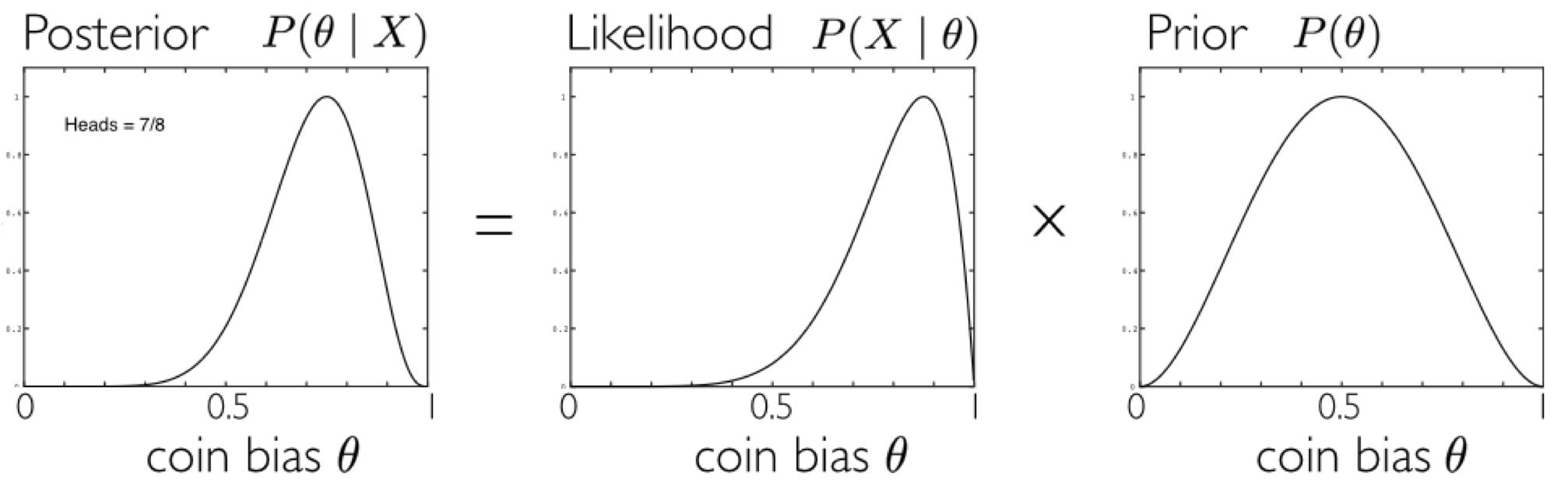
Figure 7: An illustration of the use of the Bayes’ rule for inferring the bias of a coin on the basis of coin tossing results. The prior probability $P(\theta)$ for the coin bias $\theta$ captures the assumption that the coin is likely to be a fair one (the pdf is “peaked” on $\theta=0.5$). However, $7$ heads occur after $8$ tosses. Such experimental result is captured by the shape of the likelihood $P(X\mid\theta)$ strongly biased to the right. Bayes’ rule computes the posterior pdf $P(\theta\mid X)$ by “updating” the initial prior through the “observed” likelihood (the evidence term is not shown in the figure and it has been treated as a normalisation factor to constrain probabilities between $0$ and $1$)

The issue of devising a computational model of eye guidance as related to visual attention - i.e. answering the question Where to Look Next? in a formal way - can be set in a probabilistic Bayesian framework (see Box 3 for a brief introduction). Tatler and Vincent tatler2009prominence have re-phrased this question in terms of Bayes’ rule:

$$\overbrace{P(\mathbf{x}\mid\mathcal{D})}^{\text{posterior prob. of gaze shift }}=\frac{\overbrace{P(\mathcal{D}\mid\mathbf{x})}^{\text{data likelihood under the shift}}}{P(\mathcal{D})}\overbrace{P(\mathbf{x})}^{\text{gaze shift prior}},$$ (7)

where $\mathbf{x}=\mathbf{x}_{F}(t)-\mathbf{x}_{F}(t-1)$ is the random vector representing the gaze shift (in tatler2009prominence , saccades), and $\mathcal{D}$ generically stands for the input data. As Tatler and Vincent put it, “The beauty of this approach is that the data could come from a variety of data sources such as simple feature cues, derivations such as Itti’s definition of salience, object-or other high-level sources”.

In Eq. 7, the first term on the right hand side accounts for the likelihood of particular visual data (e.g., features, such as edges or colors) occurring at a gaze shift target location normalized by $P(\mathcal{D})$ the pdf of these visual data occurring in the environment. As we will see in brief, this first term bears a close resemblance to approaches previously employed to evaluate the possible involvement of visual features in eye guidance.

Most interesting, and related to issues raised in the introductory Section, is the Bayesian prior $P(\mathbf{x})$, i.e., the probability of shifting the gaze to a location irrespective of the visual information at that location. Indeed, this term will encapsulate any systematic tendencies in the manner in which we explore scenes with our eyes. The striking result obtained by Tatler and Vincent tatler2009prominence is that if we learn $P(\mathbf{x})$ from actual observer’s behaviour, then we can sample gaze shifts (cfr. Box 4), i.e.,

$$\mathbf{x}(t)\sim P(\mathbf{x}),\;\;\;\;t=1,2,\cdots$$ (8)

so to obtain scan paths that, blind to visual information, out-perform feature-based accounts of eye guidance tatler2009prominence : $0.648$ area under the receiver operator curve (AUC, which has been illustrated in Fig. 6) as opposed to $0.593$ for edge information (namely, an orientation map computed from edge maps constructed over a range of spatial scales, by convolving the image with four oriented odd-phase Gabor filters) and $0.565$ for salience information as derived through the Itti et al model  IttiKoch98

Table 4: When God plays dice: the art (and magic) of sampling

Eye movements can be considered a natural form of sampling. Another example of actual physical sampling is tossing a coin, as in the example illustrated in Fig. 8, or throwing dice. Nevertheless, we can (and need to) simulate sampling that occurs in nature (and thus the underlying process). Indeed, for both computational modelling and analysis we assume of being capable of the fundamental operation of generating a sample $\mathbf{X}=\mathbf{x}$ from a probability distribution $P(\mathbf{X})$. We denote the sampling action via the $\sim$ symbol:

$$\mathbf{x}\sim P(\mathbf{X}).$$ (9)

For instance, tossing a coin like we did in the example of Fig. 7 can be simulated by sampling $\mathbf{x}$ from a Bernoulli distribution, $\mathbf{x}\sim Bern(\mathbf{X};\theta)$, where $\theta$ is the parameter standing for the coin bias ($\theta=\frac{1}{2}=0.5$ denotes a fair coin).

Surprisingly, to simulate nature, we need a minimal capability: that of generating realisations of RVs uniformly distributed on the interval $\left[0,1\right]$. In practical terms, we just need a programming language or a toolbox in which a rand() function is available implementing the $\mathbf{u}\sim Uniform(0,1)$ operation. Indeed, given the RVs $\mathbf{u}$, we can generate the realisations of any other RV with appropriate “transformations” of $\mathbf{u}$.

There is a wide variety of “transformations” for generating samples, from simple ones (e.g. inverse transform sampling and rejection sampling) to more sophisticated, like those relying on Markov Chain Monte Carlo methods (e.g., Gibbs sampling and Metropolis sampling). Again, MacKay’s book Mackay provides a very clear introduction to the art of random sampling.

You can qualitatively assess the results of your computational sampling procedure using sample histograms. Recall from your basic statistic courses that an histogram is an empirical estimate of the probability distribution of a continuous variable. It is obtained by ”binning” the range of values – that is, by dividing the entire range of values into a series of small intervals –, and then counting how many values fall into each interval. Intuitively, if we look at the empirical distribution of the set of samples $\{\mathbf{x}(t)\}_{t=1}^{T}$ obtained for a large number $T$ of sampling trials $\mathbf{x}(t)\sim P(\mathbf{X})$, $t=1,2,\cdots,T$, we expect the shape of the histogram to approximate the originating theoretical density. Examples are provided in Fig. 8 where $1000$ samples have been generated experimenting with the Uniform distribution, the Gaussian distribution and the Cauchy distribution, respectively.

t] .

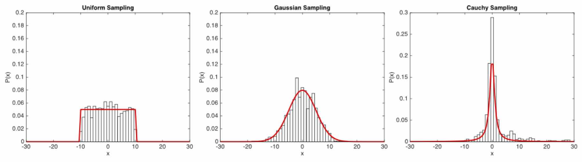
Figure 8: From left to right, the empirical distributions (histograms) for $n=1000$ samples drawn from Uniform, Gaussian and and Cauchy pdfs. Uniform and Gaussian sampling have been performed via the Matlab functions rand() and randn(), respectively; samples from the Cauchy pdf have been generated resorting to Metropolis sampling. Each histogram is overlaid with the generating theoretical density depicted as a continuous red curve

Learning is basically obtained by empirically collecting through eye tracking the observer’s behaviour on an image data set (formally, the joint pdf $P(\mathbf{x},\mathcal{D}$) and then factoring out the informative content of the specific images, briefly, via marginalisation,i.e., $P(\mathbf{x})=\sum_{\mathcal{D}}P(\mathbf{x},\mathcal{D})$.

Note that the apparent simplicity of the prior term $P(\mathbf{x})$ hides a number of subtleties. For instance, Tatler and Vincent expand the random vector $\mathbf{x}$ in terms of its components, amplitude $l$ and direction $\theta$. Thus, $P(\mathbf{x})=P(l,\theta)$. This simple statement paves the way to different options. First easy option: such RVs are marginally independent, thus, $P(l,\theta)=P(l)P(\theta)$. In this case, gaze guidance, solely relying on biases, could be simulated by expanding Eq. (8) via independent sampling of both components, i.e. at each time $t$, $l(t)\sim P(l(t)),\theta(t)\sim P(\theta(t))$. Alternative option: conjecture some kind of dependency, e.g. amplitude on direction, so that $P(l,\theta)=P(l\mid\theta)P(\theta)$. In this case, the gaze shift sampling procedure would turn into the sequence $\widehat{\theta}(t)\sim P(\theta(t)),l(t)\sim P(l(t)\mid\widehat{\theta}(t))$. Further: assume that there is some persistence in the direction of the shift. This gives rise to a stochastic process in which subsequent directions are correlated, i.e., $\theta(t)\sim P(\theta(t)\mid\theta(t-1))$, and so on.

t]

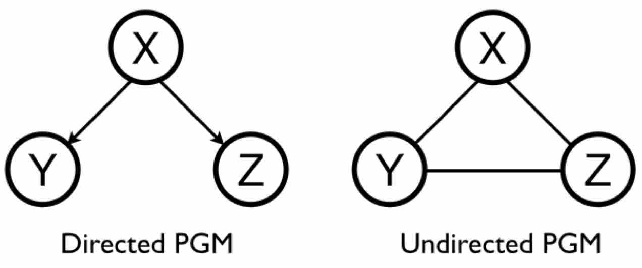
Figure 9: Probabilistic Graphical Models: a directed PGM (left, a.k.a. Bayesian Network) and an undirected PGM (right, a.k.a. Markov Random Field). Nodes represents RVs and arcs express probabilistic relationships between RVs

Table 5: Probabilistic Graphical Models (PGM)

A PGM koller2009probabilistic is a graph-based representation (see Fig. 9) where nodes (also called vertices) are connected by arcs (or edges). In a PGM, each node represents a RV (or group of RVs), and the arcs express probabilistic relationships between these variables. Graphs where arcs are arrows are directed PGM, a generalisation of Bayesian Networks (BN), well known in the Artificial Intelligence community. The other major class of PGMs are undirected PGM (Fig. 9, right), in which the links have no directional significance, but are suitable to express soft constraints between RVs. The latter are also known as Markov Random Fields (MRF), largely exploited in Computer Vision.

We shall focus on directed PGM representations where arrows represent conditional dependencies (Fig. 9, left). For instance the arrow $X\rightarrow Y$ encodes the probabilistic dependency of RV $Y$ on $X$ quantified through the conditional probability $P(Y\mid X)$. Note that arrows do not generally represent causal relations, though in some circumstances it could be the case. We will mainly exploit PGMs as a descriptive tool: indeed, 1) they provide a simple way to visualise the structure of a probabilistic model and can be used to design and motivate new models; 2) they offer insights into the properties of the model, including conditional independence properties, which can be obtained by inspection of the graph.

PGMs capture the way in which the joint distribution over all of the RVs can be decomposed into a product of factors each depending only on a subset of the variables. Assume that we want to describe a simple object-based attention model (namely, the one presented at the centre of Figure 10), so to deal with: (i) objects (e.g., red triangles vs. blue squares), (ii) their possible locations, and (iii) the visual features sensed from the observed scene. Such “world’ can be described by the joint pdf $P(Objects,Location,Features)$ which we denote, more formally, through the RVs $O,L,F$: $P(Objects,Location,Features)\equiv P(O,L,F)$. Recall that - via the product rule - the joint pdf could be factorised in a combinatorial variety of ways, all equivalent and admissible:

$$P(O,L,F) = P(O\mid L,F)P(L\mid F)P(F)$$

$$= P(L\mid O,F)P(O\mid F)P(F)$$

$$= P(F\mid O,L)P(O\mid L)P(L)$$

$$= \cdots$$

The third factorisation is, actually, the meaningful one: the likelihood of observing certain features (e.g, color) in the visual scene depends on what kind of objects are present and on where they are located; thus, the factor $P(F\mid O,L)$ makes sense. $P(L)$ represents the prior probability of choosing certain locations within the scene (e.g., it could code the center bias effect tatler2007central ). Eventually, the $P(O\mid L)$ factor might code the prior probability of certain kinds of objects (e.g., we may live in a world where red triangles are more frequent than blue squares). As to $P(O\mid L)$ we can assume that the object location and object identity are independent, formally, $P(O\mid L)=P(O)$, finally leading to

$$P(O,L,F)=P(F\mid O,L)P(O)P(L).$$ (11)

This factorisation is exactly that captured by the structure of the directed PGM presented at the centre of Figure 10. Indeed, the graph renders the most suitable factorisation of the unconstrained joint pdf, under the assumptions and the constraints we are adopting to build our model. We can “query” the PGM for making any kind of probabilistic inference. For instance, we could ask what is the posterior probability $P(O,L\mid F)$ of observing certain objects at certain locations given the observed features. By using the definition of conditional probability and Eq. 11:

$$P(O,L\mid F)=\frac{P(O,L,F)}{P(F)}=\frac{P(F\mid O,L)P(O)P(L)}{P(F)}$$ (12)

Complex computations for inference and learning in sophisticated probabilistic models can be expressed in terms of graph-based algorithms. PGMs are a formidable tool to such end, and nowadays are widely adopted in modern probabilistic Machine Learning and Pattern Recognition. An affordable introduction can be found in Bishop BishopPRML . The PGM “bible” is the textbook by Koeller koller2009probabilistic .

To summarise, by simply taking into account the prior $P(\mathbf{x})$, a richness of possible behaviours and analyses are brought into the game. To further explore this perspective, we recommend the thorough and up-to-date review by Le Meur and Coutrot le2016introducing .

Unfortunately, most computational accounts of eye movements and visual attention have overlooked this issue. We noticed before, by inspecting Eq. (7) that the term $\frac{P(\mathcal{D}\mid\mathbf{x})}{P(\mathcal{D})}$ bears a close resemblance to many approaches proposed in the literature. This is an optimistic view. Most of the approaches actually discard the dynamics of gaze shifts, say $\mathbf{x}_{F}(t)\rightarrow\mathbf{x}_{F}(t+1)$, implicitly captured through the shift vector $\mathbf{x}(t)$. In practice, most models are more likely to be described by a simplified version of Eq. (7):

$$\overbrace{P(\mathbf{x}_{F}\mid\mathcal{D})}^{\text{posterior prob. of gazing at}}=\frac{\overbrace{P(\mathcal{D}\mid\mathbf{x}_{F})}^{\text{data likelihood under gaze at}}}{P(\mathcal{D})}\overbrace{P(\mathbf{x}_{F})}^{\text{prior prob. of gazing at}},$$ (13)

By careful inspection, it can be noted that the posterior $P(\mathbf{x}_{F}\mid\mathcal{D})$ answers the query “What is the probability of fixating location $\mathbf{x}_{F}$ given visual data $\mathcal{D}$?”. Further, the prior $P(\mathbf{x}_{F})$ accounts for the probability of fixating location $\mathbf{x}_{F}$ irrespective of the visual information at that location. The difference between Eq. 7 and Eq. 13 is subtle. But, as a matter of fact, Eq. 13 bears no dynamics. In probabilistic terms we may re-phrase this result as the outcome of an assumption of independence:

$$P(\mathbf{x})=P(\mathbf{x}_{F}(t)-\mathbf{x}_{F}(t-1))\simeq P(\mathbf{x}_{F}(t)\mid\mathbf{x}_{F}(t-1))=P(\mathbf{x}_{F}(t)).$$

To make things even clearer, let us explicitly substitute $\mathbf{x}_{F}$ with a RV $\mathbf{L}$ denoting locations in the scene, and $\mathcal{D}$ with RV $\mathbf{F}$ denoting features (whatever they may be); then Eq. 13 boils down to the following

$$\overbrace{P(\mathbf{L}\mid\mathbf{F})}^{\text{posterior prob. of selecting location L}}=\frac{\overbrace{P(\mathbf{F}\mid\mathbf{L})}^{\text{feature likelihood under location L}}}{P(\mathbf{F})}\overbrace{P(\mathbf{L})}^{\text{prior prob. of location L}}$$ (14)

The feature-based Probabilistic Graphical Model underlying this query (see Box 5 for a brief PGM overview) is a very simple one and is represented on the left of Fig. 10.

t]

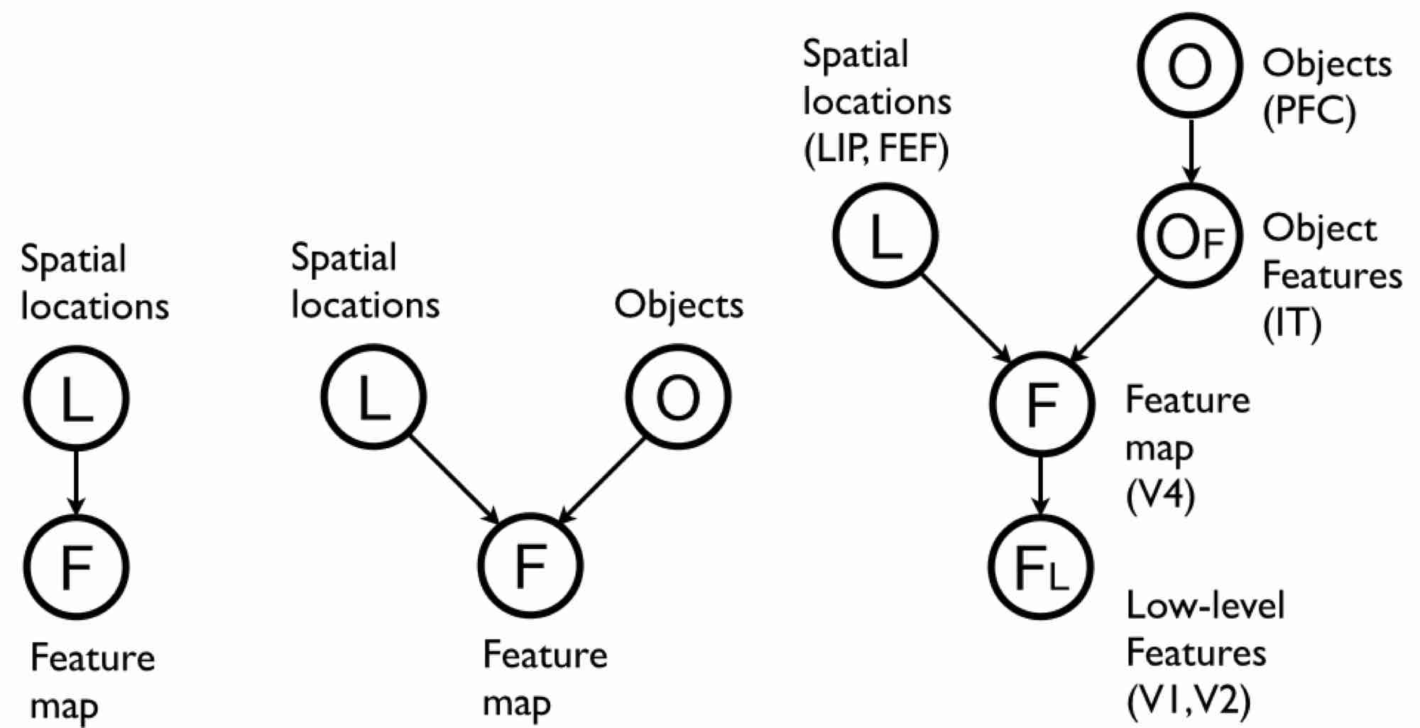
Figure 10: PGMs of increasing level of representational complexity (left to right) that can account for most models proposed in the computational vision field. Left: feature-based model. Centre: object-based model. Right: the Bayesian model by Chikkerur et al. Poggio2010 , which extends the object-based model in the centre and maps the resulting PGM structure to brain areas underpinning visual attention: early visual areas V1 and V2, V4, lateral intraparietal (LIP), frontal eye fields (FEF), inferotemporal (IT), prefrontal cortex (PFC).

As it can be seen, it is a subgraph of the object-based model PGM (Fig. 10, centre), which is the one previously discussed in Box 5.

Surprisingly enough, this simple model is sufficiently powerful to account for a large number of visual attention models that have been proposed in computational vision. This can be easily appreciated by setting $P(\mathbf{F}\mid\mathbf{L})=const.,P(\mathbf{L})=const.$ so that Eq. 14 reduces to

$$\overbrace{P(\mathbf{L}\mid\mathbf{F})}^{\text{posterior prob. of selecting location L }}\propto\overbrace{\frac{1}{P(\mathbf{F})}}^{\text{salience at location L}}.$$ (15)

Eq. 15 tells that the probability of fixating a spatial location $\mathbf{L}=(x,y)$ is higher when “unlikely” features ($\frac{1}{P(\mathbf{F})}$) occur at that location. In a natural scene, it is typically the case of high contrast regions (with respect to either luminance, color, texture or motion) and clearly relates to entropy and information theory concepts BocICIAP2001 . This is nothing but the most prominent salience-based model in the literature proposed by Itti et al IttiKoch98 , which Eq. 15 only re-phrases in probabilistic terms.

A thorough reading of the recent review by Borji and Itti BorItti2012 is sufficient to gain the understanding that a great deal computational models so far proposed are more or less variations of this leitmotif (experimenting with different features, different weights for combining them, etc.). The weakness of such a pure bottom-up approach has been largely discussed (see, e.g. TatlerBallard2011eye ; foulsham2008 ; EinhauserSpainPerona2008 ). Indeed, the effect of early saliency on attention is likely to be a correlational effect rather than an actual causal one foulsham2008 ; schutz2011eye , though salience may be still more predictive than chance while preparing for a memory test as discussed by Foulsham and Underwood foulsham2008 .

Thus, recent efforts have tried to go beyond this simple stage with the aim of climbing the representational hierarchy shown in Fig. 2. This entails a first shift from Eq. 15 (based on an oversimplified representation) back to Eq. 14. Torralba et al. Torralba have shown that using prior knowledge on the typical spatial location of the search target, as well as contextual information (the “gist” of a scene) to modulate early saliency improves its fixation prediction.

Next shift is exploiting object knowledge for top-down “tuning” early salience; thus, moving to the PGM representation at the centre of Figure 10. Indeed, objects and their semantic value have been deemed as fundamental for visual attention and eye guidance (e.g., mozer1987 ; bundesen1998 ; rensink2000dynamic ; heinke2011modelling , but see Scholl scholl for a review). For instance, when dealing with faces within the scene, a face detection step can provide a reliable cue to complement early conspicuity maps, as it has been shown by Cerf et al cerf2008predicting , deCroon et al postma2011 , Marat et al marat2013improving , or a useful prior for Bayesian integration with low level cues bocc08tcsvt . This is indeed an important issue since faces may drive attention in a direct fashion cerf2009faces . The same holds for text regions cerf2008predicting ; BocCOGN2014 Other notable exceptions are those provided by Rao et al. Rao2002 , Sun et al. Sun2008 , the Bayesian models discussed by Borji et al. borji2012object and Chikkerur et al. Poggio2010 . In particular the model by Chikkerur et al., which is shown at right of Fig. 10 is the most complete to the best of our knowledge (though it does not consider contextual scene information Torralba , but the latter could be easily incorporated). Interestingly enough, the authors have the merit of making the effort of providing links between the structure of the PGM and the brain areas that could support computations.

Further, again in the effort of climbing the representational hierarchy (Fig. 2), attempts have been made for incorporating task and value information (see BocCOGN2014 ; schutz2011eye for a brief review, and TatlerBallard2011eye for a discussion).

Now, a simple question arises: where have the eye movements gone?

To answer such question is useful to summarise the brief overview above. The common practice of computational approaches is to conceive the mapping (1), as a two step procedure:

1. obtain a suitable representation $\mathcal{R}$, i.e., $\mathcal{D}\xmapsto[\mathbf{T}]{}\mathcal{R}$;

2. use $\mathcal{R}$ to generate the scanpath, $\mathcal{R}\xmapsto[\mathbf{T}]{}\{\mathbf{x}_{F}(1),\mathbf{x}_{F}(2),\cdots\}$.

Computational modelling has been mainly concerned with the first step: deriving a representation $\mathcal{R}$ (either probabilistic or not). The second step, that is $\mathcal{R}\mapsto\{\mathbf{x}_{F}(1),\mathbf{x}_{F}(2),\cdots\}$, which actually brings in the question of how we look rather than where, is seldom taken into account.

In spite of the fact that the most cited work in the field, that by Itti et al IttiKoch98 , clearly addressed the how issue (gaze shifts as the result of a Winner-Take-All, WTA, sequential selection of most salient locations), most models simply overlook the eye movement problem. The computed representation $\mathcal{R}$ is usually evaluated in terms of its capacity for predicting the image regions that will be explored by covert and overt attentional shifts according to some evaluation measure BorItti2012 . In other cases, if needed for practical purposes, e.g. for robotic applications, the problem of oculomotor action selection is solved by adopting some deterministic choice procedure. These usually rely on selecting the gaze position $\mathbf{x}$ as the argument that maximises a measure on the given representation $\mathcal{R}$ (in brief, see walther2006 for using the $\arg\max_{\mathbf{x}}\mathcal{R}$ operation and BocFerSMCB2013 ; TatlerBallard2011eye , for an in-depth discussion).

Yet, another issue arises: the variability of visual scan paths. When looking at natural movies under a free-viewing or a general-purpose task, the relocation of gaze can be different among observers even though the same locations are taken into account. In practice, there is a small probability that two observers will fixate exactly the same location at exactly the same time. Such variations in individual scan paths (as regards chosen fixations, spatial scanning order, and fixation duration) still hold when the scene contains semantically rich ”objects” (e.g., faces, see Fig. 1). Variability is even exhibited by the same subject along different trials on equal stimuli. Further, the consistency in fixation locations between observers decreases with prolonged viewing dorr2010variability . This effect is remarkable when free-viewing static images: consistency in fixation locations selected by observers decreases over the course of the first few fixations after stimulus onset TatlerBallard2011eye and can become idiosyncratic.

Note that, the WTA scheme IttiKoch98 ; walther2006 , or the selection of the proto-object with the highest attentional weight anna are deterministic procedures. Even when probabilistic frameworks are used to infer where to look next, the final decision is often taken via the maximum a posteriori (MAP) criterion, which again is an $\arg\max$ operation (e.g., elazary2010bayesian ; bocc08tcsvt ; geisler2005 ; ChernyakStark ), or variants such as the robust mean (arithmetic mean with maximum value) over candidate positions begum2010probabilistic . As a result, for a chosen visual data input $\mathcal{D}$ the mapping $\mathcal{R}\xmapsto[\mathbf{T}]{}\{\mathbf{x}_{F}(1),\mathbf{x}_{F}(2),\cdots\}$ will always generate the same scanpath across different trials.

There are few notable exceptions to this current state of affairs (see BocFerSMCB2013 for a discussion). In kimura2008dynamic simple eye-movement patterns, in the vein of tatler2009prominence , are straightforwardly incorporated as a prior of a dynamic Bayesian network to guide the sequence of eye focusing positions on videos. The model presented in ho2009computational embeds at least one parameter suitable to be tuned to obtain different saccade length distributions on static images, although statistics obtained by varying such parameter are still far from those of human data. The model by Keech and Resca keech2010eye1 mimics phenomenologically the observed eye movement trajectories and where randomness is captured through a Monte Carlo selection of a particular eye movement based on its probability; probabilistic modelling of eye movement data has been also discussed in rutishauser2007probabilistic . However, both models address the specific task of conjunctive visual search and are limited to static scenes. Other exceptions are given, but in the very peculiar field of eye-movements in reading feng2006eye . Other works have addressed the variability issue in the framework of foraging random walks bfpha04 ; BocFerSMCB2013 ; BocFerAnnals2012 ; BocFerSPIC2012 ; BocCOGN2014 ; napboc_TIP2015 .

What we need at least is to bring stochasticity back into the game. As Canosa put it canosa2009real :

Where we choose to look next at any given moment in time is not completely deterministic, yet neither is it completely random.

5 Stochastic processes and eye movements

When we randomly sample a sequence $\{\mathbf{x}(t=1),\mathbf{x}(t=2),\mathbf{x}(t=3),\cdots\}$ of gaze shifts from the pdf $P(\mathbf{x})$ (cfr., Eq.8), we set up a stochastic process. For example, the ensemble of different scan paths on the same viewed image can be conceived as the record of a stochastic process (Fig. 11)

t]

Figure 11: An ensemble of scan paths recorded from different observers while viewing the same image. For visualisation purposes, only five trajectories are shown, different colors coding individual trajectories. If such ensemble is considered to represent the outcome of a stochastic process, the fundamental question that should be answered is: What is the probability $P(\mathbf{x},t)$ of gazing at location $\mathbf{x}$ at time $t$? Images and data are from the Doves dataset van2009doves

Stochastic processes are systems that evolve probabilistically in time or more precisely, systems in which a certain time-dependent random variable $\mathbf{X}(t)$ exists (as to notation, we may sometimes write $\mathbf{X}_{t}$ instead of $\mathbf{X}(t)$) The variable $t$ usually denotes time and it can be integer or real valued: in the first case, $\mathbf{X}(t)$ is a discrete time stochastic process; in the second case, it is a continuous time stochastic process. We can observe realisations of the process, that is we can measure values

$$\mathbf{X}(t_{1})=\mathbf{x}_{1},\;\;\mathbf{X}(t_{2})=\mathbf{X}_{2},\;\;\mathbf{X}(t_{3})=\mathbf{x}_{3},\cdots,$$

at times $t_{1},t_{2},t_{3},\cdots$. The set $\mathcal{S}$ whose elements are the values of the process is called state space.

Thus, we can conceive the stochastic process $\mathbf{X}(t)$ as an ensemble of paths as shown in Fig. 3 or, more simply, as illustrated in Fig. 12: here, for concreteness, we show four series of the raw $x$ coordinates of different eye-tracked subjects gazing at picture shown in Fig. 3. Note that if we fix the time, e.g., $t=t_{1}$, then $\mathbf{X}(t_{1})$ boils down to a RV (vertical values); the same holds if we choose one path $\mathbf{x}$ and we (horizontally) consider the set of values $\mathbf{x}_{1},\;\;\mathbf{x}_{2},\;\;\mathbf{x}_{3},\cdots,$ at times $t_{1},t_{2},t_{3},\cdots$.

To sum up, a stochastic process can be regarded as either a family of realisations of a random variable in time, or as a family of random variables at fixed time. Interestingly enough, referring back to Section 3, notice that Einstein’s point of view was to treat Brownian motion as a distribution of a random variable describing position, while Langevin took the point of view that Newton’s law’s of motion apply to an individual realisation.

t]

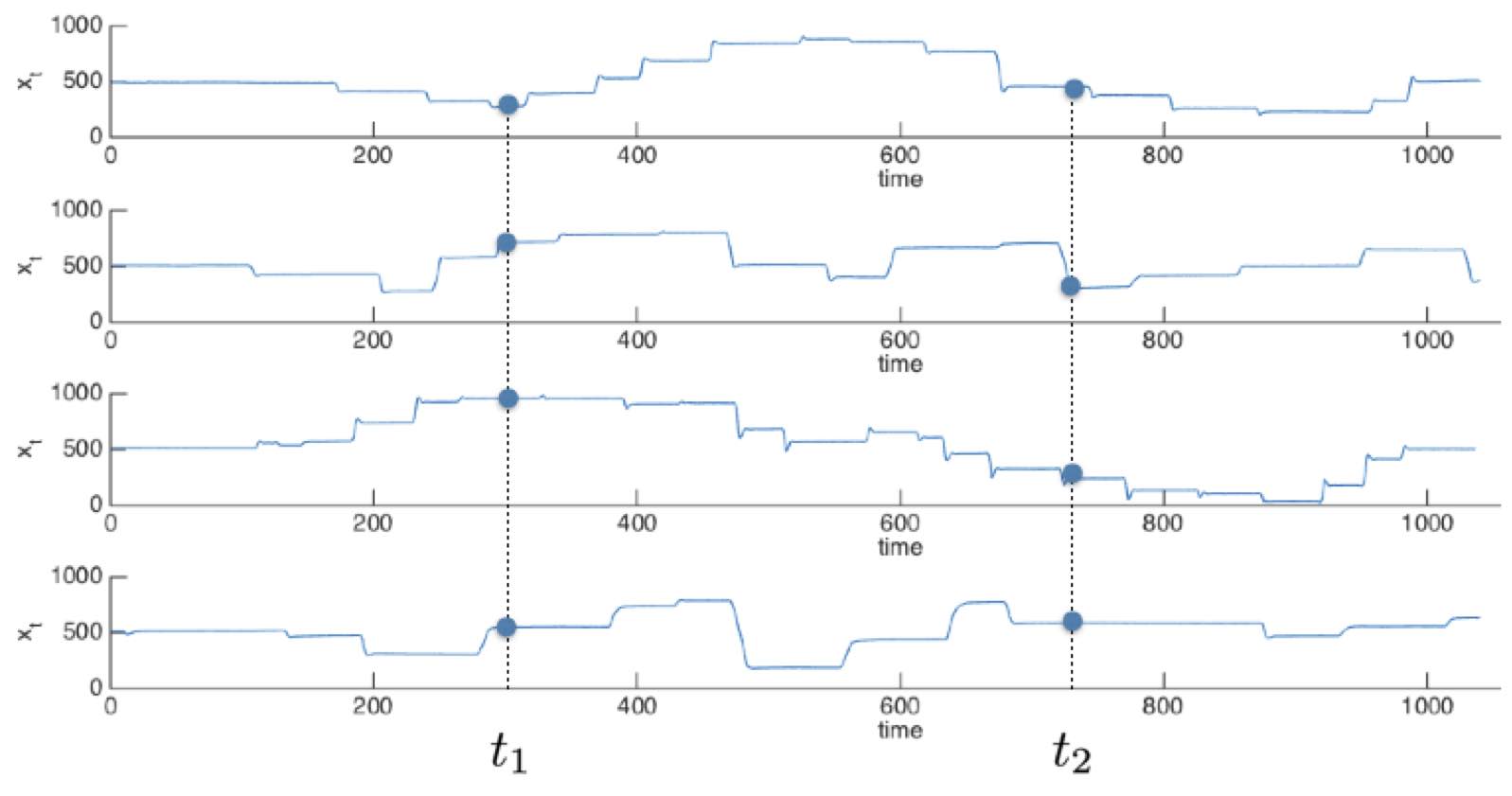
Figure 12: An ensemble of paths representing a stochastic process. Each path represents the sequence in time of raw $x$ coordinates from different scan paths recorded on the same picture (cfr. Fig. 11). We can conceive the trajectories (namely, time series) of such ensemble as realisations of a stochastic process.

In order to be more compact with notation, we will use Huang’s abbreviation huang2001introduction

$$k\leftrightarrow\{\mathbf{x}_{k},t_{k}\},$$

where, e.g., $P(1)$ succintly stands for $P(\mathbf{x}_{1},t_{1})$.

To describe the process completely we need to know the correlations in time, that is the hierarchy of pdfs (but see Box 6, for a discussion of correlation):

$$P(1):\text{ the 1 point pdf}$$ (16)

$$P(1,2):\text{ the 2 points pdf}$$

$$\ P(1,2,3):\text{ the 3 points pdf}$$

$$\ \cdots$$

up to the $n$ point joint pdf. The $n$ point joint pdf must imply all the lower $k$ point pdfs, $k<n$:

$$P(1,\cdots,k)=\int P(1,\cdots,n)d\mathbf{x}_{k+1}d\mathbf{x}_{k+2}\cdots d\mathbf{x}_{n}$$ (17)

where $P(1,\cdots,n)d\mathbf{x}_{k+1}d\mathbf{x}_{k+2}\cdots d\mathbf{x}_{n}$ stands for the joint probability of finding that $\mathbf{x}$ has a certain value

$\mathbf{x}_{k+1}<\mathbf{x}\leq\mathbf{x}_{k+1}+d\mathbf{x}_{k+1}$ at time $t_{k+1}$

$\mathbf{x}_{k+2}<\mathbf{x}\leq\mathbf{x}_{k+2}+d\mathbf{x}_{k+2}$ at time $t_{k+2}$

$\cdots$

Table 6: How to observe a stochastic process

Consider a series of time signals. The signal fluctuates up and down in a seemingly erratic way. The measurements that are in practice available at one time of a measurable quantity $x(t)$ are the mean and the variance. However, the latter do not tell a great deal about the underlying dynamics of what is happening. A fundamental question in time series analysis is: to what extent the value of a RV variable measured at one time can be predicted from knowledge of its value measured at some earlier time? Does the signal at $t_{0}$ influence what is measured at a later time $t_{0}+t$? We are not interested in any specific time instant $t_{0}$ but rather in the typical (i.e., the statistical) properties of the fluctuating signal. The amount of dependence, or history in the signal can be characterised by the autocorrelation function

$$C_{xx}(\tau)=\lim_{T\to\infty}\frac{1}{T}\int_{0}^{T}x(t)x(t+\tau)dt.$$ (18)

This is the time average of a two-time product over an arbitrary large time $T$, which is then allowed to become infinite. Put simply, is the integral of the product of the time series with the series simply displaced with respect to itself by an amount $\tau$. An autocorrelated time series is predictable, probabilistically, because future values depend on current and past values. In practice, collected time series are of finite length, say $N$. Thus, the estimated autocorrelation function is best described as the sample autocorrelation

$$c_{xx}(\Delta)=\frac{1}{N}\sum_{n=0}^{N-|\Delta|-1}x(n)x(n+\Delta)$$ (19)

Measurements of $C_{xx}(\tau)$ are used to estimate the time-dependence of the changes in the joint probability distribution, where the lag is $\tau=t-t_{0}$. If there is no statistical correlation $C_{xx}(\tau)=0$. The rate at which $C_{xx}(\tau)$ approaches $0$ as $\tau$ approaches $\infty$ is a measure of the memory for the stochastic process, which can also be defined in terms of correlation time:

$$t_{corr}=\frac{1}{C_{xx}(0)}\int_{0}^{+\infty}C_{xx}(\tau)d\tau.$$ (20)

The autocorrelation function has been defined so far as a time average of a signal, but we may also consider the ensemble average, in which we repeat the same measurement many times, and compute averages, denoted by symbol $\langle\rangle$. Namely, the correlation function between $x(t)$ at two different times $t_{1}$ and $t_{2}$ is given by

$$\langle x(t_{1}),x(t_{2})\rangle=\int_{-\infty}^{+\infty}\int_{-\infty}^{+\infty}x_{1}x_{2}P(x_{1},t_{1};x_{2},t_{2})dx_{1}dx_{2}.$$ (21)

For many systems the ensemble average is equal to the time average, $\langle x\rangle=\int_{-\infty}^{+\infty}x_{1}P(x_{1},t)dx_{1}\approx\lim_{T\to\infty}\frac{1}{T}\int_{0}^{T}x(t)dt=\overline{x(t)}$. Such systems are termed ergodic. Ergodic ensembles for which the probability distributions are invariant under time translation and only depend on the relative times $t_{2}-t_{1}$ are stationary processes. If we have a stationary process, it is reasonable to expect that average measurements could be constructed by taking values of the variable $x$ at successive times, and averaging various functions of these. Correlation and memory properties of a stochastic process are typically investigated by analysing the autocorrelation function or the spectral density (power spectrum) $S(\omega)$, which describes how the power of a time series is distributed over the different frequencies. These two statistical properties are equivalent for stationary stochastic processes. In this case the Wiener-Kintchine theorem holds

$$S(\omega)=\frac{1}{2\pi}\int_{-\infty}^{-\infty}\exp{(-i\omega\tau)}C_{xx}(\tau)d\tau$$ (22)

$$C_{xx}(\tau)=\int_{-\infty}^{-\infty}\exp{(i\omega\tau)}S(\omega)d\omega$$ (23)

It means that one may either directly measure the autocorrelation function of a signal, or the spectrum, and convert back and forth, which by means of the Fast Fourier Transform (FFT) is relatively straightforward. The sample power spectral density function is computed via the FFT of $c_{xx}$, i.e. $s(\omega)=FFT(c_{xx}(\Delta))$, or viceversa by the inverse transform, $c_{xx}(\Delta=IFFT(s(\omega))$.

For instance, referring to Fig. 12, we can calculate the joint probability $P(1,2)d\mathbf{x}_{1}d\mathbf{x}_{2}$ by following the vertical line at $t_{1}$ and $t_{2}$ and find the fraction of paths for which $\mathbf{x}(t_{1})=\mathbf{x}_{1}$ within tolerance $d\mathbf{x}_{1}$ and $\mathbf{x}(t_{2})=\mathbf{x}_{2}$ within tolerance $d\mathbf{x}_{2}$, respectively

Summing up, the joint probability density function, written in full notation as

$$P(\mathbf{x}_{1},t_{1};\mathbf{x}_{2},t_{2};\cdots;\mathbf{x}_{n},t_{n}),$$

is all we need to fully characterise the statistical properties of a stochastic process and to calculate the quantities of interest characterising the process (see Box 6).

The dynamics, or evolution of a stochastic process can be represented through the specification of transition probabilities:

$P(2\mid 1)$ : probability of finding $2$, when $1$ is given;

$P(3\mid 1,2)$ : probability of finding $3$, when $1$ and $2$ are given;

$P(4\mid 1,2,3)$ : probability of finding $4$, when $1,2$ and $3$ are given;

$\cdots$

Transition probabilities for a stochastic process are nothing but the conditional probabilities suitable to predict the future values of $\mathbf{X}(t)$ (i.e., $\mathbf{x}_{k+1},\mathbf{x}_{k+2},\cdots\mathbf{x}_{k+l}$, at $t_{k+1},t_{k+2},\cdots t_{k+l}$), given the knowledge of the past ($\mathbf{x}_{1},\mathbf{x}_{2},\cdots\mathbf{x}_{k}$, at $t_{1},t_{2},\cdots t_{k}$). The conditional pdf explicitly defined in terms of the joint pdf can be written:

$$P(\overbrace{\mathbf{x}_{k+1},t_{k+1};\cdots;\mathbf{x}_{k+l},t_{k+l}}^{\text{future}}\mid\underbrace{\mathbf{x}_{1},t_{1};\cdots;\mathbf{x}_{k},t_{k}}_{\text{past}})=\frac{P(\mathbf{x}_{1},t_{1};\cdots;\mathbf{x}_{k+l},t_{k+l})}{P(\mathbf{x}_{1},t_{1};\cdots;\mathbf{x}_{k},t_{k})}.$$ (24)

assuming the time ordering $t_{1}<t_{2}<\cdots<t_{k}<t_{k+1}<\cdots<t_{k+l}$.

By using transition probabilities and the product rule, the following update equations can be written:

$$P(1,2) = P(2\mid 1)P(1)$$ (25)

$$P(1,2,3) = P(3\mid 1,2)P(1,2)$$

$$P(1,2,3,4) = P(4\mid 1,2,3)P(1,2,3)$$

$$\cdots$$

The transition probabilities must satisfy the normalisation condition $\int P(2\mid 1)d\mathbf{x}_{2}=1$. Since $P(2)=\int P(1,2)d\mathbf{x}_{1}$ and by using the update Eqs. (25), the following evolution (integral) equation holds

$$P(2)=\int\overbrace{P(2\mid 1)}^{\text{propagator}}P(1)d\mathbf{x}_{1}$$ (26)

where $P(2\mid 1)$ serves as the evolution kernel or propagator from state $1$ to state $2$, i.e., in full notation, from state $(\mathbf{x}_{1},t_{1})$ to state $(\mathbf{x}_{2},t_{2})$.

A stochastic process whose joint pdf does not change when shifted in time is called a (strict sense) stationary process:

$$P(\mathbf{x}_{1},t_{1};\mathbf{x}_{2},t_{2};\cdots;\mathbf{x}_{n},t_{n})=P(\mathbf{x}_{1},t_{1}+\tau;\mathbf{x}_{2},t_{2}+\tau;\cdots;\mathbf{x}_{n},t_{n}+\tau)$$ (27)

$\tau>0$ being a time shift. Analysis of a stationary process is frequently much simpler than for a similar process that is time-dependent: varying $t$, all the random variables $\mathbf{X}_{t}$ have the same law; all the moments, if they exist, are constant in time; the distribution of $\mathbf{X}(t_{1})$ and $\mathbf{X}(t_{2})$ depends only on the difference $\tau=t_{2}-t_{1}$ (time lag), i.e,

$$P(\mathbf{x}_{1},t_{1};\mathbf{x}_{2},t_{2})=P(\mathbf{x}_{1},\mathbf{x}_{2};\tau).$$

A conceptual map of main kinds of stochastic processes that we will discuss in the remainder of this Chapter is presented in Fig. 13.

t] .

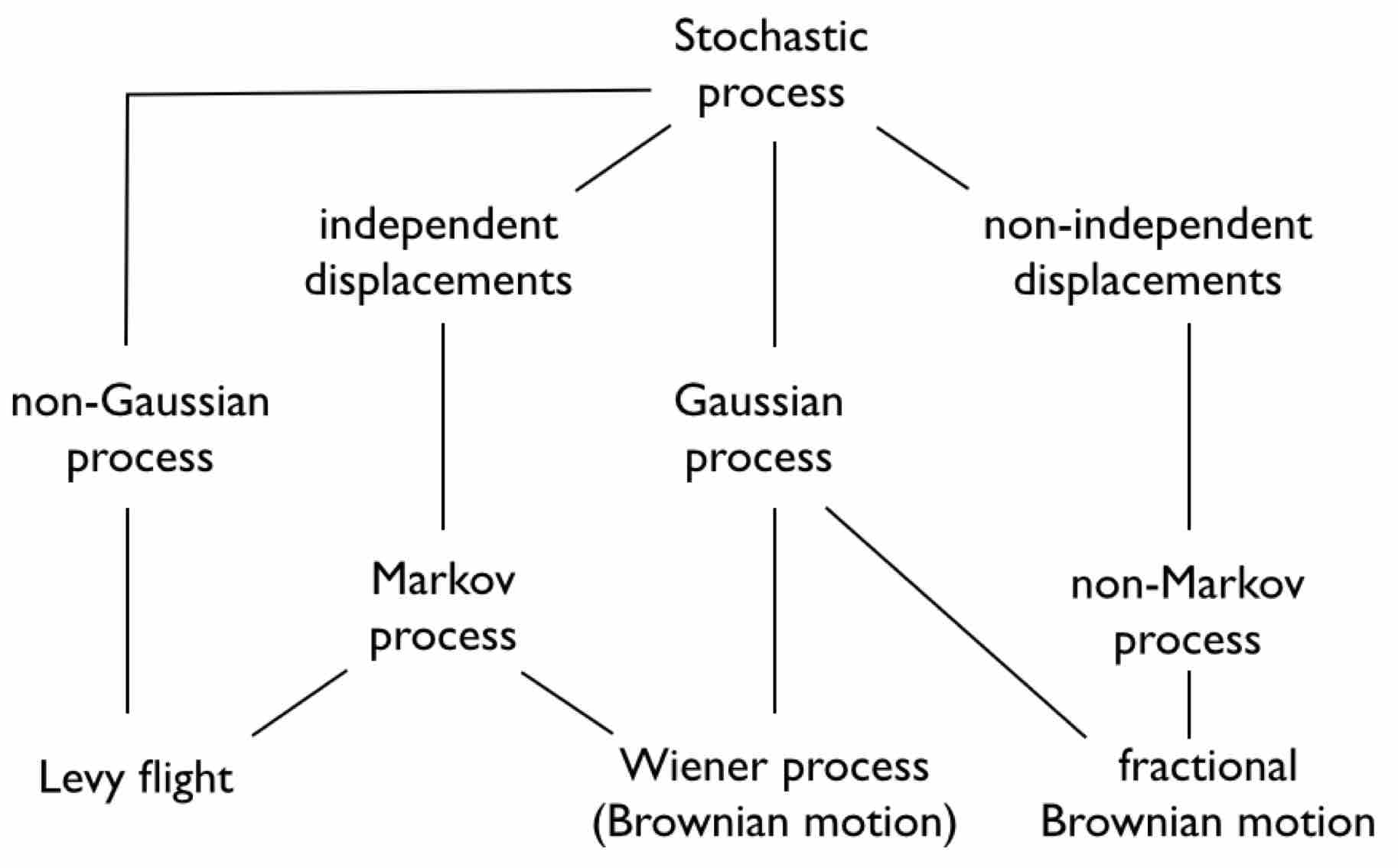
Figure 13: A conceptual map of stochastic processes that are likely to play a role in eye movement modelling and analyses

6 How to leave the past behind: Markov Processes

The most simple kind of stochastic process is the Purely Random Process in which there are no correlations. From Eq. (25):

$$P(1,2) = P(1)P(2)$$ (28)

$$P(1,2,3) = P(1)P(2)P(3)$$

$$P(1,2,3,4) = P(1)P(2)P(3)P_{1}(3)$$

$$\cdots$$

One such process can be obtained for example by repeated coin tossing. The complete independence property can be written explicitly as:

$$P(\mathbf{x}_{1},t_{1};\mathbf{x}_{2},t_{2};\cdots)=\prod_{i}P(\mathbf{x}_{i},t_{i}),$$ (29)

the uppercase greek letter $\prod$ indicates a product of factors, e.g., for $i=1,2,3$, $P(\mathbf{x}_{1},t_{1};\mathbf{x}_{2},t_{2};\mathbf{x}_{3},t_{3})=P(\mathbf{x}_{1},t_{1})P(\mathbf{x}_{2},t_{2})P(\mathbf{x}_{3},t_{3})$.

Equation 29 means that the value of $\mathbf{X}$ at time $t$ is completely independent of its values in the past (or future). A special case occurs when the $P(\mathbf{x}_{i},t_{i})$ are independent of $t$, so that the same probability law governs the process at all times. Thus, a completely memoryless stochastic process is composed by a set of independent and identically distributed (i.i.d) RVs. Put simply, a series of i.i.d. RVs is a series of samples where individual samples are “independent” of each other and are generated from the same probability distribution (“identically distributed”).

More realistically, we know that most processes in nature, present some correlations between consecutive values. For example, the direction of the following gaze shift is likely to be positively correlated with the direction of current gaze shift. A step towards a more realistic description consists then of assuming that the next value of each RV in the process depends explicitly on the current one (but not explicitly on any other previous to that). An intuitive example is the simple random walk, which is briefly discussed in Box 7, and can be modelled by the simple equation

$$x_{t}=x_{t-1}+\xi_{t},$$ (30)

where the noise term $\xi_{t}$ is sampled, at each step $t$, from a suitable distribution $P(\xi)$.

Note that if we iterate Eq. (30) for a number of steps $t=1,2,3,\cdots$ and collect the output sequence of the equation, that is $x_{1},x_{2},x_{3},\cdots$, we obtain a single trajectory/path of the walk, which is one possible realisation of the underlying stochastic process. This corresponds to consider one horizontal slice of Fig. 12, that is a (discrete) time series. It is worth mentioning that there exist a vast literature on time series analysis, which can be exploited in neuroscience data analysis and more generally in other fields. Indeed, the term “time series” more generally refers to data that can be represented as a sequence. This includes for example financial data in which the sequence index indicates time, as in our case, but also genetic data (e.g. ACATGC . . .) where the sequence index has no temporal meaning. Some of the methods that have been developed in this research area might be useful for eye movement modelling and analysis. We have no place here to further discuss this issue, however Box 8 provides some “pointers” for the reader.

Table 7: Random walks

Random walks (RW) are a special kind of stochastic process and can be used, as we will see, to model the dynamics of many complex systems. A particle moving in a field, an animal foraging, and indeed the “wandering” eye can be conceived as examples of random walkers.

In general, RWs exhibit what is called serial correlation, conditional independence for fairly small values of correlation length $t_{corr}$ (cfr., Box 6, Eq. 20), and a simple stochastic historical dependence. For instance, a simple additive $1-$dimensional random walk has the form:

$$x_{t}=x_{t-1}+\xi_{t},\text{ where }\xi_{t}\sim P(\xi)$$ (31)

In the above formulation, time $t$ proceeds in discrete steps. $\xi_{t}$ is a RV drawn i.i.d. from a distribution $P(\xi)$, called the noise or fluctuation distribution. Thus, the differences in sequential observations $x_{t}-x_{t-1}=\xi_{t}\sim P(\xi)$ are i.i.d. We have here independent displacements.

However, the observations themselves are not independent, since (31) encodes the generative process, or evolution law, $x_{t-1}\rightarrow x_{t}$ where $x_{t}$ explicitly depends on $x_{t-1}$, but not on earlier $x_{t-2},x_{t-3},x_{t-4},\cdots$. Thus Eq. (31) represents a Markov process.

Conventionally, fluctuations are Gaussian distributed with mean $\mu$ and variance $\sigma^{2}$, that is, $\xi\sim\mathcal{N}(\mu,\sigma^{2})$, as this makes mathematical analysis considerably simpler. In this case by simply extending to two dimensions Eq. 31,

$$x_{t}=x_{t-1}+\xi_{x,t}$$ (32)

$$y_{t}=y_{t-1}+\xi_{y,t},$$

the simulation of a simple Brownian RW can be obtained (see Fig. 14).

However, any probability distribution, for instance, a Laplace (exponential tails) or double-Pareto distribution (power-law tails), also works.

Table 8: As time goes by: time series analysis

The random walk model summarised by Eq. 30, can be seen as a special case of the model

$$x_{t}=\alpha_{1}x_{t-1}+\xi_{t},$$ (33)

with model parameter $\alpha_{1}=1$.

In time series analysis, under the assumption that $\xi_{t}$ is sampled from a Gaussian distribution mean zero and variance $\sigma^{2}$, the model specified by Eq. 33 is known as an autoregressive or AR model of order $1$, abbreviated to AR($1$).

The AR($1$) model, in turn is a special case of an autoregressive process of order $p$, denoted as AR($p$):

$$x_{t}=\alpha_{1}x_{t-1}+\alpha_{2}x_{t-2}+\cdots+\alpha_{p}x_{t-p}+\xi_{t},$$ (34)

with model parameters $\alpha_{p}\neq 0$. Note that such model is a regression of $x_{t}$ on past terms from the same series; hence the use of the term “autoregressive”.

Considering again the RW of Eq. 30. One can substitute the term $x_{t-1}$, that by using the same equation can be calculated as $x_{t-1}=x_{t-2}+\xi_{t-1}$; thus,

$$x_{t}=x_{t-2}+\xi_{t-1}+\xi_{t}.$$ (35)

Continuing and substituting for $x_{t-2}$, followed by $x_{t-3}$ and so on (a process known as “back substitution”) gives

$$x_{t}=\xi_{1}+\xi_{1}+\cdots+\xi_{t-1}+\xi_{t},$$ (36)

where $x_{t}$ is written as the sum of the current noise term $\xi_{t}$ and the past noise terms.

This result can be generalised by writing $x_{t}$ as the linear combination of the current white noise term and the $q$ most recent past noise terms

$$x_{t}=\xi_{t}+\beta_{1}\xi_{t-1}+\beta_{2}\xi_{t-2}+\cdots+\beta_{q}\xi_{t-q}.$$ (37)

This defines a moving average or MA model of order $q$, shortly MA($q$).

Putting all together, we can write the general expression:

$$x_{t}=\alpha_{1}x_{t-1}+\alpha_{2}x_{t-2}+\cdots+\alpha_{p}x_{t-p}+\xi_{t}+\beta_{1}\xi_{t-1}+\beta_{2}\xi_{t-2}+\cdots+\beta_{q}\xi_{t-q}.$$ (38)

The time series is said to follow an autoregressive moving average or ARMA model of order $(p,q)$, denoted ARMA($p,q$).

By expanding on the former, a great deal of models can be conceived. Also, a variety of methods, algorithms, and related software, is at hand for estimating the model parameters from time series data. Cowpertwait and Metcalfe metcalfe2009introductory provide a thorough introduction with R language examples, for R fans. The book edited by Barber, Cemgil and Chiappa barber2011bayesian offers a comprehensive picture of modern time series techniques, specifically those based on Bayesian probabilistic modelling. Time series modelling is a fast-growing trend in neuroscience data analysis, which is addressed in-depth by Ozaka ozaki2012time .

Going back to stochastic processes, if a process has no memory beyond the last transition then it is called a Markov process and the transition probability enjoys the property:

$$P(\mathbf{x}_{n},t_{n}|\mathbf{x}_{n-1},t_{n-1};\cdots;\mathbf{x}_{1},t_{1})=P(\mathbf{x}_{n},t_{n}|\mathbf{x}_{n-1},t_{n-1})$$ (39)

with $t_{1}<t_{2}<\cdots<t_{n}$.

A Markov process is fully determined by the two densities $P(\mathbf{x}_{1},t_{1})$ and $P(\mathbf{x}_{2},t_{2}\mid\mathbf{x}_{1},t_{1})$; the whole hierarchy can be reconstructed from them. For example, from Eq. (25) using the Markov property $P(3\mid 1,2)=P(3\mid 2)$:

$$P(1,2,3)=P(1)P(2\mid 1)P(3\mid 2).$$ (40)

The factorisation of the joint pdf can thus be explicitly written in full notation as

$$P(\mathbf{x}_{n},t_{n};\mathbf{x}_{n-1},t_{n-1};\cdots;\mathbf{x}_{1},t_{1})=P(\mathbf{x}_{1},t_{1})\prod_{i=2}^{n}P(\mathbf{x}_{i},t_{i}\mid\mathbf{x}_{i-1},t_{i-1}),$$ (41)

with the propagator $P(\mathbf{x}_{i+1},t_{i+1}\mid\mathbf{x}_{i},t_{i})$ carrying the system forward in time, beginning with the initial distribution $P(\mathbf{x}_{1},t_{1})$.

A well known example of Markov process is the Wiener-Lévy process describing the position of a Brownian particle (Fig.14).

t]

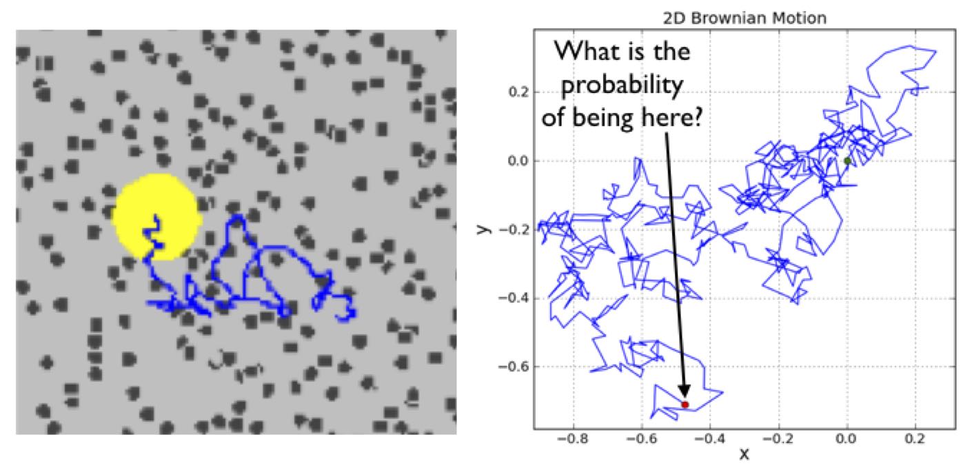
Figure 14: Motion of a Brownian particle. Left: The physical mechanism of the displacement (in blue): the bigger particle performs a Brownian motion (Bm) as a result of the collisions with small particles (figure is not to scale). Right: Sample path of the Bm performed by the bigger particle. Here the fundamental question is: What is the probability of the particle being at location $\mathbf{x}=(x,y)$ at time $t$? (cfr. Box 9)

The fact that a Markov process is fully determined by $P(1)$ and $P(2\mid 1)$ does not mean that such two functions can be chosen arbitrarily, for they must also obey two important identities.

The first one is Eq. (26) that in explicit form reads:

$$P(\mathbf{x}_{2},t_{2})=\int_{\mathbf{x}_{1}}P(\mathbf{x}_{2},t_{2}\mid\mathbf{x}_{1},t_{1})P(\mathbf{x}_{1},t_{1})d\mathbf{x}_{1}.$$ (42)

This equation simply constructs the one time probabilities in the future $t_{2}$ of $t_{1}$, given the conditional probability $P(\mathbf{x}_{2},t_{2}\mid\mathbf{x}_{1},t_{1})$.

The second property can be obtained by marginalising the joint pdf $P(\mathbf{x}_{3},t_{3},\mathbf{x}_{2},t_{2}\mid\mathbf{x}_{1},t_{1})$ with respect to $\mathbf{x}_{2}$ and by using the definition of conditional density under the Markov property:

$$P(\mathbf{x}_{3},t_{3}\mid\mathbf{x}_{1},t_{1})=\int_{\mathbf{x}_{2}}P(\mathbf{x}_{3},t_{3}\mid\mathbf{x}_{2},t_{2})P(\mathbf{x}_{2},t_{2}\mid\mathbf{x}_{1},t_{1})d\mathbf{x}_{2},$$ (43)

Equation (43) is known as the Chapman-Kolmogorov Equation (C-K equation, from now on). It is “just” a statement saying that to move from position $\mathbf{x}_{1}$ to $\mathbf{x}_{3}$ you just need to average out all possible intermediate positions $\mathbf{x}_{2}$ or, more precisely, by marginalisation over the nuisance variable $\mathbf{x}_{2}$.

t]

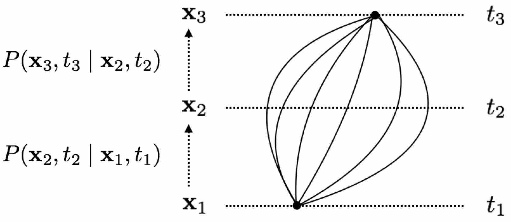
Figure 15: The Chapman-Kolmogorov equation at work: the probability of transition from the event $(\mathbf{x}_{1},t_{1})$ to $(\mathbf{x}_{3},t_{3})$ is broken into a subprocess from $(\mathbf{x}_{1},t_{1})$ to an intermediate, nuisance event $(\mathbf{x}_{2},t_{2})$ (which is not observed in practice) and then from $(\mathbf{x}_{2},t_{2})$ to $(\mathbf{x}_{3},t_{3})$, by considering all the paths from $\mathbf{x}_{1}$ to $\mathbf{x}_{3}$.

Such equation is a consistency equation for the conditional probabilities of a Markov process and the starting point for deriving the equations of motion for Markov processes. Aside from providing a consistency check, the real importance of the C-K equation is that it enables us to build up the conditional probability densities over the “long” time interval $[t_{1},t_{3}]$ from those over the “short” intervals $[t_{1},t_{2}]$ and $[t_{2},t_{3}]$.

The C-K equation is a rather complex nonlinear functional equation relating all conditional probabilities $P(\mathbf{x}_{i},t_{i}\mid\mathbf{x}_{j},t_{j})$ to each other. Its solution would give us a complete description of any Markov process, but unfortunately, no general solution to this equation is known: in other terms, it expresses the Markov character of the process, but containing no information about any particular Markov process.

The idea of forgetting the past so to use the present state for determining the next one might seem an oversimplified assumption when dealing, for instance, with eye movements performed by an observer engaged in some overt attention task. However, this conclusion may not in fact be an oversimplification. This was discussed by Horowitz and Wolfe horowitz1998visual , and will be detailed in the following subsection.

6.1 Case study: the Horowitz and Wolfe hypothesis of amnesic visual search

Serial and parallel theories of visual search have in common the memory-driven assumption that efficient search is based on accumulating information about the contents of the scene over the course of the trial.

Horowitz and Wolfe in their seminal Nature paper horowitz1998visual tested the hypothesis whether visual search relies on memory-driven mechanisms. They designed their stimuli so that, during a trial, the scene would be constantly changing, yet the meaning of the scene (as defined by the required response) would remain constant. They asked human observers to search for a letter “T” among letters “L”. This search demands visual attention and normally proceeds at a rate of $20-30$ milliseconds per item. In the critical condition, they randomly relocated all letters every $111$ milliseconds. This made it impossible for the subjects to keep track of the progress of the search. Nevertheless, the efficiency of the search was unchanged.

On the basis of achieved results they proposed that visual search processes are “amnesic”: they act on neural representations that are continually rewritten and have no permanent existence beyond the time span of visual persistence.

In other terms, the visual system does not accumulate information about object identity over time during a search episode. Instead, the visual system seems to exist in a sort of eternal present. Observers are remarkably oblivious to dramatic scene changes when the moment of change is obscured by a brief flicker or an intervening object.

Interestingly enough, they claim that an amnesic visual system may be a handicap only in the laboratory. The structure of the world makes it unnecessary to build fully elaborated visual representations in the head. Amnesia can be an efficient strategy for a visual system operating in the real world.

Table 9: The hall of fame of Markov processes

The most famous Markov process is the Wiener-Lévy process describing the position of a Brownian particle. Brownian particles can be conceived as a bodies of microscopically-visible size suspended in a liquid, performing movements of such magnitude that they can be easily observed in a microscope, on account of the molecular motions of heat EinsteinBrown . Figure 14 shows an example of the 2-dimensional motion of one such particle.

A probabilistic description of the random walk of the Brownian particle must answer the question: What is the probability $P(\mathbf{x},t)$ of the particle being at location $\mathbf{x}=(x,y)$ at time $t$?

In the $1-$dimensional case, the probability $P(x,t)$ and its evolution law are defined for $-\infty<x<\infty$, $t>0$ by the densities

$$P(x,t)=\frac{1}{\sqrt{4\pi Dt}}\exp\left(-\frac{x^{2}}{4Dt}\right),$$ (44)

$$P(x_{2},t_{2}\mid x_{1},t_{1})=\frac{1}{\sqrt{4\pi D(t_{2}-t_{1})}}\exp\left(-\frac{(x_{2}-x_{1})^{2}}{4D(t_{2}-t_{1})}\right).$$ (45)

that satisfy the Chapman-Kolmogorov equation. In both equations, $D$ denotes a diffusion coefficient. The diffusion concept has deep roots in statistical physics: indeed, Einstein was the first to show in his seminal work on Brownian motion EinsteinBrown that the coefficient $D$ captured the average or mean squared displacement in time of a moving Brownian particle (“[…] a process of diffusion, which is to be looked upon as a result of the irregular movement of the particles produced by the thermal molecular movement”, EinsteinBrown ). We will further discuss this important concept in Section 6.3.

6.2 Stationary Markov processes and Markov chains

Recall that for stationary Markov processes the transition probability $P(\mathbf{x}_{2},t_{2}\mid\mathbf{x}_{1},t_{1})$ only depends on the time interval. For this case one can introduce the special notation

$$P(\mathbf{x}_{2},t_{2}\mid\mathbf{x}_{1},t_{1})=T_{\tau}(\mathbf{x}_{2}\mid\mathbf{x}_{1})\text{ with $\tau=t_{2}-t_{1}$}.$$ (46)

The Chapman-Kolmogorov equation then becomes

$$T_{\tau+\tau^{\prime}}(\mathbf{x}_{3}\mid\mathbf{x}_{1})=\int_{\mathbf{x}_{2}}T_{\tau^{\prime}}(\mathbf{x}_{3}\mid\mathbf{x}_{2})T_{\tau}(\mathbf{x}_{2}\mid\mathbf{x}_{1})d\mathbf{x}_{2}.$$ (47)

If one reads the integral as the product of two matrices or integral kernels, then

$$T_{\tau+\tau^{\prime}}=T_{\tau^{\prime}}T_{\tau}\;\;\;(\tau,\tau^{\prime}>0)$$ (48)

A simple but important class of stationary Markov processes are the Markov chains defined by the following properties:

1. the state space of $\mathbf{x}$ is a discrete set of states;

2. the time variable is discrete;

In this case the dynamics can be represented as the PGM in Fig. 16

t]

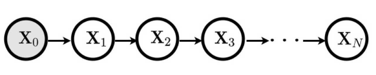
Figure 16: The PGM of a Markov chain: given the prior or initial condition $P(\mathbf{x}_{1})$, the behaviour of the system is determined by the conditional probability $P(\mathbf{x}_{t}\mid\mathbf{x}_{t-1})$

The PGM shows that the joint distribution for a sequence of observations $P(\mathbf{x}_{0},\mathbf{x}_{1},\mathbf{x}_{2},\cdots,\mathbf{x}_{N})$ can be written as the product:

$$P(\mathbf{x}_{1})P(\mathbf{x}_{2}\mid\mathbf{x}_{1})\cdots P(\mathbf{x}_{N}\mid\mathbf{x}_{N-1})=P(\mathbf{x}_{1})\prod_{t=2}^{N}P(\mathbf{x}_{t}\mid\mathbf{x}_{t-1})$$ (49)

This is also known as an observable Markov process.

A finite Markov chain is one whose range consists of a finite number of $N$ states. In this case the first probability distribution is an $N$ component vector. The transition probability $T_{\tau}(\mathbf{x}_{2}\mid\mathbf{x}_{1})$ is an $N\times N$ matrix.

Thus, the C-K equation, by using the form in Eq. 48, leads to the matrix equation

$$T_{\tau}=(T_{1})^{\tau}$$ (50)

Hence the study of finite Markov chains amounts to investigating the powers and the properties of the $N\times N$ transition matrix: this is a stochastic matrix whose elements are nonnegative and each row adds up to unity (i.e., they represent transition probabilities). One seminal application of Markov chains to scan paths has been provided by Ellis and Stark ellistark .

Case study: modelling gaze shifts as observable finite Markov chains

Ellis and Stark pioneered the use of Markov analysis for characterising scan paths ellistark in an attempt to go beyond visual inspection of the eye movement traces and application of a subjective test for similarity of such traces. In particular, they challenged the assumption of what they defined “apparent randomness”, that many studies at the time were supporting in terms of either simple random or stratified random sampling ellistark . To this end (see Fig. 17), they defined regions of interest (ROI) defined on the viewed picture, each ROI denoting a state into which the fixations can be located. By postulating that the transitions from one state to another have certain probabilities, they effectively described the generating process for these sequences of fixations as Markov processes.

t]

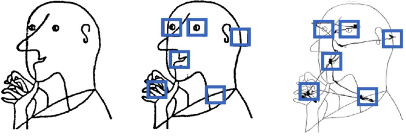
Figure 17: Markov analysis of eye movements made by a subject viewing for the first time a drawing adapted from the Swiss artist Klee (left). Centre: ROIs superimposed on the drawing, defining the states of the Markov chain: $S=\{s_{1}=\text{``left eye''},s_{2}=\text{``right eye''},s_{3}=\text{``nose''},s_{4}=\text{``mouth''},s_{5}=\text{``hand''},s_{6}=\text{``neck''}\}$. Right: saccades represented as state transitions in the state-space. Modified after hacisalihzade1992visual ; ellistark

This way, they were able to estimate the marginal probabilities of viewing a point of interest $i$, i.e., $P(X=s_{i})$, and the conditional probability of viewing a point of interest $j$ given a previous viewing of a point of interest $i$, i.e., $T(X=s_{j}\mid X=s_{i})$, where $s_{i},s_{j}$ are states in the state-space $S$ (see Fig. 17).

By comparing expected frequency of transitions according to random sampling models with observed transition frequencies, they were able to assess the statistically significant differences that occurred (subject-by-subject basis with a chi-square goodness-of-fit test on the entire distribution of observed and expected transitions). Thus, they concluded that “there is evidence that something other than stratified random sampling is taking place during the scanning” ellistark . In a further study hacisalihzade1992visual , examples have been provided for exploiting the observable Markov chain as a generative machine apt to sample simulated scan paths, once the transition matrix has been estimated / learned from data.

6.3 Levels of representation of the dynamics of a stochastic process

Up to this point, we have laid down the basis for handling eye movements in the framework of stochastic processes (cfr., Section 5 and previous subsections of the present one). Now we are ready for embracing a broader perspective.

Let us go back to Fig. 11 showing an ensemble of scan paths recorded from different observers while viewing the same image (in a similar vein, we could take into account an ensemble of scan paths recorded from the same observer in different trials). Our assumption is that such ensemble represents the outcome of a stochastic process and modelling/analysis should confront with the fundamental question: What is the probability $P(\mathbf{x},t)$ of gazing at location $\mathbf{x}$ at time $t$?

There are three different levels to represent and to deal with such question; for grasping the idea it is useful to take a physicist perspective. Consider each trajectory (scan path) as the trajectory of a particle (or a random walker). Then, Figure 11 provides a snapshot of the evolution of a many-particle system. In this view, the probability $P(\mathbf{x},t)$ can be interpreted as the density $\rho(\mathbf{x},t)$ (number of particles per unit length, area or volume) at point $\mathbf{x}$ at time $t$. In fact the density $\rho(\mathbf{x},t)$ can be recovered by multiplying the probability density $P(\mathbf{x},t)$ by the number of particles.

The finest grain of representation of a many-particle system is the individual particle, where each stochastic trajectory becomes the basic unit of the probabilistic description of the system. This is the microscopic level. In its modern form, it was first proposed by the french physicist Paul Langevin, giving rise to the notion of random walks where the single walker dynamics is governed by both regular and stochastic forces (which resulted in a new mathematical field of stochastic differential equation, briefly SDE, cfr. Box 11). At this level, $P(\mathbf{x},t)$ can be be obtained by considering the collective statistical behaviour as given by the individual simulation of many individual particles (technically a Monte Carlo simulation, see Box 4 and refer to Figure 21 for an actual example)

In the opposite way, we could straightforwardly consider, in the large scale limit, the equations governing the evolution of the space-time probability density $P(\mathbf{x},t)$ of the particles. Albert Einstein basically followed this path when he derived the diffusion equation for Brownian particles einstein1905motion . This coarse-grained representation is the macroscopic level description.

A useful analogy for visualising both levels is provided by structure formation on roads such as jam formation in freeway traffic. At the microscopic scale, one can study the motion of an individual vehicle, taking into account many peculiarities, such as motivated driver behaviour and physical constraints. On the macroscopic scale, one can directly address phase formation phenomena collectively displayed by the car ensemble.

How do we relate the macroscopic and the microscopic levels? The crucial link is provided by the intermediate mesoscopic level of description. Pushing on with the traffic analogy, instead of following the motion of each vehicle (microscopic level), a stochastic cluster (mesoscopic) of congested cars is considered by starting to average or integrating microscopic fundamental laws. Then, further coarse-graining (and related approximations) allow to reach the macroscopic description where single vehicle behaviour has no place.

In comparison with the microscopic approach based on SDEs, the mesoscopic description does not allow to get individual realisations of the process but yet keeps the whole amount of statistical information of the underlying microscopic process. Technically it consists in finding integral or integro-differential equations for the probability that governs the evolution of the system. In the picture we have so far outlined the mesoscopic level is represented by the Chapman-Kolmogorov equation. At the microscopic level we actually consider the dynamics of the particle as governed by a regular force plus a fluctuating, random force due to the incessant molecular impacts. The C-K equation coarse-grains the landscape stating that the probability of a particle being at a point $\mathbf{x}+\Delta\mathbf{x}$ at time $t+\Delta t$ is given by the probabilities of all possible “pushes” $\Delta\mathbf{x}$, multiplied by the probability of being at $\mathbf{x}$ at time $t$. This assumption is based on the independence of the “push” of any previous history of the motion; it is only necessary to know the initial position of the particle at time $t$ not at any previous time. This is the Markov postulate, and the C-K equation is the central dynamical equation for all Markov processes.

Summing up, the passage from a microscopic description to a macroscopic one, can be envisioned as a coarse-graining operation. At the mesoscopic level an appropriately chosen coarse-graining of the observation time-scale, permits the physical process to be described as Markovian, and such coarse-graining allows to switch from the individual particle to a density of particles $\rho(\mathbf{x},t)$. Subsequently, under the same coarse-graining, the C-K equation can be reduced to a master equation or a diffusion equation describing the evolution of the system at the macroscopic level. More details are given in the following subsections.

The microscopic level

The microscopic description of a system amounts to writing down the evolution equations or differential equations (see Box 10) that describe the fine-grained dynamics of individual trajectories: e.g., the path of a Brownian particle or the scan path of an eye-tracked observer. A simple form of such equations is the following:

$$\overbrace{\frac{dx}{dt}}^{\text{state-space rate of change}}=\overbrace{a(x,t)}^{\text{deterministic comp.}}+\overbrace{b(x,t)\xi(t)}^{\text{stochastic comp.}},$$ (51)

which we call the Langevin equation, in analogy with the well known equation that in statistical physics describes the time evolution of the velocity of a Brownian particle. In Eq. (51) the drift term $a(x,t)$ represents the deterministic component of the process; the diffusive component $b(x,t)\xi(t)$ is the stochastic component, $\xi(t)$ being the “noise” sampled from some probability density, i.e. $\xi(t)\sim P(\xi)$, usually a zero-mean Normal distribution.

Equation (51) is an SDE, which in a more formal way can be written in the Itô form of Eq. (65) as detailed in Box 11.

Table 10: Dynamical systems and differential equations

A system that changes with time is called a dynamical system. A dynamical system consists of a space of states and entails a law of motion between states, or a dynamical law. The deterministic component of Langevin equation (51)

$$\frac{dx(t)}{dt}=a(x(t),t)$$ (52)

is one such law, the variable $x(t)$ being the variable that, moment to moment, takes values in the state space of positions. Equation (52) is a differential equation describing the rate of change of state-space variable $x$.

In simple terms, a dynamical law is a rule that tells us the next state given the current state. This can be more readily appreciated if we recall the definition of derivative given in Box 1, but avoiding the shrinking operation ($\lim_{\Delta t\rightarrow 0}$), i.e. we approximate the derivative as a discrete difference

$$\frac{dx(t)}{dt}\approx\frac{x(t+\Delta t)-x(t)}{\Delta t}.$$

By assuming for simplicity a unit time step, i.e., $\Delta t=1$ and substituting in Eq. (52):

$$\overbrace{x(t+1)}^{\text{next state}}=\overbrace{x(t)}^{\text{current state}}+a(x(t),t)$$ (53)

Equation (53) is the discrete-time version of the differential equation (52), namely a finite-difference equation. The model in discrete time emphasises the predictive properties of the law: indeed, with the scientific method we seek to make predictions about phenomena that are subject to change. Caveat: we should always be cautious about how predictable the world is, even in classical physics. Certainly, predicting the future requires a perfect knowledge of the dynamical laws governing the world but at the same time entails the ability to know the initial conditions with almost perfect precision. However, perfect predictability is not achievable, simply because we are limited in our resolving power. There are cases in which the tiniest differences in the initial conditions (the starting state), leads to large eventual differences in outcomes. This phenomenon is called chaos.

The law formalised in Eqs. (52) or (53) are deterministic. In stark contrast, the Langevin equation (51) “corrupts” the deterministic law of motion with the “noise” introduced by the RV $\xi(t)$. Thus, the eventual outcome is not deterministic but stochastic (though it may be predictable in probability). Langevin equation is but one example of stochastic differential equation (SDE).

Concretely, the construction of a trajectory (a solution) can be performed by refining the intuitive discretisation approach presented in Box 10. Eq. (51) is discretised as in Eq. (67) by executing a sequence of drift and diffusion steps as illustrated in Fig. 19.

In continuous time a $2$-dimensional random motion of a particle, with stochastic position/state $\mathbf{x}(t)$, under the influence of an external force field siegert2001 , can be described by the Langevin stochastic equation

$$d\mathbf{x}(t)=\mathbf{A}(\mathbf{x},t)dt+{\mathbf{B}}({\mathbf{x}},t)\bm{\xi}dt.$$ (54)

As in the one-dimensional case, the trajectory of ${\mathbf{x}}$ is determined by a deterministic part $\mathbf{A}$, the drift, and a stochastic part ${\mathbf{B}}({\mathbf{x}},t)\bm{\xi}dt$, where $\bm{\xi}$ is a random vector and $\mathbf{B}$ is a diffusion factor.

By simulating from Langevin-like equations, for suitable choice of parameters $\mathbf{A}$, $\mathbf{B}$ and noise distribution $P(\bm{\xi})$ (which is likely to be non Gaussian as we will see) it is possible to obtain trajectories that are similar to the individual trajectories shown in the left panel of Fig. 18.

The mesoscopic level

t]

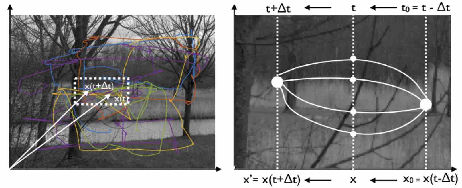
Figure 18: Left panel: the ensemble of scan paths that was presented in Fig. 11. At the microscopic level, each trajectory can be seen as the output of the simulation of Langevin equation. Right panel: a close-up of the window selected from the image in the left panel (dotted line). The mesoscopic representation used by the C-K equation for computing the conditional probability of shifting the gaze from $(\mathbf{x}_{0},t_{0})$ to $(\mathbf{x}^{\prime},t+\Delta t)$. Here the individual trajectories are replaced by the particle densities around such points. $\Delta t$ is a small time interval

If we select an appropriate spatio-temporal scale we can coarse-grain our description by summarising single particle dynamic behaviours in terms of variations on particle densities at different points, say $\mathbf{x}_{0}$ and $\mathbf{x}^{\prime}$, as illustrated in the right panel of Figure 18. This density based description to an actual image the abstract C-K construction we previously presented in Fig. 15. In this case, by considering the state $\mathbf{x}=(n,m)$ as indexing a discrete grid of image pixels and, admittedly, to avoid burdening mathematical details, we can rewrite C-K equation (43) in discrete form:

$$P(\mathbf{x}^{\prime},t+\Delta t\mid\mathbf{x}_{0},t_{0})=\sum_{\mathbf{x}}P(\mathbf{x}^{\prime},t+\Delta t\mid\mathbf{x},t)P(\mathbf{x},t\mid\mathbf{x}_{0},t_{0}).$$ (55)

Now, the microscopic individual trajectories are replaced on a coarse-grain scale by the particle densities around such points and single particle dynamics is summarised by the Markov-based transition probability $P(\mathbf{x}^{\prime},t+\Delta t\mid\mathbf{x}_{0},t_{0})$. Note that even in the discrete case where the C-K equation has an intuitive form, it is equally a complicated equation that a function of four parameters namely has to fulfil.

However, from this level it is possible to compute the evolution of particle densities in a larger scale limit, where we consider the coarse-grained dynamics of the overall pdf of the many-particle system, as detailed below.

The macroscopic level

There are two possible macroscopic limits from mesoscopic equations: the macroscopic limit in time or in space. When we consider the macroscopic limit in time of the C-K equation, we obtain the Master equation; when we consider the macroscopic limit both in time and in the state space of the C-K equation, we obtain the famous Fokker-Planck equation (F-P).

To illustrate how this works we present a simple derivation of the Master equation starting from the discrete C-K equation (55). First of all, we assume that $\Delta t$ is a small time interval. Then we characterise the short time properties of the conditional probability $P(\mathbf{x}^{\prime},t+\Delta t\mid\mathbf{x},t)$, where $\mathbf{x}$ denote a number of intermediate states between the initial state $\mathbf{x}_{0}$ and the ending state $\mathbf{x}^{\prime}$ as usually considered in the C-K construction (cfr. Fig. 18, right).

We also assume that a transition from $\mathbf{x}$ to state $\mathbf{x}^{\prime}$ is proportional to time when time gets small and that such transition occurs at a transition rate which we denote $w(\mathbf{x}^{\prime}\mid\mathbf{x})$ (density variation per unit time). Thus:

$$P(\mathbf{x}^{\prime},t+\Delta t\mid\mathbf{x},t)\approx\Delta t\times w(\mathbf{x}^{\prime}\mid\mathbf{x}),$$ (56)

which obviously holds only for $\mathbf{x}^{\prime}\neq\mathbf{x}$ since $w(\mathbf{x}\mid\mathbf{x})=0$.

However, to be complete we must also consider the probability that no state transition occurs in the small time interval:

$$Q(\mathbf{x})=1-\Delta t\sum_{\mathbf{x}^{\prime}\neq\mathbf{x}}w(\mathbf{x}^{\prime}\mid\mathbf{x}).$$ (57)

Eventually,

$$P(\mathbf{x}^{\prime},t+\Delta t\mid\mathbf{x},t)\approx\Delta t\times w(\mathbf{x}^{\prime}\mid\mathbf{x})+Q(\mathbf{x})\delta_{\mathbf{x}^{\prime},\mathbf{x}},$$ (58)

where $\delta_{\mathbf{x}^{\prime},\mathbf{x}}$ is the Kroenecker symbol: $\delta_{\mathbf{x}^{\prime},\mathbf{x}}=0$ when $\mathbf{x}^{\prime}\neq\mathbf{x}$, and $\delta_{\mathbf{x}^{\prime},\mathbf{x}}=1$ when $\mathbf{x}^{\prime}=\mathbf{x}$.

If we plug the right hand side of Eq. (58) in C-K equation (55), after some (tedious and unrelevant) algebra we obtain the following result:

$$P(\mathbf{x}^{\prime},t+\Delta t\mid\mathbf{x}_{0},t_{0})=P(\mathbf{x}^{\prime},t\mid\mathbf{x}_{0},t_{0})+$$ (59)

$$\Delta t\sum_{\mathbf{x}}\left[w(\mathbf{x}^{\prime}\mid\mathbf{x})P(\mathbf{x},t\mid\mathbf{x}_{0},t_{0})-w(\mathbf{x}\mid\mathbf{x}^{\prime})P(\mathbf{x}^{\prime},t\mid\mathbf{x}_{0},t_{0})\right].$$

Note that in the limit $\Delta t\rightarrow 0$, we can write

$$\lim_{\Delta t\to 0}\frac{P(\mathbf{x}^{\prime},t+\Delta t\mid\mathbf{x}_{0},t_{0})-P(\mathbf{x}^{\prime},t\mid\mathbf{x}_{0},t_{0})}{\Delta t}=\frac{\partial P(\mathbf{x}^{\prime},t\mid\mathbf{x}_{0},t_{0})}{\partial t}$$

This is the definition of a partial derivative of first order with respect to time, denoted by the symbol $\frac{\partial}{\partial t}$.

Using such definition in Eq. (6.3), in the limit $\Delta t\rightarrow 0$:

$$\frac{\partial P(\mathbf{x}^{\prime},t\mid\mathbf{x}_{0},t_{0})}{\partial t}=\sum_{\mathbf{x}}\left[w(\mathbf{x}^{\prime}\mid\mathbf{x})P(\mathbf{x},t\mid\mathbf{x}_{0},t_{0})-w(\mathbf{x}\mid\mathbf{x}^{\prime})P(\mathbf{x}^{\prime},t\mid\mathbf{x}_{0},t_{0})\right].$$ (60)

This equation can be further simplified by using the marginalisation rule

$$\sum_{\mathbf{x}_{0}}P(\mathbf{x}^{\prime},t\mid\mathbf{x}_{0},t_{0})P(\mathbf{x}_{0},t_{0})=P(\mathbf{x}_{0},t_{0})$$

Multiplying equation (60) by $P(\mathbf{x}_{0},t_{0})$ and summing over $\mathbf{x}_{0}$, we eventually obtain

$$\frac{\partial P(\mathbf{x}^{\prime},t)}{\partial t}=\sum_{\mathbf{x}}\left[w(\mathbf{x}^{\prime}\mid\mathbf{x})P(\mathbf{x},t)-w(\mathbf{x}\mid\mathbf{x}^{\prime})P(\mathbf{x}^{\prime},t)\right].$$ (61)

This is our final Master equation and has a very simple interpretation. The density $P(\mathbf{x}^{\prime},t)$ is the probability of the ensemble of observers (the many particle system) of being in (gazing at) state $\mathbf{x}^{\prime}$ at time $t$. How does this density change over time? The system can be in any state $\mathbf{x}\neq\mathbf{x}^{\prime}$ and move into the state $\mathbf{x}^{\prime}$. The system is in state $\mathbf{x}$ with probability $P(\mathbf{x},t)$ and from any of these states $\mathbf{x}$ it moves to the state $\mathbf{x}^{\prime}$ with probability $w(\mathbf{x}^{\prime}\mid\mathbf{x})P(\mathbf{x},t)$. But simmetrically, it could also already be in state $\mathbf{x}^{\prime}$ and move to one of the other states $\mathbf{x}$ with probability $w(\mathbf{x}\mid\mathbf{x}^{\prime})P(\mathbf{x}^{\prime},t)$.

In other terms the Master equation is a probability flux balance equation, best understood if $P(\mathbf{x}^{\prime},t)$ is interpreted as a particle density: the rate of change in that density (derivative) is the difference of what comes in and what goes out.

Technically speaking the Master equation (61) is a stochastic partial differential equation (PDE) defining the “law of motion” of the density $P(\mathbf{x}^{\prime},t)$ in probability space and it has been obtained by taking the limit in time of the C-K equation.

When we consider the macroscopic limit both in time and in the state space of the C-K equation, we obtain another PDF, namely the Fokker-Planck (F-P) equation.We omit the formal derivation because beyond the scope of this Chapter.

In the simple 1-dimensional case, the F-P equation for diffusive processes is the following:

$$\frac{\partial P(x,t)}{\partial t}=-\frac{\partial}{\partial x}[a(x,t)P(x,t)]+\frac{1}{2}\frac{\partial^{2}}{\partial x^{2}}[b(x,t)^{2}P(x,t)]$$ (62)

The symbols $\frac{\partial}{\partial x}$ and $\frac{\partial^{2}}{\partial x^{2}}=\frac{\partial}{\partial x}(\frac{\partial}{\partial x})$ denote partial derivatives with respect to space of first and second-order, respectively.

What is important to note is that there is a formal link between the microscopic description provided by the Langevin equation (cfr., the 1-dimensional case of Eq. 51) and the macroscopic description addressed by the F-P equation (62), which is established via $a(x,t)$ and $b(x,t)$. The term $a(x,t)$ represents a drift which is related to the average deviation of the process

$$a(x,t)=\lim_{\Delta t\to 0}\frac{\langle\Delta x\rangle}{\Delta t}.$$ (63)

over a small time interval $\Delta t$; the bracket operator $\langle\rangle$ denotes the average or expectation value of any function $f(X)$.. $\Delta x$ is a deviation or displacement in state-space

The term $b^{2}(x,t)$ represents a diffusion term, which is related to the mean square deviation of the process:

$$b^{2}(x,t)=\lim_{\Delta t\to 0}\frac{\langle(\Delta x)^{2}\rangle}{\Delta t}.$$ (64)

Eventually, at the macroscopic level, by knowing the evolution of $P(x,t)$ in time, one can obtain statistical “observables” as the moments, correlations, etc. These obviously lack microscopic details from the underlying stochastic process, which for some specific purposes may be important.

We will turn now to the fundamental example of the Wiener process to make clear the connections between the macroscopic and microscopic levels of description.

Table 11: Stochastic Differential Equations

The Langevin equation written in the form (51) poses some formal problems. Since $\xi(t)$ is noise it consists of a set of points that in some cases can be even uncorrelated. As a consequence $\xi(t)$ is often non-differentiable. Thus, $x(t)$ should be non-differentiable too, so that the left hand side of (51) is incoherent from this point of view. To overcome this problem, the $1-$dimensional Langevin equation is usually presented in the mathematically sound form:

$$dx(t)=a(x(t),t)dt+b(x(t),t)\xi(t)dt=a(x(t),t)dt+b(x(t),t)dW(t)$$ (65)

with $W(t)=\int_{0}^{t}\xi(t^{\prime})dt^{\prime}$, so that the integration of the stochastic component $\int b(x,t)dW(t)$ can be performed according to the rules of stochastic calculus (in the Itô or Stratonovich approach higham2001algorithmic ). Throughout this chapter we shall use with a certain liberality both forms (51) and (65) at our convenience. Thus, a stochastic quantity $x(t)$ obeys an Itô SDE written as in (65), if for all $t$ and $t_{0}$,

$$x(t)=x(t_{0})+\int_{t_{0}}^{t}a(x(t^{\prime}),t^{\prime})dt^{\prime}+\int_{t_{0}}^{t}b(x(t^{\prime}),t^{\prime})dW(t^{\prime})$$ (66)

A discretised version of the SDE can be obtained by taking a mesh of points $t_{i}$(Fig.19)

$$t_{0}<t_{1}<t_{2}<\cdots<t_{n-1}<t_{n}=t$$

and writing the equation as

$$x_{i+1}=x_{i}+a(x_{i},t_{i})\Delta t_{i}+b(x_{i},t_{i})\Delta W_{i}$$ (67)

Here, $x_{i}=x(t_{i})$ and

$$\Delta t_{i}=t_{i+1}-t_{i},$$ (68)

$$\Delta W_{i}=W(t_{i+1})-W(t_{i})\propto\sqrt{\Delta t_{i}}\xi_{i}.$$ (69)

The approximate procedure for solving the equation is to calculate $x_{i+1}$ from the knowledge of $x_{i}$ by adding a deterministic term $a(x_{i},t_{i})\Delta t_{i}$ and a stochastic term $b(x_{i},t_{i})\Delta W_{i}$, which contains the element $\Delta W_{i}$, namely the increment of the Wiener process. The solution is then formally constructed by letting the mesh size go to zero. The method of constructing a solution outlined above is called the Cauchy-Euler method, and can be used to generate simulations. By construction the time development of $x(t)$ for $t>t_{0}$ is independent of $x(t_{0})$ for $t>t_{0}$ provided $x(t_{0})$ is known. Hence, $x(t)$ is a Markov process.

For an intuitive, Matlab based, thorough introduction to SDEs see Higham higham2001algorithmic .

t]

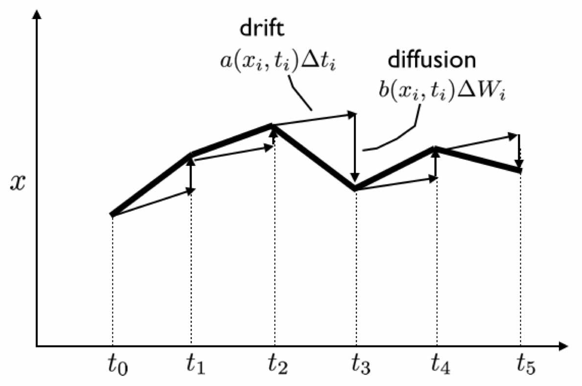
Figure 19: The Cauchy-Euler procedure for constructing an approximate solution of the Langevin SDE in the Itô form (cfr. Box 11)

Example: the Wiener process

Recall again the most famous Markov process: the Wiener process describing Brownian motion (Bm), cfr., Box 9. The SDE defining the motion of a particle undergoing 1-dimensional Brownian motion can be obtained by setting to zero the drift component $a(x,t)$ and letting $b(x,t)=\sqrt{2D}$, where $D$ is the diffusion coefficient. Thus:

$$dx=\sqrt{2D}dW(t)$$ (70)

t]

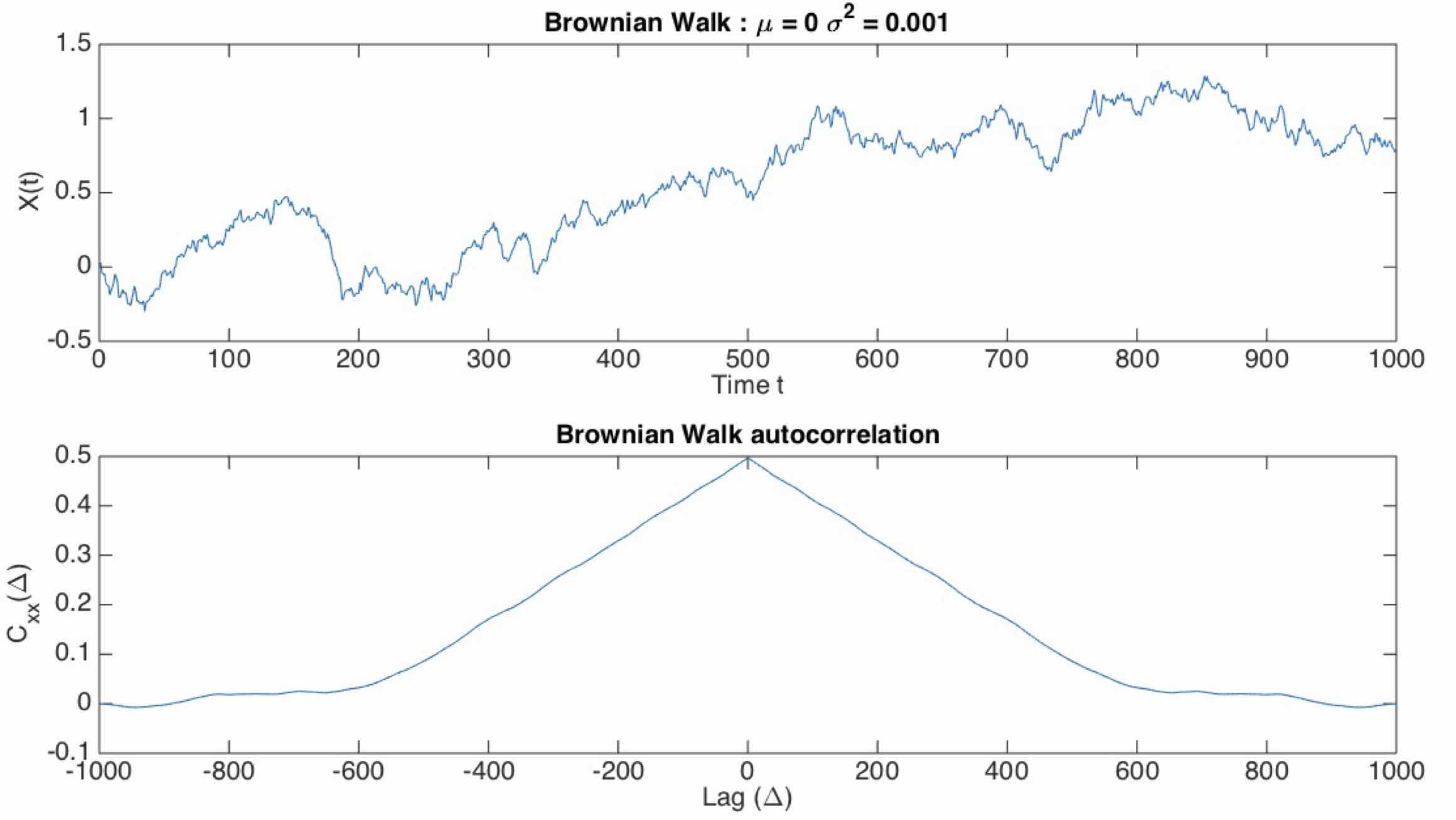
Figure 20: One dimensional Brownian motion. Top: the random walk process; bottom: the autocorrelation of the process. (cfr. Box 6)

By using Eqs. (67) and (69) introduced in Box 11, the discretised version of the Wiener process (70) over a small but finite time interval $\Delta t=T/N$, $N$ being the discrete number of integration steps, can be written as

$$x_{i+1}=x_{i}+\sqrt{2D}\Delta W_{i}=x_{i}+\sqrt{2D\Delta t_{i}}\xi_{i}$$ (71)

with $\xi$ sampled from a zero-mean Gaussian distribution of unit variance $\mathcal{N}(0,1)$

Equation 71 shows that the system describes a refined version of the simple additive random walk. Once again, it is worth noting that since the $\xi(t)$ are sampled i.i.d, then the differences in sequential observations are i.i.d, namely, $x_{i+1}-x_{i}=\Delta x_{i}$, rather than the observations themselves. In fact, if we compute the auto-correlation function of the $\{x(t)\}$ time series, it exhibits a slower decay —differently from the white noise process—, which shows how this simple random walk exhibits memory (Fig. 20).

Let us simulate the Brownian motion of a large number of particles, say $10^{5}$ particles. Resorting to a Monte Carlo approach, we can obtain this result by running in parallel $10^{5}$ random walks, each walk being obtained by iterating Eq.(71). Fig. 21 (top) shows an example of $20$ such trajectories. In probabilistic terms each trajectory is a realisation, a sample of the stochastic process $\{X(t)\}$.

We may be interested in gaining some statistical insight of the collective behaviour of all such random walkers. This can be obtained by considering the the dynamics of the pdf $P(x,t)$ describing the probability of finding a particle at position $x$ at time $t$. Empirically, we can estimate $P(x,t)$ at any time $t$ by computing the density of particles occurring within a certain bin $(x-\delta,x+\delta)$ centred on $x$, that is by computing the histogram $h(x,t)$ and normalising it with respect to the total number of particles. This procedure is shown in the bottom of Fig. 21: the empirical pdf has a nice bell shape, i.e. it is a Normal distribution, which spreads as time increases.

t]

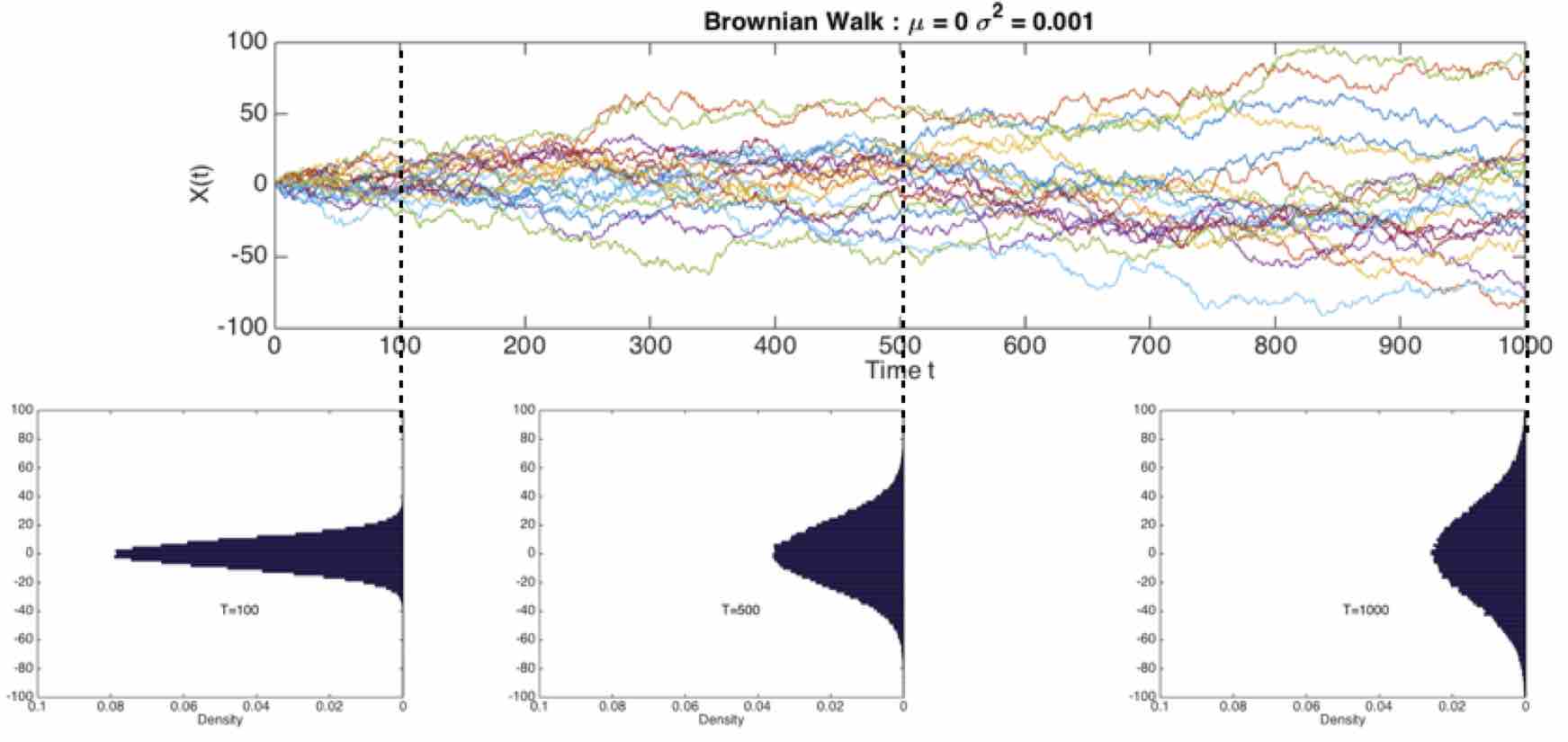
Figure 21: A Monte Carlo simulation (cfr. Box 4) of the macroscopic dynamics of $P(x,t)$ in the case of Brownian motion. Top: The simulation of individual trajectories of $10^{5}$ random walkers: only $20$ are shown for visualisation purposes. Bottom: The distributions (histograms) of the walkers, after $T=100$, $T=500$ and $T=1000$ time steps. The distribution initially concentrated at a point takes later the Gaussian form, whose width grows in time as $t^{1/2}$. This kind of diffusion is called the normal diffusion.

This insight can be given a formal justification by resorting to the macroscopic level of description of process dynamics as provided by F-P equation (62). By setting again $a(x,t)=0$ and $b(x,t)=\sqrt{2D}$:

$$\frac{\partial P(x,t)}{\partial t}=D\frac{\partial^{2}P(x,t)}{\partial x^{2}}$$ (72)

This is the well-known heat or diffusion equation. Thus, the pdf $P(x,t)$ of finding a particle at position $x$ at time $t$ evolves in time according to the diffusion equation when the underlying microscopic dynamics is such that the particle position corresponds to a Wiener process.

The solution to the heat equation (72) is the time-dependent Gaussian pdf, as anticipated in Box 9:

$$P(x,t)=\frac{1}{\sqrt{4\pi Dt}}\exp\left(-\frac{x^{2}}{4Dt}\right),$$ (73)

By comparing the Gaussian pdf variance $\sigma^{2}=4Dt$ to the definition of $b^{2}(x,t)$ given in Eq. (64), we can set the following correspondences:

$$\sigma^{2}=2Dt=b^{2}t\approx\langle x^{2}\rangle$$ (74)

In other terms for Bm, the average square deviation of the walk, and thus the spread of the Gaussian, grows linearly with time, as it can be intuitively appreciated from Fig. 21.

More precisely, define the Mean Square Displacement (MSD) of a walk that starts at position $x_{0}$ at time $t_{0}$:

$$MSD=\langle|x-x_{0}|^{2}\rangle,$$ (75)

which is, quoting Einstein, the square of the displacement in the direction of the $x$-axis “that a particle experiences on the average” EinsteinBrown . Here $x_{0}$ denotes the initial position. In the case of Brownian motion, Einstein EinsteinBrown was the first to show that:

$$MSD=2Dt$$ (76)

Note that $\langle|x-x_{0}|^{2}\rangle=\langle x^{2}\rangle+x_{0}^{2}-2x_{0}\langle x\rangle$. Hence, when the initial position is at $x_{0}=0$, $MSD=\langle x^{2}\rangle\propto t$.

Equation (76) is sometimes more generally written in terms of the Hurst exponent $H$

$$MSD=kt^{2H}$$ (77)

with $H=\frac{1}{2}$ for Bm. This is useful for characterising different kinds of diffusions, like hyperdiffusion or subdiffusion, as discussed in Box 12.

Table 12: The Hurst exponent: the Swiss army knife of diffusion processes (without SDE pain)

The Hurst exponent, $H$, is related to the signal correlation behaviour and it allows the detection of the long-range dependences. In general, properties of Gaussian diffusion may be expressed in terms of the MSD of $x$ and its relation to time:

$$MSD=\langle|x(t)-x(0)|^{2}\rangle=kt^{2H}$$ (78)

When $H=0.5$, MSD is linear in time:

$$MSD=kt,$$ (79)

which exemplifies the ordinary condition of Bm, the derivative of Bm being additive white Gaussian noise. When $H>0.5$, increments are positively correlated, i.e. the random walk shows the tendency to continue to move in the current direction. This behaviour is called persistence. In this case, MSD increases nonlinearly with respect to time, indicative of hyperdiffusion. In particular, for $H=1$,

$$MSD=kt^{2}.$$ (80)

In this case diffusion follows correlated fractional Brownian motion (fBm), whose derivative is fractional Gaussian noise.

In the case $H<0.5$, the random walk generates negatively correlated increments and is anti-persistent.

It is important to note that for $H\neq 0.5$, the increments are not independent, thus the fBm is a Gaussian process but it is not a Markov process.

Interesting work has been reported in the recent literature on the use of the $H$ exponent to analyse eye movements, e.g. by Engbert and colleagues on random walk analysis of fixational eye movements engbert2006microsaccades . For such purposes the scaling exponent $H$ can be estimated as follows engbert2006microsaccades . Consider a time series of gaze positions of length $N$, $\mathbf{x}_{1},\cdots,\mathbf{x}_{N}$. Define the displacement estimator

$$\overline{\delta^{2}(\Delta_{m})}=\frac{1}{N-m}\sum_{i=1}^{N-m}\|\mathbf{x}_{i+m}-\mathbf{x}_{i}\|^{2},$$ (81)

namely the time averaged MSD. By recalling that $MSD\approx t^{2H}$, the Hurst exponent $H$ can be obtained by calculating the slope in the plot of $\log\overline{\delta^{2}(\Delta_{m})}$ as a function of $\log\Delta_{m}$, where $\Delta_{m}=mT_{0}$ is the time lag, $T_{0}$ (ms) being the sampling time interval and $m=1,2,3,\cdots$.

More recently, Engbert has proposed more sophisticated estimation framework based on the Bayesian approach engbert2012bayesianHurst .

A last, but important remark: the equivalence

$$\overline{\delta^{2}(\Delta)}\approx\langle x(\Delta)^{2}\rangle$$ (82)

holds when the process is ergodic, where ensemble averages and long-time averages are equivalent in the limit of long measurement times.

Case study: from random walks to saccade latency

A saccade represents the output of a decision, a choice of where to look, and reaction time, or latency, can be regarded as an experimental “window” into decision processes. Typical latencies are around $200$ms (see Fig. 22(a)) whereas the sensorimotor components of a saccade are only around $60$ms: this suggests that reaction time is composed of more than the simple sum of times of for sensory input and motor output, and such extra time (also called neural procrastination) reflects the time taken for the brain to choose a response. Put simply, reaction time is a useful indicator of decision time. In experimental paradigms, reaction time varies stochastically between one trial and the next, despite standardized experimental conditions. Furthermore, distribution of reaction times is typically skewed, with a tail towards long reaction times (Fig. 22(a)). However, if we take the reciprocal of the latencies and plot these in a similar fashion, the resulting distribution appears Gaussian (Fig. 22(b)).

t]

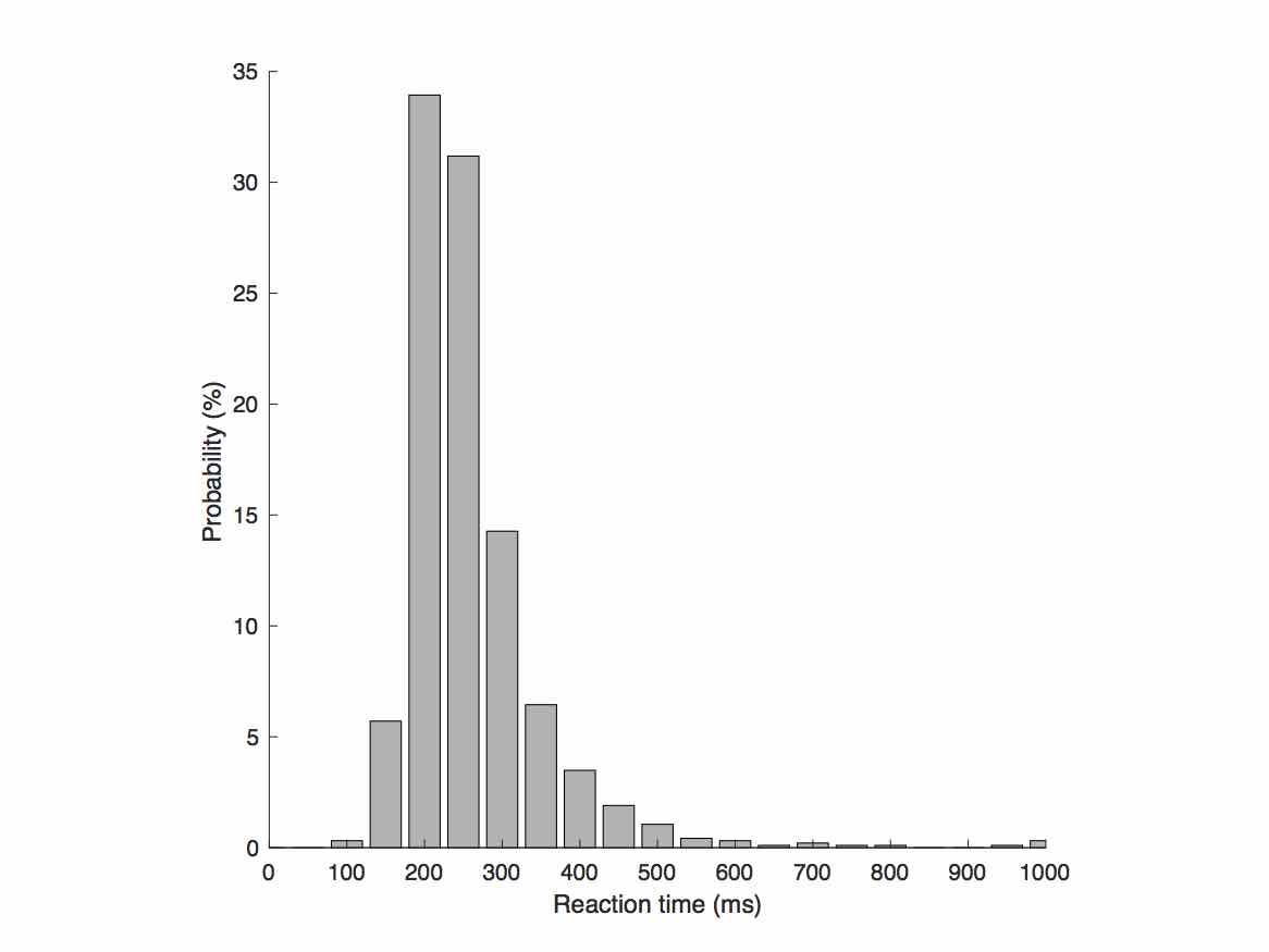
(a) Latencies

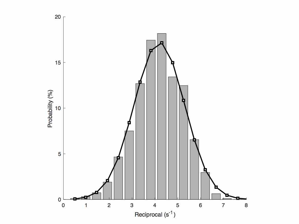
(b) Reciprocals

Figure 22: Empirical distributions (histograms) of latencies (left panel) and reciprocals (right panel). The latencies/reaction times themselves are typically skewed, with a tail towards long reaction times. When plotted as a function of reciprocal reaction time (inverse of the reaction times or promptness), the distribution looses its skewness, and it turns out to obey the most fundamental of all stochastic laws, the normal or Gaussian distribution. The reciprocal histogram can thus be approximated by a normal distribution (the black line superimposed to the histogram, with the same mean and standard deviation of actual reciprocals)carpenter1995neural ; Noorani2016

Table 13: The probit function

When confronting with reaction times and in particular with the well known Carpenter’s LATER model carpenter1995neural ; Noorani2016 , one tipically has to deal with reciprobit plots, a tool that sometimes students find difficult to conceptualise. Indeed, the subtle probit function lies behind such graphs.

Recall from your elementary probability and statistics class that a quantile function returns the value $x$ such that $F_{X}(x)=P(X\leq x)=p$ where $0<p<1$ is a probability value and $F_{X}(\cdot)$ is the cumulative distribution function (CDF) of random variable $X$. In simple words, it returns a threshold value $x$ below which random draws from the given CDF would fall $p$ percent of the time.

The probit function $probit(\cdot)$ is exactly the quantile function associated with the standardised normal distribution $\mathcal{N}(0,1)$ and the standard CDF $\Phi(\cdot)$, formally

$$probit(p)=\Phi^{-1}(p).$$ (83)

where $\Phi^{-1}(\cdot)$ is the inverse CDF of the standard normal. Clearly, by the above definition, the following properties hold:

$$\Phi(probit(p))=\Phi(\Phi^{-1}(p))=p$$

and

$$probit(\Phi(z))=\Phi^{-1}(\Phi(z))=z$$

where $z\sim\mathcal{N}(0,1)$ is a standardised random variable (the famous “z-score”) sampled from the standard normal.

Unfortunately, the standard CDF $\Phi$ and its inverse $\Phi^{-1}$ are not available in closed form, and computation requires careful use of numerical procedures (unless we do not exploit good old tables). To such end, $\Phi(z)=\frac{1}{\sqrt{2\pi}}\int_{-\infty}^{z}e^{\frac{-t^{2}}{2}}dt$ is related to the error function $erf(x)=\frac{1}{\sqrt{\pi}}\int_{-x}^{x}e^{-t^{2}}dt$ as $\Phi(z)=\frac{1}{2}\left[1+erf\left(\frac{z}{\sqrt{2}}\right)\right]$. However, we need not worry too much about these mathematical details since numerical calculations of the error and the inverse error functions are widely available in software for statistics and probability modelling.

Eventually, given a probability value $\Phi(z)=p$ from the normal CDF, the probit of such value can be computed in terms of the inverse error function $erf^{-1}(\cdot)$ as

$$probit(p)=\sqrt{2}erf^{-1}(2p-1),$$ (84)

which, for instance, in Matlab code boils down to the simple statement

prob_p = sqrt(2) * erfinv(2 * p -1)

This is all we need for producing beautiful reciprobit plots (see Fig. 23(b)).

Histograms, however, are in some sense problematic since their shape depends on the bin size and they have an effectively arbitrary vertical scale. As an alternative, cumulative histograms or empirical Cumulative Distribution Function (ECDF) are normalized (running from $0$ to $1$ or $100\%$), can represent all data without binning (continuous), thus facilitating comparisons between data sets. The ECDF $\widetilde{F_{N}}(x)$, is an unbiased estimator of the CDF, the Cumulative Distribution Function $F_{X}(x)$, of a RV $X$ (cfr. Box 13 for refreshing these basic concepts). In practice, given $N$ data points $x_{i},i=1,\cdots,N$ the computation of $\widetilde{F_{N}}(x)$ boils down to two steps: (1) count the number of data less than or equal to $x$; divide the number found in (1) by the total number of data in the sample. The ECDF of inverse reaction times previously presented in Fig. 22 is illustrated in Fig. 23(a).

An even better result can be achieved by using a non-linear probit scale (an inverse error function transformation, see Box 13, Eq. 84) for the vertical frequency axis, rather than a linear scale carpenter1995neural ; Noorani2016 . Such transformation stretches the ends of the ordinate axis in such a way as to generate a straight line if the data is indeed Gaussian, as it can be seen in Fig. 23(b). Since the latency uses a reciprocal scale, this is known as a reciprobit plot (because it combines a reciprocal and a probit scale). Such plot provides at a glance the visual impression of the two parameters describing the normal distribution of reciprocals, the mean $\mu_{r}$ and the variance $\sigma^{2}_{r}$: $\mu_{r}$ corresponds to the median of the plot (where the line intersects $p=50\%$), and the standard deviation $\sigma_{r}$ to its slope (a steep line has a small variance, a shallow one a greater one).

t]

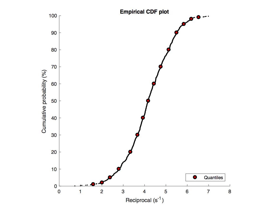
(a) Reciprocal ECDF

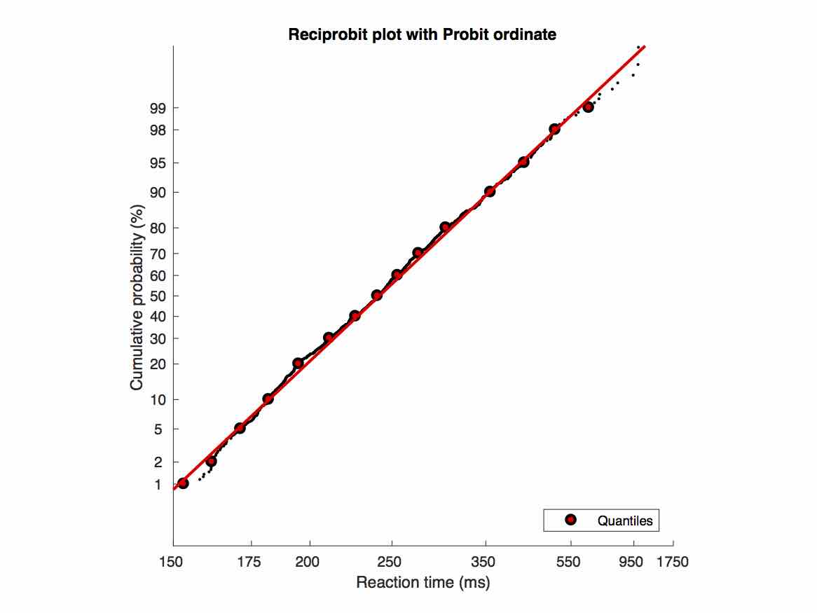
(b) Reciprobit plot

Figure 23: Empirical CDF of reciprocals (left panel) and reciprobit plot (right panel) of the same data presented in Fig. 22. In the cumulative probability of inverse reaction time, every dot is an actual individual data point, while red markers indicate quantiles at probabilities $p=0.01,0.02,0.05,0.1,0.2,0.3,\cdots,0.7,0.8,0.9,0.95,0.98,0.99$. In the right panel, the same data as in the left panel plotted as a cumulative histogram but using a probit scale. Note that the latency uses a reciprocal scale resulting in a reciprobit graph

The basic idea that reciprocal latencies follow a Gaussian or normal distribution and that these reciprocals have equal variability around a mean value $\mu_{r}$, as captured by the representations we have introduced above, lies at the heart of the LATER model. The LATER model (“Linear Approach to Threshold with Ergodic Rate” (carpenter1995neural , but see Noorani2016 for a recent review) is one of the simplest, and yet one of the most elegant and powerful models of reaction time distributions in decision tasks: it is assumed that some decision signal is accumulated over time at a constant rate of rise $r$ until a threshold is reached, at which point a response is triggered (Fig. 24, left panel). Crucially, the rate $r$ at which such decision signal accumulates is normally distributed across trials. In mathematical terms, the model is easily specified. If

1. the response is triggered when the evidence - starting from a resting level $S_{0}$ - reaches a threshold level $S_{T}$, and

2. evidence accumulates at a constant rate $r$ which, across trials, follows a normal distribution, $\mathcal{N}(\mu_{r},\sigma_{r}^{2})$,

then the response latency $T$ is determined by:

$$T=\frac{S_{T}-S_{0}}{r}.$$ (85)

If one further assumes that both $S_{0}$ and $S_{T}$ are relatively constant across trials, then the distribution of the times is the reciprocal of a normal distribution:

$$\frac{1}{T}=\mathcal{N}\left(\frac{\mu_{r}}{S_{T}-S_{0}},\left(\frac{\sigma_{r}}{S_{T}-S_{0}}\right)^{2}\right),$$ (86)

which Carpenter terms the Recinormal distribution  carpenter1995neural ; Noorani2016 .

t]

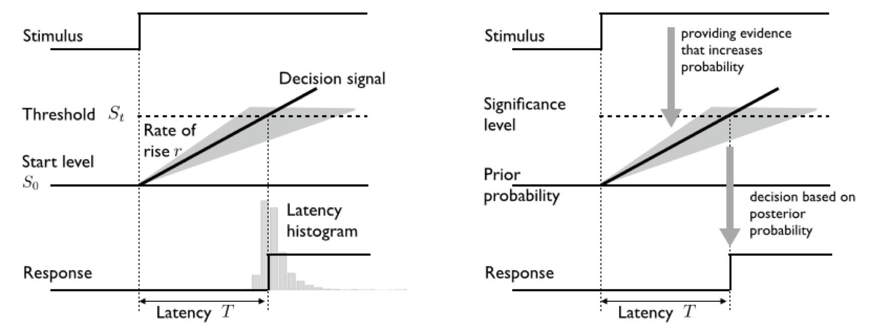
Figure 24: The LATER model carpenter1995neural . Left: the essential model. Right: LATER as an ideal Bayesian decision-maker (see Box , for a formal discussion)

The stochasticity behind the LATER model can be described at the macroscopic level, in terms of full probability distribution functions, by interpreting LATER as an optimal model of Bayesian decision making, see Box 14 and Fig. 24 (right).

The corresponding description at the microscopic level explains the LATER model in terms of a random walk model. In this perspective, we consider the function $S(t)$, as the evidence accumulated at time $t$ starting from prior level $S(0)=S_{0}$ in the process of reaching the threshold $S_{T}$. The random “trajectory” in time of $S(t)$ is that of a drifting gaussian random walker as shown in Fig. 25. Indeed, it can be formally shown that the average accumulation of evidence $<S(t)>$ with mean rate $r$ is described by a normal distribution centred at a mean $S_{0}+rt$ having variance at time $t$ equal to $\sigma_{r}^{2}t^{2}$ moscoso2008theory . Then the microscopic behaviour of the random walker $S(t)$ is described by a Langevin-type SDE of drift $r$ and diffusion coefficient $\sigma_{r}\sqrt{2t}$:

$$dS(t)=rdt+\sigma_{r}\sqrt{2t}dW(t),$$ (87)

where $W(t)$ is the standard Wiener process with linear drift. Thus LATER can be considered a non-linear version of the Drift Diffusion Model ratcliff2008 of decision making. Note how the random walk model provides the microscopic dynamics of how the long-tail skewed distribution of reaction times is originated (Fig. 25).

t]

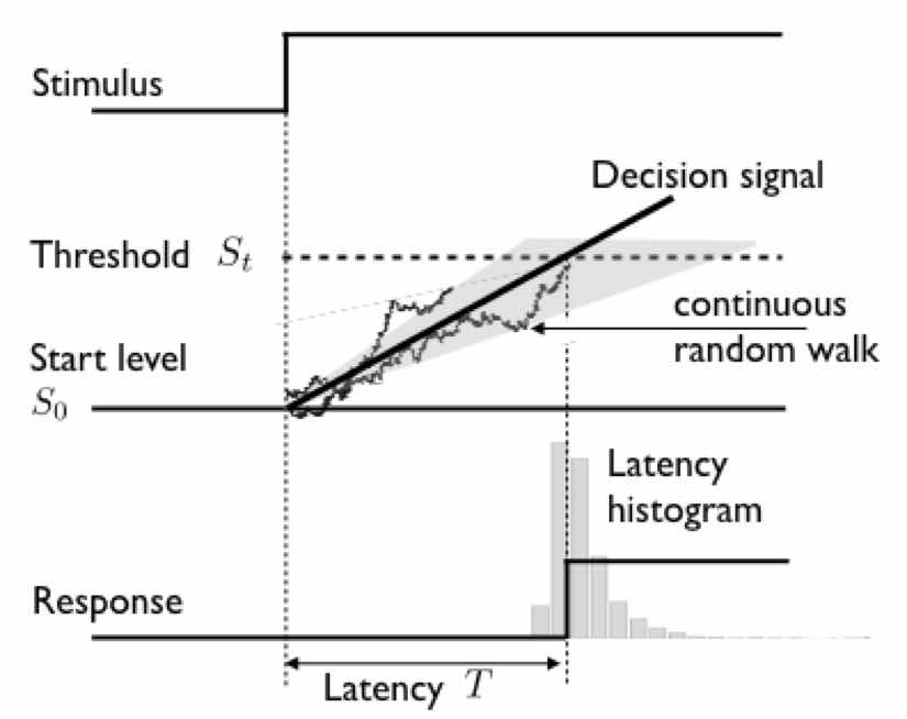
Figure 25: The LATER model as a diffusion model of decision making based on continuous random walks generated through the Langevin-type SDE of Eq. 87. Two trajectories only are shown for graphical clarity.

One general implication of all this is that the large random variation observed in latencies is not the result of noise at the input, as has commonly been supposed, but represents a gratuitous, “deliberate” randomising device (summarised by the random term $dW(t)$ in Eq. 87). It has been surmised that its purpose is to prevent the generation of undesirably stereotyped behaviour - a roulette-wheel within the brain, that one may or may not care to think of as the basis for the sense of free will and creativity Noorani2016 .

Eventually, it is worth pointing out that the predictions of latencies from random walk models and from the original LATER model are very similar, and in fact can only really be distinguished when there are a vast number of data points for latencies.

Table 14: LATER as a Bayesian decision-maker

Classic, frequentistic hypothesis testing considers the likelihood ratio $\frac{P(\mathcal{D}\mid\mathcal{H})}{1-P(\mathcal{D}\mid\mathcal{H})}$, where $P(\mathcal{D}\mid\mathcal{H})$ is the likelihood of the hypothesis $\mathcal{H}$ being tested, e.g., $\mathcal{H}=\textsf{``the stimulus is present''}$, and $\mathcal{D}$ is the evidence provided by the stimulus. In Bayesian hypothesis testing, posterior and prior probabilities need to be taken into account. Denote $P(\mathcal{H})$ the prior probability of the hypothesis $\mathcal{H}$ and $P(\mathcal{H}\mid\mathcal{D})$ the posterior probability of the hypothesis given the evidence $\mathcal{D}$.

At the macroscopic description level, LATER can be directly interpreted as an optimal Bayesian model of hypothesis testing as sketched in the right panel of Fig. 24.

To such end, simply rewrite Eq. (85) as

$$S(T)=S(0)+rT$$ (88)

Then, by using Bayes’ rule, we can rewrite the LATER parameters in Eq. (88) in terms of log-odds (namely, the log-ratio of the probability that an event will happen to the probability that the event will not happen):

$$S(T)=\log\frac{P(\mathcal{H}\mid\mathcal{D})}{1-P(\mathcal{H}\mid\mathcal{D})}=\overbrace{\log\frac{P(\mathcal{H})}{1-P(\mathcal{H})}}^{S(0)}+\int_{0}^{T}\overbrace{\log\frac{P(\mathcal{D}\mid\mathcal{H})}{1-P(\mathcal{D}\mid\mathcal{H})}}^{r}dt=S(0)+rT,$$ (89)

where the starting level $S(0)$ denotes the log-prior odds $\log\frac{P(\mathcal{H})}{1-P(\mathcal{H})}$ and the rate of information intake $r$ is the log Bayes factor of the stimulus.

Thus, the accumulated evidence $S(T)$ is an optimal estimate of the log-posterior odds $\log\frac{P(\mathcal{H}\mid\mathcal{D})}{1-P(\mathcal{H}\mid\mathcal{D})}$ (a.k.a., the logit of the posterior probability) of the hypothesis being tested

6.4 Walking on the safe side: the Central Limit Theorem

Once more, consider Eq. (71), namely the discretised version of the Wiener process. We rewrite here - with step index $n=i+1$ - for the reader’s convenience:

$$x_{n}=x_{n-1}+\sqrt{2D}\Delta W_{n-1}.$$ (90)

It is easy to see that by repeated substitution and by assuming the initial condition $x_{0}=0$, after $n$ integration steps:

$$\begin{split}x_{n}&=x_{n-1}+\sqrt{2D}\Delta W_{n-1}\\ &=x_{n-2}+\sqrt{2D}\Delta W_{n-2}+\sqrt{2D}\Delta W_{n-1}\\ &=x_{n-3}+\sqrt{2D}\Delta W_{n-3}+\sqrt{2D}\Delta W_{n-2}+\sqrt{2D}\Delta W_{n-1}\\ &=\cdots\\ &=\sum_{i=0}^{n-1}\sqrt{2D}\Delta W_{i}\end{split}$$ (91)

Note that by definition of Brownian motion, the Wiener increment $\Delta W_{i}$ is zero-mean Gaussian distributed with variance $\sigma^{2}=\Delta t_{i}$, that is $\Delta W_{i}\sim\mathcal{N}(0,\Delta t_{i})$. By using elementary properties of Gaussian RVs, the increment $\Delta W_{i}$ can be computed by i) sampling $\xi_{i}\sim\mathcal{N}(0,1)$ and ii) multiplying $\xi_{i}$ by the standard deviation $\sigma=\sqrt{\Delta t_{i}}$, namely:

$$\Delta W_{i}=\sqrt{\Delta t_{i}}\xi_{i}.$$

Then, Eq. (91) can be simply written as

$$x_{n}=\sum_{i=0}^{n-1}\sqrt{2D\Delta t_{i}}\xi_{i}.$$ (92)

This result is nothing but the answer to our fundamental question, “What is the probability $P(x_{n})$ of being at point $x_{n}$ after $n$ steps?” As before, the final position $x_{n}$ is a zero-mean Gaussian random variable with variance $\sigma^{2}=2Dt_{n}$ (assuming initial time $t_{0}=0$). Thus, $P(x_{n})=\mathcal{N}(0,2Dt_{n})$.

In short, by exploiting the simple property that the sum of independent Gaussian RVs (here the particle displacements) is a Gaussian RV, we have derived (in discrete form) the result discussed in Box 9: the probability $P(\mathbf{x},t)$ of a Brownian particle being at location $\mathbf{x}$ at time $t$ is a Gaussian distribution $\mathcal{N}(0,2Dt)$. Indeed, the Monte Carlo simulation presented in Figure 21, which illustrates both the microscopic trajectories of a large number of Brownian particles and the macroscopic evolution of the solution of the diffusion equation, is a procedure based on Eq. (92): 1) find the cumulative sums up to $x_{n}$ for a large number of walkers, and 2) compute their histogram to approximate $P(\mathbf{x},t)$.

Though intuitive, this view is an overly simplified picture of the whole story. To see why, consider a very simple kind of discrete random walker, an instantiation of the basic model presented at the very beginning in Box 7, Eq. (31).

At fixed time intervals $\Delta t$ the walker either jumps to the right with probability $p$ or to the left with probability $q=1-p$. The intuition is that for $p=\frac{1}{2}$, at each step the walker is tossing a fair coin to make the left/right decision.

The microscopic behaviour of the walker is governed by the following discrete equation:

$$x_{n}=x_{n-1}+(2\xi_{n}-1),\textsf{ }n=1,2,\cdots,$$ (93)

where $x_{0}$ is the initial position, e.g. $x_{0}=0$. The discrete RV $\xi_{n}\in\{0,1\}$ stands for the coin toss at step $n$, and it is sampled from the Bernoulli distribution, namely $\xi_{n}\sim Bern(p)=p^{\xi_{n}}q^{1-\xi_{n}}$. In other terms $\{\xi_{n}\}_{n\geq 1}$ is a Bernoulli process.

The dynamics behind Eq. (93) is simple: at each step, if $\xi_{n}=0$, then Eq.(93) gives $x_{n}=x_{n-1}+1$ (right step); otherwise, $x_{n}=x_{n-1}-1$ (left step). Figure 26(a) shows five trajectories of the simple walker drawn by iterating Eq. (93) $2000$ steps. For such a long sequence, trajectories look similar to those produced by a Gaussian random walker (Brownian particle). This becomes evident by inspecting the macroscopic behaviour as illustrated in Figure 26(b). The collective behaviour of $1000$ walkers at a step $n$ is obtained by computing for each walker the sum of a number of i.i.d displacements/increments up to step $n$, as in Eq. (92), then the (empirical) distribution $P(x_{n})$ is computed. The figure shows two “snapshots” of the evolution of $P(x_{n})$ at $n=500$ and $n=2000$: it is easy to see that its behaviour is that of a Gaussian distribution spreading in time, much like the Brownian diffusion behaviour shown in Figure 21. To better visualise such trend, we also plot the Gaussian distributions fitted at the same time steps.

t] .

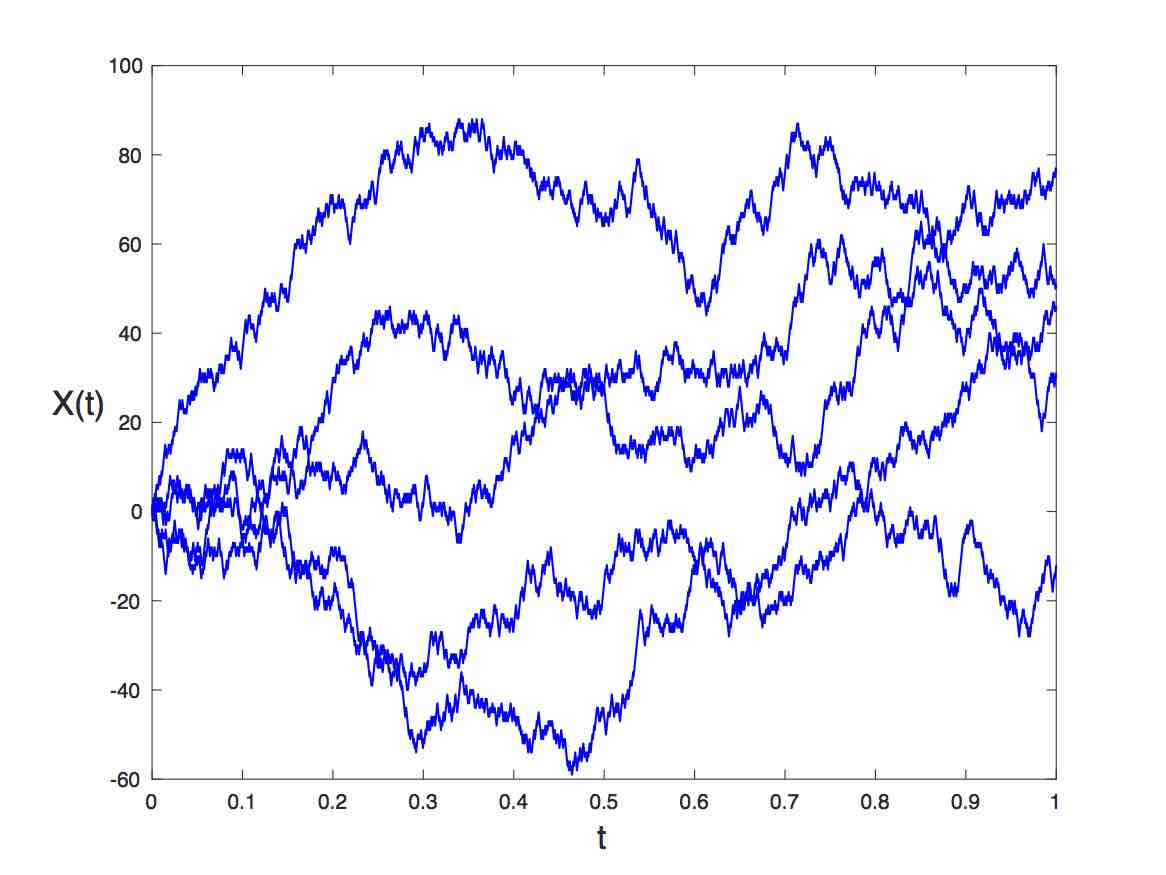
(a) Microscopic behaviour

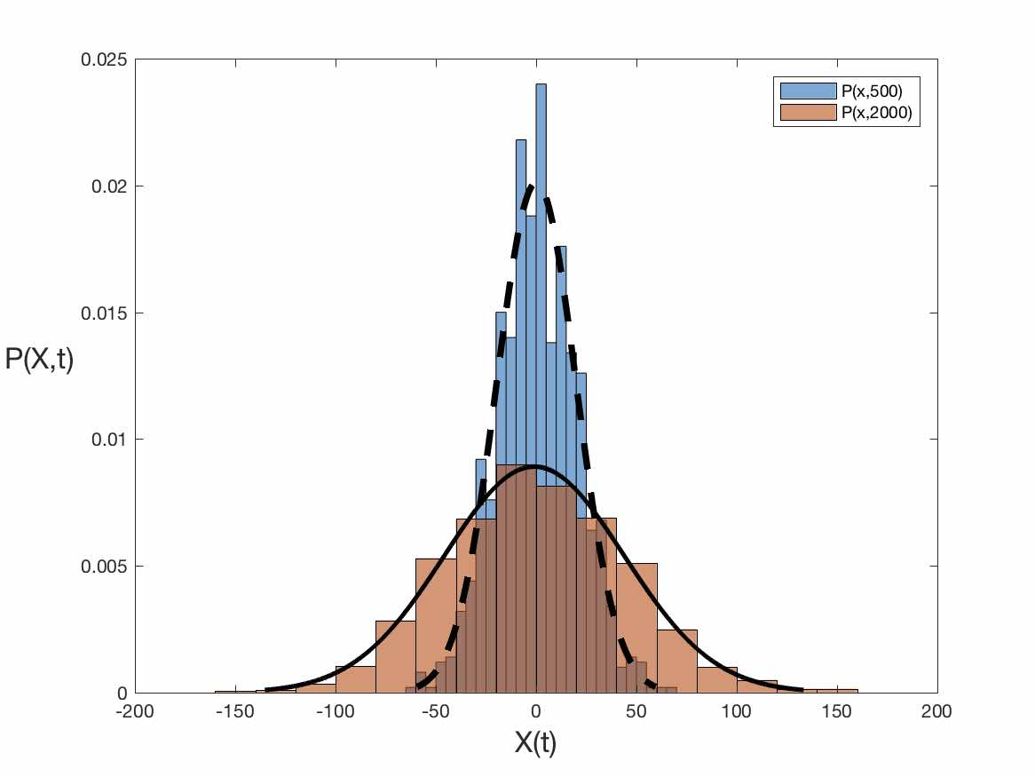
(b) Macroscopic behaviour

Figure 26: Microscopic and macroscopic behaviour of the simple random walker. Panel 26(a) shows five among $1000$ trajectories simulated via Eq. (93), for $2000$ iteration steps. Panel 26(b): the macroscopic behaviour of the many-walker system captured by computing the empirical distributions $P(x_{n})$ at steps $n=500$ and $n=2000$. Both distributions are overlaid with the Gaussian pdfs fitted at the same time steps (dotted and continuous line, respectively)

This result is not surprising: the Gaussian or Normal distribution correctly describes an amazing variety of phenomena. Most important for our purposes, the bell-shaped curve appears in nature ubiquitously due to the wide applicability of the Central Limit Theorem (CLT).

The key idea behind the classical CLT (but see Box 15 for more details) is the following. If we sum a large number $n$ of RVs $X_{i}$ that are

1. statistically independent and

2. identically distributed (i.i.d), and that

3. have a finite variance,

the distribution $P(S_{n})$ for the sum $S_{n}=\sum_{i=1}^{n}X_{i}$ converges to a Gaussian distribution with mean $n\mu$ and variance $n\sigma^{2}$, namely, $P(S_{n})\approx\mathcal{N}(n\mu,n\sigma^{2})$.

The CLT theorem generalises the thorough intuition we initially gained by exploiting the Gaussian nature of a Brownian random walk. If a trajectory consists of a set of independent displacements with finite variance, then the total distance covered (the sum of these displacements) follows a Gaussian law whose variance is proportional to the number of these displacements (and, in consequence, proportional to time).

If the three conditions required by the CLT are fulfilled, then the MSD will behave at large times like $\langle x(t)^{2}\rangle\propto t$ (no matter how complicated the motion pattern is) in the limit $t\to\infty$. Such scaling law $\langle x(t)^{2}\rangle\propto t$, as previously stated, is characteristic of the diffusion equation, but it also arises asymptotically in many other cases. This is not a coincidence but a direct consequence of the baseline CLT.

A tenet of this Chapter, following Paul and Baschnagel paul2013stochastic , is exploiting the classical CLT as the pivotal concept to distinguish stochastic behaviours that occur within its limits and behaviours that violate its limits. Examples of the latter are considered in the following Section.

Table 15: The Gaussian bell tolls for thee: The Central Limit Theorem

In a nutshell, the simplest form of the CLT states that if one sums together many independent and identically distributed (i.i.d) random variables with finite variance, then the probability density of the sum will be close to a Gaussian.

Formally, consider $n$ i.i.d RVs $X_{1},X_{2},\cdots,X_{n}$, with mean

$$\langle X_{i}\rangle=\mu$$

and finite variance

$$Var(X_{i})=\sigma^{2}<\infty$$

for all $i=1,\cdots,n$. Consider then the RV $S_{n}$, which is the sum

$$S_{n}=X_{1}+X_{2}+\cdots+X_{n}.$$ (94)

Then, as $n\to\infty$, the distribution of the normalised sum $\frac{S_{n}-n\mu}{\sigma\sqrt{n}}$ converges to the standard Gaussian distribution. More precisely, for $-\infty<a<\infty$

$$\lim_{n\to\infty}P\left(\frac{S_{n}-n\mu}{\sigma\sqrt{n}}\leq a\right)=\frac{1}{\sqrt{2\pi}}\int_{-\infty}^{a}e^{-\frac{x^{2}}{2}}dx,$$ (95)

where $\frac{1}{\sqrt{2\pi}}e^{-\frac{x^{2}}{2}}=\mathcal{N}(0,1)$ is the standard Normal PDF with zero mean and unit variance.

The two most common manifestations of the CLT are the following. First, as $n\to\infty$, the sum $S_{n}$ “tends” to a Gaussian variable with distribution $\mathcal{N}(n\mu,n\sigma^{2})$. Second, the same holds for $\frac{S_{n}}{n}$, where

$$\frac{S_{n}}{n}=\frac{X_{1}+X_{2}+\cdots+X_{n}}{n}=\frac{1}{n}\sum_{i=1}^{n}X_{i},$$

which is nothing but the empirical mean or sample average. Namely, $\frac{S_{n}}{n}$ “tends” to the distribution $\mathcal{N}\left(\mu,\frac{\sigma^{2}}{n}\right)$.

If these issues might seem too abstract or of limited interest for you, recall that you have been trained in your daily lab work to collect results from several repeated measurements, to take mean values and to eventually estimate confidence intervals by using tables from the Gaussian distribution. Your data do not necessarily follow a Gaussian distribution, yet you are not worried about. Any problem where the final output results from the average over a set of identical and independent variables with finite variance leads to a Gaussian PDF. More often than not, the CLT is your unconscious safety belt.

This is the “baseline” or classical CLT (a.k.a. the Lindeberg-Lévy CLT). However, it is worth mentioning that the CLT comes in various stronger and weaker forms schuster2016stochasticity . Under certain conditions, the RVs $X_{i}$ are not required to be identically distributed. In such case we have different variances, $Var(X_{i})=\sigma_{i}^{2}$ but the CLT still holds if the contribution of any individual random variable to the overall variance $\sigma_{n}^{2}=\sum_{i=1}^{n}\sigma_{i}^{2}$ is arbitrarily small for $n\to\infty$ (Lindeberg’s condition).

What happens if the $X_{i}$ are originated from a distribution whose variance is not finite? It is indeed the case that there are experimental time series (e.g., saccades in free viewing, go back to Fig. (4)), for which the distribution of independent increments exhibit much fatter tails than the normal, and sometimes considerable skewness as well. In Figure 8 we have seen one such example: the Cauchy distribution with a power-law tail (see Box 16). The Cauchy distribution does not have a finite variance. The Generalized CLT - due to Gnedenko, Kolmogorov and Lévy - states that the sum of a number of RV with a power-law tail will tend to a non Gaussian $\alpha$-stable distribution (stable Lévy noise) as $n\to\infty$ paul1954theorie ; kolmogorov1954limit . We will see in Section 7.2, that such kind of heavy-tailed distributions play an important role in the modelling of saccadic eye movements.

7 Walking on the wild side: eye movements beyond the CLT

In spite of the nice behaviour of RWs patrolled by the CLT, when dealing with eye movements most interesting cases happen when the CLT is violated:

(i) Violation of independency:

Long-range correlations are present, so once the random walker decides moving in one direction it keeps on doing the same for a long time (this will lead to superdiffusion) or, alternatively, once it stops it remains resting for an arbitrarily long time (then subdiffusion will emerge)

(ii) Violation of identity:

motion consists of non-identical displacements that become gradually shorter (subdiffusion) or longer (superdiffusion) probably because of external constraints, and non stationarity arises.

(iii) Violation of moment finiteness:

The displacements forming the trajectory can be fitted to a PDF with non-finite mean or variance, so as a result arbitrarily large displacements are likely with a certain frequency (long tail distributions)

When one of the three conditions is violated then the process is said to exhibit anomalous diffusion. A simple way to define anomalous diffusion or an anomalous random walk is when $\langle x(t)^{2}\rangle$ does not increase linearly with time. In such case, the corresponding MSD shows a power-law behaviour

$$MSD=kt^{\gamma},$$ (96)

with $\gamma\neq 1$

7.1 A first violation: i.i.d denied

One way to anomalous diffusion is by introducing “memory” effects in the process. This gives rise to long-range power–law autocorrelations in the underlying noise that drives the random walk. Long-range memory effects violate the condition of independent random variables.

One intuitive example is the self-avoiding walk (SAW). In this process the random walker has to keep track of the whole history of his path while he moves along, since he is not allowed to visit a site twice. Sites already visited therefore act like a repulsive potential for the continuation of the walk; Fig. 27 illustrates a $2$-dimensional SAW. Intuitively, this “long–range repulsive interaction” along the path should make the overall displacement grow stronger with increasing $t$ than in the case of the Bm paul2013stochastic .

t] .

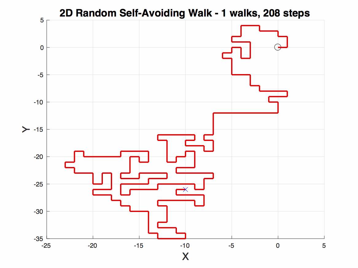
Figure 27: A single trajectory of a 2-dimensional Self-Avoiding Walk (SAW). Whereas a random walk can intersect its path arbitrarily often, a SAW may occupy each site only once. This leads to an increase in the distance between the start and the end, compared to the classic random walk. Self-avoidance has been proposed as the key mechanism driving the drift observed in fixation tasks engbert2011integrated .

Fractional Brownian motion (fBm) is another example. It was introduced by Mandelbrot and van Ness mandelbrot1968fractional to account for processes obeying a scaling law of the functional form $MSD=kt^{2H}$, with $0<H<1,\;\;H\neq\frac{1}{2}$, where $H=\frac{1}{2}$ is the special case of Bm (cfr. Box 12).

It is described by the time-varying pdf

$$P(x,t)=\frac{1}{\sqrt{4\pi Dt^{2H}}}\exp\left[-\frac{x^{2}}{4Dt^{2H}}\right].$$ (97)

fBm has been used as a mathematical reference for random-walk analysis of fixational eye movements (FEMs) and for studying their correlations across time (e.g., engbert2011integrated ). Also, properties of persistence / antipersistence have been exploited, for instance, in analysing optokinetic nystagmus (OKN, trillenberg2001random ).

Case study: random walk analysis of microsaccades

In a number of studies, Engbert and colleagues, e.g., engbert2006microsaccades ; engbert2011integrated ; engbert2012bayesianHurst have shown that a typical trajectory generated by the eyes during FEMs exhibits clear features of a random walk.

For instance, on a short time scale ($2$ to $20$ ms), the RW is persistent, whereas on a long time scale ($100$ to $800$ ms) it exhibits anti-persistent behaviour. Thus, they observed a time-scale separation with two qualitatively different types of motion. On the short time scale, drift produces persistence and this tendency is increased by the presence of microsaccades. On the long time scale, the anti–persistent behaviour is specifically created by microsaccades. Since the persistent behaviour on the short time scale helps to prevent perceptual fading and the anti-persistent behaviour on the long time scale is error-correcting and prevents loss of fixation, they concluded that microsaccade are optimal motor acts to contribute to visual perception

A more recent model of FEMs has also incorporated self-avoidance as the key mechanism driving drifts observed in fixation tasks engbert2011integrated . The Self-Avoiding walk model encodes history by treating space as a lattice and recording the number of visits to each site: the SAW proceeds by choosing the least-visited neighbour at each step. A SAW simulation is provided in Figure 27. The model proposed in engbert2011integrated also includes a confining potential to keep the random walk near the origin, which is needed for the long-time subdiffusive nature of fixation tasks, as well as a mechanism for triggering microsaccades when occupying highly-visited sites.

Case study: optokinetic nystagmus

OKN is a reflexive eye movement with target-following slow phases (SP) alternating with oppositely directed fast phases (FP). For a quick grasp of this kind of eye movement, a video is worth a thousand words, e.g., visit https://www.youtube.com/watch?v=KSJksSA6Q-A. Trillenberg et al trillenberg2001random by measuring FP beginning and ending positions, amplitudes, and intervals and SP amplitudes and velocities, tried to predict future values of each parameter on the basis of past values, using state-space representation of the sequence (time-delay embedding) and local second-order approximation of trajectories. Since predictability is an indication of determinism, this approach allows to investigate the relative contributions of random and deterministic dynamics in OKN. FP beginning and ending positions showed good predictability, but SP velocity was less predictable. FP and SP amplitudes and FP intervals had little or no predictability. FP beginnings and endings were as predictable as randomised versions that retain linear auto-correlation; this is typical of random walks. Predictability of FP intervals did not change under random rearrangement, which also is a characteristic of a random process. They concluded that there is undoubtedly a gross level of deterministic behaviour in OKN. Yet within this range, there is apparently significant random behaviour, with a small amount of predictability. The random behaviour has overlaid on it a form of long-term correlation in the form of anti-persistence. This mixture of dynamics is intriguing and provides a challenge for mathematical modelling efforts, though the physiological meaning of these dynamics is open to conjecture.

Table 16: Power–law distribution

Many empirical quantities cluster around a typical value: speeds of cars on a highway, the temperature in Freiburg at noon in February, etc. Distributions of these quantities place a negligible amount of probability far from the typical value, making the typical value representative of most observations. In short, the underlying processes that generate these distributions fall into the general class well-described by the CLT.

Not all distributions fit this pattern, however, and in some cases the deviation is not a defect or problem, but rather an indication of interesting underlying complexity in the generating process. Complex social, biological and technological systems give rise to countless example of “non-normal” and heavy-tailed distributions. A power-law distribution is one such kind of probability distribution (see Newman newman2005power for a nice review). When the probability of measuring a particular value of some quantity varies inversely as a power of that value, the quantity is said to follow a power law, also known as the Pareto distribution. There are several ways to define them mathematically, one way, for a continuous random variable is the following newman2005power :

$$P(x)=Cx^{-\mu},x\geq x_{min},$$ (98)

where $C=(\mu-1)x_{min}^{\mu-1}$. Note that this expression only makes sense for $\mu>1$, which is indeed a requirement for a power–law form to normalize.

Power–law distributions have many interesting mathematical properties. Many of these come from the extreme right-skewness of the distributions and the fact that only the first $(\mu-1)$ moments of a power-law distribution exist; all the rest are infinite. In general, the $k$-th moment is defined as

$$\langle x^{k}\rangle=\int_{x_{min}}^{\infty}x^{k}P(x)dx=C\int_{x_{min}}^{\infty}x^{-\mu+k}dx=x^{k}_{min}\left(\frac{\mu-1}{\mu-1-k}\right),$$ (99)

with $\mu>k+1$. Thus, when $1<\mu<2$, the first moment (the mean or average) is infinite, along with all the higher moments. When $2<\mu<3$, the first moment is finite, but the second (the variance) and higher moments are infinite! In contrast, all the moments of the vast majority of other pdfs are finite.

Another interesting property of power-law distributions is scale invariance. If we compare the densities at $P(x)$ and at some $P(cx)$, where $c$ is some constant, they are always proportional, i.e. $P(cx)\propto P(x)$. This behaviour shows that the relative likelihood between small and large events is the same, no matter what choice of “small” we make. That is, the density “scales.” It is easy to see that if we take the logarithm of both sides of Eq. (98):

$$\ln P(x)=\ln C-\mu\ln x,$$ (100)

the rescaling $x\rightarrow cx$ simply shifts the power-law up or down on a logarithmic scale. The result shows another well-known property of a power-law distribution: it appears as a straight line on a $\log-\log$ plot, as opposed to the strongly curved behaviour of an exponential distribution (see Fig. 28).

Inspiring analyses of eye movements and visual search in terms of power–law behaviour and power spectra have been conducted by Deborah Aks et al. aks2002memory suggesting that our oculomotor system may produce a complex and self-organising search pattern providing maximum coverage with minimal effort.

t] .

Figure 28: Exponential distribution $P(x)\propto e^{-\alpha x}$ (top-left) vs. power–law distribution $P(x)\propto x^{-\mu}$ (top-right): pdf shapes look apparently similar. However, the exponential pdf is represented as a straight line on a semilog graph of $\log P(x)$ versus $x$ (bottom-left), whilst the power-law shapes as a straight line on a log-log graph (bottom-right), a signature of the heavy-tail behaviour

7.2 A second violation: loosing your moments

Even in the absence of correlations, a mechanism for disrupting convergence to Brownian motion in the long time limit is using power–law tailed distributions in the random walk steps (i.e., power–law distributed noise rather than Wiener or similar noise). Lévy flights (LFs) are one such mechanism. LFs are stochastic processes characterised by the occurrence of extremely long jumps, so that their trajectories are not continuous anymore. The length of these jumps is distributed according to a Lévy stable statistics with a power–law tail and divergence of the second moment. This peculiar property strongly contradicts the ordinary Bm, for which all the moments of the particle coordinate are finite.

t]

Figure 29: Different 2-dimensional $\alpha$-stable motions obtained by sampling the “noise” component $\bm{\xi}\sim f(\bm{\xi};\alpha,\beta,\gamma,\delta)$ in Eq. (102) for different values of the characteristic index parameter $\alpha$. The plots shown in the four panels – left to right, top to bottom –, have been generated via $\alpha=1,\alpha=1.2,\alpha=1.5,\alpha=2$, respectively. The same number of discrete steps ($\#500$) has been fixed for all the examples, but note how the “scale” of the exploration restricts as $\alpha\rightarrow 2$, eventually reaching the limit case $\alpha=2$ where classic Bm is generated (bottom right plot).

For a random walker who takes steps of size $l$ according to a probability density function

$$P(l)\approx l^{-\mu},$$ (101)

the resulting type of diffusion depends on the value of $\mu$. In particular:

a) $\mu>3$:

the CLT guarantees convergence to normal diffusion and Brownian regime holds;

b) $\mu\to 1$:

the ballistic motion limit is reached;

c) $1<\mu<3$:

superdiffusive behaviour occurs.

LFs arise in the super diffusive regime, when the jump size distribution has a power–law tail with $\mu<3$. As discussed in Box 16, for such values of the power–law exponent, the RVs can have diverging variance. The necessary and sufficient conditions of the classical CLT do not hold in this case. Lévy flight patterns comprise sequences of randomly orientated straight-line movements. Frequently occurring but relatively short straight-line movement randomly alternate with more occasionally occurring longer movements, which in turn are punctuated by even rarer, even longer movements, and so on with this pattern repeated at all scales. Some examples of LF patterns are provided in Figure 29. As a consequence, the straight-line movements have no characteristic scale, and LFs are said to be scale-free.

At the microscopic level, the simulation of individual LF trajectories do not require complex calculations to execute. They are a Markovian process and can be easily obtained from Eq. (54), by setting $\mathbf{A}=0$

$$d\mathbf{x}(t)={\mathbf{B}}({\mathbf{x}},t)\bm{\xi}(t)dt={\mathbf{B}}({\mathbf{x}},t)d{\mathbf{L}_{\alpha}}(t)$$ (102)

The form of this equation is that of the Wiener process, however in this case the stochastic increment $d{\mathbf{L}_{\alpha}}(t)=\bm{\xi}(t)dt$ is sampled from an $\alpha$-stable distribution $f(\bm{\xi};\alpha,\beta,\gamma,\delta)$ (cfr. Box 17):

$$\bm{\xi}(t)\sim f(\bm{\xi};\alpha,\beta,\gamma,\delta).$$ (103)

In other terms, $d{\mathbf{L}_{\alpha}}(t)$ in the context of Eq. (102) represents an infinitesimal Lévy motion.

The macroscopic description of the pdfs for particles undergoing a Lévy flight can be modeled using a generalised version of the Fokker-Planck equation. The equation requires the use of fractional derivatives and we will not discuss it here since really beyond the scope of an introductory chapter.

By discretising and iterating Eq. (102), over a large number of trials a Lévy flight will be distributed much farther from its starting position than a Brownian random walk of the same length (see again Figure 29). Indeed, the $MSD$ of a Brownian walker has a linear dependence on time whereas that of a Lévy flier grows faster and depends on time raised to some power $>1$. This result gives a precise meaning to their characterisation as “super-diffusive.” The probability density function for the position of the walker converges to a Lévy $\alpha$-stable distribution with Lévy index $\alpha=\mu-1$, with $0<\alpha\leq 2$ (with the special case $\alpha=2$ corresponding to normal diffusion). The Lévy index is an important feature. For instance, it has been shown that it is suitable to characterise the variation or activity of fMRI signals of different networks in the brain under resting state condition. Visual and salience networks seem to present a definite Lévy motion-like behaviour of activity, whereas areas from the cerebellum exhibit Brownian motion costa2016foraging .

The Hurst exponent $H$, the characteristic index $\alpha$, and the power–law exponent $\mu$ are related as follows:

$$H=\frac{1}{\alpha}=\frac{1}{\mu-1}.$$ (104)

Thus, rephrasing the conditions that have been discussed for the $\mu$ exponent, for $\alpha<2$ one cannot define the MSD because it diverges. Instead, one can study moments of order lower than $\alpha$ because they do not diverge. Nevertheless, one can define some “empirical” width, such as half widths at half maximum, and show that a pseudo-MSD grows as $\approx t^{\frac{1}{\alpha}}$ for Lévy flights.

Table 17: Stable distributions

The family of $\alpha$-stable distributions gnedenko1954limit form a four-parameter family of continuous probability densities, say $f(\bm{\xi};\alpha,\beta,\gamma,\delta)$. The parameters are the skewness $\beta$ (measure of asymmetry), the scale $\gamma$ (width of the distribution) and the location $\delta$ and, most important, the characteristic exponent $\alpha$, or index of the distribution that specifies the asymptotic behaviour of the distribution. The relevance of $\alpha$ derives from the fact that the pdf of jump length scales, asymptotically, as $l^{-1-\alpha}$. Thus, relatively long jumps are more likely when $\alpha$ is small. By sampling $\bm{x}\sim f(\bm{x};\alpha,\beta,\gamma,\delta)$, for $\alpha\geq 2$ the usual Bm occurs; if $\alpha<2$ , the distribution of lengths is “broad” and the so called Lev́y flights take place.

One example of $\alpha$-stable motions generated for varying the $\alpha$ index is illustrated in Fig. 29.

A random variable $X$ is said to have a stable distribution if: (1) the parameters of its probability density function $f(x;\alpha,\beta,\gamma,\delta)$ are in the following ranges $\alpha\in\left(0;2\right]$, $\beta\in\left[-1;1\right]$, $\gamma>0$, $\delta\in\mathbb{R}$ and (2) if its characteristic function $E\left[\exp(itx)\right]=\int_{\mathbb{R}}\exp(itx)dF(x)$, $F$ being the CDF, can be written as

$$E\left[\exp(itx)\right]=\begin{cases}\exp\left[-|\gamma t|^{\alpha}\left(1-i\beta\frac{t}{|t|})\tan(\frac{\pi\alpha}{2}\right)+i\delta t\right]\\ \exp\left[-|\gamma t|\left(1+i\beta\frac{2}{\pi}\frac{t}{|t|}\ln|t|\right)+i\delta t\right]\end{cases}$$

The first expression holds if $\alpha\neq 1$, the second if $\alpha=1$.

Special cases of stable distributions whose pdf can be written analytically, are given for $\alpha=2$, the Normal distribution with

$$f(x;2,0,\frac{\sigma}{\sqrt{2}},\mu)=\mathcal{N}(x;\mu,\sigma^{2}),$$ (105)

for $\alpha=1$, the Cauchy or Lorentz distribution

$$f(x;1,0,\gamma,\delta)=\frac{1}{\pi\gamma}\left[\frac{\gamma^{2}}{(x-\delta)^{2}+\gamma^{2}}\right],$$ (106)

and for $\alpha=0.5$, the Lévy distribution

$$f(x;0.5,1,\gamma,\delta)=\sqrt{\frac{\gamma}{2\pi}}\frac{\exp{-(\frac{\gamma}{2(x-\delta)})}}{(x-\delta)^{3/2}}.$$ (107)

For all other cases, only the characteristic function is available in closed form, and numerical approximation techniques must be adopted for both sampling and parameter estimation chamb ; nolan1997 ; koutrouvelis1980 . A very nice and simple to use Matlab package for parameter inference and computation of $\alpha$-stable distributions is freely downloadable at Mark Veilette’s homepage http://math.bu.edu/people/mveillet/html/alphastablepub.html.

Some examples of $\alpha$-stable pdfs and related complementary cumulative distribution function (CCDF) are given in Fig.30. The use of the CCDF, or upper tail, of jump lengths is the standard convention in the literature, for the sake of a more precise description of the tail behaviour, i.e. the laws governing the probability of large shifts. The CCDF is defined as $\overline{F}_{X}(x)=P(X>x)=1-F_{X}(x)$, where $F_{X}(\cdot)$ is the CDF (cfr., Box 13).

t]

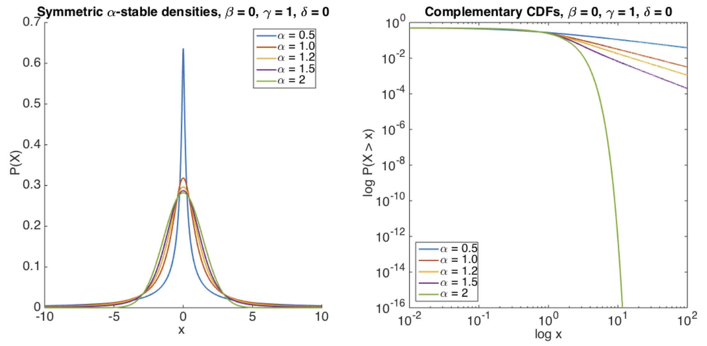
Figure 30: Plots of symmetric $\alpha$-stable distributions (left) and their complementary CDF (CCDF) on $\log-\log$ axes (right) for different values of the characteristic index parameter $\alpha=0.5,1,1.2,1.5,2$. The CCDF shows the rapid fall-off of the tail of the Gaussian case ($\alpha=2$) as opposed to the power–law tail behaviour of actual Lévy flights $\alpha<2$

Case study: the Lévy flight of saccades

Brockmann and Geisel brockgeis have assumed a power–law dependence in the tail of the saccade amplitude distribution, for which they found empirical support in free viewing of natural scenes. Minimisation of the time needed to scan the entire visual space then led them to predict that eye movement trajectories behave as Lévy flights, as opposed to more common diffusive random walks, which would result from a Gaussian amplitude distribution. But in order to obtain simulated eye trajectories that look like their observed scan paths, an empirical determination of a salience field for the correspondingly viewed scene is still needed. Brockmann and Geisel derived that salience field from the spatial distribution of fixations made by observers throughout the scene (a picture of a party). As to the amplitude distribution they considered the Cauchy distribution (Eq. 106)

The stochastic assumptions of saccade generation made by Brockmann and Geisel brockgeis involve a Markovian process, consistent with an interpretation of visual search originally proposed by Horowitz and Wolfe horowitz1998visual . However, the predictions and results of the Brockmann and Geisel model do not change substantially if those assumptions are relaxed so as to allow a sufficiently rapidly decaying correlation in the saccade sequences.

Further evidence and characterisation of L vy-like diffusion in eye movements associated with spoken-language comprehension have recently been provided by Stephen, Mirman, Magnuson, and Dixon stephen2009 .

Case study: the microsaccade conundrum

Martinez-Conde and colleagues martinez2013impact ; otero2013oculomotor have put forward the proposal that microsaccades and saccades are the same type of eye movement (the “continuum hypothesis”). The microsaccade–saccade continuum is sustained by evidence that saccades of all sizes share a common generator

In this respect, a straightforward hypothesis on the function microsaccades is that they help to scan fine details of an object during fixation. This hypothesis would imply that fixational eye movements represent a search process. According to this analogy, the statistics of microsaccades can be compared to other types of random searches, namely inspection saccades during free picture viewing brockgeis .

Given these assumptions, Engbert et al. engbert2006microsaccades checked whether the amplitude distribution of microsaccades and saccades follows a similar law.

To investigate the distribution of microsaccade amplitude in a data set of $20,000$ microsaccades, they analysed the tail of the distribution on a double logarithmic scale. They obtained a power–law decay of the tail with exponent $\mu=4.41$, which would reject the hypothesis of a Lévy flight for microsaccades (requiring $\mu<3$), if compared with numerical results obtained by Brockmann and Geisel brockgeis . In turn, this apparently would also lead to reject the “continuum hypothesis”. However there are many subtleties that should be taken into account in order to fairly compare two such different analyses (e.g., sampling rate and discretisation of the eye tracking raw data) before reaching a conclusion. But at least this nice piece of work is useful to show how advanced statistical methods for eye movement analysis can address big questions in the field.

t]

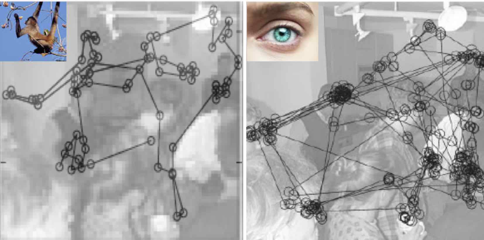
Figure 31: Monkey or human: can you tell the difference? The left image has been obtained by superimposing a typical trajectory of spider monkeys foraging in the forest of the Mexican Yucatan, as derived from ramos2004levy , on the “party picture” used in brockgeis . The right image is an actual human scan path (modified after brockgeis )

7.3 The foraging perspective

Consider Fig. 31: prima facie, is seems to illustrate a bizarre jest. However, from eye-movements studies canosa2009real ; tatler2006long ; tatler2008systematic ; tatler2009prominence ; dorr2010variability ; over2007coarse ; TatlerBallard2011eye , there is evidence that eye movement trajectories and their statistics are strikingly similar, with respect to the resulting movement patterns and their statistics to those exhibited by foraging animals, viswa08 ; codling2008 ; plank2008 ; reynolds2008optimal . In other terms, eye movements and animal foraging address in some way a similar problem brockgeis . Under the foraging metaphor, the eye (and the brain modules controlling the eye behaviour) is the forager, the input visual representation $\mathcal{D}$ is the foraging landscape. Points attracting fixations are foraging sites (in the case of static images) or moving preys (time-varying scenes); gaze shifts occur due to local exploration moves, prey pursuit and long relocation from one site to another.

An intriguing issue is whether the foraging theory underpinning the proposed analyses just provides a useful computational theory metaphor, or constitutes a more substantial ground. Interestingly enough, Hills hills2006animal has argued that what was once foraging in a physical space for tangible resources became, over evolutionary time, foraging in cognitive space for information related to those resources. Adaptations that were selected for during ancestral times are, still adaptive now for foraging on the internet or in a supermarket, or for goal-directed deployment of visual attention wolfe2013time . In these terms, the foraging approach may set a broader perspective for discussing fundamental themes in eye movement behaviour, e.g., the “continuum hypothesis” of Martinez-Conde and colleagues martinez2013impact ; otero2013oculomotor .

Building on this rationale, gaze shift models have been proposed coping with different levels of visual representation complexity bfpha04 ; BocFerAnnals2012 ; BocFerSPIC2012 ; BocFerSMCB2013 ; BocCOGN2014 ; napboc_TIP2015 and eye movement data analyses have been performed in terms of foraging efficiency wolfe2013time ; cain2012bayesian .

More formally, rewrite the 2-dimensional Langevin equation (54), interpreting the deterministic component $\mathbf{A}(\mathbf{x},t)$ as an external force field due to a potential $V(\mathbf{x},t)$ bfpha04 (see Fig. 32), that is $\mathbf{A}(\mathbf{x},t)=-\nabla V(\mathbf{x},t)$, where the “del” (or “nabla”) symbol $\nabla$ denotes the gradient operator.

Then,

$$d\mathbf{x}(t)=-\nabla V(\mathbf{x},t)dt+{\mathbf{B}}({\mathbf{x}},t)d{\mathbf{L}_{\alpha}}(t).$$ (108)

Equation (108) now provides a microscopic description (trajectory) of a RW biased by an external force field.

We can thus generalise to two dimensions the discretisation method used to obtain the $1-$dimensional Eq (66) so to gain an operative definition of the SDE (108)

$$\overbrace{\mathbf{x}_{i+1}}^{\text{new gaze location}}=\overbrace{\mathbf{x}_{i}}^{\text{current gaze location}}-\overbrace{\nabla V(\mathbf{x_{i}},t_{i})\Delta t_{i}}^{\text{external force}}+\overbrace{{\mathbf{B}}({\mathbf{x}}_{i},t_{i})(\Delta t_{i})^{\frac{1}{\alpha}}\bm{\xi}_{i}}^{\text{L\'{e}vy motion}}$$ (109)

which makes clear that next gaze position is obtained by shifting from current gaze position following a Lévy displacement that is constrained by the external potential field. The external potential summaries the informative properties of the “visual landscape” of the forager.

For instance in bfpha04 Eq. (109) was used as a generative model of eye movements. In that case, the external potential was taken as a function of the salience field and $\bm{\xi}_{i}$ was sampled from a Cauchy distribution. Each sampled gaze shift was then accepted according to a Metropolis-like algorithm (cfr. Box 4), governed by a “temperature” parameter suitable to tune the randomness of the visual exploration (i.e., the attitude of the forager to to frequently engage in longer relocations/saccade rather then keeping with local/fixational exploration). One example is provided in Fig. 32.

As to the parameters of Eq. (109), it is worth noting that established numerical techniques are available for fitting such parameters from real data (see, e.g. siegert2001 ). Once the parameters have been learned, the generative capabilities of Eq. (109) can be straightforwardly used to Monte Carlo simulate gaze shifts whose characteristics can then be compare with human data. For instance in a recent paper by Liberati et al. LiberatiASD2017 , it is shown that scan paths of children with typical development (TD) and Autism Spectrum Disorder (ASD) can be characterised by eye movements geometrically equivalent to Lévy flights, but with a different degree of randomness, which can be captured by a temperature parameter as in bfpha04 .

As previously discussed, the heavy-tailed distributions of gaze shift amplitudes are close to those characterising the foraging behaviour of many animal species. Lévy flights have been used to model optimal searches of foraging animals, namely their moment-to-moment relocations/flights used to sample the perceived habitat viswa08 . However, the general applicability of Lévy flights in ecology and biological sciences is still open to debate. In complex environments, optimal searches are likely to result from a composite strategy, in which Brownian and Lev́y motions can be adopted depending on the structure of the landscape in which the organism moves plank2008 . Lévy flights are best suited for the location of randomly, sparsely distributed patches and Brownian motion gives the best results for the location of densely but random distributed within-patch resources reynolds2008many .

t]

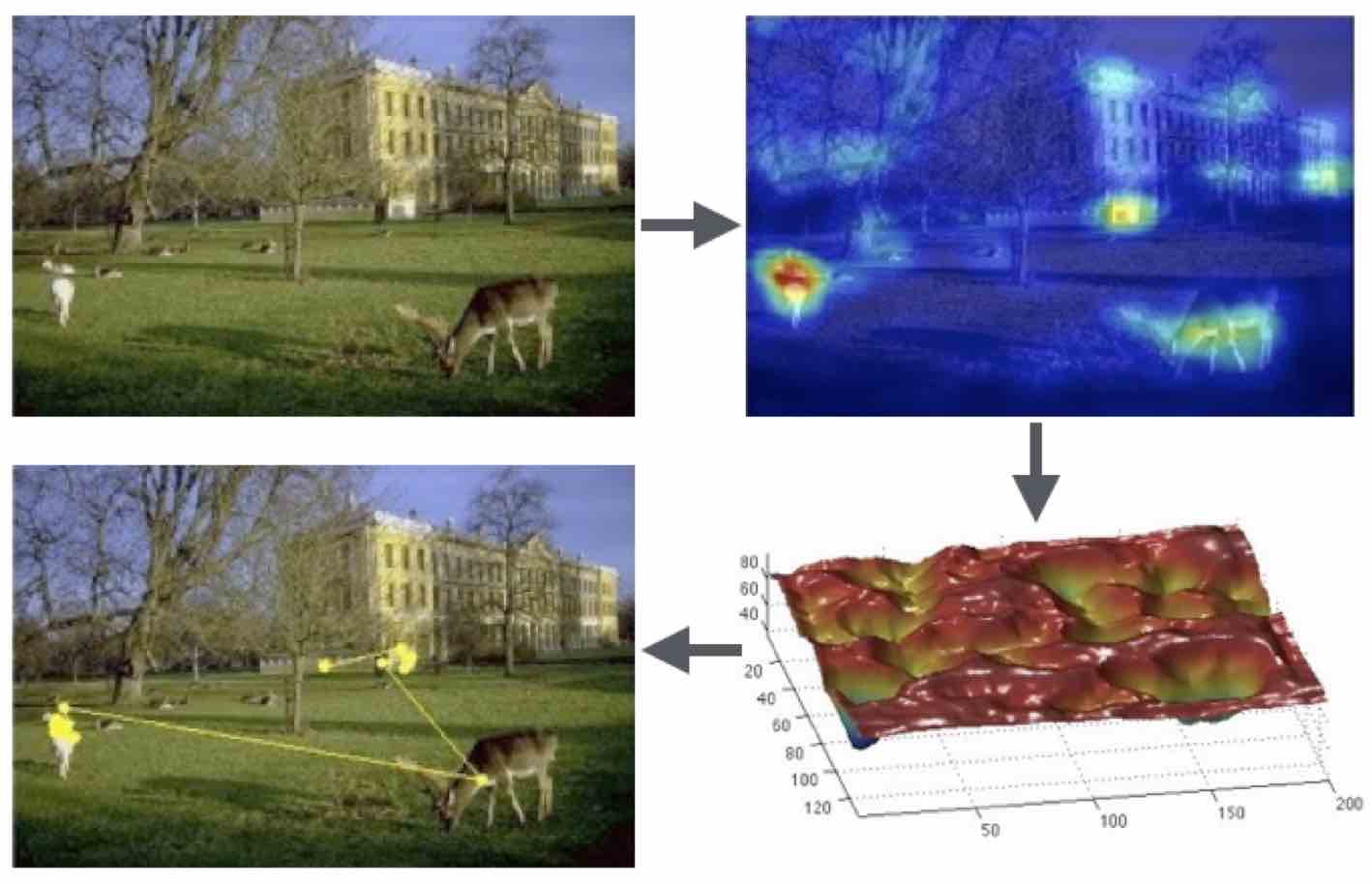
Figure 32: The Lévy model used as a generative model. Top left: the original image. Top right: the salience map. Bottom right: the potential $V(\mathbf{x_{i}},t_{i})$ computed from saliency: potential wells represent informative regions that can attract gaze. Bottom, left: the final scan path superimposed on the original image.

Also it is possible to compose the strategy as a hybrid strategy in which Brownian-like motion is adopted for local exploration (e.g., FEMs and small saccades) and Lévy displacements are exploited for long relocations (medium / long saccades) A preliminary attempt towards such a composite strategy for modelling gaze shift mechanisms has been presented in BocFerIciap2011 . However, that approach only conjectured a simple binary switch between a Gaussian and a Cauchy-like walk. In BocFerSMCB2013 the approach was generalised to handle observers watching videos and thus accounting for multiple kinds of shifts: FEMs, saccade and smooth pursuit (cfr. Fig. 33). To this end, Eq. (109) is reformulated as a 2-dimensional dynamical system in which the stochastic part is driven by one-of-$K$ possible types of $\alpha$-stable motion $\bm{\xi}_{i}^{k}$.

t]

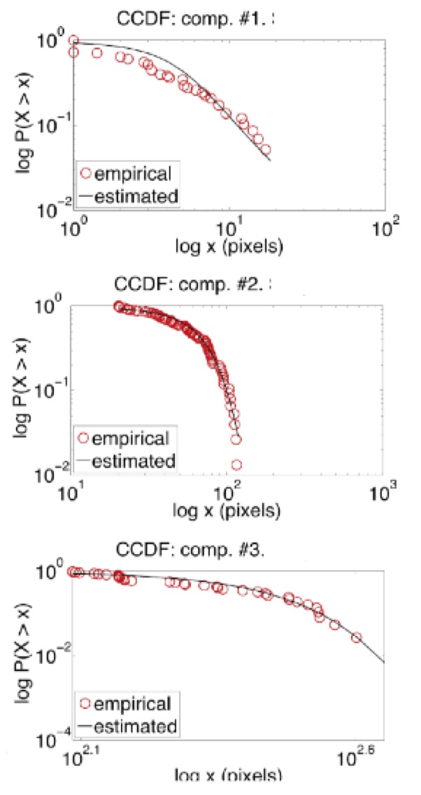
Figure 33: Analysis of gaze shift dynamics from a video. The different components were automatically separated by using a clustering procedure based on the Variational Expectation-Maximization algorithm (see BocFerSMCB2013 for details). Then, each component was fitted by an $\alpha$-stable distribution. Fitting results for one eye-tracked subject are shown in terms of double log plot of the CCDF. From top to bottom: first component accounting for smooth-pursuit and FEMs motions; the medium saccade component; the long saccade component

In the Ecological Sampling model BocFerSMCB2013 the switch from one motion type to the other was bottom-up determined as a multinomial choice biased by the complexity of the sampled visual landscape. More recently this idea was extended to a top-down and task-dependent probabilistic choice in the framework of Bayesian Decision theory BocCOGN2014 . Bayesian Decision theory has gained currency in modelling active sensing behaviour yang2016theoretical : though minimal, from a theoretical standpoint, a gaze shift action can indeed be considered as the result of a decision-making process (either conscious or uncounscious).

8 From patterns of movement to patterns of the mind: unveiling observer’s hidden states

The last point we are addressing in this Chapter is: can we infer target hidden states of observer’s mind by analysing his eye movement trajectories? Or, in foraging terms, can we say something on forager’s internal state by observing his foraging patterns?

Generally speaking, the hidden states that we may target could be, for example, the task the observer is accomplishing, his expertise, his emotional state (but, also, a certain pathology affecting a group of patients as opposed to a control group).

More formally, if $\mathbf{T}$ denotes the target internal state (or a set of states) and $\mathbf{X}$ the visible eye movement behaviour, e.g., $\mathbf{X}=\{\mathbf{x}_{F}(1),\mathbf{x}_{F}(2),\cdots\}$, (or, alternatively, the sequence of gaze, amplitudes, directions and durations), one can assume a generative process $\mathbf{T}\rightarrow\mathbf{X}$, where the observer’s hidden state shapes the kind of eye trajectories.

In probabilistic terms the generative process can be captured by the simple PGM sketched in Fig. 34, which factorises the joint pdf $P(\mathbf{T},\mathbf{X})$ as $P(\mathbf{T},\mathbf{X})=P(\mathbf{X}\mid\mathbf{T})P(\mathbf{T})$ (product rule).

t]

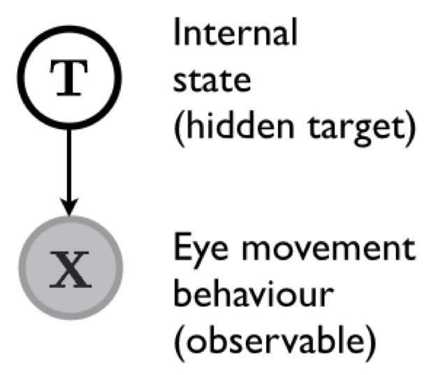
Figure 34: The PGM specifying the generative process $\mathbf{T}\rightarrow\mathbf{X}$ through the joint pdf factorisation: $P(\mathbf{T},\mathbf{X})=P(\mathbf{X}\mid\mathbf{T})P(\mathbf{T})$. The shaded node denotes that RV $\mathbf{X}$ is observable

This way, anything we can infer on the hidden state given the observable behaviour is obtained by “inverting the arrow”, i.e., by applying Bayes’ rule:

$$P(\mathbf{T}\mid\mathbf{X})=\frac{P(\mathbf{X}\mid\mathbf{T})P(\mathbf{T})}{P(\mathbf{X})}.$$ (110)

Once the posterior has been computed, then we use decision theory to determine output $\mathbf{T}=t$ for each new input $\mathbf{X}=\mathbf{x}$

Note that this is a very general formulation of the problem, which actually may entail a large number of solutions, and the PGM shown in Figure 34 could be further specified/specialised in number of ways. Also, to keep the description simple, we have omitted the set of parameters involved by the actual specification of the pdfs in Eq. (110). Clearly, before Eq. (110) can be put into work, such parameters are to be specified and fitted, or, adopting a more modern term, learned. To this end, a huge amount of Machine Learning (ML) techniques are today available (see Box 18, for ML basic terminology in a nutshell, and BishopPRML ; murphy2012machine for an in-depth presentation)

Keeping to such general level, from a methodological standpoint there are at least three distinct approaches to cope with the inverse inference problem posed by Eq.( 110). In decreasing order of complexity:

1. First solve the inference problem of determining the likelihood function $P(\mathbf{X}\mid\mathbf{T})$ and the prior probabilities $P(\mathbf{X})$. Then use Bayes’ theorem in the form given in Eq. (110). Equivalently, we can model the joint distribution $P(\mathbf{T},\mathbf{X})$ directly and then normalise to obtain the posterior probabilities $P(\mathbf{T},\mathbf{X})$. Approaches that explicitly or implicitly model the distribution of inputs as well as outputs are known as generative models, because by sampling from them it is possible to generate synthetic data points in the input space. The popular Naive Bayes and Linear Discriminant Analysis methods are very simple instances (though effective in many practical cases) of a generative approach; Hidden Markov Models (HMM) BishopPRML ; murphy2012machine for modelling time series provide an appealing example of a generative approach that has been often exploited for eye movement analysis.

2. Solve straightforwardly the inference problem of determining the posterior probabilities $P(\mathbf{T},\mathbf{X})$, and then subsequently use decision theory to assign each new $\mathbf{X}=\mathbf{x}$ to an output target. Approaches that model the posterior probabilities directly are called discriminative models. Logistic regression is one notable and classic example, Conditional Random Fields (CRFs) for modelling time series are more sophisticated one BishopPRML ; murphy2012machine .

3. Find a function $f:\mathbf{X}\to\mathbf{T}$, called a discriminant function, which maps each input $\mathbf{X}=\mathbf{x}$ directly onto a class label. For instance, in the case of two-class problems, e.g., distinguishing experts from novice observers, $\mathbf{T}$ might be binary valued and such that $f=0$ represents class $\mathbf{T}=t_{1}$ and $f=1$ represents class $\mathbf{T}=t_{2}$. In this case, probabilities play no role. Many popular artificial neural nets or modern methods such as the Support Vector Machine (SVM) for regression and classification (a baseline technique in ML) implement this approach BishopPRML ; murphy2012machine .

Note that, since many applications require a posterior class probability, methods based on discriminant functions can be “transformed” into discriminative ones in order to gain an output in probabilistic form. For instance, the output $f(\cdot)$ of a binary SVM classifier can be fed into a sigmoid function, to approximate the posterior (e.g., $P(\mathbf{t}\mid\mathbf{X})\approx\frac{1}{1+\exp(Af+B)}$, where $A,B$ are parameters that can be determined via regularised maximum likelihood).

Clearly, the generative approach is in principle the most appealing one. However it should be recalled that apart from simple cases such as Naïve Bayes (see Box 19), the normalisation of the joint pdf can be a hard task. Referring again to Eq. (110), calculating the normalisation factor $P(\mathbf{X})$ requires the marginalisation $P(\mathbf{X})=\sum_{\mathbf{T}}P(\mathbf{T},\mathbf{X})$ ($P(\mathbf{X})=\int P(\mathbf{T},\mathbf{X})d\mathbf{T}$ when RVs are continuous), which, in real cases, is hardly computable. Thus, complex approximation techniques such as Monte Carlo or Variational Bayes are to be taken into account BishopPRML ; murphy2012machine .

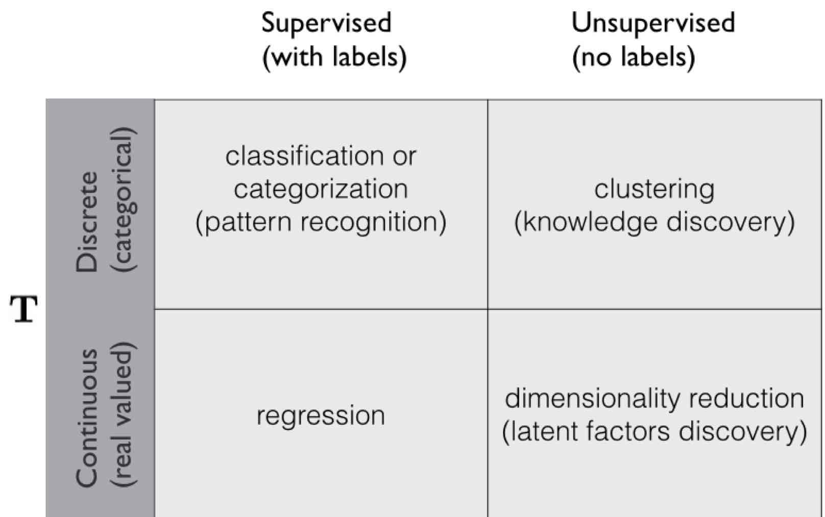
Figure 35: The main problems Machine Learning is addressing

Table 18: Machine Learning in a nutshell

In the inferential process defined by Eq. ( 110), $\mathbf{T}$ represents the output of the process and $\mathbf{X}$ the given input. In Statistical Machine Learning (briefly, ML) terminology $\mathbf{X}$ is usually shaped as a random vector of features (or attributes, or covariates), $\mathbf{X}=\{\mathbf{X}_{i}\}_{i=1}^{N}$, where $i$ is a suitable index. For example when $i$ is a time index, then $\{\mathbf{x}_{1},\mathbf{x}_{2}\}$ is the realisation of a stochastic process. ML does not relate to a specific problem thus $\mathbf{X}_{i}$ could be a complex structured object, such as an image, a sentence, an email message, a graph, etc.

The form of the output or response variable $\mathbf{T}$ can be either discrete (categorical, nominal) or continuous (real-valued). One example of the first type, is when $\mathbf{T}$ can take the label of one of two tasks given to the observer, e.g., $\mathbf{T}=t_{k}$ where $t_{1}=\text{``look for people''}$ and $t_{2}=\text{``look for cars''}$. Another example, is $\mathbf{T}$ taking values over the discrete set of basic emotion (“fear”, “disgust”, “joy”, etc.). As opposed to this latter example, we could try instead, to infer from eye movements a continuous affect state, so that $\mathbf{T}$ is taking values $t_{i}$ in the real valued space of valence and arousal.

From a practical standpoint, when using a ML approach to analyse our eye tracking data we can be in one of these two conditions:

1. supervised learning: we know where input $\mathbf{x}_{i}$ comes from (e.g., $\mathbf{x}_{i}$ was measured while the observer was scanning a happy face); more formally $\mathbf{x}_{i}$ is paired with target value or label $t_{i}$, thus we have a training set $\mathcal{D}=\{(\mathbf{x}_{i},t_{i})\}_{i=1}^{N}$;

2. unsupervised learning: we have no labels, and our dataset is represented by the bare input data $\mathcal{D}=\{(\mathbf{x}_{i})\}_{i=1}^{N}$

Thus, in the supervised setting the goal is to learn a mapping from input $\mathbf{X}$ to output $\mathbf{T}$, given a labeled set of input-output pairs. When $\mathbf{T}$ is discrete the problem is known as classification or pattern recognition; when $\mathbf{T}$ is real-valued, we are performing regression.

In the unsupervised setting, we have no labels available, thus the goal is to find “interesting patterns” in the data. This is sometimes named knowledge discovery or data mining. It is a much less well-defined problem, since we are not told what kinds of patterns to look for, and there is no obvious error metric to use (unlike supervised learning, where we can compare our prediction for a given x to the observed value). When $\mathbf{T}$ is discrete, the problem is known as clustering. When $\mathbf{T}$ is real-valued we are typically in the case of dimensionality reduction. The latter is used when dealing with high dimensional data: it is often useful to reduce the dimensionality by projecting the data to a lower dimensional subspace which captures the “essence” of the data. Indeed, although the input data may appear high dimensional, there may only be a small number of degrees of variability, corresponding to latent factors (Principal Component Analysis or Factor Analysis being well known examples).

Statistical Machine Learning is nowadays a broad and mathematically sophisticated field. Two excellent and up-to-date textbooks are those by Bishop BishopPRML and Murphy murphy2012machine .

8.1 Inverting Yarbus to infer the task

We now assume that the target internal state $\mathbf{T}$ of the observer stems from a given visual task, and for simplicity we straightforwardly use $\mathbf{T}$ to denote the task. In other terms, the task $\mathbf{T}$ is the hidden state of interest.

The seminal experiment by Yarbus Yarbus studied the effect of the visual task on the trajectories of eye movements $\mathbf{X}$. On the basis of our introductory discussion, we know that in probabilistic terms the effect $\mathbf{T}\rightarrow\mathbf{X}$, or forward mapping, is formally captured by the likelihood function $P(\mathbf{X}\mid\mathbf{T})$. Also, we know that Eq. (110) is an application of Bayes’ rule, to compute the posterior probability of the task $\mathbf{T}$ after having observed eye movement trajectories $\mathbf{X}$. Summing up, the inference of the task requires the computation of the inverse mapping $\mathbf{T}\leftarrow\mathbf{X}$, which is easily understood as an “inverse Yarbus” process haji2013computational .

Clearly, as previously mentioned, there are several ways of “inverting Yarbus”.

Case study: Inverting Yarbus via Naïve Bayes

In a recent study henderson2013predicting , Henderson et al. considered four tasks: scene search, scene memorisation, reading, and pseudo-reading. Task inference was achieved by classifying the observers’ task by implementing Eq. (110) as the baseline Naïve Bayes’ (NB) classifier. Namely they addressed two problems: (i) whether the task associated with a trial could be identified using training from other trials within the same experimental session (within-session classification); (ii) whether the task performed in one session could be identified based on training from a session conducted on a different day (cross-session classification). Twelve members of the University of South Carolina community participated in the experiment. A dedicated classifier was trained for each observer, thus the baseline NB has proved to be sufficient. NB classifiers were trained on a feature vector $\mathbf{X}$ of dimension $8$, i.e., eight eye movement features capturing eye movement patterns for each trial: the mean and standard deviation of fixation duration, the mean and standard deviation of saccade amplitude, the number of fixations per trial, and the three parameters $\mu$, $\sigma$, and $\tau$ quantifying the shape of the fixation duration distribution with an ex-Gaussian distribution, which is known to change for different eye-movement tasks (cfr., henderson2013predicting for details.

Table 19: Naïve Bayes

The Naïve Bayes algorithm is a classification algorithm based on Bayes rule, that assumes the attributes $\mathbf{X}=\{\mathbf{X}_{1},\mathbf{X}_{2},\cdots\}$ are all conditionally independent of one another given $\mathbf{T}$. Consider, for example, the two feature case, where $\mathbf{X}=\{\mathbf{X}_{1},\mathbf{X}_{2}\}$, then

$$P(\mathbf{X}\mid\mathbf{T})=P(\mathbf{X}_{1},\mathbf{X}_{2}\mid\mathbf{T})=P(\mathbf{X}_{1}\mid\mathbf{X}_{2},\mathbf{T})P(\mathbf{X}_{2}\mid\mathbf{T})=P(\mathbf{X}_{1}\mid\mathbf{T})P(\mathbf{X}_{2}\mid\mathbf{T})$$ (111)

Thus, if $\mathbf{X}$ contains $n$ attributes: $P(\mathbf{X}\mid\mathbf{T})=\prod_{i=1}^{n}P(\mathbf{X}_{i}\mid\mathbf{T})$. This way Eq. 110 can be written as

$$P(\mathbf{T}=t_{k}\mid\mathbf{X})=\frac{P(\mathbf{T}=t_{k})\prod_{i=1}^{n}P(\mathbf{X}_{i}\mid\mathbf{T}=t_{k})}{\sum_{j}P(\mathbf{T}=t_{j})\prod_{i=1}^{n}P(\mathbf{X}_{i}\mid\mathbf{T}=t_{j})}.$$ (112)

If we are interested only in the most probable value of $\mathbf{T}$, then we have the Naïve Bayes classification/decision rule: $\mathbf{T}\leftarrow\arg\max_{t_{k}}P(\mathbf{T}=t_{k}\mid\mathbf{X})$, which simplifies Eq. (112) to the following (because the denominator does not depend on $t_{k}$ ):

$$\mathbf{T}\leftarrow\arg\max_{t_{k}}P(\mathbf{T}=t_{k})\prod_{i=1}^{n}P(\mathbf{X}_{i}\mid\mathbf{T}=t_{k})$$ (113)

Case study: Inverting Yarbus via HMM

In haji2013computational Haji-Abolhassani and Clark present a study in which Eq. (110) is shaped to explicitly account for the gaze shift sequence as a stochastic process. They present different experiments and models, but here, for clarity sake, we will consider a basic condition and a baseline model so to capture the rationale behind their approach and, also, to compare with the Ellis and Stark model presented in Section 6.2. Recall that in that case the transition matrix $A_{kj}$ was directly estimated by “counting” the percentage of transitions from one point of interest to another (more formally, via Maximum Likelihood estimation). Thus, the model was an observable Markov model. In the inverse Yarbus setting, it can be represented as the Markov chain conditioned on task $\mathbf{T}$ that is depicted in Fig.  37 (top panel, solution $1$). Different tasks are likely to give rise to different transition matrices. In haji2013computational visual tasks considered in the simplest experiment were counting red bars, green bars, blue bars, horizontal bars, vertical bars, or characters.

Even if we leave apart subtle issues such as the dissociation between the centre of gaze and the covert focus of attention haji2013computational , it is very unlikely for a saccade to land exactly on the chosen point of interest (objects or salient locations). The fixation locations may undershoot or overshoot the targets due to oculomotor properties of human eyes or the noisiness of the eye tracker. To account for this problem, in terms of an observable Markov model, a “practical” viable solution is to relax the exact point of interest condition to a more flexible region of interest surrounding the point. This indeed was the solution adopted by Stark and colleagues hacisalihzade1992visual ; ellistark , depicted in Fig. 17, and which we now recall in Fig. 36.

t]

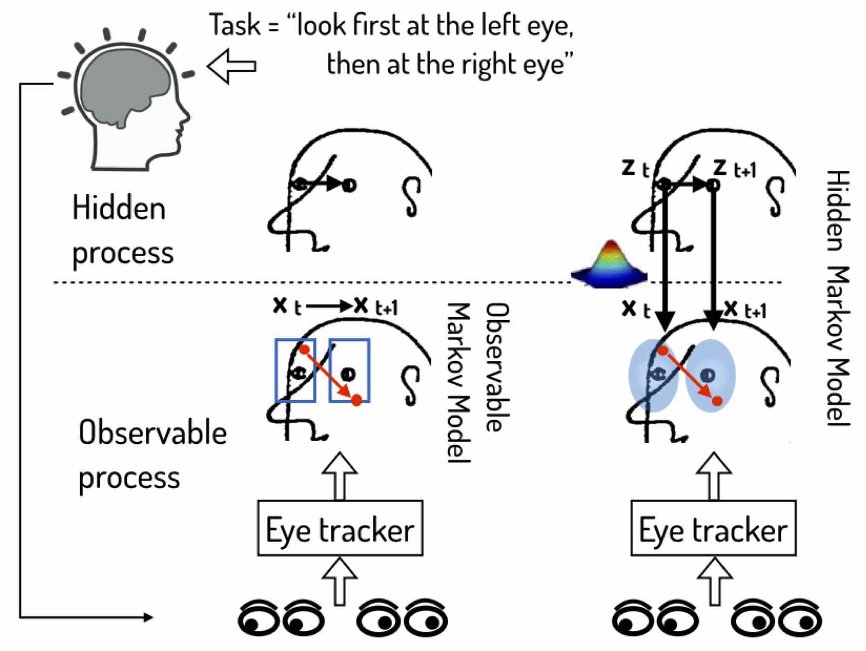
Figure 36: Observable Markov Model vs. HMM. We assume the task “look first at the left eye, then at the right eye” of Klee’s drawing presented in Fig. 17. The noise-free state space is here $S=\{s_{1}=\text{``left eye''},s_{2}=\text{``right eye''}\}$, where, ideally, $s_{1},s_{2}$ are exactly centred on the eyes. Thus, the “perfect shift” of the mind’s eye would be $\mathbf{z}_{t}=s_{1}\rightarrow\mathbf{z}_{t+1}=s_{2}$. However, as in Plato’s cave, we can only observe the noisy and variable eye-tracked shift $\mathbf{x}_{t},\rightarrow\mathbf{x}_{t+1}$ as a surrogate. The observable Markov Model simplifies the analysis by considering the two ROIs as a coarse-grained representation of the hidden states $s_{1},s_{2}$ and assumes all $\mathbf{x}_{t}$’s falling within the ROI as equivalent. On the contrary, the HMM allows the hidden shift $\mathbf{z}_{t}\rightarrow\mathbf{z}_{t+1}$ to be part of the model, and the visible shift $\mathbf{x}_{t}\rightarrow\mathbf{x}_{t+1}$ to be nothing but its sampled noisy realisation (e.g., Gaussian). See text for details.

As a more principled alternative (see, Fig. 36) one can assume that the exact points of interest, correspond to “hidden” targets or states: when, under a given task, one such target is chosen at time $t$, say $\mathbf{z}_{t}$, the corresponding actual fixation $\mathbf{x}_{t}$ will be generated by adding some noise $\epsilon$ (e.g., distributed according to a zero mean Gaussian pdf), i.e. $\mathbf{x}_{t}=\mathbf{z}_{t}+\epsilon$. In other terms, we are assuming that $P(\mathbf{x}_{t}\mid\mathbf{z}_{t})=\mathcal{N}(\mathbf{x}_{t};\mathbf{z}_{t},\Sigma)$. That is, when $\mathbf{z}_{t}$ is chosen, the actual observation is obtained by sampling from a Gaussian distribution $\mathcal{N}(\mathbf{x}_{t};\mathbf{z}_{t},\Sigma)$ centred on the true target $\mathbf{z}_{t}$, where the inverse of the covariance matrix $\Sigma$ will define the precision of target shooting.

t]

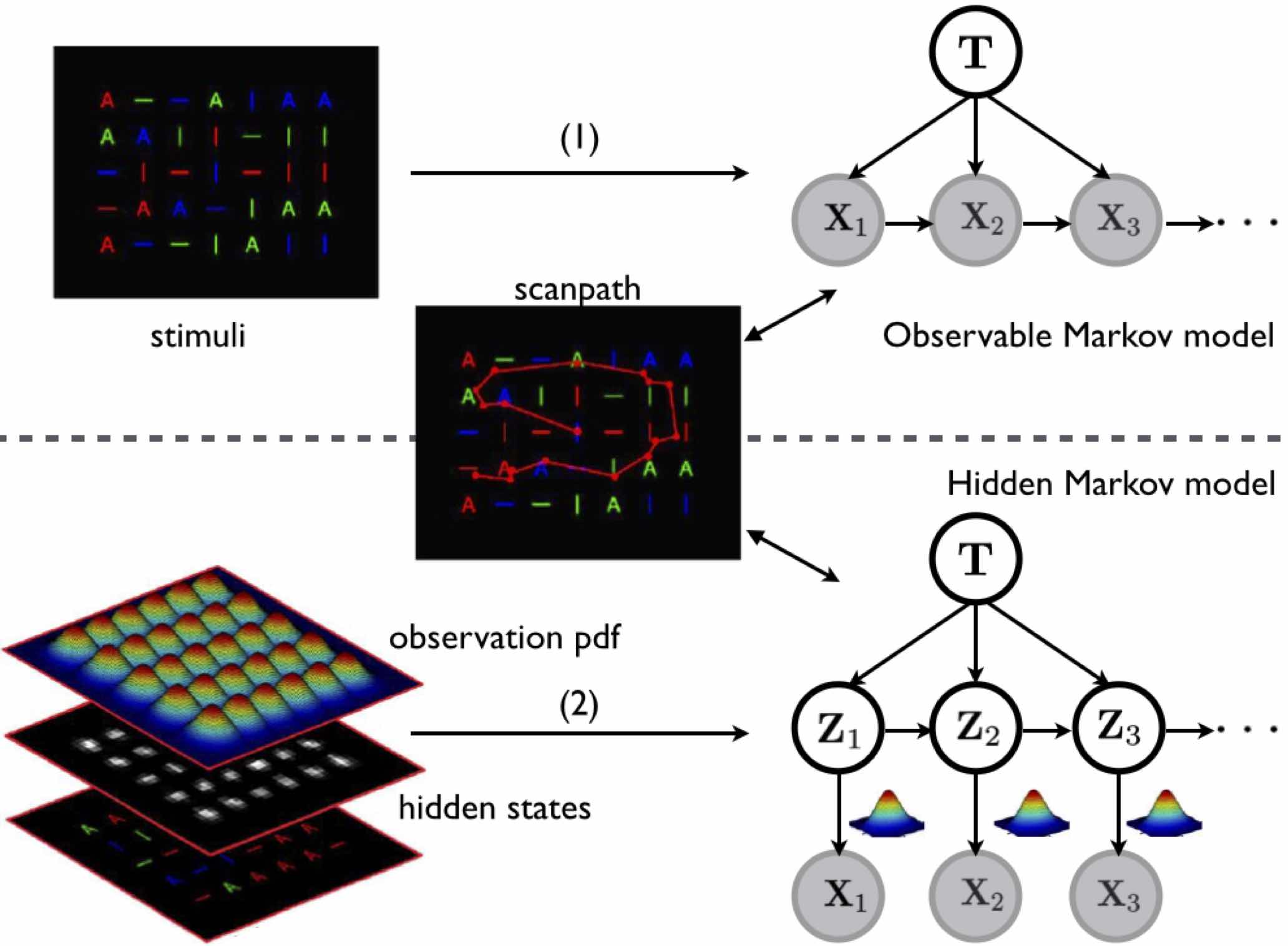
Figure 37: Two solutions for the inverse Yarbus given a time series of observations: (1) the task-conditioned observable Markov model hacisalihzade1992visual ; ellistark (top panel) and the task-conditioned hidden Markov model haji2013computational (bottom panel)

An HMM can be explicitly conditioned on task $\mathbf{T}$ generalising to the the Dynamic Bayesian Network depicted in Fig.  37 (bottom panel, solution $2$). The problem of learning such DBN can be further simplified by learning a separate HMM for a given task $\mathbf{T}=t_{k}$. This way each task will be implicitly defined through the set of parameters defining the corresponding HMM, $\mathbf{T}=t_{k}\Longleftrightarrow\Theta=\Theta_{k}$ (cfr, Fig. 38

Eventually, task inference is performed by choosing the HMM providing the higher likelihood for the input observation $\mathbf{x}_{new}$.

t]

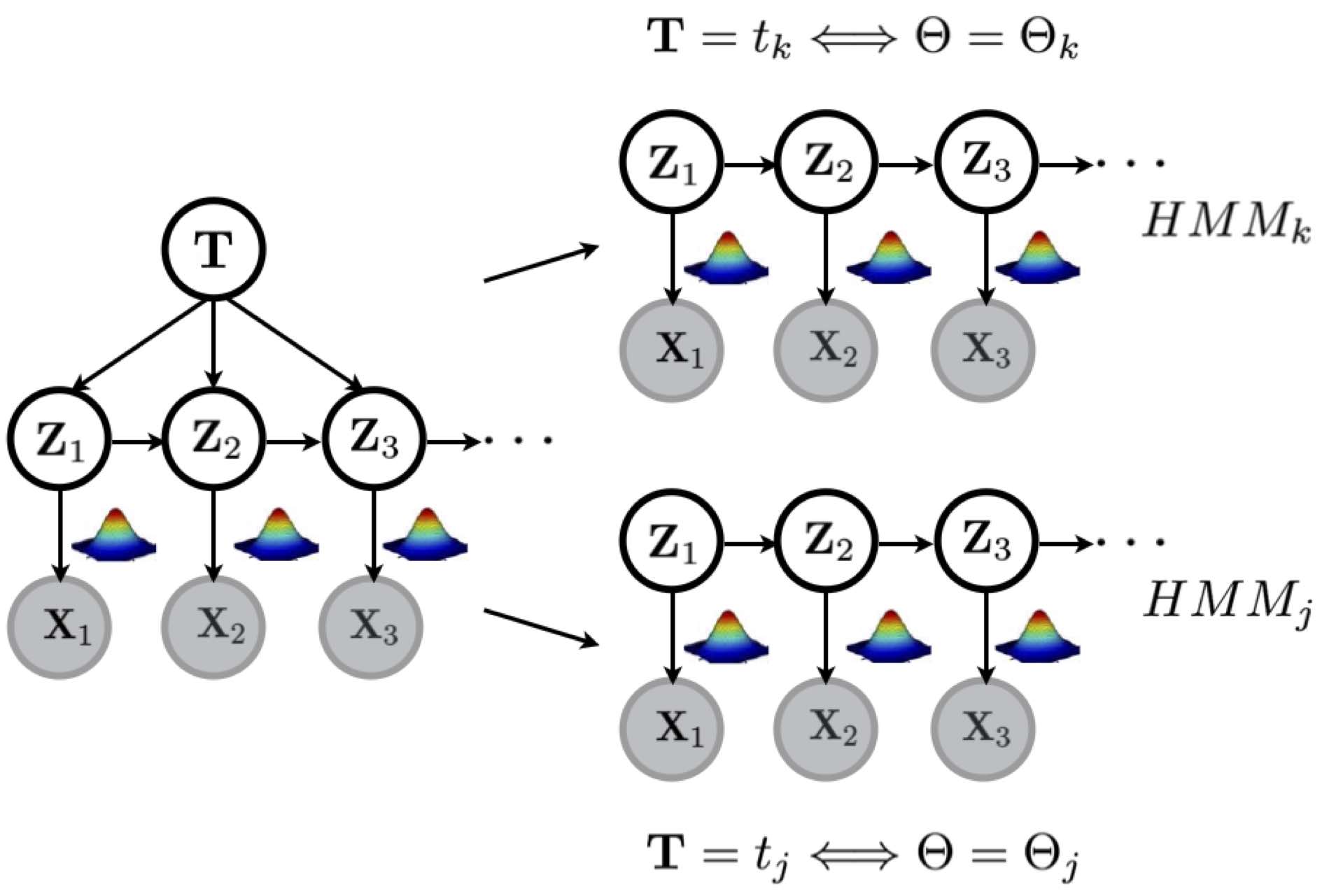
Figure 38: For $K$ tasks, the problem of learning the parameters for the DBN on the left is simplified to learning $K$ simple HMM parameters. In the learning stage, for each task $\mathbf{T}=t_{k}$ a specific set of parameter $\Theta_{k}$ is from observations, obtaining the $k$-th HMM. Task inference is performed by choosing the HMM providing the higher likelihood for the input observation $\mathbf{x}_{new}$

A nice study using HMM in the specific context of face exploration modelling has been presented by Coutrot et al. coutrot2016face . In this study, similarly to the example outlined in Fig. 36, each hidden state represents specific parts of the face that are likely to be fixated; the actual distribution of eye positions (emission density) is modelled as a 2-D Gaussian distribution. Coutrot et al. Coutrot2017 have recently a Matlab toolbox freely available to the community to support scan path modeling and classification with HMMs. A more complex example of how to exploit more general DBNs - namely, an Input-Output Coupled HMM - for dynamically intertwining eye movements and hand actions in a drawing task is provided in Coen-Cagli et al. coen2009visuomotor ; cagli2008draughtsman .

8.2 Assessing cognitive impairments and expertise

Eq. (110), can be used beyond the important issue of task classification. More generally, the value of $\mathbf{T}$ can represent a label $\ell$ to identify groups of observers that exhibit different eye movement behaviour with respect to a given task. In these circumstances, Eq. (110) formalises the probability that one observer belongs to one group. The posterior can then be used for classification (e.g., via the $\arg\max$ decision rule).

Case study: Assessing cognitive impairments

On the rationale that patients with mild cognitive impairment (MCI) often progress to Alzheimer’s disease (AD), Lagun et al. lagun2011detecting applied ML methods to analyse and exploit the information contained in the characteristics of eye movement exhibited by healthy and impaired subjects during the viewing of stimuli in the Visual Paired Comparison (VPC) task for the detection of memory impairment associated with MCI. The VPC assessment proceeds in two steps. During the familiarisation phase, subjects are presented with two identical visual stimuli, side by side, on a computer screen. Eye tracked subjects are allowed to look at the pictures for a specified amount of time. During the test phase, subjects are presented with pictures of the old stimulus and a novel stimulus, side by side. Control subjects typically spend $70\%$ of the time during the test phase looking at the novel stimulus, which indicates that they have a memory for the repeated, and now less interesting, stimulus. In contrast, age-matched MCI patients did not spend more time looking at the novel stimulus than the repeated stimulus.

Data analysis was conducted via supervised classification (two class/label problem, $\mathbf{T}$ taking values in $\ell=\{\text{``impaired''},\text{``control''}\}$), by exploiting standard techniques, namely Naïve Bayes, Logistic Regression, and the Support Vector Machine. They first trained the classification models on the multidimensional representation $\mathbf{X}$ of eye movements from a sample of the impaired and control subjects, $\mathcal{D}=\{\mathbf{x}_{train},\ell\}$ and then used the model to predict the status of new subjects based on their eye movement characteristics, i.e, $P(\mathbf{T}\mid\mathbf{X}=\mathbf{x}_{new})$. The results showed that eye movement characteristics including fixation duration, saccade length and direction, and re-fixation patterns (gaze position re-visits on previously seen parts of the stimuli) can be used to automatically distinguish impaired and normal subjects. In this study the SVM classifier outperformed the other techniques.

Beyond the specific issue addressed by Lagun et al., it is worth looking at their paper lagun2011detecting because it provides a gentle introduction to the Naïve Bayes, Logistic Regression, and SVM algorithms.

Case study: Classifying billiard player expertise

The study presented in boccignone_jemr2014 analysed the oculomotor behaviour of individual observers engaged in a visual task, with the aim of classifying them as experts or novices (two class/label problem, $\mathbf{T}$ taking values in $\ell=\{\text{``expert''},\text{``novice''}\}$). To this end, various visual stimuli and tasks were administered to $42$ subjects, half novices and half expert billiard players. Stimuli were a portion of a real match, video-recorded from the top, containing several shots of variable length and complexity, as well as a number of ad-hoc individual shots, also video-recorded from the top in a real setting. The match stimulus was associated to a free-viewing observation condition, while for the individual shots, which were occluded in the final part of the trajectory, observers were asked to predict the outcome of the shot, which placed implicitly a significant constraint on the deployment of visuospatial attention, and, consequently, on the overt scan path.

The input $\mathbf{X}$ was obtained as follows. For each observer, given the sequence of fixations $\{\mathbf{x}_{t}\}_{t=1}^{N_{T}}$, where the vector $\mathbf{x}_{t}$ represents the fixation position (coordinates) at time $t$, the amplitude and direction of each gaze shift were computed: $\{l_{t},\theta_{t}\}_{t=1}$. Third feature was the fixation duration $\{f_{t}\}_{t=1}^{N_{T}}$.

The random sample $\{l_{t},\theta_{t},f_{t}\}_{t=1}^{N_{T}}$ was summarised through the empirical distribution functions (histograms), that is the random vectors $\mathbf{x}^{l}=\left[x^{l}_{1}\cdots x^{l}_{D}\right]^{T}$, $\mathbf{x}^{\theta}=\left[x^{\theta}_{1}\cdots x^{\theta}_{D}\right]^{T}$ and $\mathbf{x}^{f}=\left[x^{f}_{1}\cdots x^{f}_{D}\right]^{T}$, respectively, where the vector dimension $D$ represents the number of bins of the histogram. The feature vector $\mathbf{x}^{s}$ is thus a summary of the behaviour of a single observer with respect to a particular feature space or source of information $s=1,\dots S$, here $S=3$. Thus, eventually, $\mathbf{X}=\{\mathbf{x}^{s}\}_{s=1}^{S}$.

t]

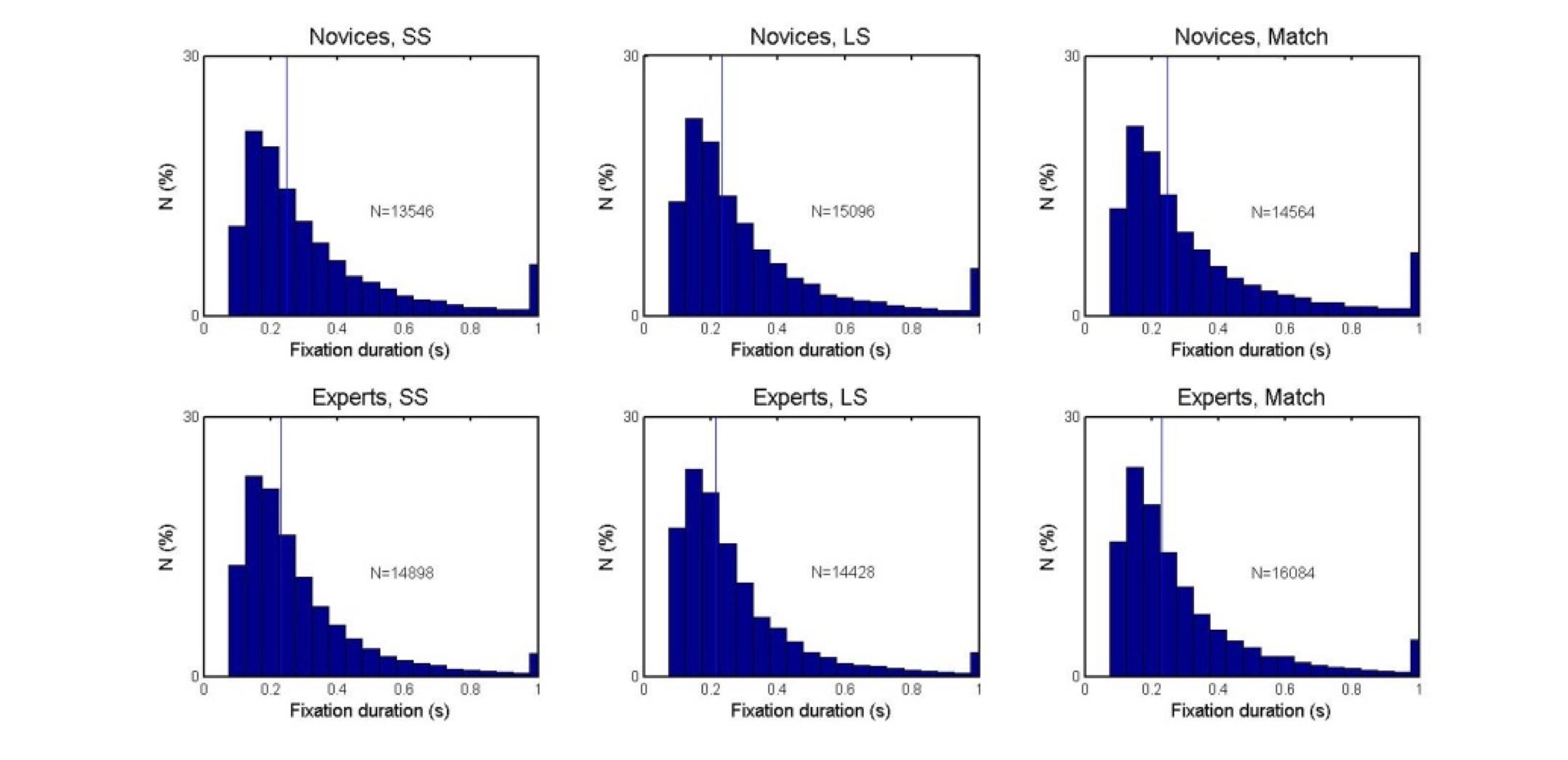
(a) Fixation duration

(b) Gaze shift amplitude

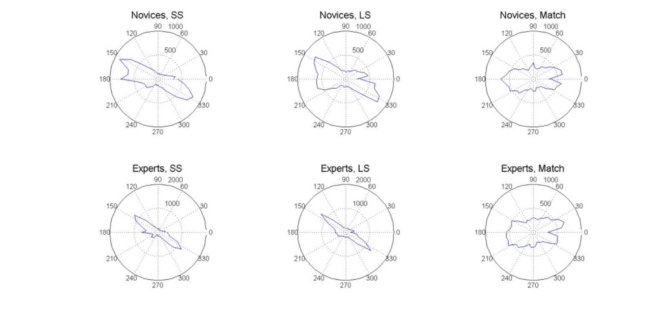
(c) Gaze shift direction

Figure 39: Empirical distributions (histograms) of $\{l_{t},\theta_{t},f_{t}\}_{t=1}^{N_{T}}$ used to classify expertise. Top panels (39(a)), fixation duration; middle panels (39(b)), gaze shift amplitude; bottom panels (39(c)), gaze shift direction. Vertical solid lines, median values. SS=Short Shots, LS=Long Shots. Modified after boccignone_jemr2014

From Fig. 39, note that differences between experts and novices are barely noticeable in terms of features. Clearly, when addressing a scenario in which individual observers are classified as belonging to one or another population, and differences between features are so subtle, more sophisticated ML tools are needed. On this basis, each feature space $s$ was treated as independent and mapped to a specific kernel space (either linear or Gaussian, murphy2012machine ). Then, the posterior $P(\mathbf{T}\mid\mathbf{X})$ was rewritten as $P(t_{n}|\mathbf{x}_{n}^{1},...,\mathbf{x}_{n}^{S})=P(t_{n}|\mathbf{W},\mathbf{k}^{\beta}_{n})$, where the term on the r.h.s is the Multinomial probit likelihood. Here, $\mathbf{W}\in\mathbb{R}^{N\times C}$ is the matrix of model parameters; the variable $\mathbf{k}^{\beta}_{n}$ is a row of the kernel matrix $\mathbf{K}^{\beta}\in\mathbb{R}^{N\times N}$ - whose elements are the $K^{\beta}(\mathbf{x}_{i},\mathbf{x}_{j})$, i.e. the different kernels - and it expresses how related, based on the selected kernel function, observation $\mathbf{x}_{n}$ is to the others of the training set. This way (cfr. Fig. 40), sources can be combined within a composite kernel space level and classified through a Relevance Vector Machine (RVM), namely a multiple-kernel RVM psorakis2010multiclass ; damoulas2009combining .

t]

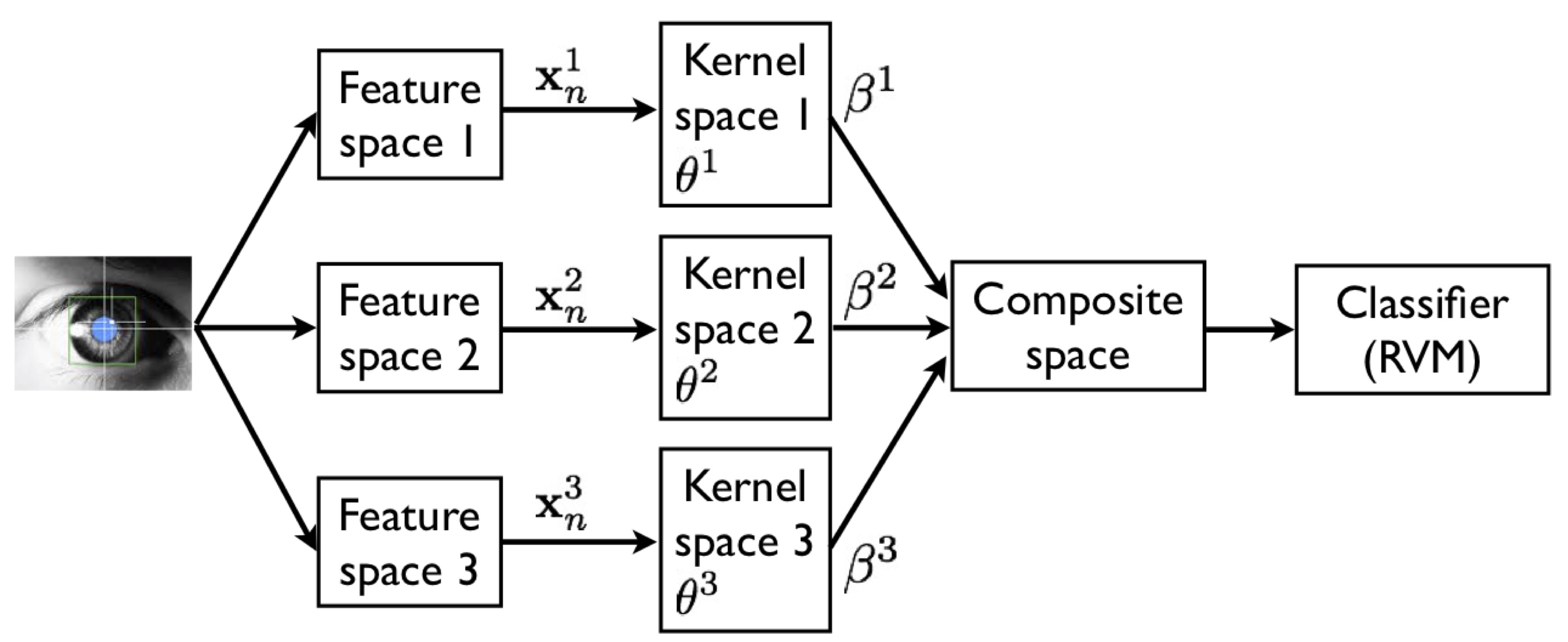
Figure 40: Data analysis in multiple-kernel representation. The fixation sequence is represented in different feature spaces $s=1,\cdots,S$; each feature $\mathbf{x}^{s}$ is then separately mapped in a kernel space, each space being generated via kernel $K^{s}$ of parameters $\theta^{s}$. The separate kernel spaces are then combined in a composite kernel space, which is eventually used for classification. Modified after boccignone_jemr2014

Discussing in detail this solution is out of the scope of this chapter (see boccignone_jemr2014 of a short presentation, and Bishop BishopPRML for more details). However, just to give some hints, RVMs can be considered the Bayesian counterpart of SVMs. They are Bayesian sparse machines, that is they employ sparse Bayesian learning via an appropriate prior formulation. Not only do they overcome some of the limitations affecting SVMs but also they achieve sparser solutions (and hence they are faster at test time) than SVM. Indeed, by combining only three basic parameters of visual exploration, the overall classification accuracy, expressed as percent correct and averaged across stimulus types and oculomotor features, scored a respectable $78\%$. More interesting is to consider the best performance for each stimulus type, which testifies the achievement of the classifier, and which depends on the features used. The best performance ranged between $81.90\%$ and $88.09\%$ - $1.852$ to $2.399$ in terms of $d^{{}^{\prime}}$, which is an interesting result, especially considering the naturalistic, unconstrained viewing condition.

9 A final note on the use of Machine Learning in visual attention modelling

For the sake of completeness, it is worth mentioning that modern Statistical Machine Learning techniques such as those described in the previous Section, are currently adopted even at the earliest stages of visual attention modelling, markedly in salience computation.

Going back to Eqs. 14 and 15 (Section 4), as we already pointed out, in the case the prior $P(\mathbf{L})$ is assumed to be uniform (no spatial bias, no preferred locations), then $P(\mathbf{L}=1\mid\mathbf{F})\simeq P(\mathbf{F}\mid\mathbf{L}=1)$, where $\mathbf{L}=1$ is now a binary RV ($1$ or $0$) simply denoting location $(x,y)$ as salient/non salient. In such case, the likelihood function $P(\mathbf{F}\mid\mathbf{L}=1)$ can be determined in many ways; e.g., nonparametric kernel density estimation has been addressed seo2009 , where center / surround local regression kernels are exploited for computing $\mathbf{F}$.

More generally, taking into account the ratio $f(\mathbf{L})=\frac{P(\mathbf{L}=1\mid\mathbf{F})}{P(\mathbf{L}=0\mid\mathbf{F})}$ (or, commonly, the log-ratio) casts the saliency detection problem in a classification problem, in particular a discriminative one, for which a variety of learning techniques are readily available. Kienzle and colleagues kienzle2006nonparametric pioneered this approach by learning the saliency discriminant function $f(\mathbf{L})$ directly from human eye tracking data using an SVM. Their approach has paved the way to a relevant number of works: from judd2009learning – where a linear SVM is trained from human fixation data using a set of low, middle and high-level features to define salient locations–, to most recent ones that wholeheartedly endorse ML trends. Henceforth, methods have been proposed relying on sparse representation of “feature words” (atoms) encoded in salient and non-salient dictionaries; these are either learned from local image patches yan2010visual ; lang2012saliency or from eye tracking data of training images jiang2015image . Graph-based learning is one other trend, from the seminal work of Harel et al. harel2007graph to yu2014maximal (see the latter, for a brief review of this field). Crucially, for the research practice, data-driven learning methods allow to contend with large scale dynamic datasets. SVMs are used by Mathe and Sminchisescu mathe2015actions in the vein of kienzle2006nonparametric and judd2009learning , but they remarkably exploit state-of-the art computer vision datasets annotated with human eye movements collected under the ecological constraints of a visual action recognition task.

As a general comment on (discriminative) ML-based methods, on the one hand it is embraceable the criticism by Borji and Itti BorItti2012 , who surmise that these techniques make “models data-dependent, thus influencing fair model comparison, slow, and to some extent, black-box.” But on the other hand, one important lesson of these approaches lies in that they provides a data-driven way of deriving the most relevant visual features as optimal predictors. The learned patterns can shape receptive fields (filters) that have equivalent or superior predictive power when compared against hand-crafted (and sometimes more complicated) models kienzle2009center . Certainly, this lesson is at the base of the current exponentially growth of methods based on deep learning techniques lecun2015deep , in particular Convolutional Neural Networks (CNN, cfr. deepTaxonomy2016 for a focused review), where the computed features seem to outperform, at least from an engineering perspective, most of, if not all, the state-of-the art features conceived in computer vision.

Again, CNNs, as commonly exploited in the current practice, bring no significant conceptual novelty as to the use of Eq. 14: fixation prediction is formulated as a supervised binary classification problem (in some case, regression is addressed, wang2016deep ). For example, in vig2014large a linear SVM is used for learning the saliency discriminant function $f(\mathbf{L})$ after a large-scale search for optimal features $\mathbf{F}$. Similarly, Shen et al. shenZhao2014learning detect salient region via linear SVM fed with features computed from multi-layer sparse network model. Work described in lin2014saliency uses the simple normalization step IttiKoch98 to approximate $P(\mathbf{L}=1\mid\mathbf{F})$, where in kruthiventi2015deepfix the last $1\times 1$ convolutional layer of a fully convolutional net is exploited. Cogent here is the outstanding performance of CNN in learning and representing features that correlate well with eye fixations, like objects, faces, context.

Clearly, one problem is the enormous amount of training data necessary to train these networks, and the engineering expertise required, which makes them difficult to apply for predicting saliency. However, Kümmerer et al. kummerer2014deep by exploiting the well known network from AlexNetNIPS2012 as starting point, have given evidence that deep CNN trained on computer vision tasks like object detection boost saliency prediction. The network described in AlexNetNIPS2012 has been optimised for object recognition using a massive dataset consisting of more than one million images, and results reported kummerer2014deep on static pictures are impressive when compared to state-of-the-art methods, even to previous CNN-based proposals vig2014large .

10 Suggested readings

To explore beyond the contents of this Chapter, we recommend the following. A brief and clear introduction to stochastic processes (from a physicist’s point of view) can be found in a few chapters of Huang’s “Introduction to statistical physics” huang2001introduction . A comprehensive treatment of stochastic processes is given in Gardiner’s “Stochastic Methods: A Handbook for the Natural and Social Sciences” gardiner2009stochastic ; it is a great starting point if you are looking for specific information about a specific stochastic process. One of the finest books on stochastic processes is van Kampen’s classic “Stochastic processes in physics and chemistry” vankampen ; difficult reading, but well–worth the effort. A modern treatment of the subject is provided in Paul and Baschnagel “Stochastic Processes – From Physics to Finance” paul2013stochastic , with a clear discussion of what happens beyond the Central Limit Theorem.

A beautiful bridge between stochastic processes and foraging is outlined in Méndez, Campos, and Bartumeus, “Stochastic Foundations in Movement Ecology: Anomalous Diffusion, Front Propagation and Random Searches” mendez2014stochastic . However, if one wants to skip more technical details, an affordable, easy to read introduction to foraging and Lévy flights is “The physics of foraging” by Viswanathan et al. viswanathan2011physics .

Eventually, for what concerns Statistical Machine Learning, which is nowadays a vast field, a thorough and simple introduction is provided by Rogers and Girolami rogers2011first . A deeper insight can be gained by reading Bishop’s textbook BishopPRML . The most comprehensive and up-to-date textbook is that by Kevin Murphy murphy2012machine . If some of the readers are daring to surf the big wave of deep learning, then the book by Goodfellow, Bengio and Courville Goodfellow-et-al-2016 provides the vital outfit.

11 Questions students should be able to answer

1. What are the main reasons for considering the sequence of gaze shifts to be the observable outcome of a stochastic process?

2. If you were to set up a probabilistic model of gaze shifts, which factors would you consider to design a prior distribution $P(\mathbf{x})$ on gaze position $\mathbf{x}$?

3. What kind of information is provided by a Probabilistic Graphical Model?

4. You have conducted an eye tracking experiment where you recorded the first ten fixations for each subject, say $\mathbf{x}_{i}$, $i=1,2,\cdots,10$ at times $t_{i}$, $i=1,2,\cdots,10$. You devise two possible models:

   $$P(\mathbf{x}_{1},t_{1};\mathbf{x}_{2},t_{2};\cdots)=\prod_{i=1}^{10}P(\mathbf{x}_{i},t_{i}),$$

   $$P(\mathbf{x}_{1},t_{1};\mathbf{x}_{2},t_{2};\cdots)=P(\mathbf{x}_{1},t_{1})\prod_{i=2}^{10}P(\mathbf{x}_{i},t_{i}\mid\mathbf{x}_{i-1},t_{i-1}).$$

   What are the assumptions behind the two models? What are the pros and cons of each model?

5. You set up an eye tracking experiment where a control group and a patient group observe pictures displaying a number of objects of interest. At the end of the experiment you define objects as Areas of Interest (AOIs) and compute the observation transition frequency between AOIs in each picture for each subject of the two groups. What is the probabilistic model behind such statistics?

6. You are simulating a 2-dimensional stochastic process according to the following equations:

   $$x_{t}=\xi_{x,t}$$

   $$y_{t}=\xi_{y,t},$$

   where $x_{t},y_{t}$ denote spatial coordinates and the random variable $\xi_{x,t}$ is sampled from a $1$-dimensional Gaussian distribution $\mathcal{N}(\mu_{x},\sigma^{2})$, i.e. $\xi_{x,t}\sim\mathcal{N}(\mu,\sigma^{2})$, with $\mu_{x}=10,\sigma=1$, while $\xi_{y,t}\sim\mathcal{N}(\mu_{y},\sigma^{2})$, with $\mu_{y}=10$. What kind of $2$-dimensional pattern is likely to be drawn if you run the simulation for $t=1,2,\cdots 100$ iterations?

7. You are studying the central fixation bias in scene viewing (i.e., the marked tendency to fixate the center of the screen when viewing scenes on computer monitors). The resolution of the CRT monitor where stimuli are presented is $1280\times 1020$ pixels. What could be a possible microscopic level description of such bias? What a possible macroscopic description? (Hint: Reconsider Question 5)

8. Assume that you are able to fit the empirical distribution of some experimental data with the law $P(x)\approx x^{-\mu}$. Which kind of information cold you infer from such result?

9. Repeat the simulation proposed in Question 5, but now assume to sample $\xi_{x,t}$ and $\xi_{y,t}$ from a Cauchy distribution $\frac{1}{\pi\gamma}\left[\frac{\gamma^{2}}{(\xi-\delta)^{2}+\gamma^{2}}\right]$ with $\delta=10$, $\gamma=1$. What kind of $2$-dimensional pattern do you expect? Would the histogram of the sequence of step amplitudes have a bell shape? Could we still consider this kind of random walk a Markovian walk?

10. You plan an eye tracking experiment with $n$ subjects to distinguish experts from non experts when viewing five paintings. After recording the data, you define a number $N_{k}$ of AOIs on paintings (for simplicity, assume an equal number for all paintings). Then, for each subject and each painting, you measure $l_{k}$ and $t_{k}$, namely the number of fixations and the average fixation time, respectively, in $k$-th AOI, $k=1,2,\cdots,N_{k}$. How would you proceed to make the desired discrimination?

References

- (1) Aks, D.J., Zelinsky, G.J., Sprott, J.C.: Memory across eye-movements: 1/f dynamic in visual search. Nonlinear dynamics, psychology, and life sciences 6(1), 1–25 (2002)
- (2) Bachelier, L.: Théorie de la spéculation. Gauthier-Villars (1900)
- (3) Barber, D., Cemgil, A.T., Chiappa, S.: Bayesian time series models. Cambridge University Press (2011)
- (4) Baronchelli, A., Radicchi, F.: Lévy flights in human behavior and cognition. Chaos, Solitons & Fractals 56, 101–105 (2013)
- (5) Begum, M., Karray, F., Mann, G., Gosine, R.: A probabilistic model of overt visual attention for cognitive robots. Systems, Man, and Cybernetics, Part B: Cybernetics, IEEE Transactions on 40(5), 1305–1318 (2010)
- (6) Bishop, C.M.: Pattern Recognition and Machine Learning (Information Science and Statistics). Springer-Verlag New York, Inc., Secaucus, NJ, USA (2006)
- (7) Boccignone, G., Ferraro, M.: Modelling gaze shift as a constrained random walk. Physica A: Statistical Mechanics and its Applications 331(1-2), 207–218 (2004)
- (8) Boccignone, G., Ferraro, M.: The active sampling of gaze-shifts. In: G. Maino, G. Foresti (eds.) Image Analysis and Processing ICIAP 2011, Lecture Notes in Computer Science, vol. 6978, pp. 187–196. Springer Berlin / Heidelberg (2011)
- (9) Boccignone, G., Ferraro, M.: Feed and fly control of visual scanpaths for foveation image processing. annals of telecommunications-annales des télécommunications 68(3-4), 201–217 (2013)
- (10) Boccignone, G., Ferraro, M.: Gaze shift behavior on video as composite information foraging. Signal Processing: Image Communication 28(8), 949 – 966 (2013)
- (11) Boccignone, G., Ferraro, M.: Ecological sampling of gaze shifts. IEEE Trans. on Cybernetics 44(2), 266–279 (2014)
- (12) Boccignone, G., Ferraro, M., Caelli, T.: An information-theoretic approach to active vision. In: Proceedings 11th International Conference on Image Analysis and Processing, (ICIAP), pp. 340–345. IEEE Press (2001)
- (13) Boccignone, G., Ferraro, M., Crespi, S., Robino, C., de’Sperati, C.: Detecting expert’s eye using a multiple-kernel relevance vector machine. Journal of eye movement research 7(2), 1–15 (2014)
- (14) Boccignone, G., Marcelli, A., Napoletano, P., Di Fiore, G., Iacovoni, G., Morsa, S.: Bayesian integration of face and low-level cues for foveated video coding. IEEE Transactions on Circuits and Systems for Video Technology 18(12), 1727–1740 (2008)
- (15) Borji, A., Itti, L.: State-of-the-art in visual attention modeling. IEEE Transactions on Pattern Analysis and Machine Intelligence 35(1), 185–207 (2013)
- (16) Borji, A., Sihite, D.N., Itti, L.: An object-based bayesian framework for top-down visual attention. In: Twenty-Sixth AAAI Conference on Artificial Intelligence (2012)
- (17) Brockmann, D., Geisel, T.: The ecology of gaze shifts. Neurocomputing 32(1), 643–650 (2000)
- (18) Bundesen, C.: A computational theory of visual attention. Philosophical Transactions of the Royal Society of London. Series B: Biological Sciences 353(1373), 1271–1281 (1998)
- (19) Cain, M.S., Vul, E., Clark, K., Mitroff, S.R.: A bayesian optimal foraging model of human visual search. Psychological science 23(9), 1047–1054 (2012)
- (20) Canosa, R.: Real-world vision: Selective perception and task. ACM Transactions on Applied Perception 6(2), 11 (2009)
- (21) Carpenter, R., Williams, M.: Neural computation of log likelihood in control of saccadic eye movements. Nature 377(6544), 59–62 (1995)
- (22) Cerf, M., Frady, E., Koch, C.: Faces and text attract gaze independent of the task: Experimental data and computer model. Journal of Vision 9(12) (2009)
- (23) Cerf, M., Harel, J., Einhäuser, W., Koch, C.: Predicting human gaze using low-level saliency combined with face detection. Advances in neural information processing systems 20 (2008)
- (24) Chambers, J., Mallows, C., Stuck, B.: A method for simulating stable random variables. J. Am. Stat. Ass. 71(354), 340–344 (1976)
- (25) Chernyak, D.A., Stark, L.W.: Top–down guided eye movements. IEEE Trans. Systems Man Cybernetics - B 31, 514–522 (2001)
- (26) Chikkerur, S., Serre, T., Tan, C., Poggio, T.: What and where: A bayesian inference theory of attention. Vision research 50(22), 2233–2247 (2010)
- (27) Clavelli, A., Karatzas, D., Lladós, J., Ferraro, M., Boccignone, G.: Modelling task-dependent eye guidance to objects in pictures. Cognitive Computation 6(3), 558–584 (2014)
- (28) Codling, E., Plank, M., Benhamou, S.: Random walk models in biology. Journal of the Royal Society Interface 5(25), 813 (2008)
- (29) Coen-Cagli, R., Coraggio, P., Napoletano, P., Boccignone, G.: What the draughtsman’s hand tells the draughtsman’s eye: A sensorimotor account of drawing. International Journal of Pattern Recognition and Artificial Intelligence 22(05), 1015–1029 (2008)
- (30) Coen-Cagli, R., Coraggio, P., Napoletano, P., Schwartz, O., Ferraro, M., Boccignone, G.: Visuomotor characterization of eye movements in a drawing task. Vision research 49(8), 810–818 (2009)
- (31) Costa, T., Boccignone, G., Cauda, F., Ferraro, M.: The foraging brain: evidence of levy dynamics in brain networks. PloS one 11(9), e0161,702 (2016)
- (32) Coutrot, A., Binetti, N., Harrison, C., Mareschal, I., Johnston, A.: Face exploration dynamics differentiate men and women. Journal of Vision 16(14), 16–16 (2016)
- (33) Coutrot, A., Hsiao, J.H., Chan, A.B.: Scanpath modeling and classification with hidden markov models. Behavior Research Methods (2017). URL https://doi.org/10.3758/s13428-017-0876-8
- (34) Cowpertwait, P.S., Metcalfe, A.V.: Introductory time series with R. Springer, Dordrecht (2009)
- (35) Damoulas, T., Girolami, M.A.: Combining feature spaces for classification. Pattern Recognition 42(11), 2671–2683 (2009)
- (36) deCroon, G., Postma, E., van den Herik, H.J.: Adaptive Gaze Control for Object Detection. Cognitive Computation 3, 264–278 (2011)
- (37) Desimone, R., Duncan, J.: Neural mechanisms of selective visual attention. Annual review of neuroscience 18(1), 193–222 (1995)
- (38) Doob, J.L.: The brownian movement and stochastic equations. Annals of Mathematics pp. 351–369 (1942)
- (39) Dorr, M., Martinetz, T., Gegenfurtner, K., Barth, E.: Variability of eye movements when viewing dynamic natural scenes. Journal of Vision 10(10) (2010)
- (40) Dubkov, A.A., Spagnolo, B., Uchaikin, V.V.: Lévy flight superdiffusion: an introduction. International Journal of Bifurcation and Chaos 18(09), 2649–2672 (2008)
- (41) Einhäuser, W., Spain, M., Perona, P.: Objects predict fixations better than early saliency. Journal of Vision 8(14) (2008). DOI 10.1167/8.14.18. URL http://www.journalofvision.org/content/8/14/18.abstract
- (42) Einstein, A.: On the motion required by the molecular kinetic theory of heat of small particles suspended in a stationary liquid. Annalen der Physik 17, 549–560 (1905)
- (43) Einstein, A.: Zur theorie der brownschen bewegung. Annalen der Physik 324(2), 371–381 (1906)
- (44) Elazary, L., Itti, L.: A bayesian model for efficient visual search and recognition. Vision research 50(14), 1338–1352 (2010)
- (45) Ellis, S., Stark, L.: Statistical dependency in visual scanning. Human Factors: The Journal of the Human Factors and Ergonomics Society 28(4), 421–438 (1986)
- (46) Engbert, R.: Microsaccades: A microcosm for research on oculomotor control, attention, and visual perception. Progress in brain research 154, 177–192 (2006)
- (47) Engbert, R., Mergenthaler, K., Sinn, P., Pikovsky, A.: An integrated model of fixational eye movements and microsaccades. Proceedings of the National Academy of Sciences 108(39), E765–E770 (2011)
- (48) Feng, G.: Eye movements as time-series random variables: A stochastic model of eye movement control in reading. Cognitive Systems Research 7(1), 70–95 (2006)
- (49) Foulsham, T., Underwood, G.: What can saliency models predict about eye movements? spatial and sequential aspects of fixations during encoding and recognition. Journal of Vision 8(2) (2008)
- (50) Frintrop, S., Rome, E., Christensen, H.: Computational visual attention systems and their cognitive foundations: A survey. ACM Trans. on Applied Perception 7(1), 6 (2010)
- (51) Gardiner, C.: Stochastic Methods: A Handbook for the Natural and Social Sciences. Springer Series in Synergetics. Springer-Verlag, Berlin, Heidelberg (2009)
- (52) Gnedenko, B., Kolmogórov, A.: Limit distributions for sums of independent random variables. Addison-Wesley Pub. Co. (1954)
- (53) Goodfellow, I., Bengio, Y., Courville, A.: Deep Learning. MIT Press (2016). http://www.deeplearningbook.org
- (54) Hacisalihzade, S., Stark, L., Allen, J.: Visual perception and sequences of eye movement fixations: A stochastic modeling approach. IEEE Trans. Syst., Man, Cybern. 22(3), 474–481 (1992)
- (55) Haji-Abolhassani, A., Clark, J.J.: A computational model for task inference in visual search. Journal of vision 13(3), 29 (2013)
- (56) Harel, J., Koch, C., Perona, P.: Graph-based visual saliency. In: Advances in neural information processing systems, vol. 19, pp. 545–552. MIT Press, Cambridge, MA (2007)
- (57) Heinke, D., Backhaus, A.: Modelling visual search with the selective attention for identification model (vs-saim): a novel explanation for visual search asymmetries. Cognitive computation 3(1), 185–205 (2011)
- (58) Heinke, D., Humphreys, G.W.: Attention, spatial representation, and visual neglect: simulating emergent attention and spatial memory in the selective attention for identification model (saim). Psychological review 110(1), 29 (2003)
- (59) Heinke, D., Humphreys, G.W.: Computational models of visual selective attention: A review. Connectionist models in cognitive psychology 1(4), 273–312 (2005)
- (60) Henderson, J.M., Shinkareva, S.V., Wang, J., Luke, S.G., Olejarczyk, J.: Predicting cognitive state from eye movements. PLoS ONE 8(5), e64,937 (2013)
- (61) Higham, D.: An algorithmic introduction to numerical simulation of stochastic differential equations. SIAM review pp. 525–546 (2001)
- (62) Hills, T.T.: Animal foraging and the evolution of goal-directed cognition. Cognitive Science 30(1), 3–41 (2006)
- (63) Ho Phuoc, T., Guérin-Dugué, A., Guyader, N.: A computational saliency model integrating saccade programming. In: Proc. Int. Conf. on Bio-inspired Systems and Signal Processing, pp. 57–64. Porto, Portugal (2009)
- (64) Horowitz, T., Wolfe, J.: Visual search has no memory. Nature 394(6693), 575–577 (1998)
- (65) Huang, K.: Introduction to statistical physics. CRC Press, Boca Raton, FL (2001)
- (66) Humphreys, G.W., Muller, H.J.: Search via recursive rejection (serr): A connectionist model of visual search. Cognitive Psychology 25(1), 43–110 (1993)
- (67) Insua, D., Ruggeri, F., Wiper, M.: Bayesian analysis of stochastic process models. John Wiley & Sons (2012)
- (68) Itti, L., Koch, C., Niebur, E.: A model of saliency-based visual attention for rapid scene analysis. IEEE Transactions on Pattern Analysis and Machine Intelligence 20, 1254–1259 (1998)
- (69) Jarrow, R., Protter, P.: A short history of stochastic integration and mathematical finance: the early years, 1880-1970. Lecture Notes-Monograph Series pp. 75–91 (2004)
- (70) Jaynes, E.T.: Probability theory: the logic of science. Cambridge University Press, New York , NY (2003)
- (71) Jetley, S., Murray, N., Vig, E.: End-to-end saliency mapping via probability distribution prediction. In: Proceedings of the IEEE Conference on Computer Vision and Pattern Recognition, pp. 5753–5761 (2016)
- (72) Jiang, L., Xu, M., Ye, Z., Wang, Z.: Image saliency detection with sparse representation of learnt texture atoms. In: Proceedings of the IEEE International Conference on Computer Vision Workshops, pp. 54–62 (2015)
- (73) Judd, T., Ehinger, K., Durand, F., Torralba, A.: Learning to predict where humans look. In: IEEE 12th International conference on Computer Vision, pp. 2106–2113. IEEE (2009)
- (74) Keech, T., Resca, L.: Eye movements in active visual search: A computable phenomenological model. Attention, Perception, & Psychophysics 72(2), 285–307 (2010)
- (75) Kienzle, W., Franz, M.O., Schölkopf, B., Wichmann, F.A.: Center-surround patterns emerge as optimal predictors for human saccade targets. Journal of vision 9(5), 7–7 (2009)
- (76) Kienzle, W., Wichmann, F.A., Franz, M.O., Schölkopf, B.: A nonparametric approach to bottom-up visual saliency. In: Advances in neural information processing systems, pp. 689–696 (2006)
- (77) Kimura, A., Pang, D., Takeuchi, T., Yamato, J., Kashino, K.: Dynamic markov random fields for stochastic modeling of visual attention. In: Proc. ICPR ’08., pp. 1–5. IEEE (2008)
- (78) Koch, C., Ullman, S.: Shifts in selective visual attention: towards the underlying neural circuitry. Human Neurobiology 4(4), 219–27 (1985)
- (79) Koller, D., Friedman, N.: Probabilistic graphical models: principles and techniques. MIT press, Cambridge, MA (2009)
- (80) Kolmogorov, A., Gnedenko, B.: Limit distributions for sums of independent random variables. Addison-Wesley, Cambridge, Mass (1954)
- (81) Kolmogorov, A.N.: Dissipation of energy in isotropic turbulence. In: Dokl. Akad. Nauk SSSR, vol. 32, pp. 325–327 (1941)
- (82) Koutrouvelis, I.: Regression-type estimation of the parameters of stable laws. Journal of the American Statistical Association pp. 918–928 (1980)
- (83) Krizhevsky, A., Sutskever, I., Hinton, G.E.: Imagenet classification with deep convolutional neural networks. In: F. Pereira, C.J.C. Burges, L. Bottou, K.Q. Weinberger (eds.) Advances in Neural Information Processing Systems 25, pp. 1097–1105. Curran Associates, Inc. (2012)
- (84) Kruthiventi, S.S., Ayush, K., Babu, R.V.: Deepfix: A fully convolutional neural network for predicting human eye fixations. arXiv preprint arXiv:1510.02927 (2015)
- (85) Kümmerer, M., Theis, L., Bethge, M.: Deep gaze i: Boosting saliency prediction with feature maps trained on imagenet. arXiv preprint arXiv:1411.1045 (2014)
- (86) Lagun, D., Manzanares, C., Zola, S.M., Buffalo, E.A., Agichtein, E.: Detecting cognitive impairment by eye movement analysis using automatic classification algorithms. Journal of Neuroscience Methods 201(1), 196–203 (2011)
- (87) Laing, C., Lord, G.J.: Stochastic methods in neuroscience. Oxford University Press (2010)
- (88) Lang, C., Liu, G., Yu, J., Yan, S.: Saliency detection by multitask sparsity pursuit. IEEE Transactions on Image Processing 21(3), 1327–1338 (2012)
- (89) Langevin, P.: Sur la théorie du mouvement brownien. Comptes-Rendus Acad. Sci. Paris 146(530-533), 530 (1908)
- (90) Le Meur, O., Coutrot, A.: Introducing context-dependent and spatially-variant viewing biases in saccadic models. Vision Research 121, 72–84 (2016)
- (91) LeCun, Y., Bengio, Y., Hinton, G.: Deep learning. Nature 521(7553), 436–444 (2015)
- (92) Liberati, A., Fadda, R., Doneddu, G., Congiu, S., Javarone, M.A., Striano, T., Chessa, A.: A statistical physics perspective to understand social visual attention in autism spectrum disorder. Perception 46(8), 889–913 (2017)
- (93) Lin, Y., Kong, S., Wang, D., Zhuang, Y.: Saliency detection within a deep convolutional architecture. In: Workshops at the Twenty-Eighth AAAI Conference on Artificial Intelligence (2014)
- (94) Logan, G.D.: The code theory of visual attention: an integration of space-based and object-based attention. Psychological review 103(4), 603 (1996)
- (95) MacKay, D.: Information Theory, Inference and Learning Algorithms. Cambridge University Press, Cambridge, UK (2002)
- (96) Makarava, N., Bettenbühl, M., Engbert, R., Holschneider, M.: Bayesian estimation of the scaling parameter of fixational eye movements. EPL 100(4), 40,003 (2012)
- (97) Mandelbrot, B.: The variation of certain speculative prices. The journal of business 36(4), 394–419 (1963)
- (98) Mandelbrot, B.B., Van Ness, J.W.: Fractional brownian motions, fractional noises and applications. SIAM review 10(4), 422–437 (1968)
- (99) Mantegna, R.N., Stanley, H.E., et al.: An introduction to econophysics: correlations and complexity in finance. Cambridge University Press, Cambridge, UK (2000)
- (100) Marat, S., Rahman, A., Pellerin, D., Guyader, N., Houzet, D.: Improving visual saliency by adding face feature map and center bias . Cognitive Computation 5(1), 63–75 (2013)
- (101) Marr, D.: Vision. W.H. Freeman, New York (1982)
- (102) Martinez-Conde, S., Otero-Millan, J., Macknik, S.L.: The impact of microsaccades on vision: towards a unified theory of saccadic function. Nature Reviews Neuroscience 14(2), 83–96 (2013)
- (103) Mathe, S., Sminchisescu, C.: Action from still image dataset and inverse optimal control to learn task specific visual scanpaths. In: Advances in neural information processing systems, pp. 1923–1931 (2013)
- (104) Mathe, S., Sminchisescu, C.: Actions in the eye: dynamic gaze datasets and learnt saliency models for visual recognition. Pattern Analysis and Machine Intelligence, IEEE Transactions on 37(7), 1408–1424 (2015)
- (105) Méndez, V., Campos, D., Bartumeus, F.: Stochastic Foundations in Movement Ecology: Anomalous Diffusion, Front Propagation and Random Searches. Springer Series in Synergetics. Springer-Verlag, Berlin, Heidelberg (2014)
- (106) Meyer, P.A.: Stochastic processes from 1950 to the present. Electronic Journal for History of Probability and Statistics 5(1), 1–42 (2009)
- (107) Mozer, M.C.: Early parallel processing in reading: A connectionist approach. Lawrence Erlbaum Associates, Inc (1987)
- (108) Murphy, K.P.: Machine learning: a probabilistic perspective. MIT press, Cambridge, MA (2012)
- (109) Najemnik, J., Geisler, W.: Optimal eye movement strategies in visual search. Nature 434(7031), 387–391 (2005)
- (110) Napoletano, P., Boccignone, G., Tisato, F.: Attentive monitoring of multiple video streams driven by a bayesian foraging strategy. IEEE Trans. on Image Processing 24(11), 3266 – 3281 (2015)
- (111) Nelson, E.: Dynamical theories of Brownian motion. Princeton University Press, Princeton, NJ (1967)
- (112) Newman, M.E.: Power laws, pareto distributions and zipf’s law. Contemporary physics 46(5), 323–351 (2005)
- (113) Nolan, J.: Numerical calculation of stable densities and distribution functions. Communications in Statistics-Stochastic Models 13(4), 759–774 (1997)
- (114) Noorani, I., Carpenter, R.: The LATER model of reaction time and decision. Neuroscience & Biobehavioral Reviews 64, 229–251 (2016)
- (115) Osborne, M.F.: Brownian motion in the stock market. Operations research 7(2), 145–173 (1959)
- (116) Otero-Millan, J., Macknik, S.L., Langston, R.E., Martinez-Conde, S.: An oculomotor continuum from exploration to fixation. Proceedings of the National Academy of Sciences 110(15), 6175–6180 (2013)
- (117) Over, E., Hooge, I., Vlaskamp, B., Erkelens, C.: Coarse-to-fine eye movement strategy in visual search. Vision Research 47, 2272–2280 (2007)
- (118) Ozaki, T.: Time series modeling of neuroscience data. CRC Press (2012)
- (119) Palmer, J., Verghese, P., Pavel, M.: The psychophysics of visual search. Vision research 40(10), 1227–1268 (2000)
- (120) Papoulis, A., Pillai, S.U.: Probability, random variables, and stochastic processes. McGraw-Hill, New York (2002)
- (121) Paul, L.: Théorie de l’addition des variables aléatoires. Gauthiers-Villars, Paris (1954)
- (122) Paul, W., Baschnagel, J.: Stochastic Processes: From Physics to Finance. Springer International Publishing, Berlin, Heidelberg (2013)
- (123) Phaf, R.H., Van der Heijden, A., Hudson, P.T.: Slam: A connectionist model for attention in visual selection tasks. Cognitive Psychology 22(3), 273–341 (1990)
- (124) Plank, M., James, A.: Optimal foraging: Lévy pattern or process? Journal of The Royal Society Interface 5(26), 1077 (2008)
- (125) Moscoso del Prado Martin, F.: A theory of reaction time distributions (2008). URL http://cogprints.org/6310/1/recinormal.pdf
- (126) Psorakis, I., Damoulas, T., Girolami, M.A.: Multiclass relevance vector machines: sparsity and accuracy. IEEE Transactions on Neural Networks 21(10), 1588–1598 (2010)
- (127) Ramos-Fernandez, G., Mateos, J., Miramontes, O., Cocho, G., Larralde, H., Ayala-Orozco, B.: Lévy walk patterns in the foraging movements of spider monkeys (Ateles geoffroyi). Behavioral Ecology and Sociobiology 55(3), 223–230 (2004)
- (128) Rao, R.P., Zelinsky, G.J., Hayhoe, M.M., Ballard, D.H.: Eye movements in iconic visual search. Vision Research 42(11), 1447 – 1463 (2002)
- (129) Ratcliff, R., McKoon, G.: The diffusion decision model: Theory and data for two-choice decision tasks. Neural computation 20(4), 873–922 (2008)
- (130) Rensink, R.: The dynamic representation of scenes. Visual Cognition 1(3), 17–42 (2000)
- (131) Reynolds, A.: How many animals really do the Lévy walk? Comment. Ecology 89(8), 2347–2351 (2008)
- (132) Reynolds, A.: Optimal random Lévy-loop searching: New insights into the searching behaviours of central-place foragers. EPL (Europhysics Letters) 82, 20,001 (2008)
- (133) Richardson, L.F.: Atmospheric diffusion shown on a distance-neighbour graph. Proceedings of the Royal Society of London. Series A 110(756), 709–737 (1926)
- (134) Rogers, S., Girolami, M.: A first course in machine learning. CRC Press (2011)
- (135) Rutishauser, U., Koch, C.: Probabilistic modeling of eye movement data during conjunction search via feature-based attention. Journal of Vision 7(6) (2007)
- (136) Schinckus, C.: How physicists made stable lévy processes physically plausible. Brazilian Journal of Physics 43(4), 281–293 (2013)
- (137) Scholl, B.: Objects and attention: the state of the art. Cognition 80(1-2), 1–46 (2001)
- (138) Schuster, P.: Stochasticity in Processes. Springer (2016)
- (139) Schütz, A., Braun, D., Gegenfurtner, K.: Eye movements and perception: A selective review. Journal of Vision 11(5) (2011)
- (140) Seo, H., Milanfar, P.: Static and space-time visual saliency detection by self-resemblance. Journal of Vision 9(12), 1–27 (2009)
- (141) Shen, C., Zhao, Q.: Learning to predict eye fixations for semantic contents using multi-layer sparse network. Neurocomputing 138, 61–68 (2014)
- (142) Siegert, S., Friedrich, R.: Modeling of nonlinear Lévy processes by data analysis. Physical Review E 64(4), 041,107 (2001)
- (143) Srinivas, S., Sarvadevabhatla, R.K., Mopuri, K.R., Prabhu, N., Kruthiventi, S., Radhakrishnan, V.B.: A taxonomy of deep convolutional neural nets for computer vision. Frontiers in Robotics and AI 2(36) (2016). DOI 10.3389/frobt.2015.00036. URL http://www.frontiersin.org/vision_systems_theory,_tools_and_applications/10.3389/frobt.2015.00036/abstract
- (144) Stephen, D., Mirman, D., Magnuson, J., Dixon, J.: Lévy-like diffusion in eye movements during spoken-language comprehension. Physical Review E 79(5), 056,114 (2009)
- (145) Stigler, G.J.: Public regulation of the securities markets. The Journal of Business 37(2), 117–142 (1964)
- (146) Sun, Y., Fisher, R., Wang, F., Gomes, H.M.: A computer vision model for visual-object-based attention and eye movements. Computer Vision and Image Understanding 112(2), 126 – 142 (2008)
- (147) Tatler, B.: The central fixation bias in scene viewing: Selecting an optimal viewing position independently of motor biases and image feature distributions. Journal of Vision 7(14) (2007)
- (148) Tatler, B., Baddeley, R., Vincent, B.: The long and the short of it: Spatial statistics at fixation vary with saccade amplitude and task. Vision research 46(12), 1857–1862 (2006)
- (149) Tatler, B., Hayhoe, M., Land, M., Ballard, D.: Eye guidance in natural vision: Reinterpreting salience. Journal of vision 11(5) (2011)
- (150) Tatler, B., Vincent, B.: Systematic tendencies in scene viewing. Journal of Eye Movement Research 2(2), 1–18 (2008)
- (151) Tatler, B., Vincent, B.: The prominence of behavioural biases in eye guidance. Visual Cognition 17(6-7), 1029–1054 (2009)
- (152) Torralba, A.: Contextual priming for object detection. Int. J. of Comp. Vis. 53, 153–167 (2003)
- (153) Treisman, A.: Feature binding, attention and object perception. Philosophical Transactions of the Royal Society of London. Series B: Biological Sciences 353(1373), 1295–1306 (1998)
- (154) Treisman, A.M., Gelade, G.: A feature-integration theory of attention. Cognitive psychology 12(1), 97–136 (1980)
- (155) Trillenberg, P., Gross, C., Shelhamer, M.: Random walks, random sequences, and nonlinear dynamics in human optokinetic nystagmus. Journal of Applied Physiology 91(4), 1750–1759 (2001)
- (156) Uhlenbeck, G.E., Ornstein, L.S.: On the theory of the brownian motion. Physical review 36(5), 823 (1930)
- (157) Van Der Linde, I., Rajashekar, U., Bovik, A.C., Cormack, L.K.: Doves: a database of visual eye movements. Spatial vision 22(2), 161–177 (2009)
- (158) Van Kampen, N.G.: Stochastic processes in physics and chemistry. North Holland, Amsterdam, NL (2001)
- (159) Vig, E., Dorr, M., Cox, D.: Large-scale optimization of hierarchical features for saliency prediction in natural images. In: Proceedings of the IEEE Conference on Computer Vision and Pattern Recognition, pp. 2798–2805 (2014)
- (160) Viswanathan, G., Raposo, E., da Luz, M.: Lévy flights and superdiffusion in the context of biological encounters and random searches. Physics of Life Rev. 5(3), 133–150 (2008)
- (161) Viswanathan, G.M., Da Luz, M.G., Raposo, E.P., Stanley, H.E.: The physics of foraging: an introduction to random searches and biological encounters. Cambridge University Press, Cambridge, UK (2011)
- (162) Walther, D., Koch, C.: Modeling attention to salient proto-objects. Neural Networks 19(9), 1395–1407 (2006)
- (163) Wang, K., Wang, S., Ji, Q.: Deep eye fixation map learning for calibration-free eye gaze tracking. In: Proceedings of the Ninth Biennial ACM Symposium on Eye Tracking Research & Applications, pp. 47–55. ACM (2016)
- (164) Wiener, N.: Generalized harmonic analysis. Acta mathematica 55(1), 117–258 (1930)
- (165) Wischnewski, M., Belardinelli, A., Schneider, W., Steil, J.: Where to Look Next? Combining Static and Dynamic Proto-objects in a TVA-based Model of Visual Attention. Cognitive Computation 2(4), 326–343 (2010)
- (166) Wolfe, J.M.: Guided search 2.0 a revised model of visual search. Psychonomic bulletin & review 1(2), 202–238 (1994)
- (167) Wolfe, J.M.: When is it time to move to the next raspberry bush? Foraging rules in human visual search. Journal of vision 13(3), 10 (2013)
- (168) Yan, J., Zhu, M., Liu, H., Liu, Y.: Visual saliency detection via sparsity pursuit. Signal Processing Letters, IEEE 17(8), 739–742 (2010)
- (169) Yang, S.C.H., Wolpert, D.M., Lengyel, M.: Theoretical perspectives on active sensing. Current Opinion in Behavioral Sciences 11, 100–108 (2016)
- (170) Yarbus, A.: Eye Movements and Vision. Plenum Press, New York (1967)
- (171) Yu, J.G., Zhao, J., Tian, J., Tan, Y.: Maximal entropy random walk for region-based visual saliency. IEEE Transactions on Cybernetics 44(9), 1661–1672 (2014)
- (172) Zelinsky, G.J.: A theory of eye movements during target acquisition. Psychological review 115(4), 787 (2008)