Simplex-in-Cell Technique for Collisionless Plasma Simulations

Abstract

We extend the simplex-in-cell (SIC) technique recently introduced in the context of collisionless dark matter fluids [1, 2] to the case of collisionless plasmas. The six-dimensional phase space distribution function $f(\mathbf{x},\mathbf{v})$ is represented by an ensemble of three-dimensional manifolds, which we refer to as sheets. The electric potential field is obtained by solving the Poisson equation on a uniform mesh, where the charge density is evaluated by a spatial projection of the phase space sheets. The SIC representation of phase space density facilitates robust, high accuracy numerical evolution of the Vlasov-Poisson system using significantly fewer tracer particles than comparable particle-in-cell (PIC) approaches by reducing the numerical shot-noise associated with the latter. We introduce the SIC formulation and describe its implementation in a new code, which we validate using standard test problems including plasma oscillations, Landau damping, and two stream instabilities in one dimension. Merits of the new scheme are shown to include higher accuracy and faster convergence rates in the number of particles. We finally motivate and outline the efficient application of SIC to higher dimensional problems.

1 Introduction

Many astrophysical and laboratory plasmas of interest are characterized by densities and temperatures in the collisionless regime. In collisionless plasmas the collective effects resulting from the long-ranged electromagnetic fields dominate the effects of two-body collisions, to the extent that such local interactions may be neglected [3]. The foundational fully kinetic description of a collisionless plasma is given by the Vlasov equation, which when coupled with Maxwell’s equations describes a continuum of charged particles that self-consistently evolve under the electromagnetic fields they generate. When particles and plasma waves all move slowly compared to light, couplings are effectively electrostatic and the complete system is referred to as Vlasov-Poisson. Obtaining solutions to this system is essential for the understanding of many of the problems of modern interest in plasma physics, such as astrophysical particle acceleration [4, 5], turbulence and heating in the solar wind and corona [6, 7] and laser-plasma interactions [8, 9, 10]. The nonlinear nature of the Vlasov-Poisson system makes it intractable to solve analytically in non-trivial scenarios; obtaining results under realistic conditions is thus generally approached using computer simulations.

The development of methods for solving the Vlasov-Poisson system numerically has been an active area of research for over 50 years [11]. Although a great diversity of solution schemes exist, they all adhere to the same basic blueprint, which involves an approximate representation of the phase-space density $f(\mathbf{x},\mathbf{v})$ of the charge carriers, determining the charge density $\rho$ from that representation, recovering the electric field from the elliptic constraint $\nabla\cdot\mathbf{E}=4\pi\rho$, and finally using $\mathbf{E}$ to advance $f(\mathbf{x},\mathbf{v})$ in time. The various solution schemes differ most dramatically in their representation of the phase-space density. These fall into two basic categories [12]: the particle-based (or “Lagrangian”) methods and the grid-based Eulerian methods (so-called “Vlasov codes”). The particle-based methods represent $f(\mathbf{x},\mathbf{v})$ as the superposition of compactly supported probability mass elements (macro-particles) that move about the phase-space along characteristics of the Vlasov equation. Meanwhile, the grid-based Eulerian codes tabulate $f(\mathbf{x},\mathbf{v})$ on a multi-dimensional mesh extending over relevant portions of the phase-space. Both approaches are explicitly conservative with respect to total probability mass, but otherwise each offers distinct merits and limitations that must be weighed carefully when choosing the optimal computational approach to a given problem. The scheme which we introduce in this paper adopts a novel representation of $f(\mathbf{x},\mathbf{v})$ that accommodates favorable aspects of both approaches and can be seen as a hybrid; phase-space is covered (partially) by an ensemble of three-dimensional meshes, whose zero-dimensional vertices evolve along the Vlasov characteristics ensuring that probability mass is invariant within each finite volume. Before describing our new formulation in detail, we will briefly review relevant aspects of the particle and grid-based approaches.

The particle-in-cell approach (PIC), though very successful in yielding insight into the complex nonlinear physics governing collisionless plasmas [13, 14, 15], does have its limitations. For example, the macro-particles can suffer from artificial pairwise interactions, which are not present in the collisionless Vlasov-Poisson system [16]. This artificial collisionality can be reduced, though not eliminated, by an appropriate choice for the particle shape and size [17]. Further limitations of the PIC methods include their failure to capture solutions features whose amplitudes are exceeded by the level of Poisson noise. This danger can only be avoided by increasing the number of macro-particles, which comes at a large computational cost — a value of the distribution function described by $N$ particles in a volume of phase-space has an error proportional to $N^{-1/2}$ [18]. Thus, achieving an acceptable signal-to-noise ratio in PIC simulations often requires prohibitively large computational resources. Limited statistical sampling is, by construction, most severe in regions of low phase-space density (e.g. tails of the velocity distribution) which are crucial for resolving kinetic effects, such as wave-particle interactions. An alternative method of initializing the particles that avoids statistical under-sampling and the associated noise is the “quiet start” method [19]. Using a quiet start, the velocity distribution is initialized with particle velocities that are equally separated in velocity space. The particles of a given species will still have identical charge to mass ratios, but the charges of individual particles now vary according to the velocity distribution. (Alternatively, one may use particles with identical charges but separated unequally in velocity space, with the intervals chosen to correctly approximate the velocity distribution.) The quiet start method is free from statistical fluctuations in the initial state of the simulation, allowing one to study small amplitude effects that may be washed out by noise when a random initialization is used. However, quiet start initializations cannot alleviate undersampling for non-linear processes, after the system has evolved far away from its initial state. The quiet start is also subject to numerical instabilities associated with the interaction between the different “streams” in velocity space [20].

Eulerian methods directly solve the Vlasov equation on a discretized grid in phase-space. This has the advantage that the distribution function is equally well resolved in all regions of phase-space, allowing the simulation to capture wave-particle interactions much easier than with PIC. Eulerian methods are also free from the random fluctuations resulting from the use of discrete particles. This gives them a very low noise level, enabling the resolution of fine details in phase-space that may be obscured by the noise inherent to PIC. Many true solutions to the Vlasov equation exhibit “velocity filamentation” [21], where structure in velocity space is produced on increasingly fine scales as time progresses. Eulerian methods are more easily able to capture such details than PIC, due to the better resolution in velocity space and the fact that they are not subject to an exponential sampling falloff for high particle speeds. However, unless adaptive methods are employed, the filamentation will eventually reach scales below the resolution of the Eulerian grid, and this information will be lost.

Describing the distribution function on a discretized Eulerian grid however is generally also very expensive computationally due to the high dimensionality of phase-space (three spatial dimensions and three velocity dimensions.) This severely limits the spatio-temporal resolution feasible in Eulerian simulations. This is one of the main drawbacks of the Eulerian method, and has restricted its use mostly to problems that can be adequately described with reduced dimensionality in phase-space. A large variety of algorithms have been developed in the effort to improve the efficiency of the Eulerian method while retaining its reduced levels of noise. These include standard numerical integration techniques such as finite difference methods [22], finite element methods [23], and finite-volume methods [24]. Semi-Lagrangian methods [25, 26], where the distribution function is advected in a Lagrangian manner and interpolated to an Eulerian phase-space grid, can free the Eulerian method from the Courant-Friedichs-Lewy condition on the timestep. Methods implementing adaptively refined phase-space grids are able to resolve the fine detail in the distribution function at all times throughout the simulation and can thus better handle problems where resolution of velocity filamentation is necessary [27]. The grids used for Eulerian methods are limited not only to the physical space and velocity dimensions; spectral methods have been developed which use a Fourier decomposition of the spatial part of the distribution function, and a Fourier [28] or Hermite [29, 30] decomposition of velocity space. Fourier-Hermite decompositions of the distribution function are especially well suited for the modeling of warm plasmas with near Maxwellian velocity distributions, as a Maxwellian is represented exactly by the lowest order Hermite polynomial.

With both particle-based and grid-based methods having their strengths and weaknesses, the choice of which is best to use will depend on the details of the problem in question such as the level of noise that is acceptable, and the dimensionality and resolution required in velocity space [27]. Despite its limitations, PIC is currently the best tool available for many problems and remains the standard technique for simulating collisionless plasmas. The algorithms at the heart of the PIC method have remained unchanged for decades, but there has been a large effort to develop improvements to PIC that may reduce the numerical noise and make simulations more economical [31]. Promising methods to reduce the discrete particle noise have been demonstrated, such as re-mapping algorithms [32, 33] which periodically reconstruct the distribution function throughout the simulation, and use this to create a new particle discretization with improved noise properties. When the distribution function can be decomposed into a perturbation about a known analytical equilibrium solution, $\delta f$ methods [34, 35] can reduce particle noise by discretizing only the perturbed part of the distribution function. Algorithms that allow the use of various particle smoothing functions for the reduction of sampling noise while explicitly preserving symplectic structure [36] or momentum and energy conservation [37] have also been developed. The stability limits on the time step and spatial resolution arising from the explicit time integration scheme standard to PIC ($\omega_{p}\Delta t<2$ and $\Delta x<\lambda_{D}$) may be overcome through the use of implicit time integration schemes [38, 39, 40], allowing the use of coarser discretization in space and time and thus reducing the computational cost of the simulation. Hybrid methods that treat the ion component as particles but use a fluid description of the electron component allow simulation on the longer ion timescales for problems where the details of the high-frequency electron dynamics are not important [41, 42]. Beyond algorithmic improvements, optimizing PIC has been approached from many other angles including more efficient software implementations [43, 44], and tuning of applications for specific hardware architectures [45]. These are considerations of increasing importance for the heterogeneous systems emerging with the advent of the exascale computational era.

The PIC method for plasma simulation is closely related to the $N$-body methods used for cosmological simulations [46, 47, 48], which use a particle discretization to model the evolution of a self gravitating, collisionless fluid of dark matter. $N$-body methods commonly employ a particle-mesh technique to compute the long-range gravitational forces between particles, augmented with a direct summation or tree method to calculate the short-range forces. This helps to capture the large dynamic range necessary in modeling cosmological scenarios. Cosmic structure formation simulations begin with a dark matter distribution that is nearly uniform in space, with perturbations sampled from a power spectrum corresponding to the initial conditions indicated by cosmic microwave background radiation measurements. The system then evolves via the gravitational instability to form the features that make up the large-scale structure of the universe - the “cosmic web” - such as filaments, halos, and voids. The initial velocity dispersion of the dark matter fluid is small compared to the bulk flow velocities that arise during its subsequent evolution, and thus the fluid may be modeled as perfectly cold to a good approximation. The corresponding phase-space distribution function is then initially single-valued in velocity at each point in position space, and thus occupies a three-dimensional submanifold (or “sheet”) within six-dimensional phase-space. As the system evolves, the phase-space sheet is distorted in a complex manner without tearing, and the connectivity of points on the sheet does not change.

[1] and [49] had the critical insight that the simulation particles may be thought of as the vertices of an unstructured mesh that traces the evolution of this phase-space sheet. This allows the construction of a piecewise approximation to the distribution function at any time in the simulation by interpolating between these “tracer particles”. One can then define density, bulk velocity, and velocity dispersion fields continuously over the spatial domain and not subject to the noise and reduced resolution inherent to averaging over control volumes. As structures collapse gravitationally during the simulation, the velocity field becomes multi-valued where multiple “streams” of the collisionless dark matter fluid overlap in position space. The new method is able to resolve the individual contributions of these streams, giving access to much more accurate and detailed estimates of velocity fields and their differentials [50]. A new field that counts the number of fluid streams at each location in space can also now be defined, which has been demonstrated to yield new insight into cosmic structure [1, 51].

The phase-space sheet method was originally applied as a postprocessing tool to reveal fine scale detail in simulations performed with standard N-body methods. [52] demonstrated that the method may be used to create visualizations that are free from the unphysical granularity seen when using standard particle rendering techniques (such as adaptive kernel smoothing.) The phase-space sheet was implemented in the particle-mesh method to calculate the density for Poisson’s equation in [53]. They were able to demonstrate promising improvements to the particle-mesh method, such as a reduction of discrete particle noise and artificial two-body effects. Due to the similarity of collisionless dark matter systems and collisionless plasma systems - both collisionless fluids governed by the Vlasov equation - the phase-space sheet method may be readily applied to plasma simulations. This avenue is particularly well motivated as the phase-space sheet method has shown improvements in exactly the main areas of weakness for the PIC method. While originally developed for cold dark matter fluids, we will demonstrate that the method can be applied to arbitrary velocity distributions using an initialization similar to the quiet start method.

The purpose of this paper is to apply the phase-space sheet method to the simulation of collisionless plasmas, which we refer to as the simplex-in-cell (SIC) technique. In section 2 we describe the SIC method and its implementation in detail. We benchmark the performance of the SIC method in section 3, comparing it against PIC simulations on some standard 1D electrostatic test problems. We discuss the results and give our conclusions in section 4.

2 New Algorithm

2.1 Description of New Method

The classical Vlasov–Poisson system is given by

$$\frac{\partial f}{\partial t}+\mathbf{v}\cdot\nabla_{\mathbf{x}}f-\nabla_{\mathbf{x}}\Phi\cdot\nabla_{\mathbf{v}}f=0$$ (1)

where $f=f(\mathbf{x},\mathbf{v})$ is the phase space density at the six dimensional phase space location $(\mathbf{x},\mathbf{v})$. The potential $\Phi$ is given by the Poisson equation

$$\nabla^{2}\Phi=-C\rho(\mathbf{x}),$$ (2)

which is sourced by the charge density $\rho(\mathbf{x})$ and related to the phase space density via the integral over all velocity space coordinates

$$\rho=\int f(\boldsymbol{\mathbf{x}},\boldsymbol{\mathbf{v}})d^{n}v-1.$$ (3)

Here the mean density is set to zero when modeling situations with periodic boundary conditions. In an $N$-body method like PIC, this equation is discretized by writing the phase space density as a sum of $N$ Dirac-$\delta$ functions (particles),

$$\tilde{f}=\sum^{N}_{i=1}q_{i}\delta(\mathbf{x}-\mathbf{x}_{i})\delta(\mathbf{v}-\mathbf{v}_{i}),$$ (4)

which gives a straightforward estimate of the charge density

$$\tilde{\rho}(\boldsymbol{\mathbf{x}})=\sum^{N}_{i=1}q_{i}\delta(\boldsymbol{\mathbf{x}}-\mathbf{x}_{i}).$$ (5)

We will use the tilde to denote approximate quantities throughout this paper. For the actual implementation, the particle quantities (such as charge and mass) are distributed onto a spatial grid using a shape function. The form of this shape function has been explored widely, with triangular cloud approaches [13] being perhaps the most common ones still in use today, as they are far less susceptible to grid heating than “top hat”-shaped CIC particles.

The class of solvers imagined by [1] and implemented in [2] differ fundamentally in that the ansatz (equation 4) is replaced. In a problem with $n$ spatial dimensions, instead of considering point particles, we will consider $M$ $n$-dimensional manifolds in $2n$-dimensional phase space. Assume that a given manifold, indexed by $j\in\{1,...,M\}$, is described by parametric functions $\boldsymbol{\mathbf{x}}_{j}(\boldsymbol{\mathbf{l}})$ and $\boldsymbol{\mathbf{v}}_{j}(\boldsymbol{\mathbf{l}})$, where $\boldsymbol{\mathbf{l}}\in[0,1]^{n}$ is a parametric coordinate that traces out the shape of the manifold in phase space. We can then write the contribution of the position $\boldsymbol{\mathbf{l}}$ on the $j$^th manifold to the total phase space density as

$$f_{j}(\boldsymbol{\mathbf{x}},\boldsymbol{\mathbf{v}},\boldsymbol{\mathbf{l}})=\delta(\boldsymbol{\mathbf{x}}-\boldsymbol{\mathbf{x}}_{j}(\boldsymbol{\mathbf{l}}))\delta(\boldsymbol{\mathbf{v}}-\boldsymbol{\mathbf{v}}_{j}(\boldsymbol{\mathbf{l}}))\rho_{j}(\boldsymbol{\mathbf{l}})\;.$$ (6)

Summing over all such manifolds, we obtain the contribution of all manifolds at the parametric point $\boldsymbol{\mathbf{l}}$ to the total phase space density:

$$f(\boldsymbol{\mathbf{x}},\boldsymbol{\mathbf{v}},\boldsymbol{\mathbf{l}})=\sum_{j=1}^{M}f_{j}(\boldsymbol{\mathbf{x}},\boldsymbol{\mathbf{v}},\boldsymbol{\mathbf{l}})\;.$$ (7)

Intuitively, we have a set of points at positions $(\boldsymbol{\mathbf{x}}_{j}(\boldsymbol{\mathbf{l}}),\boldsymbol{\mathbf{v}}_{j}(\boldsymbol{\mathbf{l}}))$ with a given density $\rho_{j}(\boldsymbol{\mathbf{l}})$ for any given $\boldsymbol{\mathbf{l}}$. In order to obtain the contribution of the entire manifold, i.e. in order to obtain the actual phase space density, we need to integrate over $\boldsymbol{\mathbf{l}}$:

$$f(\boldsymbol{\mathbf{x}},\boldsymbol{\mathbf{v}})=\int\sum_{j=1}^{M}\delta(\boldsymbol{\mathbf{x}}-\boldsymbol{\mathbf{x}}_{j}(\boldsymbol{\mathbf{l}}))\delta(\boldsymbol{\mathbf{v}}-\boldsymbol{\mathbf{v}}_{j}(\boldsymbol{\mathbf{l}}))\rho_{j}(\boldsymbol{\mathbf{l}})\;d^{n}l\;.$$ (8)

The integral runs from $0$ to $1$ over all components of $\boldsymbol{\mathbf{l}}$. The “density” $\rho_{j}(\boldsymbol{\mathbf{l}})$ is a density with respect to the parametric coordinate $\boldsymbol{\mathbf{l}}$. It satisfies

$$\int_{\boldsymbol{\mathbf{l}}=0}^{1}\rho_{j}(\boldsymbol{\mathbf{l}})d^{n}l=q_{j}\;,$$

where $q_{j}$ is the total charge on the $j$^th manifold. It is also easy to see (by integrating first over $\boldsymbol{\mathbf{x}}$ and $\boldsymbol{\mathbf{v}}$ and then over $\boldsymbol{\mathbf{l}}$) that

$$\int_{\boldsymbol{\mathbf{l}}}\int_{\boldsymbol{\mathbf{x}}}\int_{\boldsymbol{\mathbf{v}}}f(\boldsymbol{\mathbf{x}},\boldsymbol{\mathbf{v}},\boldsymbol{\mathbf{l}})_{j}\;d^{n}x\;d^{n}v\;d^{n}l=q_{j}\;,$$

as one would expect.

The phase space density is approximated by a finite number of sheets which are infinitesimally thin. In the general six dimensional case this means $f$ is given by a sum over $M$ distinct three dimensional manifolds. All of those manifolds evolve in phase space and are in general themselves strongly deformed. The charge density now becomes

$$\rho(\boldsymbol{\mathbf{x}})=\int_{\boldsymbol{\mathbf{v}}}f(\boldsymbol{\mathbf{x}},\boldsymbol{\mathbf{v}})d\boldsymbol{\mathbf{v}}=\sum_{j=1}^{M}\int_{\boldsymbol{\mathbf{l}}=0}^{1}\delta(\boldsymbol{\mathbf{x}}-\boldsymbol{\mathbf{x}}_{j}(\boldsymbol{\mathbf{l}}))\rho_{j}(\boldsymbol{\mathbf{l}})\;d^{n}l\;.$$ (9)

In order to self-consistently evolve the manifolds, the key question now is how to best compute this charge density as a function of position, i.e. how to deposit the charge onto position space.

Instead of allowing $\rho_{j}(\boldsymbol{\mathbf{l}})$, $\boldsymbol{\mathbf{x}}_{j}(\boldsymbol{\mathbf{l}})$ and $\boldsymbol{\mathbf{v}}_{j}(\boldsymbol{\mathbf{l}})$ to be any arbitrary functions of the continuous variable $\boldsymbol{\mathbf{l}}$, we now discretize and define $n_{particles/stream}^{n}$ tracers along the manifold (or “stream”), indexed by a discrete variable $\boldsymbol{\mathbf{i}}$, and with fixed charges and phase space positions $q_{j}(\boldsymbol{\mathbf{i}})$, $\boldsymbol{\mathbf{x}}_{j}(\boldsymbol{\mathbf{i}})$ and $\boldsymbol{\mathbf{v}}_{j}(\boldsymbol{\mathbf{i}})$ ($\boldsymbol{\mathbf{i}}\in\{1,...,n_{particles/stream}\}^{n}$) for each tracer. The functions $\rho_{j}(\boldsymbol{\mathbf{l}})$, $\boldsymbol{\mathbf{x}}_{j}(\boldsymbol{\mathbf{l}})$ and $\boldsymbol{\mathbf{v}}_{j}(\boldsymbol{\mathbf{l}})$ then become interpolating functions over the tracers.The tracers and the interpolation scheme form an approximation to the idealized continuum quantities and allow us to approximate the computation of the charge density as in equation 9.

It is noteworthy to point out that PIC particles used in simulations are given by a $\delta$-function in velocity space and an extended shape function in position space. As such a particle is advected through phase space, its shape remains constant exactly (i.e. it will still be a $\delta$-function in velocity space with the same shape function in position space). By contrast, the particles between the tracers in SIC are a sub-manifold of the surrounding phase space and change their shape in both position and velocity space. For instance, in $1$D SIC, a particle is a line in phase space, which can stretch and rotate, while a PIC particle can merely advect in phase space but retains its rotational angle and shape.

[1] used the simplest possible interpolation for the charge density (mass density in the dark matter case). They suppose that given a set of phase space points on a three dimensional manifold and a tessellation — i.e. connectivity information of each point with another 3 points defining a tetrahedron — that the charge in each tetrahedron $q_{i}$ is an invariant of the evolution. They consequently assume a piecewise constant charge density of $q_{i}/V_{i}$ within the tetrahedron, where $q_{i}$ and $V_{i}$ are simply the charge and volume of the tetrahedron labeled by $i$. They were concerned primarily with the 6 dimensional case. Of the natural analogs in one and two dimensions we will discuss the one dimensional case in some detail. This will allow us to develop the method in a setting where we can still draw and imagine the entire phase space structure easily.

2.2 Implications of the Sheet Topology

We note that one of the important assumptions for our definitions of particles and tracers is the connectivity of the sheet in phase space: We defined a connected sheet in phase space as an ordered collection of tracers where a particle is defined by each pair of adjacent tracers. Even if tracers move far apart from each other or cross in position space. Further, we note that this method of a single sheet is easily extensible to several sheets, which allows the representation of more complex velocity distributions. The sheet topology in phase space has the consequence that collisions cannot be modeled as easily as with traditional PIC. Random collisional interactions between tracers would scatter the tracers into a continuous distribution of velocities, which is in conflict with the goal of discretizing phase space using connected sheets that maintain a fixed connectivity and small velocity differences between tracers.

The ordering of the tracers allows for an efficient translation of the algorithm into actual code. The linear layout of the tracers and the fixed, defined connectivity between adjacent tracers allows us to lay out connected tracers in physically adjacent memory on the computer. In one dimension for example, this means that the scatter step can be formulated as an $O(N)$ walk over an array of all particles, scattering charge and current of one pair of adjacent tracers at a time onto the grid, without any searching and sorting. Several possible strategies may be fruitful for parallelizing this method. In 1D where it is reasonable to keep the entire simulation space in memory, every full sheet can be delegated to a processor. In higher dimensions, the simulation can be broken up into regions in phase space, with sheets broken up among those regions. “Ghost tracers” which give the positions of adjacent tracer particles in neighboring simulation regions would have to be communicated between processors to complete the deposit.

Another advantage of the sheet-topology is that the algorithm allows us to distinguish between phase space sheets. This means that at any point in time during the simulation, we can define exactly which sheet is located where, what the density is per sheet, how many times the sheet folded, how many sheets are at one point in position space, and so on. It further allows us to define a velocity distribution at any point in space, not just at the grid points or tracer positions. For a given finite interval of arbitrary size in position space we interpolate the velocity of each particle that overlaps with that interval and perform a weighted sum over all overlapping particles. Since we have fully connected sheets spanning our entire simulation region, we always have a well-defined distribution function at any point in real space, and thus we have access to a well-defined velocity distribution (and similarly to other quantities such as the charge density, the current density, etc…) at any point in the physical simulation region.

2.3 1D Line Segments

Our initial algorithm is an adaption and variant of the approach presented in [1]. In this approach, the tracers and a tesselation among them denote only the boundaries of the actual particles, which are defined between the tracers. These particles in turn are assumed to carry a fixed total charge with piecewise constant charge density. In our method, the tracers are being advected, while the charge is carried (and scattered) by the particles defined between them.

The key feature is thus to switch the spatial basis functions from Dirac-$\delta$ functions as in PIC to so-called “box”-functions delineated by tracers. Given a pair of tracers $i$ and $j$, they define a one dimensional box function, $b_{i,j}(x,t)$ as

$$b_{i,j}(x,t)=\left\{\begin{array}[]{ll}n_{i,j}&\mbox{\rm{if}}\operatorname{min}(x_{i}(t),x_{j}(t))<x<\operatorname{max}(x_{i}(t),x_{j}(t))\\ 0&\mbox{\rm{otherwise}}\end{array}\right.\;,$$

where

$$n_{i,j}=\frac{1}{|x_{i}(t)-x_{j}(t)|}\;$$ (10)

is an effective local density of the particle defined by the spacing of the tracers, and thus we have the normalization

$$\int\limits_{V}b_{i,j}(x,t)dx=1$$

over the total simulation region $V$. In this definition, $x_{i}(t)$ and $x_{j}(t)$ are called the tracers of the box function. This is the central idea of our approach: the spatial distribution function $n(x,t)$ in one dimension is defined through a connected set, or sheet, of tracers and expanded as a set of box functions defined between adjacent tracers. In higher dimensions, the connectivity gives rise not to a set of line segments but rather to a set of simplices. Each simplex then carries a charge and mass density. Formally, we thus write the spatial density $\rho(x,t)$ as

$$n(x,t)=\sum\limits_{i=1}^{N}b_{i,i+1}(x,t)\;,$$

where for periodic boundary conditions, $x_{N+1}\equiv x_{1}$. Since we have now defined our particles to be the box functions, we must define a velocity for them in order to obtain the full distribution function $f(x,v,t)$. It is natural to define the velocity of the particle to be the weighted average of its tracers. Assuming that both tracers have an equal charge-to-mass ratio, we write

$$f(x,v,t)=\sum\limits_{i=1}^{N}b_{i,i+1}(x,t)\delta(v-\tilde{v}_{i})\;$$

where

$$\tilde{v}_{i}\equiv\frac{m_{i}v_{i}+m_{i+1}v_{i+1}}{m_{i}+m_{i+1}}$$

and $v_{i}$ and $m_{i}$ are the velocity and mass of the $i^{th}$ tracer, respectively.

The particles carry a fixed charge and a fixed mass, while the size and position (and thus the density) of the particles are defined by the tracers. Given the standard approach of discretization of the position space of the simulation into cells, this allows us to scatter the charges and currents of the particles in a straightforward fashion. If we define the fractional overlap of the $i^{th}$ particle with the $j^{th}$ cell as $o_{ji}$:

$$o_{ji}=\int\limits_{cell\;j}b_{i,i+1}(x)dx\;,$$ (11)

we can write

$$\rho_{j}=\frac{1}{\tilde{V}}\sum\limits_{i}o_{ji}q_{i}$$ (12)

for the charges and similarly

$$\boldsymbol{\mathbf{j}}_{j}=\frac{1}{\tilde{V}}\sum\limits_{i}o_{ji}\boldsymbol{\mathbf{I}}_{i}$$ (13)

for the current densities, where $\boldsymbol{\mathbf{I}}_{i}$ is the current contribution from the $i^{th}$ particle, defined by

$$\boldsymbol{\mathbf{I}}_{i}=q_{i}\boldsymbol{\mathbf{v}}_{i}\;.$$

Here $\boldsymbol{\mathbf{v}}_{i}$ is the velocity of the $i^{th}$ particle, $\tilde{q}_{i}$ is the charge of the $i^{th}$ particle and $\tilde{V}$ is the volume of a cell. The core of the algorithm thus amounts to finding the overlaps according to equation 11 and performing the sums 12 and 13. Because in a generic number of dimensions the quantities carried by a simplex are scattered onto the simulation region cells, we term the method “simplex-in-cell”.

Apart from this modification to the scatter step, the tracers can be treated as if they were particles in a PIC code. Using the charge density in the position grid, we can solve for the electric field. We then interpolate (or gather) the electric forces (which are well-defined on the spatial grid points) back onto the tracer particles. Using these forces and the tracer velocities, we then move the particles, i.e. update their position and velocity. We see that the solve, gather and move steps of a traditional PIC implementation remain unchanged: we simply advect the tracers as we would the particles in the PIC code given their fixed charge-to-mass ratio. In practice then, we can reuse most of the existing algorithm without modification for a given implementation of a simulation code; only the scatter function must be rewritten.

In our particular implementation, the forces are “gathered” onto the tracers using linear weighting (as in PIC with linear particles). Because the scatter and gather steps are not necessarily symmetric operations anymore, momentum conservation and the avoidance of unphysical self-forces are not guaranteed a priori as they are for PIC. However, we find in practice that momentum is conserved to the same degree of accuracy as it is for PIC.

2.4 First-Order Weighting

In a particle-mesh force calculation, such as that used in PIC, the simulation particles have continuous spatial coordinates while the field quantities are defined only at discrete grid points on a mesh. To construct a discrete charge density from the particles it is necessary to employ a weighting scheme that assigns their charges to the grid points on the mesh. The simplest choice of weighting scheme is zero-order weighting, also known as nearest-grid-point (NGP). Using zero-order weighting, all of the charge from each particle is assigned to the grid point nearest that particle. In the 1D case this leads to the following discrete charge density:

$$\rho_{j}=\frac{1}{L}\int\sum_{i=1}^{N}q_{i}\,\delta(x-x_{i})W_{0}(x-X_{j})dx$$

where L is the cell length (equal to the spacing between grid points), the index $i$ labels the particles, $W_{0}(x-X_{j})$ is the zero-order charge assignment function,

$$W_{0}(x-X_{j})=\left\{\begin{matrix}[l]1&\rm{for}\left|x-X_{j}\right|<\frac{L}{2}\,or\,x-X_{j}=\frac{L}{2}\\ 0&\rm{otherwise}\par\end{matrix}\right.$$

and $X_{j}$ is the position of grid point $j$.

The zero-order scheme has the advantage that the weighting step for each particle only requires accessing the data for a single grid point, making it computationally inexpensive. However, as a particle passes through a cell boundary all of its charge is abruptly transferred from one grid point to another, causing noise in the field quantities that can result in unphysical effects. This problem can be reduced through the use of higher-order weighting schemes, where the charge from each particle is distributed among multiple of its nearby grid points. This leads to field quantities that are smoother in space and time, at the expense of increased amounts of computation. A commonly used higher order weighting scheme that may have a more acceptable balance between computational cost and accuracy is first-order weighting, also known as cloud-in-cell (CIC). With first-order weighting the charge of each particle is linearly weighted to the $2^{n}$ grid points that lie on the corners of the n-dimensional cell that contains that particle. In the 1D case this gives

$$\rho_{j}=\frac{1}{L}\int\sum_{i=1}^{N}q_{i}\,\delta(x-x_{i})W_{1}(x-X_{j})dx$$

where $W_{1}(x-X_{j})$ is the first-order charge assignment function.

$$W_{1}(x-X_{j})=\left\{\begin{matrix}[l]1-\frac{\left|x-X_{j}\right|}{L}&\rm{for}\left|x-X_{j}\right|\leq L\\ 0&\rm{otherwise}\par\end{matrix}\right.$$

Using first-order weighting, the discrete charge density values vary smoothly as a particle passes through a cell boundary, but the weighting step for each particle now requires accessing the data from two grid points, rather than just one as for zero-order weighting.

The method described by eq. (12) for defining a discrete charge density using the line segment interpretation of the simulation particles can be viewed as a zero-order weighting of the charge from the line segments to the grid. With this view, each infinitesimal slice of a line segment is deposited to the grid according to zero-order weighting. Analogous to PIC, first-order weighting can then be defined for line segments by depositing the infinitesimal slices of each line segment to the grid according to first-order weighting. The discrete charge density obtained in this way is

$$\rho_{j}=\frac{1}{L}\sum_{1}^{N}\int q_{i}b_{i,i+1}(x)W_{1}(x-X_{j})dx$$

where $b_{i,j}(x)$ is the box function defined in section 2.3. Similarly, a first-order current density can be obtained by depositing the current from each infinitesimal slice of a line segment to the grid according to first-order weighting. The velocity of each slice is linearly interpolated from the velocities of the tracer particles that are the endpoints of the line segment. In 1D, the current density at each grid point is then given by

$$j_{j}=\frac{1}{L}\sum_{1}^{N}\int q_{i}\tilde{v}_{i}(x)b_{i,i+1}(x)W_{1}(x-X_{j})dx$$

where $\tilde{v}_{i}(x)$ is the velocity linearly interpolated along the line segment indexed by i

$$\tilde{v}_{i}(x)=\left\{\begin{matrix}[l]v_{i}+(v_{i+1}-v_{i})\left(\frac{x-x_{i}}{x_{i+1}-x_{i}}\right)&\rm{for}\;x_{i}\leq x\leq x_{i+1}\\ v_{i+1}+(v_{i}-v_{i+1})\left(\frac{x-x_{i+1}}{x_{i}-x_{i+1}}\right)&\rm{for}\;x_{i+1}\leq x\leq x_{i}\\ 0&\rm{otherwise}\par\end{matrix}\right.$$

First-order weighting of the line segments may reduce the noise in the density and current fields as compared to zero-order weighting, but at the expense of increased amounts of computation.

2.5 Piecewise Linear Segments

In equation 10, we took the ansatz of assigning a piecewise constant density to a particle defined by its adjacent tracers $i$ and $j$. A straightforward extension is to assume a piecewise linear charge density for each particle. Extending the notation in section 2.3, let us define

$$\bar{x}_{ij}(t)\equiv\frac{1}{2}(x_{i}(t)+x_{j}(t))$$

as the centroid of the particle defined by the tracers $i$ and $j$. We then write the charge density (which is now a function of position $x$) in a piecewise linear way:

$$\tilde{\rho}_{i,j}(x)=\tilde{\rho}^{0}_{i,j}+(x-\bar{x}_{ij}(t))\frac{\partial\tilde{\rho}_{i,j}}{\partial x}\;,$$ (14)

where $\tilde{\rho}^{0}_{i,j}$ is the zeroth order charge density from equation 10

$$\tilde{\rho}^{0}_{i,j}=n_{i,j}\frac{1}{2}(q_{i}+q_{j})\equiv\frac{\frac{1}{2}(q_{i}+q_{j})}{|x_{i}(t)-x_{j}(t)|}\;,$$

and $\frac{\partial\tilde{\rho}_{i,j}}{\partial x}$ is our estimate for the gradient of $\tilde{\rho}_{i,j}(x)$. It is easy to see that due to the symmetry of the linear term around the centroid $\bar{x}_{ij}(t)$, the integral over the entire particle of our piecewise linear charge density is equal to the integral of the zeroth order density $\tilde{\rho}^{0}_{i,j}$, i.e. this new approach is still exactly charge conservative. We estimate the gradient using a central difference. Given a set of $3$ adjacent, consecutive segments (bounded by the consecutive tracers from $i-1$ to $i+2$) with zeroth order densities $\tilde{\rho}^{0}_{i-1,i}$, $\tilde{\rho}^{0}_{i,i+1}$, and $\tilde{\rho}^{0}_{i+1,i+2}$; as well as the respective centroids $\bar{x}_{i-1,i}(t)$, $\bar{x}_{i,i+1}(t)$, and $\bar{x}_{i+1,i+2}(t)$; we estimate the gradient as

$$\frac{\partial\tilde{\rho}_{i,i+1}}{\partial x}\equiv\frac{\tilde{\rho}^{0}_{i+1,i+2}-\tilde{\rho}^{0}_{i-1,i}}{\bar{x}_{i+1,i+2}(t)-\bar{x}_{i-1,i}(t)}\;.$$ (15)

The deposit is then carried out as in section 2.3, but with the density from equation 14. The piecewise linear estimate of the density is then an order higher in accuracy without sacrificing conservation or incurring a significant additional effort in the deposit.

There are cases where this estimation of the gradient in $\rho$ is problematic when the phase space sheet folds. In particular, it only makes sense if the ordering of the particles as shown in equation 15 is also the positional ordering of the centroids of those particles, i.e. consecutively connected particles also have consecutive positions in real space ($\bar{x}_{i-1,i}(t)<\bar{x}_{i,i+1}(t)<\bar{x}_{i,i+1}(t)$ or the reverse). If the sheet folds, we might have a few cases at the edges of a fold where this is not the case, e.g. $\bar{x}_{i,i+1}(t)$ is larger (or smaller) than the positions of both of its neighbors. Estimating the gradient according to equation 15 in this case does not make sense and could lead to large errors. We suggest having a simple check for this case in the code and simply not adding the gradient estimate when inappropriate. This should only affect a very small fraction of particles, since it is not the entire folded sheet itself that is problematic, but only the “corner”, where a reversal of the ordering of the position of the particles takes place. As long as there are not too many such “corners” in the phase space sheet, this should not impact the performance of the first order weighting significantly, as it has not in our own tests.

A comparison of PIC, SIC with piecewise constant charge densities, and SIC with piecewiese linear charge densities is given in figure 1 with the example of a sinusoidally varying spatial charge density. We choose a relatively low particle number per grid cell, in order to emphasize the differences. Of course, as we increase the number of particles per cell, all solutions converge to the ideal sine wave solution.

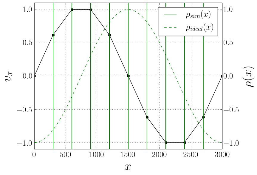
(a) PIC

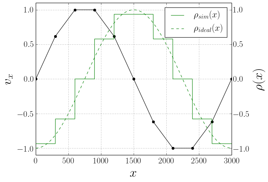
(b) SIC: piecewise constant segments

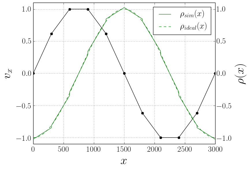
(c) SIC: piecewise linear segments

Figure 1: A comparison of the sheet location in phase space (black connected dots) and the resulting deposited charge density (green) for the old (PIC) method LABEL:sub@fig:old_method_simple, piecewise constant LABEL:sub@fig:piecewise_constant_simple, and piecewise linear segments LABEL:sub@fig:piecewise_linear_simple. Position is measured in units of the cell size $dx$ in this and all other figures. The test case is a cold, sinusoidally perturbed, electrostatic plasma in a periodic region where $n_{ppc}=\frac{10}{3000}\ll 1$. The charge density and velocity are normalized by their maximum value over the simulation region. It is clearly visible how the PIC particles produce very narrow peaks (limited in sharpness by the finite spatial grid). The functional form of the simulated charge density $\rho_{sim}(x)$ only begins to resemble the correct sinusoidal solution $\rho_{ideal}(x)$ once $n_{ppc}$ is set $\gg 1$. By contrast, both SIC schemes achieve a reasonable approximation of the sinusoidal density profile even though there are far fewer particles than cells. The piecewise constant LABEL:sub@fig:piecewise_constant_simple and piecewise linear segments LABEL:sub@fig:piecewise_linear_simple are clearly visible. The piecewise linear scheme visibly captures significantly more information by using gradient information.

2.6 1D Refinement

From the ansatz of assuming a piecewise constant or piecewise linear charge density between two tracers it becomes clear that the accuracy of the method is limited by the spacing of adjacent tracers. If two adjacent tracers move too far apart, then the information about the functional form of the charge density between the two tracers is only zeroth or first order over a wide range, which causes much information to be lost.

For a simulation using the line segment method to accurately evolve the phase space sheet, the length of each individual line segment must thus be comparable to or less than the force resolution of the grid. There are two main cases in which this condition can be violated. The first and simplest case arises when the phase space sheet has a “well-behaved” topology, but there are simply too few tracers. The second case arises when the sheet folds and stretches in phase space in such a way that adjacent tracers move far away from each other. A simulation of plasma instabilities such as the two-stream instability (as discussed in section 3.2) is an example of such complex behavior of the sheet in phase space.

In any situation in which the spacing between connected tracers becomes significantly larger than the grid spacing, it thus might become necessary to implement a refinement scheme in order to accurately continue evolving the system in time. One simple scheme is to have a condition on the maximum segment length (which will depend on the grid spacing). If at any time any segment becomes larger than the maximum length, a new tracer is inserted in the center of the segment (such that the two new segments each carry half of the charge of the old segment). The velocity of the new tracer is initialized to the average of the velocities of the original two tracers. More accurate refinement schemes may also take into account the distance between the tracers in velocity space or the curvature of the phase-space sheet. The simple refinement criterion we have implemented is sufficient for the initial demonstration of the SIC method, and more complex schemes will be investigated in future work.

Figure 2 demonstrates this refinement scheme for five different simulations of the two-stream instability. The simulations all start with 10 particles per cell per stream, but differ in the maximum segment length (referred to as the “refinement length”.) Each simulation was evolved until the refinement factor (current number of tracer particles / initial number of tracer particles) reached $10^{3}$. The refinement factor for each simulation is plotted in figure 2a. During the linear growth phase (which saturates around $t\approx 17.5\,\omega_{p}^{-1}$), the stretching of the line segments is small and there is seen to be little refinement. In the nonlinear regime the streams become severely distorted as a vortex is formed in phase-space. Once this complex structure has begun to develop, the refinement factor grows at an approximately exponential rate. The refinement length controls the time of the onset of exponential growth, but has little effect on the growth rate.

The evolution of the mean line segment length for each simulation, normalized to the refinement length, is plotted in figure 2b. The mean length tends to settle near a value slightly larger than one half of the refinement length for the simulations performed. For the simulation with a refinement length of $1/9$ cells, the mean length initially decreases because its final value is less than the initial particle separation. For the other four simulations the initial particle separation is less than the final mean length, and the mean length is seen to grow from its initial value. The evolution of the length of a representative line segment is shown in figure 2c. This illustrates two important types of events that are characteristic of the evolution of a line segment. During “inversions” the line segment length instantaneously becomes zero, which occurs when the tracer particles that are the endpoints of that line segment cross each other and change their ordering along position space. “Refinements” denote the points in time at which the segment length has grown to be larger than the refinement length, and the line segment is split in two. The evolution plot shown consistently follows the portion of the original line segment associated with a single one of its initial tracer particles.

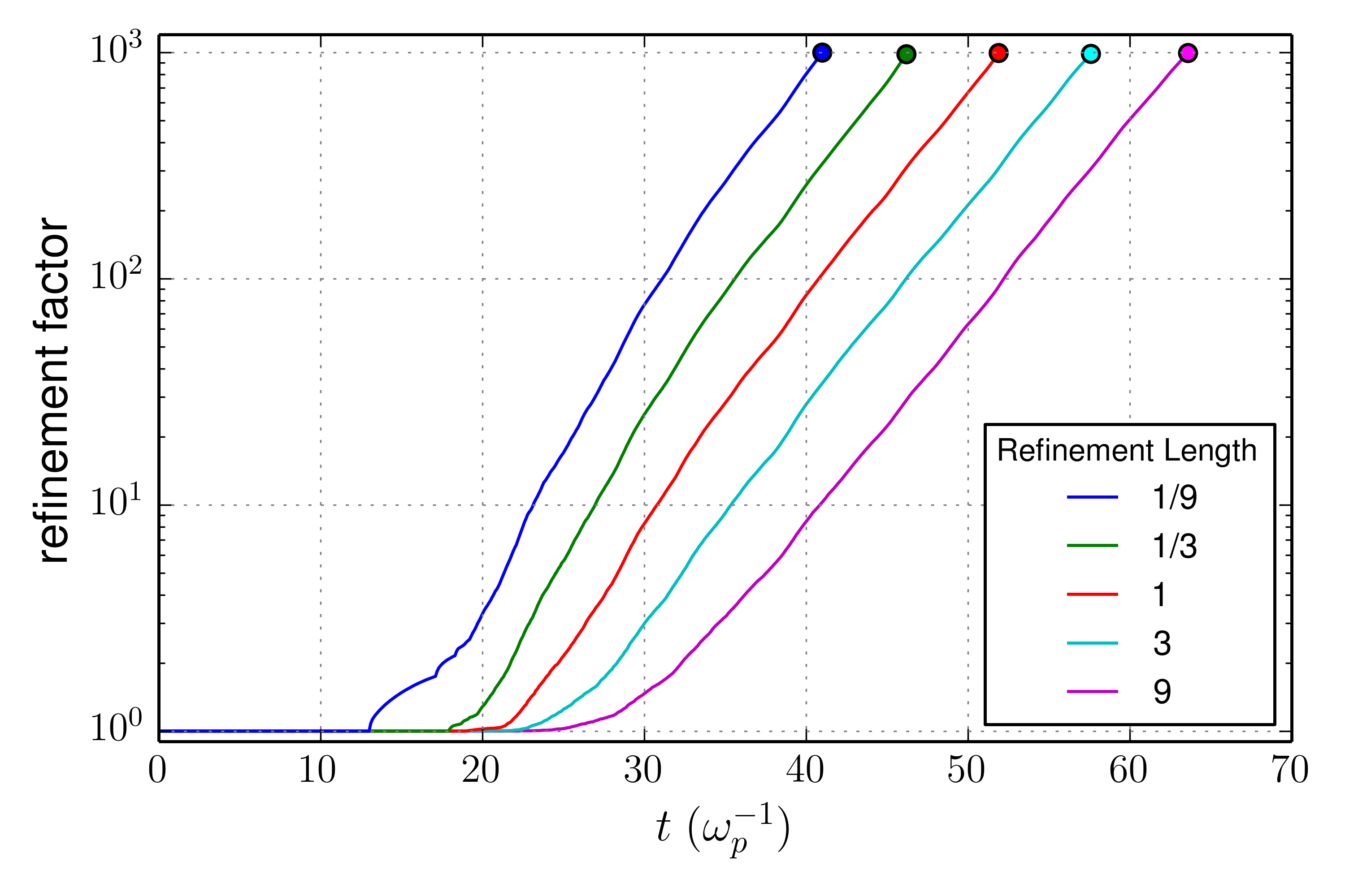
(a)

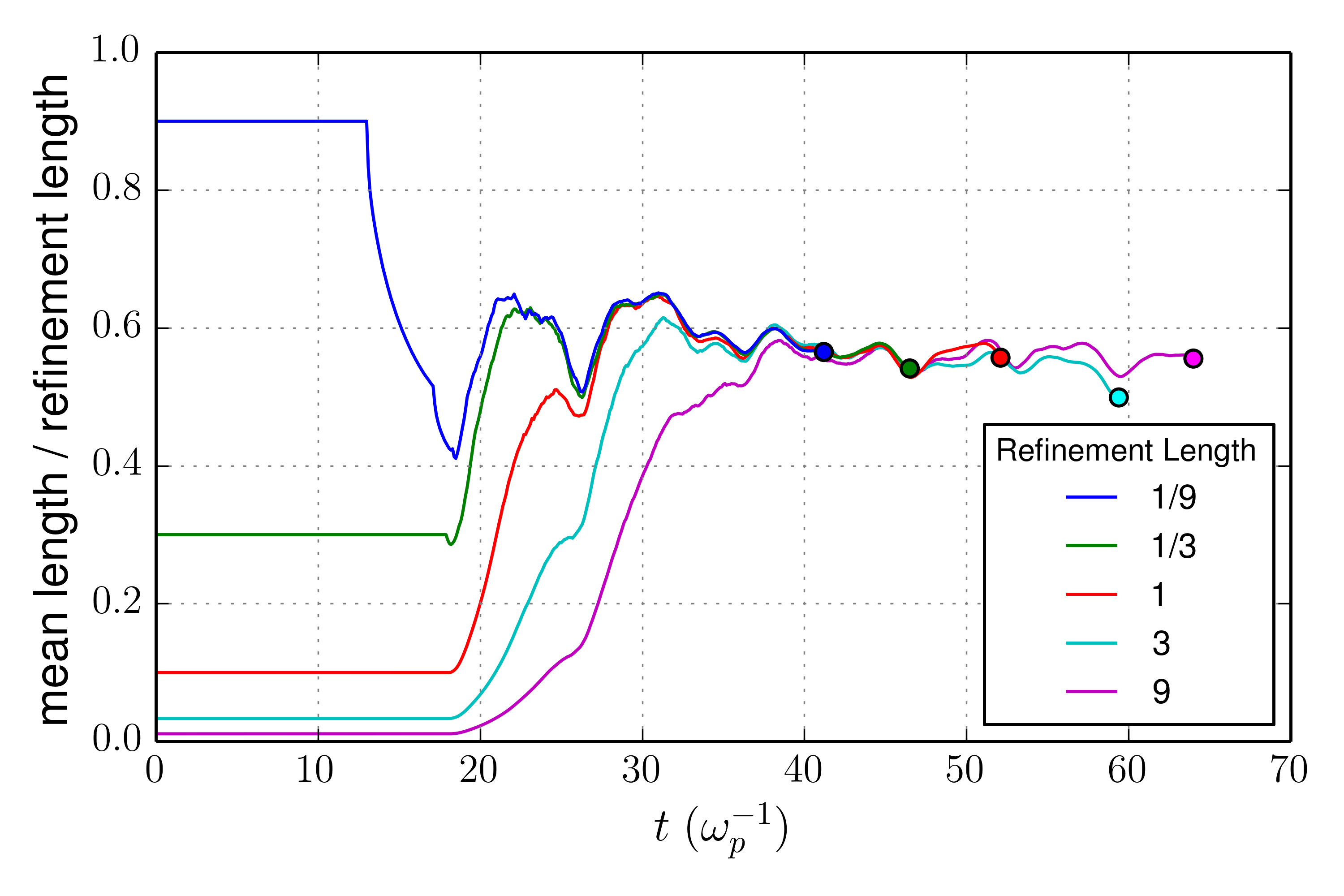
(b)

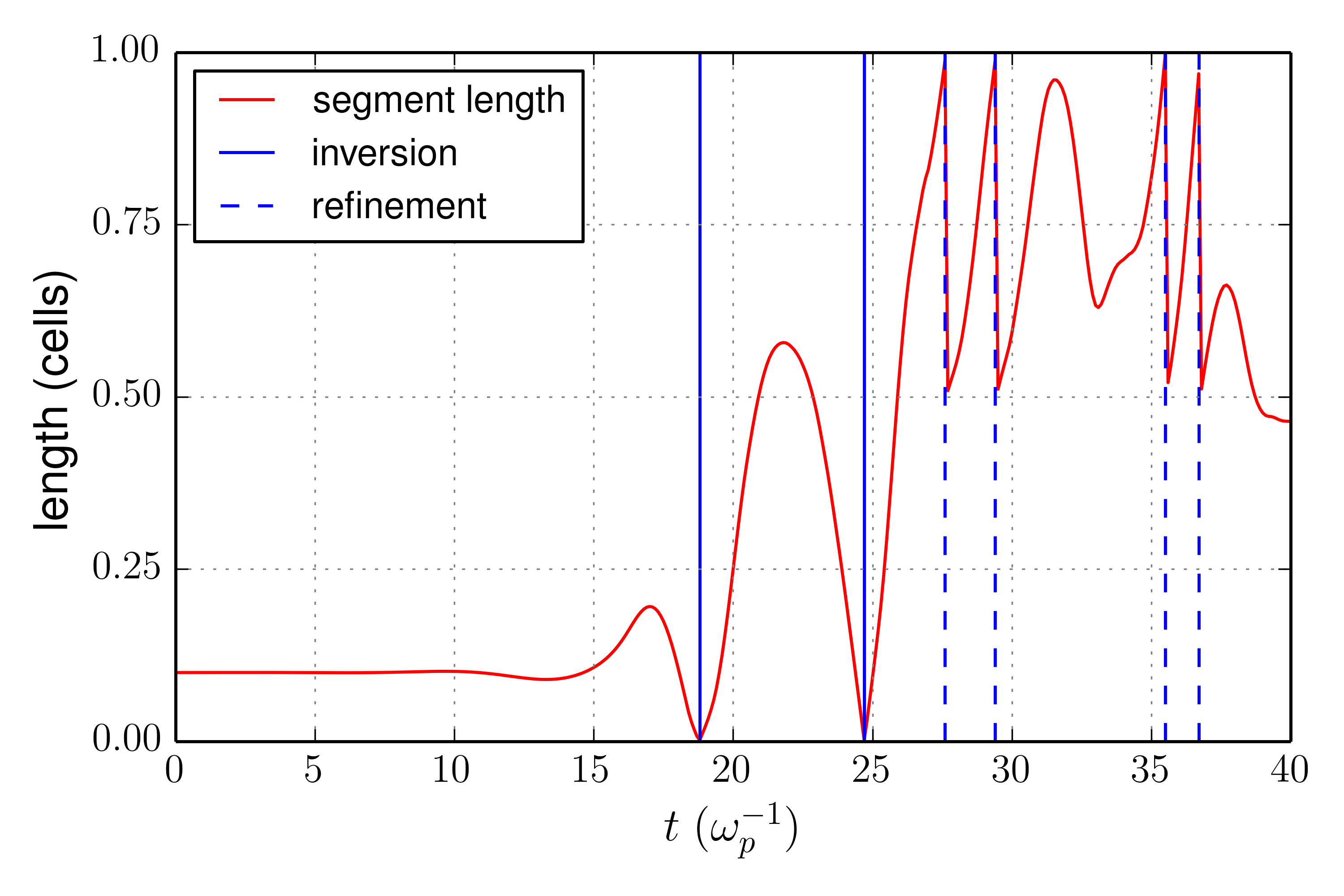
(c)

Figure 2: LABEL:sub@fig:refinement_factor Evolution of the refinement factor (current number of tracer particles / initial number of tracer particles.) In LABEL:sub@fig:refinement_factor and LABEL:sub@fig:mean_length the circles denote the point at which each simulation was stopped. LABEL:sub@fig:mean_length Mean line segment length throughout the simulations, normalized to the refinement length. LABEL:sub@fig:single_segment_length Evolution of a line segment during a simulation with a refinement length of 1 cell length. Inversions mark when the endpoints of the line segments cross each other in position space, and refinements mark when the line segment has grown to be larger than the refinement length and is split in two.

3 1D Neutral Plasma Tests

We now employ a set of standard [54, 55, 56] plasma tests that have been used by several authors to evaluate new codes for the Vlasov-Poisson system. In particular, we use test problems for both warm and cold plasmas. We compare our own implementation of the SIC method with a standard PIC code. Both codes are identical, except for the scatter step (see section 2.3), which is performed according to the scheme in question.

In one dimension, the simplex is a line segment. Thus, the $M$ manifolds with which we discretize the initial phase space density are one dimensional lines moving in the associated two dimensional phase space. For a cold plasma (zero temperature) we can in fact start with the single sheet case ($M=1$) before moving to cases with $M>1$. In fact, let us start with a uniform medium of charge density everywhere and the cold initial phase space distribution

$$f(x,v)=\rho_{0}(x)\delta\left(v-v_{s}-v_{1}\sin(2\pi x/L)\right)$$ (16)

where $L$ is the length of the simulation region.

3.1 Plasma Oscillations of a Cold Sheet

We apply the above described density assignment algorithm to the test case of electron plasma oscillations in a 1D plasma with periodic boundary conditions. We assume that the immobile ions produce a uniform positive charge background. We take $v_{s}=0$ and $v_{1}$ in equation (16) of some small value to study the evolution of plasma waves in our system. This corresponds to a uniform space charge density and a sinusoidal perturbation of magnitude $v_{1}$ to the velocities. In that case, we expect simple standing electrostatic oscillations. In particular, the velocity distribution in phase space, $v(x,t)$, will analytically have the form

$$v(x,t)=v_{1}\sin(2\pi x/L)\cos(\omega_{p}t)\;,$$

where $\omega_{p}$ is the plasma frequency. We can now compare both SIC and PIC to the analytical solution. The results are summarized in figure 3, where we study the error in potential energy. The new scheme performs much better than PIC at lower particle numbers, while both schemes approach the same base-line performance as the particle number becomes very high, confirming consistency. At high particle numbers, the error baseline is due to the grid discretization of the simulation region into cells. This baseline error of course drops as the number of cells is increased.

While this and the following tests focus mainly on the potential energy evolution $E_{pot}(t)$, this is just one of many possible testing grounds for the algorithm that we picked out for clarity and consistency. In this and the following investigations, we also monitored our algorithms for conservation of total momentum and energy. While SIC is neither explicitly momentum conserving (due to the lack of symmetry between the charge scattering and the force gathering steps) nor energy conserving, we find in all tests that both total energy and total momentum are conserved very well and always at least as well as in PIC with the same number of particles.

We also studied the computational cost of PIC and SIC in all of our test problems. While these cases may not be entirely representative of large-scale, state of the art computational plasma physics tasks, we find as expected that PIC and SIC require nearly the same computational time for given values of $n_{ppc}\gtrsim 1$ and $n_{cells}$. PIC runs faster for $n_{ppc}<<1$ (because SIC requires touching all cells, even in this regime, while PIC only touches a small constant number for each particle), but in this regime PIC is highly inaccurate even for the simplest test cases.

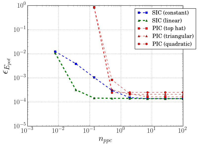
(a) Error Convergence as a function of $n_{ppc}$ ($n_{cells}=389$).

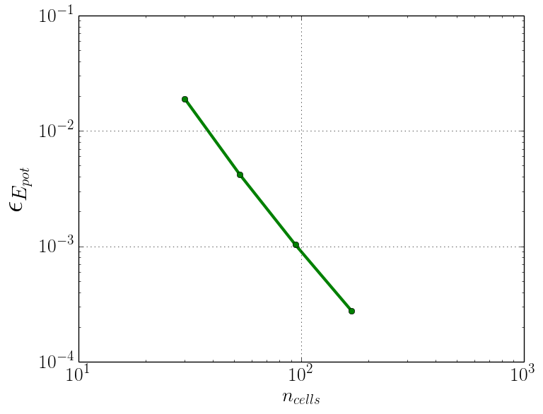
(b) Error Convergence as a function of $n_{cells}$ ($n_{ppc}=100$)

Figure 3: LABEL:sub@fig:e_pot_error_simple The error in the potential energy evolution $\epsilon_{E_{pot}}$ for the old (PIC) and new (SIC) schemes as a function of particle number per cell. We employ CIC (“top hat”), triangular (“triangular”) and “quadratic” (i.e. cubic interpolation) particle shapes for PIC. We compare against SIC with the two cases of piecewise linear and piecewise constant charge densities on the segments. Both PIC and SIC converge to nearly the same “base-line error”, set by when the error due to the finite grid spacing becomes dominant. However, SIC more rapidly reaches this baseline, especially with linear segments, which offer higher order convergence. Higher order particle shapes for PIC offer slightly lower errors than standard CIC (“top hat”) but converge to a higher baseline error due to their larger size. In LABEL:sub@fig:e_pot_error_simple_cells, we show the common baseline error reached by PIC and SIC as a function of the number of cells. The error was measured as the mean $L_{1}$ difference over one plasma period between $\tilde{E}_{\rm{pot}}(t)$ as obtained from the simulation and the analytical solution $E_{\rm{pot}}(t)=\sin^{2}(\frac{2\pi t}{T_{p}})E_{tot}$, where $T_{p}$ is the analytical value for the plasma period.

Figure 4 shows a comparison of phase-space after one plasma oscillation for two simulations, one using PIC with 510 particles per 50 cells and the other using SIC with 51 particles per 50 cells. These choices of parameters result in the initial number of particles per cell not being uniform across the grid. In the PIC simulation, significant noise from grid heating [57] has developed in phase-space after only one plasma oscillation period. This noise is eliminated when the system is evolved using SIC, even with one-tenth the number of particles. We used linear particles (“top hat” shape) for PIC. For higher-order particles the noise is less pronounced, but it still arises if we decrease the number of particles to near $n_{ppc}=1$. SIC remains without noise even in this regime. While SIC (because of its linear interpolation) may theoretically be subject to the grid heating instability just like PIC is, we find in our tests that SIC is much less exposed to this problem.

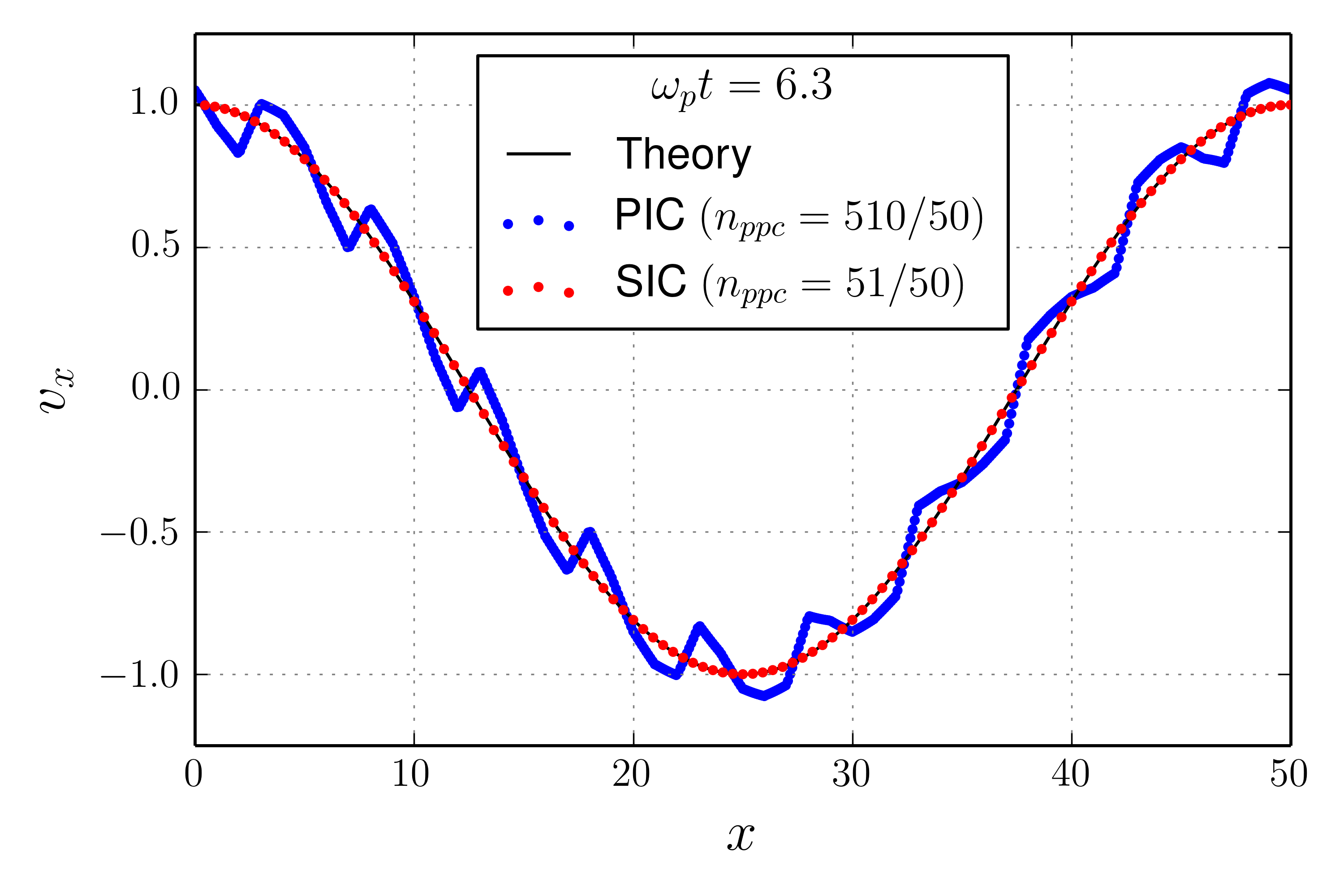
Figure 4: Comparison of phase-space for PIC with linear particles (“top hat” shape) and SIC with constant segments after one plasma oscillation period. The velocity scale is in units of the initial velocity perturbation amplitude $v_{1}$. The grid induced noise seen when using PIC is absent in the simulation performed with SIC, even with $1/10$ the number of particles.

3.2 Two-Stream Instability

As a classic test problem that exhibits nonlinear evolution of the distribution function, we perform simulations of the two-stream instability and compare the SIC and PIC methods to each other and to theory [58] . Linearizing the system of equations describing two cold plasma streams with equal densities and opposite velocities $v_{0}$ in a uniform background of ions gives the following dielectric function:

$$\frac{1}{\epsilon_{0}}\epsilon(\omega,k)=1-\frac{\omega^{2}_{p}}{(\omega+kv_{0})^{2}}-\frac{\omega^{2}_{p}}{(\omega-kv_{0})^{2}}$$

For electrostatic (longitudinal) oscillations, setting $\epsilon(\omega,k)=0$ gives a quartic equation for $\omega$ that leads to four dispersion branches, with unstable modes existing for

$$k<\frac{\sqrt{2}\omega_{p}}{v_{0}}$$

In our simulations the distribution function is initialized as

$$f(x,v)=\delta(v\pm v_{0})(1+\epsilon\cos(kx))$$

where the perturbation wave vector $k$ is chosen to excite the mode with the maximum growth rate. According to the dispersion relation, this mode will have a growth rate of

$$\operatorname{Im}[\omega_{max}]=\frac{\omega_{p}}{2}\;.$$

The size of the simulation box is chosen such that the wave vector in question also corresponds to the fundamental mode of the box.

Figure 5 shows a comparison of the time evolution of the electric field energy for the two methods, for simulations with $0.1$ particles per cell per stream. Both methods are able to accurately capture the exponential growth of the excited component of the electric field, giving a rate that closely agrees with the analytical prediction. However, only the SIC method is able to correctly reproduce the evolution of the total electric field energy. When using the PIC method, such low particle numbers result in a very noisy charge density and resulting electric field, exciting many modes other than just the fundamental that was explicitly excited in the initialization of the distribution function. The presence of these higher modes in the electric field will cause effects on small spatial scales that do not accurately model the intended distribution function, where these modes are not present. Whenever such spatial scales are of interest, the SIC method has the clear advantage that it is able to accurately evolve the distribution function at particle numbers much lower than possible using the PIC method, reducing the computational cost of the simulation. This point is also confirmed figure 6. Only with much higher number of particles is the lower-wavelength noise removed when using PIC.

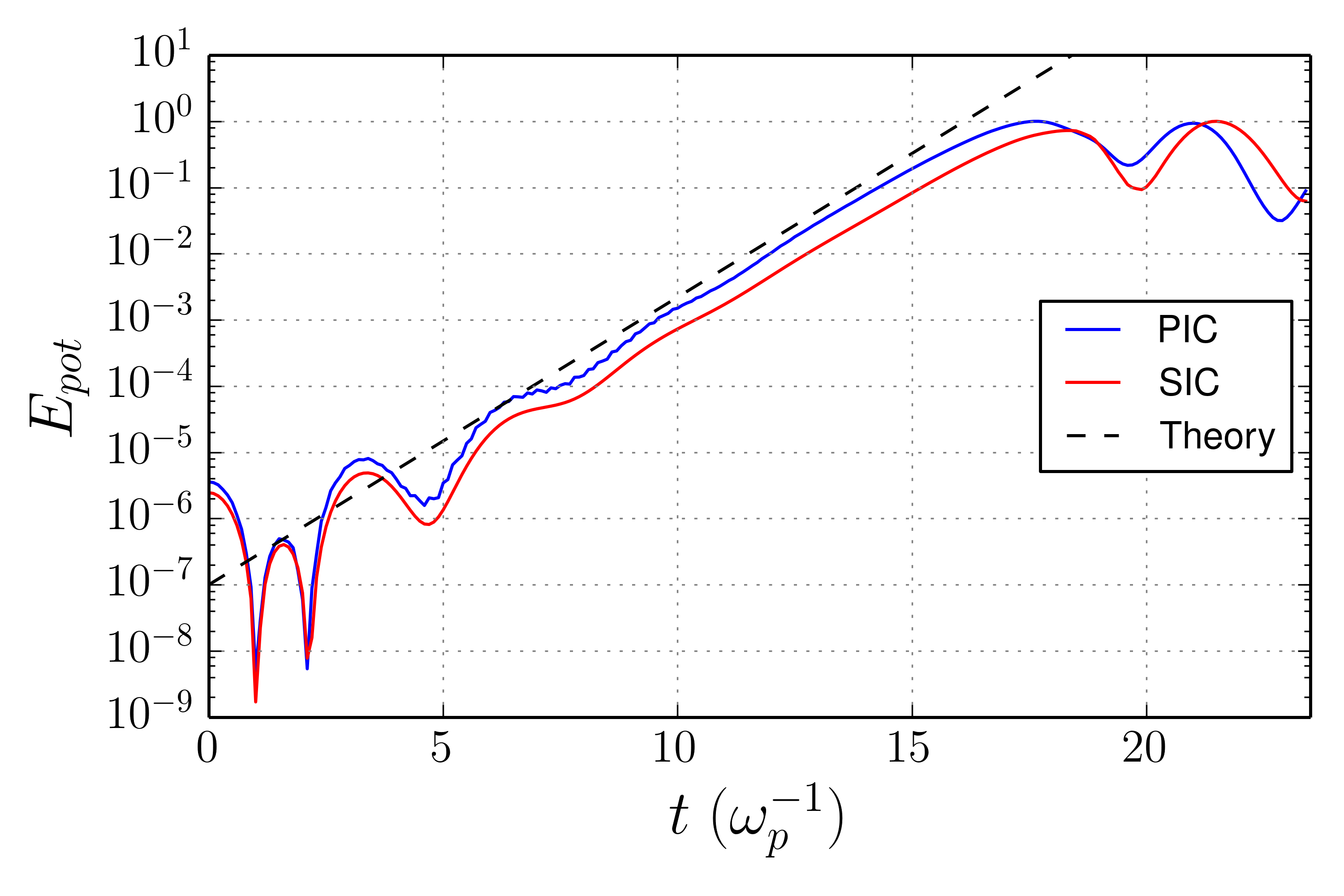
(a) Energy in the excited mode of the electric field

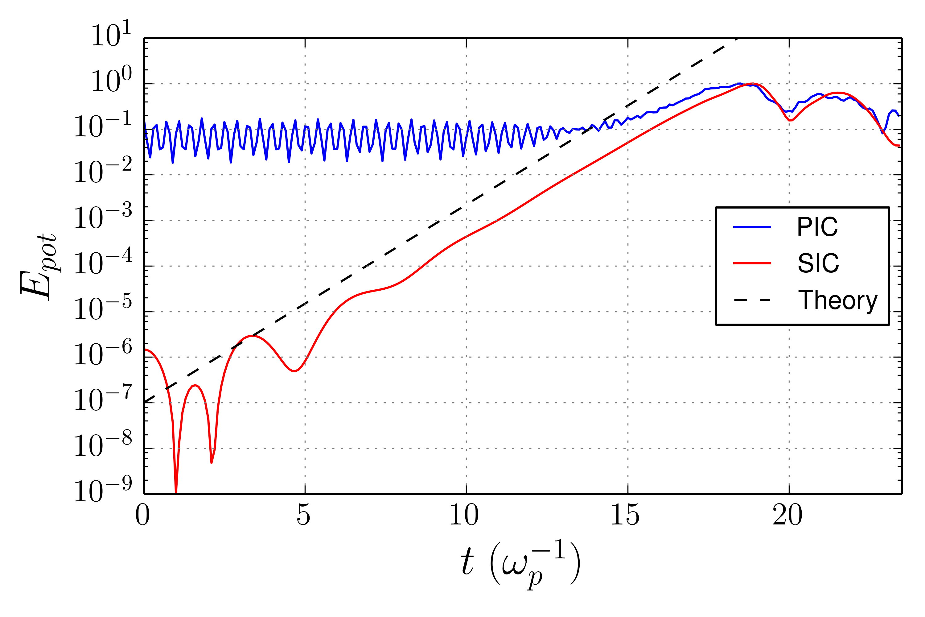
(b) Total electric field energy

Figure 5: Evolution of the energy in the excited component of the electric field and the total energy in the electric field during a two-stream instability. The simulations have $0.1$ particles per cell per stream, for both SIC and PIC. Although both methods accurately reproduce the exponential growth of the excited mode, the noise introduced by PIC excites many other spurious modes, and thus only SIC is able to correctly reproduce the growth of the total electric field energy.

The SIC method is able to accurately simulate the initial linear growth of the instability without refinement of the line segments, (as shown in figure 5 where no refinement was used for the SIC method). However, after the linear growth saturates the line segments begin to rapidly expand as a vortex develops in phases space that continuously stretches the phase space sheets of the two streams. Once a single line segment has expanded to the size of the simulation box, the simulation can no longer continue as it is not possible to contain a line segment larger than the periodic simulation region. This problem is overcome by refining the line segments based on a refinement length criteria, allowing the simulation to proceed into the nonlinear regime. As shown in figure 2, when using refinement to simulate into the nonlinear regime, the number of line segments grows approximately exponentially with time. The length of time that the simulation is able to proceed is then limited only by the available computational resources. While the exponential growth in the number of particles means that the SIC method will be more expensive computationally than the PIC method when applied to the two-stream instability, the SIC method retains the intricate phase space structure that develops as the vortex wraps and folds the phase space sheets of the two streams into each other. This information is completely lost when using the PIC method, likely reducing the accuracy of simulations in the nonlinear regime.

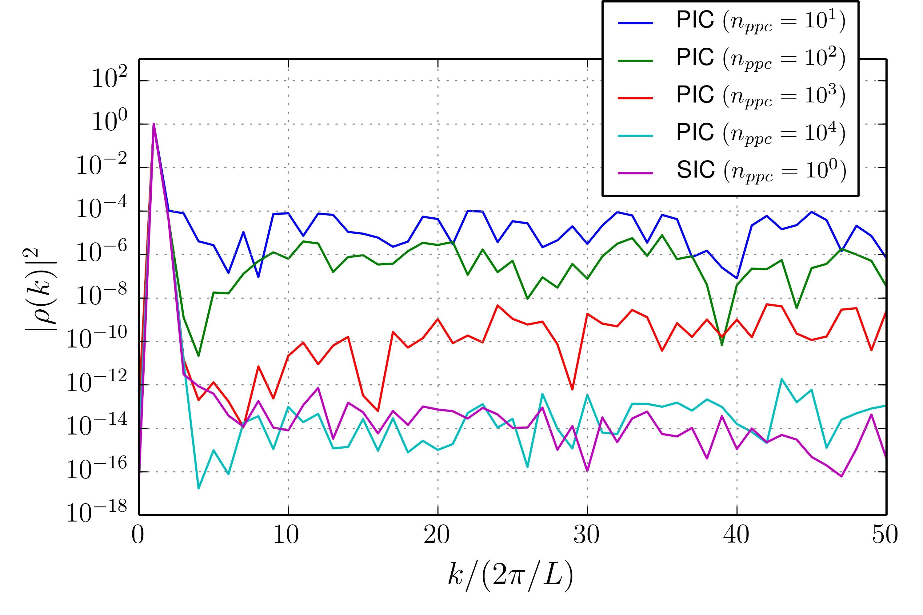
Figure 6: Fourier transform of the charge density in the simulation of the two-stream instability. The charge density is a snapshot in time during the linear growth phase of the instability. Note that in addition to the explicitly excited mode, there is significant noise in many other higher modes for PIC. Only with high particle numbers does the noise level approach that of SIC.

3.3 Landau Damping

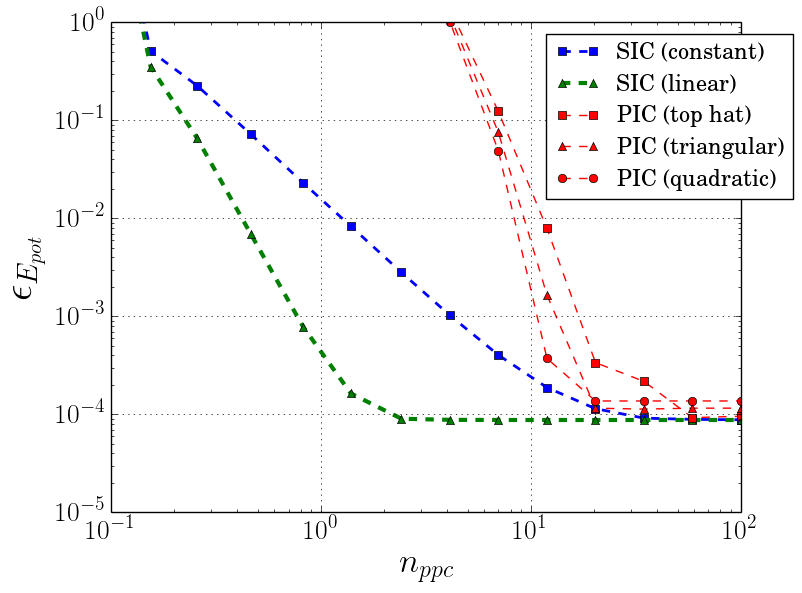
(a) Error Convergence as a function of $n_{ppc}$ ($n_{cells}=389$)

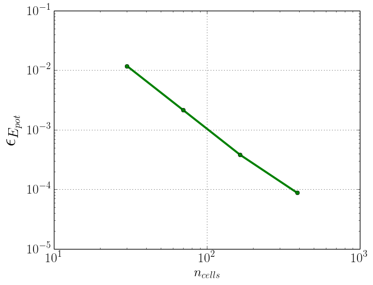
(b) Error Convergence as a function of $n_{cells}$ ($n_{ppc}=100$)

Figure 7: LABEL:sub@fig:e_pot_error_landau Error convergence comparing the SIC method to the standard PIC method in the Landau damping problem. The figure has the same style as figure 3. Note how the new scheme converges faster, requiring far fewer particles than the old scheme for equivalent errors. Note also the increase in convergence order when moving from piecewise constant to piecewise linear segments. A minimum error is reached by all schemes as in figure 3 due to the discretization of the simulation region into cells. As the number of cells is increased, this “baseline error” decreases. The baseline error is plotted in LABEL:sub@fig:baseline_error_landau as a function of the number of cells. As the number of cells is increased further, the error again reaches a minimum (around $n_{cells}\sim 750$) due to the finite number of streams and the finite timestep. The convergence was obtained by comparing the evolution of $E_{\rm{pot}}(t)$ during the simulation to a “gold” run with very high particle number. The error represents the mean $L_{1}$ difference between $E_{\rm{pot}}(t)$ during a given run and $E_{\rm{pot}}(t)$ for the gold run. In this case, the gold run was performed with the old (PIC) scheme. $M=20$ streams were used. These results show that in this problem SIC can outperform PIC in accuracy with far fewer resources.

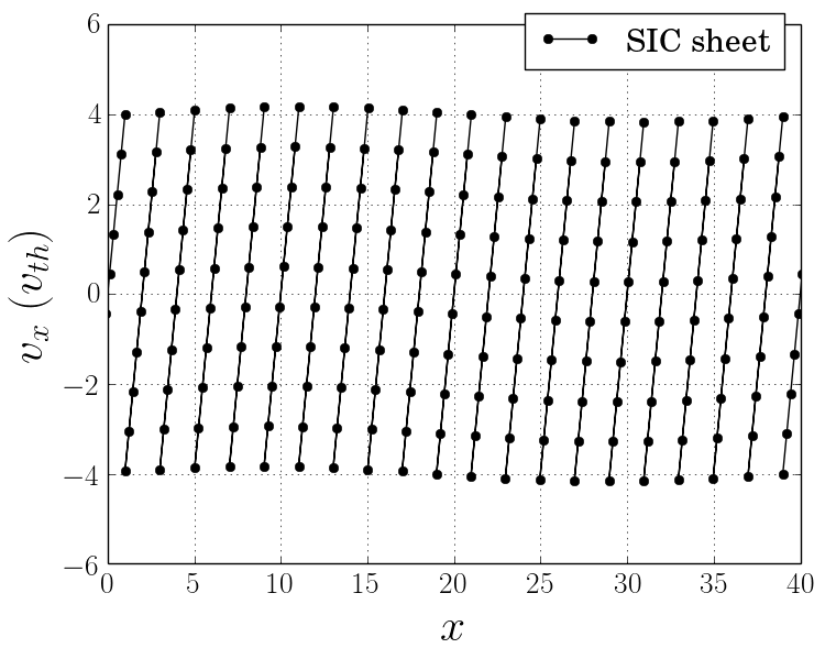
(b) vertical streams

Figure 8: A comparison of the geometry and connectivity of the SIC sheets in phase space for the case of “horizontal” and “vertical” streams. Velocity is measured in units of the thermal velocity. The phase space geometry represents a sinusoidally perturbed warm plasma with $M=10$ streams and $n_{ppc}=200$ particles per cell (distributed over the streams). The positions of the tracers in phase space are identical in both cases, but the connectivities are different: in the horizontal case, we have $10$ sheets with $20$ particles in each of them. In the vertical case, we have essentially $20$ vertical sheets, with $10$ particles in each of them. Both are shown one timestep after the beginning of the simulation. With periodic boundaries the connectivity of course “wraps around” the simulation region. As the simulation progresses, the horizontal streams advect and retain their shape approximately, while the vertical streams tilt to the right and stretch linearly in time.

While we have discussed only cold plasma distributions so far, our method allows modeling of warm plasmas as well and we have have multiple ways of describing such warm plasmas. We will use the example problem of a Landau-damped electrostatic wave in a warm plasma to study the behavior of our method. In particular, we will discuss two extreme cases of setting up the sheet connectivity for modeling the Maxwellian velocity distribution. First, we will consider the perhaps more natural case with $M$ “horizontal” sheets of respectively constant but differing velocities set up parallel to the position axis. These sheets are evenly spaced in velocity space and the tracers within the sheets are evenly spaced in position space. We decrease the mass (and charge) of the particles in sheets with higher velocity to model the Maxwellian density in velocity space. In the second case, we consider $M$ “vertical sheets” starting out parallel to the velocity axis connecting particles with initially equal positions in position space across velocity space. Within the sheets, the particles’ mass (and charge) decreases with velocity to model the Maxwellian distribution. We then perturb the warm distribution with a global velocity mode in order to study Landau damping in this situation. Figure 8 shows the phase space geometry and connectivity of the two approaches.

We use the “cold start” technique of loading $M$ cold sheets of particles in the PIC comparison as well. This is a standard approach [59] and stands in contrast to the “warm start”, where the particles are distributed more randomly in velocity space. The trade-off is between an additional randomization of the particles, which fills in the gaps in velocity space better but incurs additional numerical noise — which might overwhelm the electrostatic perturbation to be studied — on the one hand, and the progression of the multi-beam instability on the other hand. For all methods, we expect our solutions to converge to the continuum solution as an increasing number of streams in velocity space are used [20].

3.3.1 Convergence Study

In order to quantify the error of our simulation, we perform one “gold run” and measure the potential energy as a function of time $E_{\rm{pot}}(t)$ over one plasma period. This gold run has high values for all relevant parameters determining accuracy, i.e. the number of particles per cell $n_{ppc}$ and the number of simulation cells $n_{cells}$. We then compare other solutions for $E_{\rm{pot}}(t)$ from other runs to this gold run by integrating the $L_{1}$ error over $t$. This allows us to study the error convergence rate. The gold run is performed with the standard PIC scheme. We perform this error convergence study for both piecewise constant segments and piecewise linear segments, as discussed in sections 2.3 and 2.5, respectively. The results are summarized in figure 7.

As expected, the error decreases with increasing particle number for both schemes, until it converges to a minimum error produced by other factors, such as the the finite number of grid points. The figures show that the new scheme requires far less particles to converge to the minimum error than the old scheme does. The plot further suggests that for SIC at low particle numbers, where the error due to the particle spacing is dominant, the error drops with a fixed power law, i.e. a fixed linear slope on the logarithmic plot. Denoting the total number of particles per cell as $n_{ppc}$ and the error in the potential energy as $\epsilon_{E_{\rm{pot}}}$, we postulate

$$\epsilon_{E_{\rm{pot}}}\propto n_{ppc}^{\gamma}\;,$$

where $\gamma$ denotes the rate of convergence of the method.

Note that the convergence rates as can be read off from the slopes of the error functions are consistent with first order convergence ($\gamma=-1$) for the piecewise constant segments and second order convergence ($\gamma=-2$) for the piecewise linear segments. The actual slope in the potential energy error plot is twice this value. To explain this, take $\tilde{E}_{\rm{pot}}(t)$ to denote our estimate in the simulation for the potential energy as a function of time. Moreover, let $\tilde{E}(x,t)$ denote our simulation estimate of the electric field, which we write as the true electric field $E(x,t)$ plus an error term $\epsilon(x,t)$. We then find that the first order error term integrates to zero and we are left with a term of twice that order:

$$\tilde{E}_{\rm{pot}}(t) = \int_{0}^{L}\tilde{U}(x,t)dx\propto\int_{0}^{L}(\tilde{E}(x,t))^{2}dx$$

$$= \int_{0}^{L}(E(x,t)+h^{d}\epsilon(x,t))^{2}dx$$

$$= E_{\rm{pot}}(t)+h^{d}\int_{0}^{L}E(x,t)\epsilon(x,t)dx+h^{2d}\int_{0}^{L}\epsilon(x,t)^{2}dx$$

$$= E_{\rm{pot}}(t)+h^{d}\langle E(x,t)\epsilon(x,t)\rangle_{x}+h^{2d}\epsilon_{E}(t)$$

$$\approx E_{\rm{pot}}(t)+h^{2d}\epsilon_{E}(t)$$

In the first line, we take $\tilde{U}(x,t)$ as the potential energy density. In the second line, we keep only the lowest order error term, which we assume to be proportional to some step size $h$ at order $d$. In the second to last line, we denote $\langle...\rangle_{x}$ as the average over $x$. Since the electric field and the error in the electric field are uncorrelated, this term approaches zero. This shows that it was OK to include only the lowest order term in the second line — the linear term involving any higher order error would have integrated to zero as well and left a term of twice that order.

We also computed the error in the charge density as a function of the number of particles per cell, and the results are consistent with those for the potential energy.

Several results are important to point out. Once the number of particles is large enough, the error is dominated by the finite grid spacing. As we increase the number of grid cells, this error baseline drops. It drops by the same amount for both schemes, showing that the primary source of improvement in the SIC scheme comes from reducing the “shot noise” associated with too few PIC particles. The smaller amount of particles required for accurate SIC simulations is an especially useful feature, since the number of particles is usually the major limiting computational factor for large-scale simulations. The errors produced by the grid spacing are consistent with second order convergence in $n_{cells}$, for both PIC and SIC.

For piecewise constant segments in figure 7, the error is lower than in the PIC simulation for the same number of particles per cell. Equivalently, far fewer particles than with PIC are required for the same error. For the piecewise linear segments, the effect is even more pronounced: the convergence rate is increased, and even fewer particles are required for the same error. Moreover, the minimum error for a given cell number is reached sooner. Since the total number of particles per cell is measured by $n_{ppc}$, and these particles are distributed over all $M=20$ streams, figure 7 shows that around one particle per cell in a given stream is sufficient for error convergence.

Finally, our data also shows that the error reaches a baseline (for $n_{cells}\approx 750$) at which it is limited by neither $n_{cells}$ nor $n_{ppc}$. We find that the error is now in fact dominated by the number of streams $M$, i.e. the coarse discretization of the distribution function in velocity space.

(a) horizontal streams

(a) Nonlinear Damping

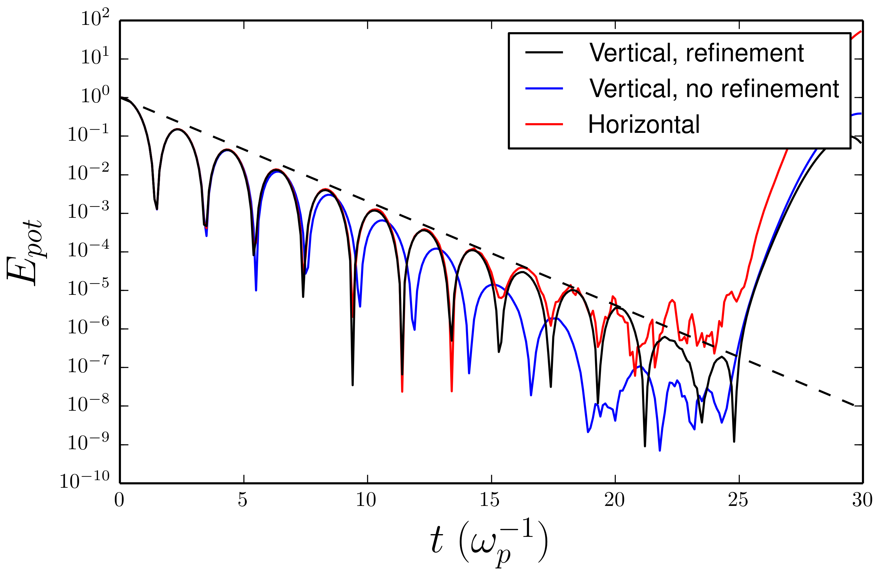
(b) Linear Damping

Figure 9: We illustrate the tradeoff among different setups of the phase space geometry with the example of Landau damping with $M=26$ streams and $160$ particles in every stream. We use the horizontal and vertical setups as shown in figure 8: the tracer particles have the same initial positions in both cases, but the connectivities are different (i.e. for the vertical space, we end up with $160$ vertical streams, with $26$ particles each). The horizontal streams tend to show noise once the multistream instabilities between the different streams develop. The vertical streams are not as affected by this. However, as the vertical streams stretch in phase space, the particle spacing becomes large and information is lost. Once the particle spacing becomes too large, noise develops as well. LABEL:sub@fig:nonlinear_regime A large velocity perturbation gives rise to nonlinear landau damping. We add an exponential trendline to guide the eye. In this regime, the multistream instability develops rapidly and the horizontal streams become noisy. The vertical streams are not subject to this noise. LABEL:sub@fig:linear_regime A small velocity perturbation gives rise to linear landau damping. The horizontal streams remain without noise for a long time, while the vertical streams begin to show inaccuracies earlier (this is set by the time at which the initial particle spacing becomes comparable to the size of the box. However, as we add refinement, this problem is mitigated, and the vertical streams perform very well. For horizontal streams, the lack of refinement is never an issue, as the multistream instabilities would develop anyways. We also studied the above two cases using refined horizontal streams, and as expected the results were nearly identical to the unrefined case. This simple test problems illustrates that the phase space connectivity of the sheets is an algorithmic choice and can depend upon the problem in question.

3.3.2 Phase Space Geometry

We performed an additional investigation to illustrate the flexibility and universality of dealing with connected sheets in phase space. So far, we had connected sheets along lines of constant velocity, so that the tracer spacing would stay small and constant for as long as possible. . However, this is not a requirement. To illustrate this, we perform the same simulation of Landau damping as before, however, this time we compare horizontally connected sheets with (initially) vertically connected sheets. A representation of the potential energy over time the runs is given in figure 9. For horizontally connected sheets, the multistream instability [20] develops between the streams which produces noise in the solution. This instability is not as prominent when the sheets are vertically connected (they simply become broader and flatter lines). On the other hand, vertically connected sheets produce noise when they become too stretched in phase space and the particle spacing becomes comparable to the box size (most information is lost in this case). This problem can be avoided with refinement. Figure 9 shows that different test problems cause one method to perform better than the other.

This toy example illustrates a key point. The connectivity in phase space of the sheets is an algorithmic choice. All simulations should in the limit approach the same solution. However, given finite computational resources, while it does not reflect any physical discretization, it is a choice that can affect the quality of the solution. There are many sensible ways of picking the connectivity, and in general the optimal connectivity will depend on the specific application.

4 Discussion and Conclusions

The SIC method represents an alternative discretization of phase space that offers merits over the traditional PIC method. In particular, for problems in which there is no turbulence or folding of sheets in phase space, SIC offers higher accuracy than PIC with significantly fewer tracer particles. Using first order information, SIC only requires the particle spacing to be sufficiently small to allow a reasonable piecewise linear approximation of the phase space density. Thus, a single particle for a few simulation regions is usually sufficient and at most one particle per simulation region is beneficial for error reduction, because the discretized simulation space cannot resolve lower-wavelength features either way. By contrast, PIC requires many tens of particles per simulation region. Since the simulation region spacing must itself be chosen to resolve the smallest scale of interest in the phase space distribution, this requirement results in orders of magnitude higher particle numbers. We have demonstrated this in several test problems, both for thermal and cold phase space distributions. Moreover, the computational effort per particle is nearly identical to PIC. Since particles are the main resource limitation for most large-scale simulations, a reduction in the required amount of particles is encouraging for the community.

Since the algorithms for PIC and SIC differ only in the charge deposit, it is worthwhile to consider a bit more closely the performance differences in this step. The cost for PIC is directly proportional to the number of particles, since each is deposited into a small and constant number of cells. For SIC, for $n_{ppc}<1$ we can have one particle “touching” many cells, while a single particle will only touch a small number of cells if $n_{ppc}\gtrsim 1$ (since the average particle spacing is less than one cell). Thus, for $n_{ppc}>1$ the cost is proportional to the number of particles as in PIC, while for $n_{ppc}<1$, we have essentially a baseline cost equivalent to $n_{ppc}=1$, because every cell needs to be touched, even when we have few particles. Despite this baseline cost, SIC can offer large savings over PIC for a given problem: as we have demonstrated — for a fixed, small error tolerance — SIC can be run effectively in the regime where $n_{ppc}\sim 1$, whereas PIC requires $n_{ppc}\gg 1$. Because in these regimes both have a computational cost $\sim n_{ppc}$ with a similar cost per particle, SIC offers significant savings. This is true in one dimension and increasingly so in higher dimensions. For nonlinear problems in which refinement for SIC becomes necessary, the cost of course increases over time compared to PIC. On the other hand, unlike PIC, SIC is able to resolve fine features in velocity space as long as this refinement is continued.

The key difference between SIC and PIC is that the functional approximation is not a sum of shape functions, but a set of tracers with an associated interpolation that approximates the functional form. When folding and turbulent motion occur in phase space, the spacing between particles in the phase space sheets becomes unfavorable for an accurate deposit. In particular, as tracers move very far apart from each other, information about the distribution function between the tracers is lost. This can be corrected for with a refinement scheme. It is reasonable to make the refinement criterion based on the distance between tracers. We demonstrate the efficacy of refinement in problems with significant phase space folding and stretching. While refinement increases the computational cost of SIC simulations, the method in turn is able to capture the increasing complexity of the phase space distribution function over time as long as refinement is applied. This stands in contrast to other methods like PIC where this information is lost.

While our general method seems natural and intuitive in one dimension, it is also efficiently extensible to higher dimensions. In general, in $n$ spatial dimensions we are tracking connected phase space sheets that divide position space into $n$-simplices (for example, in $3$ spatial dimensions, we would have a division of position space into tetrahedra).

The phase space sheets in our method are functionally similar to the phase space contours in the so-called “waterbag” method [60]. However, in $n$ spatial dimensions, the phase space sheets only define several manifolds of connected $n$-dimensional simplices, whereas the waterbag method requires manifolds of $2n$-dimensional polyhedra. Thus, our method — with its reduced curse of dimensionality — is easier extended to higher dimensions.

Encouragingly, it is possible to efficiently find the exact intersection of arbitrary polyhedra with cubic meshes [61]. This of course enables the exact SIC charge deposit step in higher dimensions. It is also possible to deposit higher dimensional polyhedra with linear fields onto cubic meshes [62]. The gradient for the linear fields can be found either by fitting an $n+1$ dimensional hyperplane to neighboring points, or by a generalization of finite differences [63]. It is thus viable and realistic to efficiently extend SIC (including piecewise linear segments) to higher dimensions. It is reasonable to assume that the sparsity of the representation of the distribution function will be even more beneficial for resource savings in these higher-dimensional spaces.

In general, SIC can be interpreted as removing some redundant information in the PIC description of phase space densities. The $2n$ dimensional functional form of the distribution function is approximated using a set of smooth $n$ dimensional manifolds. These smooth manifolds in return are approximated using a sufficient but not redundant number of tracer particles. This stands in contrast to PIC where the entire distribution function is Monte-Carlo sampled. From this perspective it is clear why the removal of redundant information results in higher efficiency encoding of the information contained in the phase space distribution function. However, as the true evolution of the distribution function surpasses the complexity that can be adequately captured by the set of available manifolds and their respective tracer particles, refinement is necessary in order to retain accuracy. Unrefined SIC should be viewed as an attempt of more efficiently encoding high-dimensional information.

While it of course does not represent a universal reduction in the complexity of representing the Vlasov-Poisson system numerically, SIC offers merits in terms of both physical accuracy and computational cost across a range of practical problems.

References

- [1] T. Abel, O. Hahn, R. Kaehler, Tracing the dark matter sheet in phase space, MNRAS427 (2012) 61–76. arXiv:1111.3944, doi:10.1111/j.1365-2966.2012.21754.x.
- [2] O. Hahn, T. Abel, R. Kaehler, A new approach to simulating collisionless dark matter fluids, ArXiv e-printsarXiv:1210.6652.
-
[3]
F. Chen, Introduction to
Plasma Physics and Controlled Fusion, no. v. 1 in Introduction to Plasma
Physics and Controlled Fusion, Springer, 1984.
URL http://books.google.com/books?id=ToAtqnznr80C -
[4]
B. Cerutti, G. R. Werner, D. A. Uzdensky, M. C. Begelman,
Gamma-ray
flares in the crab nebula: A case of relativistic reconnection, Physics of
Plasmas (1994-present) 21 (5) (2014) –.
doi:http://dx.doi.org/10.1063/1.4872024.
URL http://scitation.aip.org/content/aip/journal/pop/21/5/10.1063/1.4872024 -
[5]
L. Sironi, A. Spitkovsky,
Relativistic
reconnection: An efficient source of non-thermal particles, The
Astrophysical Journal Letters 783 (1) (2014) L21.
URL http://stacks.iop.org/2041-8205/783/i=1/a=L21 -
[6]
M. J. Pueschel, D. Told, P. W. Terry, F. Jenko, E. G. Zweibel, V. Zhdankin,
H. Lesch, Magnetic
reconnection turbulence in strong guide fields: Basic properties and
application to coronal heating, The Astrophysical Journal Supplement Series
213 (2) (2014) 30.
URL http://stacks.iop.org/0067-0049/213/i=2/a=30 -
[7]
F. Valentini, A. Vecchio, S. Donato, V. Carbone, C. Briand, J. Bougeret,
P. Veltri, The nonlinear
and nonlocal link between macroscopic alfvénic and microscopic electrostatic
scales in the solar wind, The Astrophysical Journal Letters 788 (1) (2014)
L16.
URL http://stacks.iop.org/2041-8205/788/i=1/a=L16 - [8] E. Esarey, C. Schroeder, W. Leemans, Physics of laser-driven plasma-based electron accelerators, Reviews of Modern Physics 81 (3) (2009) 1229.
-
[9]
F. Fiuza, A. Stockem, E. Boella, R. A. Fonseca, L. O. Silva, D. Haberberger,
S. Tochitsky, W. B. Mori, C. Joshi,
Ion
acceleration from laser-driven electrostatic shocks, Physics of Plasmas
(1994-present) 20 (5) (2013) –.
doi:http://dx.doi.org/10.1063/1.4801526.
URL http://scitation.aip.org/content/aip/journal/pop/20/5/10.1063/1.4801526 -
[10]
A. Kemp, F. Fiuza, A. Debayle, T. Johzaki, W. Mori, P. Patel, Y. Sentoku,
L. Silva,
Laser–plasma
interactions for fast ignition, Nuclear Fusion 54 (5) (2014) 054002.
URL http://stacks.iop.org/0029-5515/54/i=5/a=054002 -
[11]
J. Dawson,
One‐dimensional
plasma model, Physics of Fluids (1958-1988) 5 (4) (1962) 445–459.
doi:http://dx.doi.org/10.1063/1.1706638.
URL http://scitation.aip.org/content/aip/journal/pof1/5/4/10.1063/1.1706638 -
[12]
J. Denavit, W. L. Kruer,
Comparison
of numerical solutions of the vlasov equation with particle simulations of
collisionless plasmas, Physics of Fluids (1958-1988) 14 (8) (1971)
1782–1791.
doi:http://dx.doi.org/10.1063/1.1693676.
URL http://scitation.aip.org/content/aip/journal/pof1/14/8/10.1063/1.1693676 - [13] C. K. Birdsall, A. B. Langdon, Plasma physics via computer simulation, CRC Press, 2004.
- [14] R. W. Hockney, J. W. Eastwood, Computer simulation using particles, CRC Press, 1988.
- [15] J. M. Dawson, Particle simulation of plasmas, Reviews of Modern Physics 55 (1983) 403–447. doi:10.1103/RevModPhys.55.403.
- [16] H. Okuda, C. K. Birdsall, Collisions in a Plasma of Finite-Size Particles, Physics of Fluids 13 (1970) 2123–2134. doi:10.1063/1.1693210.
- [17] A. B. Langdon, C. K. Birdsall, Theory of Plasma Simulation Using Finite-Size Particles, Physics of Fluids 13 (1970) 2115–2122. doi:10.1063/1.1693209.
- [18] J. M. Hammersley, D. C. Handscomb, G. Weiss, Monte Carlo Methods, Physics Today 18 (1965) 55. doi:10.1063/1.3047186.
- [19] J. A. Byers, M. Grewal, Perpendicularly Propagating Plasma Cyclotron Instabilities Simulated with a One-Dimensional Computer Model, Physics of Fluids 13 (1970) 1819–1830. doi:10.1063/1.1693160.
- [20] J. M. Dawson, Plasma oscillations of a large number of electron beams, Physical Review 118 (2) (1960) 381.
-
[21]
G. Knorr,
Plasma
simulation with few particles, Journal of Computational Physics 13 (2)
(1973) 165 – 180.
doi:http://dx.doi.org/10.1016/0021-9991(73)90021-1.
URL http://www.sciencedirect.com/science/article/pii/0021999173900211 -
[22]
J. Whitson, J. Smith, J. Whealton,
Calculations
involving ion beam source, Journal of Computational Physics 28 (3) (1978)
408 – 415.
doi:http://dx.doi.org/10.1016/0021-9991(78)90061-X.
URL http://www.sciencedirect.com/science/article/pii/002199917890061X -
[23]
S. Zaki, L. Gardner, T. Boyd,
A
finite element code for the simulation of one-dimensional vlasov plasmas. i.
theory, Journal of Computational Physics 79 (1) (1988) 184 – 199.
doi:http://dx.doi.org/10.1016/0021-9991(88)90010-1.
URL http://www.sciencedirect.com/science/article/pii/0021999188900101 - [24] N. J. Sircombe, T. D. Arber, VALIS: A split-conservative scheme for the relativistic 2D Vlasov-Maxwell system, Journal of Computational Physics 228 (2009) 4773–4788. doi:10.1016/j.jcp.2009.03.029.
- [25] C. Z. Cheng, G. Knorr, The integration of the Vlasov equation in configuration space, Journal of Computational Physics 22 (1976) 330–351. doi:10.1016/0021-9991(76)90053-X.
-
[26]
N. Besse, E. Sonnendrücker,
Semi-lagrangian
schemes for the vlasov equation on an unstructured mesh of phase space, J.
Comput. Phys. 191 (2) (2003) 341–376.
doi:10.1016/S0021-9991(03)00318-8.
URL http://dx.doi.org/10.1016/S0021-9991(03)00318-8 -
[27]
N. Besse, G. Latu, A. Ghizzo, E. Sonnendrücker, P. Bertrand,
A
wavelet-mra-based adaptive semi-lagrangian method for the relativistic
vlasov–maxwell system, Journal of Computational Physics 227 (16) (2008)
7889 – 7916.
doi:http://dx.doi.org/10.1016/j.jcp.2008.04.031.
URL http://www.sciencedirect.com/science/article/pii/S0021999108002672 -
[28]
F. Engelmann, M. Feix, E. Minardi, J. Oxenius,
Nonlinear
effects from vlasov’s equation, Physics of Fluids (1958-1988) 6 (2) (1963)
266–275.
doi:http://dx.doi.org/10.1063/1.1706724.
URL http://scitation.aip.org/content/aip/journal/pof1/6/2/10.1063/1.1706724 -
[29]
J. W. Schumer, J. P. Holloway,
Vlasov
simulations using velocity-scaled hermite representations, Journal of
Computational Physics 144 (2) (1998) 626 – 661.
doi:http://dx.doi.org/10.1006/jcph.1998.5925.
URL http://www.sciencedirect.com/science/article/pii/S0021999198959253 - [30] E. Camporeale, G. L. Delzanno, B. K. Bergen, J. D. Moulton, On the velocity space discretization for the Vlasov-Poisson system: comparison between Hermite spectral and Particle-in-Cell methods. Part 1: semi-implicit scheme, ArXiv e-printsarXiv:1311.2098.
-
[31]
J. P. Verboncoeur,
Particle simulation of
plasmas: review and advances, Plasma Physics and Controlled Fusion 47 (5A)
(2005) A231.
URL http://stacks.iop.org/0741-3335/47/i=5A/a=017 -
[32]
J. Denavit,
Numerical
simulation of plasmas with periodic smoothing in phase space, Journal of
Computational Physics 9 (1) (1972) 75 – 98.
doi:http://dx.doi.org/10.1016/0021-9991(72)90037-X.
URL http://www.sciencedirect.com/science/article/pii/002199917290037X - [33] B. Wang, A Particle-in-cell Method with Adaptive Phase-space Remapping for Kinetic Plasmas, Ph.D. thesis, University of California, Davis (2011).
- [34] M. Kotschenreuther, Bull. Am. Phys. Soc. 34 (2107).
-
[35]
A. Dimits, W. Lee,
Partially
linearized algorithms in gyrokinetic particle simulation, Journal of
Computational Physics 107 (2) (1993) 309 – 323.
doi:http://dx.doi.org/10.1006/jcph.1993.1146.
URL http://www.sciencedirect.com/science/article/pii/S0021999183711460 - [36] J. Xiao, J. Liu, H. Qin, Z. Yu, A variational multi-symplectic particle-in-cell algorithm with smoothing functions for the vlasov-maxwell system, Physics of Plasmas (1994-present) 20 (10) (2013) 102517.
- [37] E. Evstatiev, B. Shadwick, Variational formulation of particle algorithms for kinetic plasma simulations, Journal of Computational Physics 245 (2013) 376–398.
- [38] S. Markidis, G. Lapenta, The energy conserving particle-in-cell method, Journal of Computational Physics 230 (18) (2011) 7037–7052.
-
[39]
R. J. Mason,
Implicit
moment particle simulation of plasmas, Journal of Computational Physics
41 (2) (1981) 233 – 244.
doi:http://dx.doi.org/10.1016/0021-9991(81)90094-2.
URL http://www.sciencedirect.com/science/article/pii/0021999181900942 -
[40]
G. Chen, L. Chacón, D. Barnes,
An
energy- and charge-conserving, implicit, electrostatic particle-in-cell
algorithm, Journal of Computational Physics 230 (18) (2011) 7018 – 7036.
doi:http://dx.doi.org/10.1016/j.jcp.2011.05.031.
URL http://www.sciencedirect.com/science/article/pii/S0021999111003421 - [41] R. J. Mason, Computer Simulation of Ion-Acoustic Shocks. The Diaphragm Problem, Physics of Fluids 14 (1971) 1943–1958. doi:10.1063/1.1693704.
- [42] K. L. Cartwright, J. P. Verboncoeur, C. K. Birdsall, Nonlinear hybrid Boltzmann-particle-in-cell acceleration algorithm, Physics of Plasmas 7 (2000) 3252–3264. doi:10.1063/1.874191.
- [43] R. A. Fonseca, S. F. Martins, L. O. Silva, J. W. Tonge, F. S. Tsung, W. B. Mori, One-to-one direct modeling of experiments and astrophysical scenarios: pushing the envelope on kinetic plasma simulations, Plasma Physics and Controlled Fusion 50 (12) (2008) 124034. arXiv:0810.2460, doi:10.1088/0741-3335/50/12/124034.
- [44] R. A. Fonseca, J. Vieira, F. Fiuza, A. Davidson, F. S. Tsung, W. B. Mori, L. O. Silva, Exploiting multi-scale parallelism for large scale numerical modelling of laser wakefield accelerators, Plasma Physics and Controlled Fusion 55 (12) (2013) 124011. arXiv:1310.0930, doi:10.1088/0741-3335/55/12/124011.
-
[45]
K. J. Bowers, B. J. Albright, L. Yin, W. Daughton, V. Roytershteyn, B. Bergen,
T. J. T. Kwan,
Advances in petascale
kinetic plasma simulation with vpic and roadrunner, Journal of Physics:
Conference Series 180 (1) (2009) 012055.
URL http://stacks.iop.org/1742-6596/180/i=1/a=012055 - [46] G. Efstathiou, J. W. Eastwood, On the clustering of particles in an expanding universe, MNRAS194 (1981) 503–525.
- [47] V. Springel, The cosmological simulation code GADGET-2, MNRAS364 (2005) 1105–1134. arXiv:arXiv:astro-ph/0505010, doi:10.1111/j.1365-2966.2005.09655.x.
- [48] R. E. Angulo, V. Springel, S. D. M. White, A. Jenkins, C. M. Baugh, C. S. Frenk, Scaling relations for galaxy clusters in the Millennium-XXL simulation, MNRAS426 (2012) 2046–2062. arXiv:1203.3216, doi:10.1111/j.1365-2966.2012.21830.x.
-
[49]
S. Shandarin, S. Habib, K. Heitmann,
Cosmic web,
multistream flows, and tessellations, Phys. Rev. D 85 (2012) 083005.
doi:10.1103/PhysRevD.85.083005.
URL http://link.aps.org/doi/10.1103/PhysRevD.85.083005 - [50] O. Hahn, R. E. Angulo, T. Abel, The Properties of Cosmic Velocity Fields, ArXiv e-printsarXiv:1404.2280.
- [51] B. L. Falck, M. C. Neyrinck, A. S. Szalay, Origami: Delineating halos using phase-space folds, The Astrophysical Journal 754 (2) (2012) 126.
- [52] R. Kaehler, O. Hahn, T. Abel, A novel approach to visualizing dark matter simulations, Visualization and Computer Graphics, IEEE Transactions on 18 (12) (2012) 2078–2087. doi:10.1109/TVCG.2012.187.
-
[53]
O. Hahn, T. Abel, R. Kaehler,
A new
approach to simulating collisionless dark matter fluids, Monthly Notices of
the Royal Astronomical Society 434 (2) (2013) 1171–1191.
arXiv:http://mnras.oxfordjournals.org/content/434/2/1171.full.pdf+html,
doi:10.1093/mnras/stt1061.
URL http://mnras.oxfordjournals.org/content/434/2/1171.abstract - [54] J. A. Rossmanith, D. C. Seal, A positivity-preserving high-order semi-lagrangian discontinuous galerkin scheme for the vlasov–poisson equations, Journal of Computational Physics 230 (16) (2011) 6203–6232.
- [55] J. W. Banks, J. A. F. Hittinger, A new class of nonlinear finite-volume methods for vlasov simulation, Plasma Science, IEEE Transactions on 38 (9) (2010) 2198–2207.
- [56] F. Filbet, E. Sonnendrücker, Comparison of eulerian vlasov solvers, Computer Physics Communications 150 (3) (2003) 247–266.
- [57] A. B. Langdon, Effects of the spatial grid in simulation plasmas, Journal of Computational Physics 6 (2) (1970) 247–267.
- [58] J. A. Bittencourt, Fundamentals of plasma physics, Springer, 2004.
- [59] J. W. Schumer, J. P. Holloway, Vlasov simulations using velocity-scaled hermite representations, Journal of Computational Physics 144 (2) (1998) 626–661.
- [60] S. Colombi, J. Touma, Vlasov-poisson in 1d: waterbags, arXiv preprint arXiv:1404.5175.
- [61] W. R. Franklin, M. S. Kankanhalli, Volumes from overlaying 3-d triangulations in parallel, in: Advances in Spatial Databases, Springer, 1993, pp. 477–489.
- [62] D. Powell, T. Abel, An exact general remeshing scheme applied to conservative voxelization, arXiv preprint arXiv:1412.4941.
- [63] C. Correa, R. Hero, K.-L. Ma, A comparison of gradient estimation methods for volume rendering on unstructured meshes, Visualization and Computer Graphics, IEEE Transactions on 17 (3) (2011) 305–319.