Solitons Riding on Solitons:
Hypersolitons and the Quantum Newton’s Cradle

Abstract

The reduced dynamics for dark and bright soliton chains in the one-dimensional nonlinear Schrödinger equation is used to study the behavior of collective compression waves. For appropriate conditions, the reduced dynamics derived from perturbation and variational techniques allows to describe a chain of dark or bright solitons as a chain of effective masses connected by nonlinear springs taking the form of a Toda lattice model on the soliton’s positions. In turn, the Toda lattice possesses exact solitary travelling compression wave solutions corresponding to travelling compression waves in the original soliton chain. We coin the term hypersoliton to describe such solitary waves riding on a chain of solitons. We corroborate our analytical results with direct numerical simulations of the nonlinear Schrödinger equation. It is observed that in the case of dark soliton chains, the formulated reduction dynamics provides an accurate description for the robust evolution of travelling compression waves. In contrast, bright soliton chains do not have such stable propagating solutions due to the desynchronization of the mutual phases between consecutive solitons during evolution. Finally, as an application to Bose-Einstein condensates trapped in a standard external harmonic trapping potential, we study the case of finite dark soliton chain confined at the center of the trap. We find that when the central chain is hit by a dark soliton initiated at the edge of the external trap, the energy is transferred through the chain as a hypersoliton. When the hypersoliton reaches the end of the central chain, a dark soliton is ejected away from the center of the trap and, as it returns from its excursion up the trap, hits the central chain producing again a hypersoliton. This periodic evolution is the equivalent of the classical Newton’s cradle.

I Introduction

Bose-Einstein condensation occurs when a dilute gas of bosonic atoms is cooled below a critical temperature where a considerable fraction of the atoms occupy the same quantum state according to Bose-Einstein statistics. Bose-Einstein condensates (BECs) were first theorized by Bose and Einstein in the 1920s Bose_1924 but not experimentally realized until 1995 Cornell_1995 ; Ketterle_1995 for which the 2001 Nobel Prize in Physics was awarded Nobel_2001 . Typically, rubidium or sodium atoms are used and are cooled to nanokelvin temperatures using a combination of laser an evaporative cooling. The condensate is held in position by a combination of magnetic and optical traps. For sufficiently low temperatures, the mean field dynamics of BECs in a quasi-one-dimensional (1D) trap can be accurately described by the so-called Gross-Pitaevskii (GP) equation that is a variant of the nonlinear Schrödinger (NLS) equation incorporating the external trapping potential BEC_BOOK . By appropriately adimensionalizing time, length and energy (see Ref. BEC_BOOK for details), it is possible to cast the 1D GP equation as

$$i\,u_{t}=-\frac{1}{2}u_{xx}+g\,|u|^{2}u+V_{\rm MT}\,u,$$ (1)

where the rescaled condensate wavefunction is given by $u(x,t)$, $V_{\rm MT}(x)$ is the effective 1D (magnetic) trapping potential confining the BEC and $g=\pm 1$ indicates whether the atoms have an attractive ($g=-1$) or repulsive ($g=+1$) scattering length. This 1D reduction of the system is achieved by the so-called cigar-shaped external trapping potential for which two transverse directions are tightly confining (such that, effectively, only the ground state along these direction is possible) while the longitudinal (in our case $x$) direction is loosely trapped allowing for the dynamics of Eq. (1) to evolve along this direction.

Since the experimental realization of Bose-Einstein condensation, the study of this new form of matter has been the focus of intensive theoretical and experimental efforts pethick ; stringari ; BEC_BOOK . BECs continue to be a testbed for accessing quantum mechanics at a macroscopic level allowing for direct observation of matter-wave solitons Dalfovo_99 ; BEC_BOOK . Under strong transverse confinement in two spatial directions, a BEC can be rendered effectively quasi-1D BEC_BOOK . In this case, depending on the sign of the scattering length between the BEC entities (usually alkali atoms), it is possible to observe bright bright1 ; bright2 ; bright3 (for attractive interactions) and dark han1 ; nist ; dutton ; chap01:dark (for repulsive interactions) solitons. In the present work, we are interested in studying the collective dynamics of chains of these 1D solitons and, specifically, the possibility of stable solutions that coherently propagate compression waves along the soliton chain.

Solitons are ubiquitous nonlinear waves that occur in a wide range of physical systems such as plasmas, molecular chains, optical fibers, and long water waves Scott:book . In many physically relevant setups solitons are extremely robust (with respect to parametric perturbations) and stable (with respect to configuration perturbations). They can interact elastically with other solitons, travel long distances, and travel through inhomogeneities with minimal deformation and dispersion. This striking stability relies on the balance between dispersion and nonlinearity. For instance, in the absence of external trapping ($V_{\rm MT}=0$) and for the case of an attractive condensate ($g=-1$), the homogeneous background GP (1) accepts exact bright soliton (BS) solutions of the form BEC_BOOK ; nonlineairy_review

$$u_{\rm bs}=a\,{{\rm sech}}(a(x-\xi(t)))\,e^{i\,(vx+\phi_{\rm bs}(t))},$$ (2)

where $a$ is the amplitude (and inverse width) of the soliton, $\xi(t)=vt+\xi_{0}$ is its position ($\xi_{0}$ being its initial location) and its phase is given by $\phi_{\rm bs}(t)=(a^{2}-v^{2})t/2+\phi_{0}$ ($\phi_{0}$ being its initial phase). On the other hand, in the case of a repulsive condensate, for a homogeneous and stationary background density, the GP equation (1) accepts exact dark soliton (DS) solutions of the form DJF_REVIEW ; DARK_BOOK

$$u_{\rm ds}=\sqrt{n_{0}}\left[B\,{\tanh}(\sqrt{n_{0}}B\,(x-\xi(t)))+iA\right]\,e^{i\phi_{\rm ds}(t)},$$ (3)

where $n_{0}$ is the density of the constant background that supports the DS, $\xi(t)$ is its position as defined above for a BS and its phase is given by $\phi_{\rm ds}(t)=-n_{0}t+\phi_{0}$ ($\phi_{0}$ being its initial phase). The parameters of the DS are related by the following expressions: $A^{2}+B^{2}=1$ and $v=A\sqrt{n_{0}}$.

In this work we study the collective dynamics of chains of interaction bright and dark solitons. The manuscript is organized as follows. The next section is devoted to describing the dynamical reduction where the evolution of a chain of well separated and nearly identical solitons can be reduced, for both BSs and DSs, to a chain of effective particles connected with nonlinear springs modelled by the fundamental Toda lattice on the soliton’s positions. Section III is devoted to constructing appropriate initial conditions for the original GP equation to support Toda lattice solitons riding on chains of BSs and DSs, a.k.a hypersolitons. We present numerical results from direct integration of the GP equation which very closely match the solutions of the corresponding Toda lattice prediction. We describe the robustness of the constructed hypersoliton solutions and present some typical collision scenarios. Also, in this section, motivated by the presence of harmonic trapping in typical BEC experiments, we study the effects of considering a finite soliton chain that is confined at the bottom of the external potential. Specifically, we present numerical results for a finite chain of DSs supported by an external harmonic trap giving rise to dynamics that are akin to the oscillations of the classical Newton’s cradle. Finally, in Sec. IV we summarize our results and present possible avenues for further research.

II Dynamical reduction for soliton chains

In this section we summarize the dynamical reduction for chains of BSs and DSs. Under suitable conditions, both systems reduce to a Toda lattice on the position of the solitons. Hence, by initializing the soliton train’s positions and velocities according to the Toda lattice soliton, a travelling compression pulse can be sustained.

II.1 Bright soliton chains

The BS solution (2) describes the coherent evolution of a density heap on a zero background in an attractive quasi-1D BEC in the absence of an external confining potential. When an external trapping potential is included and/or in the presence of other BSs, the BS is perturbed inducing a deformation of its shape. However, under small perturbations, and noting that BSs are robust, it is possible to approximately describe the dynamics of the BS by the ansatz (2) as long as its amplitude, width, position, velocity and phase are dynamically adjusted to follow accurately the actual solution of the system. For instance, in the presence of a magnetic trap of the form

$$V_{\rm MT}(x)=\frac{1}{2}\,\Omega^{2}\,x^{2},$$ (4)

where the strength of the trap $\Omega$ is small (compared to the soliton width), a single BS solution will undergo left-to-right periodic oscillations of frequency $\Omega$ am ; sb ; st1 ; st2 . On the other hand, the presence of another BS, provided that both solitons have similar amplitudes and velocities and that their separation is large compared to their widths [ensuring that their shape can still be approximated by Eq. (2)], their interaction dynamics can be reduced to a set of coupled ordinary differential equations (ODEs) Karpman:81a ; Karpman:81b ; Gerdjikov:96 ; Gerdjikov:97 ; Arnold:98 ; Arnold:99 . These reduced ODEs depend on all the parameters of the solitons. Namely, defining a vector of time dependent parameters $P_{i}=(a_{i},\xi_{i},v_{i},\phi_{i})$ for the $i$-th soliton containing, respectively, its amplitude, position, velocity and phase, the dynamics for the BSs can be approximately described (under the above mentioned conditions) by a set of coupled ODEs on the parameters $P_{i}$ as follows Karpman:81a ; Karpman:81b ; Gerdjikov:96 ; Gerdjikov:97 :

$$\left\{\begin{array}[]{rcl}\dot{a}_{j}&=&4a_{j}^{2}(S_{j,j-1}-S_{j,j+1}),\\[8.61108pt] \dot{v}_{j}&=&-4a_{j}^{2}(C_{j,j-1}-C_{j,j+1}),\\[8.61108pt] \dot{\xi}_{j}&=&v_{j}-2(S_{j,j-1}+S_{j,j+1}),\\[8.61108pt] \dot{\delta}_{j}&=&\frac{a_{j}^{2}+v_{j}^{2}}{2}-2v_{j}(S_{j,j-1}+S_{j,j+1})\\[4.30554pt] &&\,+\,6\,\nu_{j}(C_{j,j-1}+C_{j,j+1}),\end{array}\right.$$ (5)

where

$$\left\{\begin{array}[]{rcl}S_{j,n}&=&e^{-|a_{n}(\xi_{j}-\xi_{n})|}a_{n}\sin(s_{j,n}\phi_{j,n}),\\[8.61108pt] C_{j,n}&=&e^{-|a_{n}(\xi_{j}-\xi_{n})|}a_{n}\cos(\phi_{j,n}),\\[8.61108pt] \phi_{j,n}&=&\delta_{j}-\delta_{n}-v_{n}(\xi_{j}-\xi_{n}),\\[8.61108pt] s_{j,j-1}&=&1=-s_{j,j+1}.\end{array}\right.$$ (6)

For our particular consideration, we are interested in a chain of well-separated, almost identical ($a_{i}\approx a$), BSs. Under these conditions, the equations of motion for an infinite chain of ordered ($\xi_{i}<\xi_{i+1}$) BSs can be further simplified to (see Ref. bec-pra and references therein)

$$\ddot{\xi}_{i}=\sigma_{i-1,i}\,4a^{3}\,e^{-a(\xi_{i}-\xi_{i-1})}-\sigma_{i,i+1}\,4a^{3}\,e^{-a(\xi_{i+1}-\xi_{i})},$$ (7)

where $\sigma_{i,j}=\pm 1$ is determined by the relative phase of consecutive ($|i-j|=1$) BSs. Namely, $\sigma_{i,j}>0$ corresponds to out-of-phase (OOP) BSs ($|\phi_{j}-\phi_{i}|=\pi$) and $\sigma_{i,j}<0$ corresponds to in-phase (IP) BSs ($\phi_{j}-\phi_{i}=0$). This means that OOP BSs experience mutual repulsion while IP BSs experience mutual attraction. It is evident that a homogeneous, equidistant, chain of BSs described by Eq. (7) is a fixed point of the system. Furthermore, it is straightforward to prove that this fixed point in the reduced model is unstable in the case of IP BSs and it is neutrally stable for OOP BSs. However, stability of the fixed point in the reduced model does not imply stability of the steady state of the original GP system. In fact, stability of the reduced model is a necessary but not sufficient condition for stability of the original GP system.

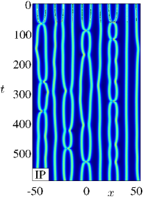
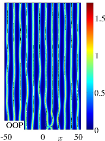
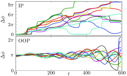
Figure 1: Color online. Dynamics of a slightly perturbed equidistant chain of 12 BSs of amplitude $a_{i}=1$ in the periodic domain $x\in[-54,54]$, namely a separation of $r_{0}=9$. The top left and right panels depict, respectively, the spatio-temporal evolution of the (square root of the) density $|u(x,t)|$ for the IP and OOP initial chains. The initial conditions are set as the numerically exact steady states found by Newton iterations and then the BSs positions are perturbed with randomly distributed displacements between $-r_{0}/18$ and $r_{0}/18$. The dashed lines represents the orbits obtained from the corresponding reduced Toda lattice model (9) (for the IP case this model can only be integrated until the first collision time for $t\lesssim 50$). The bottom two panels depict the phase difference between consecutive density maxima. These correspond to the relative phases $\Delta\phi$ between consecutive BSs (top and bottom subpanels corresponding, respectively, to the IP and OOP cases).

Since we are interested in excitations of the homogeneous chain, let us first study their stability. In Fig. 1, we depict typical time evolutions corresponding to an IP (top-left) and OOP (top-right) BS chain. The system is initialized using the numerical steady state of the GP system with periodic boundary conditions —found using a standard fixed point iteration algorithm— with a small perturbation. As can be seen in the figure, both the IP and OOP cases are unstable. The nature of the instability seems, however, different. The IP case, for which we know that even in the reduced ODE model is unstable due to the mutual attraction between BSs, seems to be strongly unstable. The instability is manifested by two neighboring BS coalescing as early as $t\approx 50$. This instability is easy to understand since a small perturbation will induce two neighboring BSs to be slightly closer than its other neighbors, thus accelerating the process of attraction and hence leading to a rapid collision between these two BSs. On the other hand, in the OOP case, the reduced chain is neutrally stable and, thus, perturbations with respect to the positions of the BSs from the equidistant chain should not cause instabilities. As shown in the top-right panel of Fig. 1, this is the case for intermediate times ($t<500$) where the mutual repulsion between BSs is responsible for collision avoidance between neighboring BSs. Nonetheless, as the panel shows, for later times, $t\approx 575$, a collision between neighboring BSs does indeed occur. The presence of a collision is unequivocal evidence that the involved BSs where not OOP when they collided. In fact, the loss of the OOP property between consecutive BSs is precisely what induces the instability of the otherwise OOP initial BS chain. The desynchronization between the phases can be clearly seen in the bottom two subpanels of Fig. 1. The panels depict the time evolution of the relative phase between consecutive BSs that initially start in the IP (top subpanel) and the OOP (bottom subpanel) configurations. It is clear that the OOP property between consecutive BSs is approximately held for intermediate times (see $t<500$ in the bottom subpanel) ensuring the mutual repulsion between consecutive BSs and, thus, stability for the chain. However, it is also clear that the OOP property gets progressively worse until a pair of consecutive BSs have a zero relative phase between them, i.e. they are IP around $t=575$, inexorably leading to their collision.

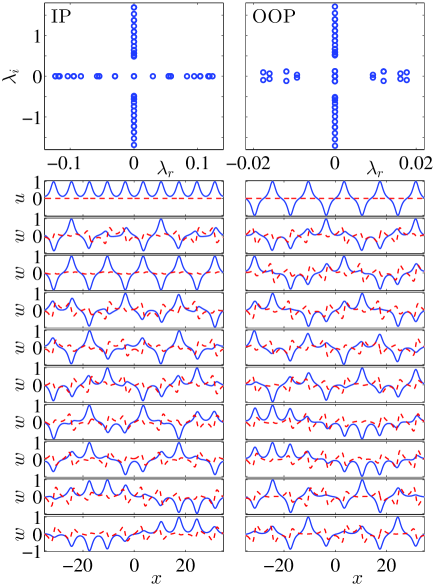
Figure 2: Color online. BdG stability spectrum for the steady state for a chain of 10 equidistant chain of IP (top left) and OOP (top right) BSs in the periodic domain $x\in[-35,35]$. The bottom set of panels depict, from top to bottom, the steady state and the first nine most unstable eigenfunctions where the real part is depicted by the (blue) solid line and the imaginary part by the (red) dashed line.

To further understand the nature of the instability, we have computed the Bogolyubov-de Gennes (BdG) stability spectrum for the IP and OOP steady states of the GP system. The BdG spectrum is computed by considering perturbations from the steady state $u_{0}(x)$ of the following form:

$$u(x,t)=\left(u_{0}(x)+\varepsilon(a(x)e^{\lambda t}+b(x)e^{-\lambda^{*}t})\right)e^{-i\mu t},$$ (8)

where $\mu$ is the so-called chemical potential (or [the negative of] the temporal frequency) of the solution, $\lambda$ is the eigenvalue with associated eigenvector $\{a,b^{*}\}$, and where $(\cdot)^{*}$ stands for complex conjugation. After applying the perturbation ansatz (8) into the GP equation (1) and linearizing the ensuing equation, one obtains an eigenvalue problem with a corresponding eigenfunction $w(x)=a(x)+b^{*}(x)$ at $t=0$. After computing the spectrum, any eigenvalue $\lambda=\lambda_{r}+i\lambda_{i}$ with a positive real part ($\lambda_{r}$) indicates an unstable eigenfunction. The spectrum associated with the IP and OOP steady states is depicted, respectively, in the left and right top panels of Fig. 2. As is can be noticed, the OOP spectrum has a handful of complex eigenvalues with a small ($\lambda_{r}<0.02$) real part indicating a weak instability. In contrast, the IP case reveals a larger (purely real) instability with $\max(\lambda_{r})\approx 0.123$, indicating a stronger instability. Closer inspection of the unstable eigenfunctions (see bottom set of panels in Fig. 2) reveals that the instabilities manifest themselves as local translational modes for consecutive BSs in the opposite direction and, thus, bringing them closer to each other. We have checked that the stability results above (cf. Figs. 1 and 2) are very similar for other values of the parameters such as amplitude, number, and separation of the BSs, as well as different domain lengths. Evidently, as more BSs are included in the system, a higher degeneracy of the eigenvalues arises since all solutions and eigenfunctions posses translational symmetry. Finally, it is relevant to mention that the BS chain might be rendered stable by a suitable choice of periodic lattice potential providing stabilizing pinning for each BS located at the respective minimum of the lattice potential pre-foc ; bec-pra . However, we do not explore this avenue further in this manuscript.

Since the IP BS chain is highly unstable, we will focus our attention in the case of the weakly unstable OOP chain. Therefore, let us consider the case $\sigma_{i,j}=+1$ for which the reduced equation of motion yields

$$\ddot{\xi}_{i}=4a^{3}\,e^{-a(\xi_{i}-\xi_{i-1})}-4a^{3}\,e^{-a(\xi_{i+1}-\xi_{i})},$$ (9)

which has precisely the form of the celebrated Toda lattice Toda_book that is further described below. It is important to mention at this stage that the restriction of locked phases between BSs (IP or OOP) is not necessary to obtain a Toda lattice-type model. In fact, by allowing the phase of each BS to dynamically evolve, the equations of motion (5) reduce to a complex Toda lattice of the form Gerdjikov:97 :

$${\ddot{q}_{j}}=2a\,\left(e^{-(q_{j}-q_{j-1})}-e^{-(q_{j+1}-q_{j})}\right),$$ (10)

where the corresponding complex variable $q_{j}$ for this complex Toda lattice is defined through the original BS’s parameters by

$$q_{j}=a\,\xi_{j}-j\,\ln{(a^{2})}+i\,\left(j\,\pi-v\xi_{j}+\delta_{j}+\delta\right),$$ (11)

where $a$ and $v$ are the ensemble average height and velocity of the BSs, while $\xi_{j}$ is the position of the $j$-th BS and the $\delta_{j}$’s are the BS phases and $\delta$ is their average.

II.2 Dark soliton chains

As was done in the previous section for the BS chain, the case of DS chains can also be reduced to a set of ODEs on the DS parameters. This reduction is obtained through DS perturbation theory as described in detail in Refs. Kivshar_BAM_1989 ; Kivshar_Pang_94 ; Kivshar_Krol_95 ; DJF_REVIEW ; DARK_BOOK . In particular, considering a DS ansatz of the form (3) for all DSs in a chain supported on a constant background with density $n_{0}$, the equations of motion are approximately reduced to

$$\ddot{\xi}_{i}=8n_{0}^{3/2}\,e^{-2\sqrt{n_{0}}(\xi_{i}-\xi_{i-1})}-8n_{0}^{3/2}\,e^{-2\sqrt{n_{0}}(\xi_{i+1}-\xi_{i})},$$ (12)

which, as for the BS chain, is a form of the Toda lattice Toda_book on the DS positions.

The main difference between the reduced dynamics of bright and dark solitons that is worth pointing at this stage is that BSs can have mutual interactions that are repulsive or attractive depending on their relative phases as described above. On the other hand, DSs are always repulsive. Therefore, the stationary homogeneous, equidistant, DS chain is always stable. This observation will be crucial when comparing the dynamics of BS and DS chains from the GP model (1) and their respective dynamical reductions (7) and (12).

II.3 Validation of the Toda lattice reduction

We now validate the dynamics obtained from the dynamical reduction for both bright and dark soliton chains. In order to numerically approximate an infinite lattice, we take a periodic domain in the interval $x\in[-L,L]$ and place the solitons equidistant from each other accounting for the periodic boundary conditions. Thus, considering $N$ solitons gives a steady state equidistant configuration such that $|\xi_{i+1}-\xi_{i}|=r_{0}$ for $i=1,\dots,N-1$, where the distance $|\cdot|$ is measured in the periodic domain such that $|\xi_{N}-\xi_{1}|=2L-r_{0}$.

Let us first consider a BS chain. As we described earlier, the perturbed equidistant chain evolves as depicted in Fig. 1 where the top left and right panels correspond, respectively, to the IP and OOP cases. We have superimposed the corresponding dynamics of the reduced ODE model of the BSs (9) using dashed lines. As can be observed from the figure, in the IP case (top left panel) before the collision of the BSs ($t<50$), the ODE model very closely follows the BS dynamics. After collision, the ODE model breaks down as the BS centers coalesce and, thus, we only show the reduced ODE orbit up to the first collision time. On the other hand, for intermediate times, the OOP chain (top right panel) does not suffer from the collision of BSs as it assumes that all BSs are always OOP. The resulting reduced ODE dynamics closely follows the original GP dynamics for short times, but later deteriorates since, as explained earlier, the BSs lose the OOP synchronization. Nonetheless, for intermediate times, while the BSs are kept separated, the reduced ODE model does reproduce the original GP dynamics.

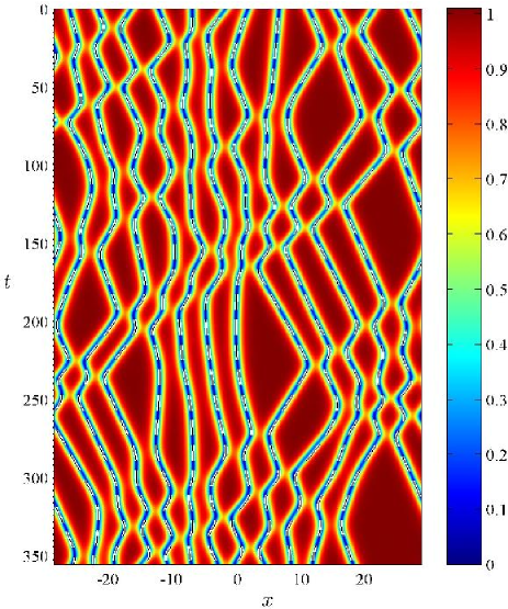
Figure 3: Color online. Interaction dynamics for 12 DSs initialized at random positions with random velocities in a periodic domain. Depicted is the spatio-temporal evolution of the (square root of the) density. The dashed lines represent the orbits obtained from the corresponding reduced Toda lattice model (12).

In contrast to the BS chain, the DS chain does not suffer from phase-induced instabilities since DSs always repel each other. As a result, the reduced ODE model for the DS chain (12) provides a very robust model for the GP dynamics under extended time evolutions for any initial condition provided the DSs are initially well-separated. An example of the dynamics from the reduced Toda lattice ODE (12) and the original GP model is depicted in Fig. 3, where a collection of DSs placed at random locations with random initial velocities evolves in time. It is clear from the figure that the Toda lattice model gives an accurate prediction of the DS positions for the original GP system for long times.

III Toda lattice solitons

III.1 Preliminaries

Before constructing Toda lattice solitons on the chains of bright and dark solitons, let us review the form of these solutions for completeness. The Toda lattice is one of the most popular models in physics since, by construction, it was designed as to prescribe a chain of nonlinear oscillators with completely integrable evolution Toda_book . As such, the Toda lattice possesses some exact solutions that are the foundation for building more complex solutions. In particular, the Toda lattice possesses periodic and localized solutions Toda_book . Here we focus on the latter type of solutions referred to as Toda solitons. The Toda lattice’s equations of motion

$$\begin{array}[]{rcl}\ddot{y}_{n}&=&V_{\rm TL}(y_{n+1}-y_{n})-V_{\rm TL}(y_{n}-y_{n-1}),\\[8.61108pt] &=&A\,e^{-b(y_{n}-y_{n-1})}-A\,e^{-b(y_{n+1}-y_{n})},\end{array}$$ (13)

originate from the interaction of nearest neighbors in a one-dimensional chain of coupled, unit mass, particles at positions $y_{n}$, interacting through the potential

$$V_{\rm TL}(\Delta y)=\frac{A}{b}e^{-b\,\Delta y}+A\,\Delta y.$$ (14)

Here, $\Delta y$ is the separation between particles and $A$ and $b$ are positive parameters prescribing, respectively, the strength and decay of the inter-particle interactions. By following the evolution of the particles through their mutual separation

$$\Delta y_{n}=y_{n+1}-y_{n},$$ (15)

and defining $s_{n}\equiv d({{\Delta y}}_{n})/dt$ and $p_{n}\equiv dy_{n}/dt$ so that $s_{n-1}-s_{n}=p_{n}$, the equations of motion can be rewritten in term of $S_{n}=\int s_{n}dt$ as

$$\ln\left(1+\frac{\ddot{S}_{n}}{a}\right)=\frac{b}{m}\left(S_{n+1}-2S_{n}+S_{n-1}\right).$$ (16)

Then, it is straightforward to find solitary kink solutions for this system in the form:

$$s_{n}=\pm\frac{\beta}{b}\tanh\left(n\kappa\pm\beta t\right)+{\rm const},$$ (17)

where the kink velocity is $c=\beta/\kappa$ and its amplitude $\beta$ is given by

$$\beta=\displaystyle\sqrt{Ab}\,\sinh\kappa,$$ (18)

where the width of the kink $\kappa$ is a free parameter. It should be noticed that this solution is stable and it corresponds to a compression wave that travels through the lattice Toda_book .

III.2 Toda lattice solitons: hypersolitons

We now seek to use the soliton solution for the Toda lattice (see previous section) to construct a Toda lattice soliton on the reduced lattice equations for the bright and dark soliton chains. Let us consider an equilibrium configuration consisting of a chain of $N$ equidistant solitons with separation $r_{0}=2L/N$ in the periodic domain $x\in[-L,L]$. Both OOP BS and DS chains are reduced, respectively, to the Toda lattice chains (9) and (12) where the Toda lattice potential parameters are given in terms of soliton amplitude $a$ for the BS chain and in terms of the background density $n_{0}$ for the DS chain. It is worth mentioning that the uniform pre-compression experienced by the periodic chain effectively corresponds to a rescaling on the strength of the Toda lattice potential $A$. This is evident when rescaling the soliton positions by a factor $\gamma$, $y_{n}=\gamma\tilde{y}_{n}$, then the exponential interaction terms become $A\,e^{-b(y_{n}-y_{n-1})}=A\,e^{-b\gamma(\tilde{y}_{n}-\tilde{y}_{n-1})}=\tilde{A}\,e^{-b(\tilde{y}_{n}-\tilde{y}_{n-1})}$ where $\tilde{A}=A\,e^{-b\gamma}$.

Let us start by initializing the chain of BSs such that the initial positions and initial velocities satisfy the corresponding Toda soliton (17). An example of this case is depicted in Fig. 4 for $N=10$ BSs in the periodic chain $x\in[-43,43]$. The top panels depict the initial condition for the displacements from equilibrium between solitons $r_{n}=\xi_{n}-\xi_{n-1}-r_{0}$ (left subpanel) and their respective initial velocities ${\dot{r}}_{n}$. As it is evident from these panels, the kink (17) corresponds to a localized compression wave for the soliton’s positions. It is worth mentioning at this stage that contrary to the homogeneous, equidistant, chain where $2L=N\,r_{0}$, for the chain initialized with the Toda lattice solitons the length of the domain has to be adjusted since we are introducing a compression wave to the initial condition. Thus, we compute the length of the domain by adding all the separations between consecutive solitons. The bottom row of panels in Fig. 4 depicts the evolution of the density after seeding the original GP equation with the Toda lattice soliton initial conditions on a pre-compressed BS chain. As it can be observed from the left subpanel, the initialized compression wave travels at the prescribed speed —for this panel we set the final time to precisely $2c/(2L)$, namely, the time needed to perform exactly two complete cycles through the lattice. In the figure, the dashed lines correspond to the Toda lattice soliton from the reduced ODE model (9) which, for short times, accurately approximates the full GP dynamics. However, as we have described before, the BSs will eventually lose their OOP synchronization leading to the coalescence of two consecutive solitons. The first coalescence occurs approximately at $t=125$ for the right-most two solitons of the lattice. Nonetheless, after this coalescence, the Toda lattice soliton seems to reform again which, in turn, suffers from the coalescence of more BSs as time progresses. It is interesting to note that although the reduced ODE should fail after a BS pair loses its OOP synchronization, and as it was noted in Ref. Gerdjikov:97 , for OOP initial conditions, the reduced ODE model still captures the dynamics of the interacting chain for some time. Nonetheless, as can be seen in the bottom right panel of Fig. 4, after longer integration times (10 full cycles around the lattice), the Toda soliton does not preserve its shape and other excitations start populating the dynamics, including Toda solitons that apparently move in the opposite direction of the original Toda soliton. By the same token, it is also evident that the ODE description (see dashed line) fails to capture the long term dynamics of the original GP system. This is evidence that the unstable character of the BS chain due to the desynchronization of the phases precludes satisfactory modeling of the full GP system with the reduced ODE (9) where all BSs are assumed to be OOP.

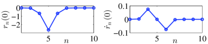
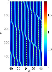
Figure 4: Color online. Toda lattice soliton riding on a chain of $N=10$ BSs in the periodic domain $x\in[-43,43]$. The top panels depict the initial conditions in terms of the relative displacements from equilibrium $r_{n}(t=0)$ (left subpanel) and their corresponding velocities $\dot{r}_{n}(t=0)$ (right subpanel). The bottom left and right panels depict the evolution of the (square root of the) density of the original GP model initialized with the Toda lattice soliton for, respectively, a total time equivalent to two and ten cycles of the Toda lattice soliton around the periodic domain. The dashed lines correspond to the reduced ODE model of the Toda lattice (9).

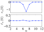
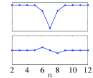
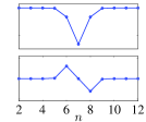
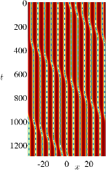
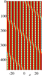
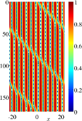
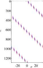
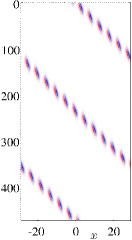
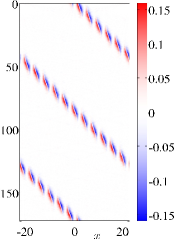
Figure 5: Color online. Toda lattice soliton riding in a chain of $N=12$ DSs on a periodic domain. The top two rows of panels depict the initial conditions in terms of the relative displacement from equilibrium of the mutual distances $r_{n}(0)$ (top subpanels) and their corresponding velocities (bottom subpanels). The middle and bottom row of panels depict, respectively, the evolution of the (square root of the) density $|u(x,t)|$ and its time derivative for the original GP model initialized with the Toda lattice soliton. The left, middle and right columns correspond to increasingly large Toda lattice velocities for a background density $n_{0}=1$ and, from left to right, $r_{0}=6$, $r_{0}=5$, and $r_{0}=4$, which correspond, respectively, to $c=0.0180$, $c=0.0489$, and $c=0.1329$. The dashed lines correspond to the reduced ODE model of the Toda lattice (12).

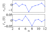
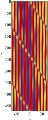
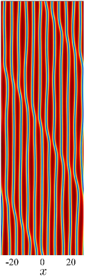
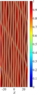
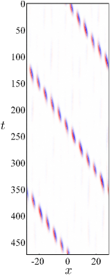
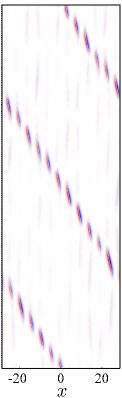
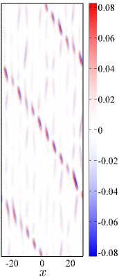
Figure 6: Color online. Stability of the hypersoliton. The layout of the different panels is the same as in Fig. 5. The initial condition corresponds to the case of the middle column of panels of Fig. 5 ($r_{0}=5$) with random perturbations added to the initial condition. The initial condition is perturbed by adding a random perturbation of size, from left to right, 30%, 50%, and 80% on the initial separations and velocities of the DSs in the chain.

Let us now turn our attention to the DS case. Here, the problem of the desynchronization of the phases is naturally avoided and thus it should be possible to observe Toda solitons travelling stably through the DS chain. In fact, this is precisely what we observe in our numerics for a wide range of parameters for the DSs themselves and of the Toda soliton. Figure 5 depicts three of such examples corresponding to three difference Toda soliton initial velocities. The different velocities are computed from the Toda lattice soliton solution (17) corresponding to the reduced Toda model for the DSs (12) for $n_{0}=1$ and unperturbed initial separations $r_{0}=6$, 5, and 4. The top panels in the figure depict the initial compression wave ($r_{n}$) and its initial velocity ($\dot{r}_{n}$). The middle row of panels depicts the dynamics on the (square root of the) density ($|u|$) together with the reduced ODE Toda model (12) superimposed to it. The bottom row of panels depicts the time derivative of the (square root of the) density ($|u|_{t}$) illustrating that outside of the region of localization of the Toda soliton, there are no perturbations indicating a stable, radiationless, propagation of the Toda soliton. From now on, we dub such a solution a hypersoliton as it is a (Toda lattice) soliton riding on a chain of (dark) solitons. As shown in Fig. 5, the reduced Toda lattice and, in particular, its Toda lattice solution, accurately describes the behavior of the original GP model.

In order to further study the stability and robustness of the crafted hypersolitons, we proceed to initialize the lattice with an initial condition corresponding to a perturbed hypersoliton. Specifically, Fig. 6 shows the dynamical evolution after using 30%, 50%, and 80% random initial perturbations to, both, initial relative positions and their respective velocities. It is remarkable that the addition of such high levels of perturbations to the initial conditions do not destroy the hypersoliton. Instead, these perturbation seem to just provide some background noise over which the hypersoliton rides with minimal interaction. This background noise is more clearly visible in the bottom row of panels depicting the time derivative of the (square root of the) density. This remarkable robustness of the hypersoliton even after the addition of such large perturbations to the initial conditions —that in turn develop into perturbations along the whole domain— is due to two independent facts: (a) on the one hand, DSs for the GP equation are very robust, a property owing from their topological charge, and (b) the structural stability of Toda solitons of the Toda lattice. These two stability properties, at two distinct levels of the model, combine to give the hypersoliton on the original GP model its robustness.

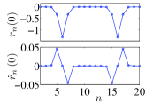
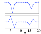
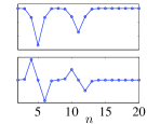
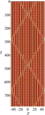
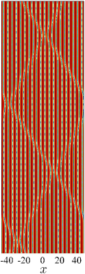
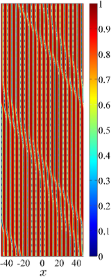
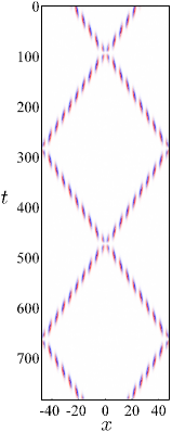
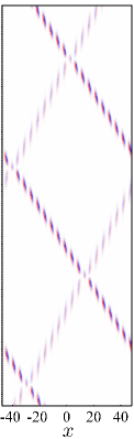
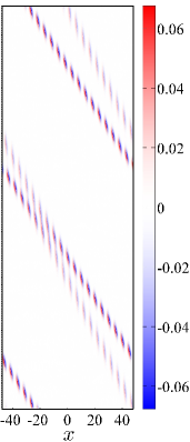
Figure 7: Color online. Hypersoliton collisions. The left, middle and right columns depict, respectively, the collision for (a) a head-on collision with equal but opposite velocities, (b) a head-on collision with different speeds, and (c) a chasing collision where a faster hypersoliton (seeded on the left) chases a slower hypersoliton (seeded on the right) until they collide in a nonlinear fashion. All panels have the same meaning and layout as previous figures.

III.3 Toda lattice solitons: hypersoliton collisions

Now that we have established the existence and stability of the hypersoliton solutions in DS chains, it is possible to study several dynamical aspects arising at this higher structural level. For example, one can initialize the DS chain with two (or more) hypersolitons and allow them to interact. It is expected that the dynamics governing the interactions between hypersolitons will be prescribed by the corresponding dynamics on the Toda lattice. In particular, Toda lattice solitons collide elastically without energy loss during the collision process. This is precisely what we observe for a wide range of cases when seeding two hypersolitons at different locations with different initial speeds (if they have the same velocity they will chase each other indefinitely). Figure 7 shows typical examples of hypersoliton collisions. Specifically, the left, middle and right cases correspond, respectively to: (a) a head-on collision for opposite velocities with the same magnitude, (b) a head-on collision for velocities with different magnitudes, and (c) two chasing hypersolitons where a faster one chases a slower one until they collide. As the bottom panels show, all these collisions, as expected, are elastic (i.e., no energy is lost from the travelling hypersolitons before or after the collisions). It is interesting to note, as per the “particle” nature of the hypersoliton structures, owed to their nonlinear character, there is a shift in their paths when comparing their straight line trajectories [in the $(x,t)$ plane] before and after collision. This effect is clearly visible in the last case of Fig. 7 where the fast soliton is advanced after collision while the slow one is delayed after collision. This effect will be important as we construct a quantum analog of the classical Newton’s cradle using hypersolitons in a chain of DS trapped inside a confining potential in the next section.

III.4 Quantum Newton’s cradle

We now proceed to study the effects of adding a confining external potential [i.e., $V_{\rm MT}\not=0$ in Eq. (1)], relevant to the modelling of magnetically trapped BECs, on the dynamics of hypersolitons supported by a finite DS chain. In the presence of the external parabolic potential (4), a single DS exhibits approximately harmonic oscillations with a frequency $\omega=\Omega/\sqrt{2}$ (see Refs. DJF_REVIEW ; DARK_BOOK ; pelpan ; fr4 ; fr5 and references therein). This result is valid in the so-called Thomas-Fermi limit corresponding to the high density limit. Therefore, combining —through perturbation theory— the mutual interactions between DSs and the force exerted by the external trap yields DJF_REVIEW ; DARK_BOOK

$$\ddot{\xi}_{i}=8n_{0}^{3/2}\,e^{-2\sqrt{n_{0}}(\xi_{i}-\xi_{i-1})}-8n_{0}^{3/2}\,e^{-2\sqrt{n_{0}}(\xi_{i+1}-\xi_{i})}-\omega^{2}\xi_{i},$$ (19)

corresponding to the Toda lattice described by Eq. (12) with an added on-site force generated by the external potential on each of the DSs of the chain. The above model has not only been validated numerically, but it has been used to predict the normal modes of vibration for a small number of DSs in actual experiments kip ; kip2 . In fact, the Toda lattice with the on-site potential (19) possesses a steady state solution emerging from the balance of the mutual repulsions between the DSs and the attraction of the external trap towards the trap’s center. This compressed steady state train of $N$ DSs has $N$ distinct normal modes of vibration corresponding to the normal modes of vibration of $N$ coupled masses through (linear) springs with springs at each end attached to rigid walls. For example, for $N=2$ there exist 2 normal modes of vibration corresponding to the in-phase and out-of-phase modes of vibration of the DSs kip2 .

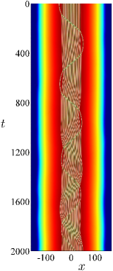
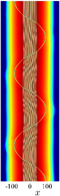
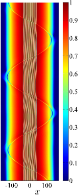
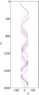
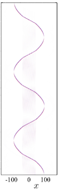
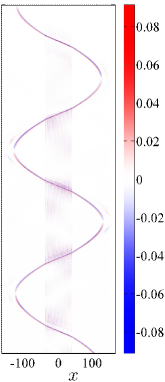
Figure 8: Color online. Hypersoliton Newton’s cradle. A DS soliton (leftmost one) is released at various distances away from a stationary lattice of 12 DSs placed at the center of the parabolic trapping potential (4) with $\Omega=0.01$. The DS is released at a distance equivalent to (a) $3r_{0}$ (left column of panels), (b) $12r_{0}$ (middle column of panels), and (c) $20r_{0}$ (right column of panels) where $r_{0}$ is the separation between the central DSs. All panels have the same meaning and layout as previous figures.

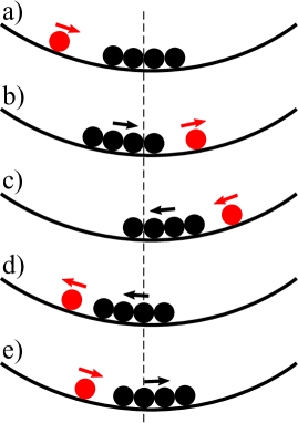
Figure 9: Color online. Schematic of the mechanism for the loss of the hypersoliton Newton’s cradle through the synchronization of the outer DS (red) with the central DS chain (black). (a) Release of a DS from the left with a stationary DS chain in the central region. (b) After the hypersoliton travels through the chain, the rightmost DS is ejected to the right. The remaining central DS chain is now asymmetric with respect to the center (see vertical dashed line) and starts moving to the right. (c) Both outer DS and central DS chain perform half an oscillation after their respective excursion up the trap. (d) After the DS collides and transfers its energy (through a propagating hypersoliton through the central DS chain) the leftmost DS is ejected. The central DS chain still has the extra energy of moving towards the left. (e) Both the DS and the central chain now oscillate in the same direction (although slightly out-of-phase). This process continues until the energy of the outer DS is completely transferred to the central chain and all that remains is a central chain undergoing left-to-right oscillations in the in-phase normal mode.

Instead of studying further the normal modes mentioned above, we opt here to emulate the dynamics of a classical Newton’s cradle using a chain of solitons. The idea is to start with an initial stationary chain of $N$ DSs at the bottom of the parabolic trap and then drop a single, outer, DS from a position higher up in the trapping potential. This outer DS will experience the force of the trapping potential and ride down the external trap to collide with the stationary DS chain. The collision excites a moving hypersoliton within the inner DS chain. When the hypersoliton reaches the opposite extreme of the inner DS chain, a single DS is expelled outward. This new outer DS will ride up and down the trap until it hits the inner DS chain thus repeating the process of a soliton analogue of the classical Newton’s cradle. It is relevant to note at this stage that a similar idea was experimentally achieved in a 1D Bose gas of ⁸⁷Rb atoms by initially splitting a wavepacket into two wavepackets with opposite velocities. These packets then evolve by going up and down the trap and periodically colliding at the center Cradle_Nature . Also, in Ref. Franzosi_14 , the authors propose another quantum analogue of a Newton’s cradle using a BEC by partitioning the wavefunction using a periodic optical lattice potential. In contrast, our method to create a Newton’s cradle is based on the effective nonlinearity of the GP model and the repulsive interaction dynamics between dark solitons.

Figure 8 depicts three different attempts at recreating a Newton’s cradle-type evolution with our setup. In these examples, we use a stationary DS chain of $N=12$ DSs placed at the center of a magnetic trap of strength $\Omega=0.01$, namely $\omega=0.01/\sqrt{2}$ [see Eq. (19)]. The stationary inner DS chain is obtained by a fixed-point iteration (Newton’s) method initialized with a chain of DSs with zero velocities positioned at the steady state locations. Once the stationary inner lattice is found, an extra, outer, DS is seeded away from it. The distance of the outer DS to the inner DS chain is varied and the resulting evolution is analyzed. The three cases depicted in Fig. 8 correspond to, from left to right, an initial distance of the outer DS of (a) $3r_{0}$, (b) $12r_{0}$, and (c) $20r_{0}$ where $r_{0}$ is the distance between the two innermost DSs of the central chain. For case (a), corresponding to a short dropping distance of the DS, the Newton’s cradle dynamics is observed for a couple of periods but apparently the outer DS is “absorbed” by the inner chain resulting in a larger inner chain (i.e., $N+1$ DSs) that simply oscillates in the in-phase normal mode. The mechanism whereby the outer DS is absorbed by the inner lattice hinges on the fact that, although DS collision are elastic, there is a shift in the path of the DSs with respect to the before and after collision trajectories as was shown before (see discussion on the last collision depicted in Fig. 7). The details of the outer DS “absorption”, or rather the energy exchange between the outer DS dynamics and the inner DS chain, is explained in Fig. 9. This energy transfer is more clearly visible in the left-bottom panel of Fig. 8 depicting the time derivative of the (square root of the) density. In this panel, it is clear that during the first hypersoliton excursion through the inner DS chain, there is practically no scattering of energy in the inner chain. However, as explained in Fig. 9, just after the hypersoliton ejects the first DS, the inner chain has an extra DS on the left and is missing one DS on the right and thus, it is no longer close to equilibrium and starts to oscillate. This is clearly visible in the bottom-left panel of Fig. 8 for $300<t<500$ where the inner chain moves synchronously. This energy transfer mechanism continues until all the energy of the outer DS is completely depleted and the outer DS is absorbed by the inner lattice that oscillates with its in-phase normal mode (results not shown here).

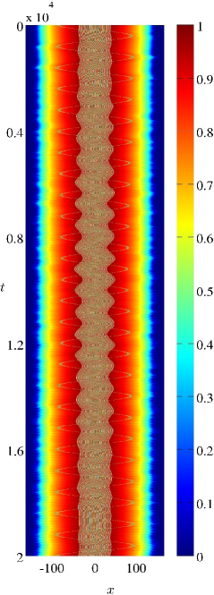
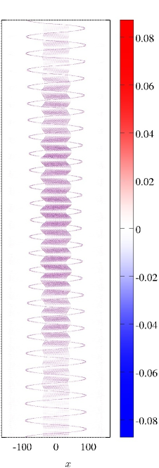
Figure 10: Color online. Long term evolution of the hypersoliton Newton’s cradle corresponding to the case depicted on the middle column of Fig. 8. Notice the beating of energy exchange between the outer DS and the central chain. All panels have the same meaning and layout as previous figures.

In order to avoid, or minimize, the energy transfer between the outer DS and the inner DS chain, it is necessary to decouple the dynamics of the outer DS and the inner DS chain. This is achieved by increasing the dropping distance of the outer DS. As can be seen in the case depicted in the middle column of panels in Fig. 8, the excursion of the outer DS has very little effect on the inner chain motion. This can be explained because in this case, the outer DS travels faster through the inner chain and thus, the latter has less time to develop its in-phase normal mode. Furthermore, as the period of the outer DS is different from the period of the inner chain in-phase mode, subsequent excursions of the outer DS do not synchronize with the in-phase mode. The outer DS has a different period in the presence of the inner DS chain because its trajectory in $(x,t)$ is the concatenation of sinusoids (when the outer DS is traveling up and down the external trap on its own) and straight paths (when the hypersoliton traverses the inner chain). Therefore, let us effectively consider the two involved dynamics, namely the outer soliton oscillations and the inner chain oscillations, as two coupled oscillators. These oscillators can synchronize provided that their periods are close to each other and that the coupling is sufficiently strong Strogatz:book . This is precisely what happens for a relatively small dropping distance as depicted in the first case of Fig. 8. However, as we increase the dropping distance, the two coupled oscillators have increasingly different frequencies and, at the same time, the coupling is reduced as the interaction time between the two, given by the time it takes for the hypersoliton to traverse the inner chain, is reduced because of a faster hypersoliton speed. Thus, in principle, there should be a threshold drop-off distance for which the Newton’s cradle should be self-maintained. This is what seems to be occurring in the case depicted in the middle column of Fig. 8 where apparently a very small amount of energy is transferred to the inner chain. To ensure that this small transfer does not destroy the Newton’s cradle, we depict in Fig. 10 the same case as in the middle column of Fig. 8, but for a longer time. As can be seen from the figure, there is indeed a transfer of energy from the outer DS to the inner chain for $t<9,000$. However, the roles are inverted after this time and then the inner chain transfers back the energy to the outer DS! This produces a beating phenomenon common for coupled oscillators with different periods. This periodic energy transfer between the outer DS and the inner chain seems to persists for very long times (results not shown here) providing a mechanism for a stable, long-lived, Newton’s cradle dynamics.

Finally, the last column of Fig. 8 depicts an example with an even larger drop-off distance. In this case, the outer DS also interacts with the edge of the BEC cloud and produces sounds waves that remove energy from the former and thus, finally settling to a Newton’s cradle with slightly lower oscillation amplitude with some background radiation (sound waves) prevailing in the condensate (results not shown here).

IV Conclusions and outlook

We construct coherent structures consisting of compression waves riding on chains of bright (BS) and dark (DS) solitons of the GP model. Namely, a soliton riding on a chain of solitons and thus dubbed a hypersoliton. The dynamics for chains of BSs and DSs is reduced to a Toda lattice on the solitons’ positions, i.e., the solitons are modelled as a chain of nonlinearly coupled masses. Then, the corresponding Toda lattice solitons (compression waves on the lattice) can be initialized on the original GP model using the exact Toda lattice soliton solution. We show how BS chains are inherently unstable due to phase desynchronization between consecutive BSs and thus are poor candidates for supporting hypersolitons. In contrast, DS chains are stable and DSs, being topologically charged, never lose their phases and thus are always mutually repelled from each other. We successfully craft hypersoliton solutions riding on DS chains of the original GP model for a wide range of parameter values. These hypersolitons are robust and stably travel at a constant speed without deformation nor radiation. Additionally, we construct multiple hypersolitons and observe their elastic collisions in different head-on and chasing collisions scenarios. Finally, inspired by the classical Newton’s cradle, we study the dynamics of finite DS chains trapped inside the customary parabolic external potential relevant in experimental Bose-Einstein condensates. This is achieved by letting a free, outer, soliton hit a stationary inner DS chain creating a hypersoliton wave travelling through the latter. As the hypersoliton reaches the end of the inner chain, a single DS is expelled and allowed to rise and fall down the external trap hitting the inner chain repeating the process in a manner akin to the classical Newton’s cradle. We study the effects of the drop-off distance on the formation of the Newton’s cradle dynamics and argue, in terms of the theory of coupled oscillators, that a minimal drop-off distance is required for the creation of self-sustained Newton’s cradle oscillations.

The present work could be extended in a few interesting directions. For example the effects of finite temperatures in a condensate give rise to dissipation due to coupling with the thermal (non condensed) fraction. This dissipation can be modelled at the level of the GP equation by the so-called phenomenological dissipation DJF_REVIEW ; DARK_BOOK and it is responsible for anti-damping terms in the reduced equations of motion of the DSs. It would be interesting to analyze the effects of such a dissipative term on the dynamics of hypersolitons. On the other hand, condensates can be supported by two or more coupled components with linear and/or nonlinear coupling terms between them BEC_BOOK . These coupled models give rise to coupled complexes with dark or bright solitons coupled to dark or bright solitons in the other component(s), thus giving rise to the so called dark-dark and dark-bright solitons pe2 ; pe3 ; pe4 ; pe5 . The dynamically reduced models for these coupled systems take the form of coupled Toda lattices Gerdjikov_TL_Manakov . It would be interesting to explore the possibility to construct hypersolitons and study their stability in systems with several components.

References

- (1) S.N. Bose. Zeitschrift für Physik 26 (1924) 178–181.
- (2) M.H. Anderson, J.R. Ensher, M.R. Matthews, C.E. Wieman, and E.A. Cornell. Science 269 (1995) 198–201.
- (3) K.B. Davis, M.-O. Mewes, M.R. Andrews, N.J. van Druten, D.S. Durfee, D M. Kurn, and W. Ketterle. Phys. Rev. Lett., 75 (1995) 3969–3973.
- (4) E.A. Cornell and C.E. Wieman. Rev. Mod. Phys., 74 (2002) 875–893.
- (5) P.G. Kevrekidis, D.J. Frantzeskakis, and R. Carretero-González (Eds.), Emergent Nonlinear Phenomena in Bose-Einstein Condensates: Theory and Experiment. Springer-Verlag, Heidelberg, 2008.
- (6) C.J. Pethick and H. Smith, Bose-Einstein Condensation in Dilute Gases. Cambridge University Press, Cambridge, 2001.
- (7) L.P. Pitaevskii and S. Stringari, Bose-Einstein Condensation. Oxford University Press, Oxford, 2003.
- (8) F. Dalfovo, S. Giorgini, L.P. Pitaevskii and S. Stringari. Rev. Mod. Phys, 71 (1999) 463.
- (9) K.E. Strecker, G.B. Partridge, A.G. Truscott, and R.G. Hulet, Nature, 417 (2002) 150–153.
- (10) L. Khaykovich, F. Schreck, G. Ferrari, T. Bourdel, J. Cubizolles, L.D. Carr, Y. Castin, and C. Salomon, Science, 296 (2002) 1290–1293.
- (11) S.L. Cornish, S.T. Thompson, and C.E. Wieman, Phys. Rev. Lett., 96 (2006) 170401.
- (12) S. Burger, K. Bongs, S. Dettmer, W. Ertmer, K. Sengstock, A. Sanpera, G.V. Shlyapnikov, and M. Lewenstein, Phys. Rev. Lett., 83 (1999) 5198–5201.
- (13) J. Denschlag, J.E. Simsarian, D.L. Feder, C.W. Clark, L.A. Collins, J. Cubizolles, L. Deng, E.W. Hagley, K. Helmerson, W.P. Reinhardt, S.L. Rolston, B.I. Schneider, and W.D. Phillips, Science, 287 (2000) 97–101.
- (14) Z. Dutton, M. Budde, C. Slowe, and L.V. Hau, Science, 293 (2001) 663–668.
- (15) B.P. Anderson, P.C. Haljan, C.A. Regal, D.L. Feder, L.A. Collins, C.W. Clark, and E.A. Cornell, Phys. Rev. Lett., 86 (2001) 2926–2929.
- (16) A.C. Scott. Nonlinear Science: Emergence & Dynamics of coherent structures (2nd. ed.), OUP, Oxford, 2003.
- (17) R. Carretero-González, D.J. Frantzeskakis, and P.G. Kevrekidis, Nonlinearity, 21 (2008) R139–R202.
- (18) D.J. Frantzeskakis, J. Phys. A: Math. Theor., 43 (2010) 213001.
- (19) P.G. Kevrekidis, D.J. Frantzeskakis, and R. Carretero-González, The Defocusing Nonlinear Schrödinger Equation: from Dark Solitons to Vortices and Vortex Rings. SIAM, 2015.
- (20) A.M. Kosevich, Physica D, 41 (1981) 253.
- (21) R. Scharf and A.R. Bishop, Phys. Rev. E, 47 (1993) 1375.
- (22) U. Al Khawaja, H.T.C. Stoof, R.G. Hulet, K.E. Strecker, and G.B. Partridge, Phys. Rev. Lett., 89 (2002) 200404.
- (23) P.G. Kevrekidis, D.J. Frantzeskakis, R. Carretero-González, B.A. Malomed, G. Herring, and A.R. Bishop, Phys. Rev. A, 71 (2005) 023614.
- (24) V.I. Karpman and V.V. Solov’ev. Physica D, 3 (1981) 142–164.
- (25) V.I. Karpman and V.V. Solov’ev. Physica D, 3 (1981) 487–502.
- (26) V.S. Gerdjikov, D.J. Kaup, I.M. Uzunov and E.G. Evstatiev. Phys. Rev. Lett., 77 (1996) 3943–3946.
- (27) V.S. Gerdjikov, I.M. Uzunov, E.G. Evstatiev and G.L. Diankov. Phys. Rev. E, 55 (1997) 6039–6060.
- (28) J.M. Arnold. J. Opt. Soc. Am. A, 15 (1998) 1450–1458.
- (29) J.M. Arnold. Phys. Rev. E, 60 (1999) 979–986.
- (30) R. Carretero-González and K. Promislow. Phys. Rev. A, 66 (2002) 033610.
- (31) J.C. Bronski, L.D. Carr, R. Carretero-González, B. Deconinck, J.N. Kutz and K. Promislow. Phys. Rev. E 64 (2001) 056615.
- (32) M. Toda. Theory of Nonlinear Lattices. Springer, Berlin, 1989.
- (33) Yu.S. Kivshar and B.A. Malomed Rev. Mod. Phys., 61 (1989) 763–915.
- (34) Yu.S. Kivshar and X.P. Yang. Phys. Rev. E, 49 (1994) 1657–1670.
- (35) Yu.S. Kivshar and W. Krolikowski. Opt. Commun., 114 (1995) 353–362.
- (36) D.E. Pelinovsky and P.G. Kevrekidis, Z. Angew. Math. Phys., 59 (2008) 559–599.
- (37) G. Theocharis, P. Schmelcher, M.K. Oberthaler, P.G. Kevrekidis, and D.J. Frantzeskakis, Phys. Rev. A, 72 (2005) 023609.
- (38) D.E. Pelinovsky, D.J. Frantzeskakis, and P.G. Kevrekidis, Phys. Rev. E, 72 (2005) 016615.
- (39) A. Weller, J.P. Ronzheimer, C. Gross, J. Esteve, M.K. Oberthaler, D.J. Frantzeskakis, G. Theocharis, and P.G. Kevrekidis, Phys. Rev. Lett., 101 (2008) 130401.
- (40) G. Theocharis, A. Weller, J.P. Ronzheimer, C. Gross, M.K. Oberthaler, P.G. Kevrekidis, and D. J. Frantzeskakis, Phys. Rev. A, 81 (2010) 063604.
- (41) T. Kinoshita, T. Wenger, and D.S. Weiss, Nature, 440 (2006) 900–903.
- (42) R. Franzosi and R. Vaia, J. Phys. B: At. Mol. Opt. Phys., 47 (2014) 095303.
- (43) S.H. Strogatz, Nonlinear Dynamics and Chaos (Perseus Books, Reading, MA, 1994).
- (44) S. Middelkamp, J.J. Chang, C. Hamner, R. Carretero-González, P.G. Kevrekidis, V. Achilleos, D.J. Frantzeskakis, P. Schmelcher, and P. Engels, Phys. Lett. A, 375 (2011) 642–646.
- (45) D. Yan, J.J. Chang, C. Hamner, P.G. Kevrekidis, P. Engels, V. Achilleos, D.J. Frantzeskakis, R. Carretero-González, and P. Schmelcher, Phys. Rev. A, 84 (2011) 053630.
- (46) M.A. Hoefer, J.J. Chang, C. Hamner, and P. Engels, Phys. Rev. A, 84 (2011) 041605(R).
- (47) D. Yan, J.J. Chang, C. Hamner, M. Hoefer, P.G. Kevrekidis, P. Engels, V. Achilleos, D.J. Frantzeskakis, and J. Cuevas, J. Phys. B: At. Mol. Opt. Phys., 45 (2012) 115301.
- (48) V.S. Gerdjikov, N.A. Kostov, E.V. Doktorov, and N.P. Matsuk, Math. Comput. Simulat., 80 (2009) 112–119.