Direct Adaptive Controller for Uncertain MIMO Dynamic Systems with Time-varying Delay and Dead-zone Inputs

Abstract

This paper presents an adaptive tracking control method for a class of nonlinearly parameterized MIMO dynamic systems with time-varying delay and unknown nonlinear dead-zone inputs. A new high dimensional integral Lyapunov-Krasovskii functional is introduced for the adaptive controller to guarantee global stability of the considered systems and also ensure convergence of the tracking errors to the origin. The proposed method provides an alternative to existing methods used for MIMO time-delay systems with dead-zone nonlinearities.

1 Introduction

In the past decades, control of multiple-input-multiple-output (MIMO) practical systems has attracted a great deal of attention, such as flying robots (Ge, Ren, Tee, and Lee (2009)), biped robots (Ge, Li, Yang (2011)) and underwater vehicle (Cui, Ge, How, Choo (2010)). To characterize certain non-sensitivity for small control inputs of these MIMO systems, dead-zone nonlinearities have to be considered otherwise it can severely limit system performances, even leading to instability. To handle dead-zone nonlinearities, many control approaches have been developed in the literature such as (Zhang, Ge (2007)) and (Chen, Liu, Lin (2013)). On the other hand, time-delay usually can be encountered in these MIMO systems, dealt with by many authors, e.g., (Cui, Ge, How, Choo (2010)) and references therein. Time-delay, like the dead-zone nonlinearities, can also degrade the system performances or lead to instability if ignored during the course of controller designs. Given the effects of the dead-zone and time-delay, this paper considers a class of nonlinearly parameterized MIMO dynamic systems where time-varying delay and unknown nonlinear dead-zone are simultaneously taken into accounts.

To the considered problem in this paper, the most relevant papers are (Zhang, Ge (2007)), (Chen, Liu, Lin (2013)), (Zhou (2008)), (Shyu, Liu, Hsu (2005)) and (Hua, Wang, Guan (2008)). In (Zhang, Ge (2007)), an adaptive neural control was proposed for a class of uncertain MIMO nonlinear state time-varying delay systems with unknown nonlinear dead-zones and gain signs, however, it only guarantees semiglobal stability of the closed-loop system. Both (Chen, Liu, Lin (2013)) and (Zhou (2008)) used the backstepping techniques to construct the controllers. However, the backstepping procedure is computationally time-consuming due to the computation of many virtual controllers for the MIMO systems. The authors of (Shyu, Liu, Hsu (2005)) proposed a decentralized controller for large-scale systems with time-delay and dead-zone nonlinearities. However, in (Shyu, Liu, Hsu (2005)), the time-delay is constant and the parameters of the dead-zone are known. In (Hua, Wang, Guan (2008)) the authors constructed a novel Lyapunov function and then designed a smooth adaptive state feedback controller for the time-delay system with dead-zone input. However, linear dead-zone was considered and the tracking error can converge only within an adjustable region. Thus one may wonder if it is possible to propose a new control method completely different from those existing ones to overcome these disadvantages mentioned above? This paper provides an affirmative answer by introducing a new high dimensional integral functional as a Lyapunov-Krasovskii function of the closed-loop systems.

From the motivation above and following our previous work (Ge, Li (2014)), this paper introduces a new high dimensional integral Lyapunov-Krasovskii functional for a class of nonlinearly parameterized MIMO systems with time-varying delay in states and unknown nonlinear dead-zones to achieve its tracking control.

Compared to the existing results, the main contributions of this paper are: i) By proposing a Lyapunov-based adaptive control structure, neither cancelation of the coupling matrix during linearizing the system nor conventional backstepping techniques is needed; ii) By introducing a new high-dimensional integral Lyapunov function in the control design, the process of controller design is simplified, i.e., it is unnecessary to calculate the inverse of the unknown control gain matrix; iii) By the construction of the Lyapunov-Krasovskii functional, the unknown time-varying delay in the upper bounding function of the Lyapunov functional derivative can be easily eliminated; iv) The developed control strategy is applied to a 2-DOF robotic manipulator system and the comparative simulation studies demonstrate the superiority of the proposed method.

2 Problem Statement and Assumptions

Consider the following uncertain MIMO nonlinear time-delay system with dead-zone nonlinearities

$$\left\{\begin{array}[]{ll}\dot{\mathbf{x}}_{i}=\mathbf{x}_{i+1},\\ \dot{\mathbf{x}}_{n}=\mathbf{B}^{-1}(\mathbf{x})\left[\mathbf{F}(\mathbf{x}(t-\tau(t)))+\mathbf{D}(t)+\mathbf{u}\right],\\ \mathbf{y}=\mathbf{x}_{1},\end{array}\right.$$ (4)

where $\mathbf{x}=[\mathbf{x}_{1}^{T},\mathbf{x}_{2}^{T},\dots,\mathbf{x}_{n}^{T}]^{T}\in\mathbb{R}^{nm}$ is the state vector, $\mathbf{x}_{i}=[x_{i1},x_{i2},\dots,x_{im}]^{T}\in\mathbb{R}^{m}$ and $\mathbf{y}^{(i-1)}=\mathbf{x}_{i}(i=1,2,\dots,n)$; the nonlinear function $\mathbf{F}(\mathbf{x}(t-\tau(t)))\in\mathbb{R}^{m}$; $\mathbf{B}(\mathbf{x})\in\mathbb{R}^{m\times m}$ are unknown continuous bounded function matrix; and the nonlinear function vector $\mathbf{D}(t)=[d_{1},d_{2}.\dots,d_{m}]^{T}$ denotes the external disturbance. $\mathbf{u}=[u_{1},u_{2},\dots,u_{m}]^{T}\in\mathbb{R}^{m}$ is the output of the dead-zone control input and satisfies that if $v_{i}\geq b_{ir}$, $u_{i}=g_{ir}(v_{i})$; if $b_{il}<v_{i}<b_{ir}$, $u_{i}=0$; if $v_{i}\leq b_{il}$, $u_{i}=g_{il}(v_{i})$, where $v_{i}\in\mathbb{R}$ is the input to the $i$th dead-zone, and $b_{il}$ and $b_{ir}$ are the unknown parameters of the $i$th dead-zone. In the paper, we consider the dimension of $\mathbf{y}$ and $\mathbf{x}_{i}(i=1,2,\dots,n)$ are equal, therefore, $\mathbf{y}=\mathbf{x}_{1}$ holds.

The control objective is to find a control input $V=[v_{1},v_{2},\dots,v_{m}]^{T}$ such that the output of the system tracks the desired trajectory $\mathbf{y}_{d}\in\mathbb{R}^{m}$ , while all the signals of the closed-loop system are globally bounded.

Remark 2.1.

The introduction of $\mathbf{B}(\mathbf{x})$ is for the physical meaning of mechanical system, which can represent to the inertia matrix for the system.

Remark 2.2.

The matrix $\mathbf{B}(\mathbf{x})\in\mathbb{R}^{m\times m}$ is known to be either uniformly symmetric positive definite or uniformly symmetric negative definite for all $\mathbf{x}\in\mathbb{R}^{n}$, and have $m$ eigenvalues. Therefore, for the positive definite case, we have the following inequalities

$$\lambda_{min}(\mathbf{B})\|x\|^{2}\leq x^{T}\mathbf{B}x\leq\lambda_{max}(\mathbf{B})\|x\|^{2},\quad\forall x\in\mathbb{R}^{n},$$

where $\lambda_{min}(\mathbf{B})$ and $\lambda_{max}(\mathbf{B})$ denote the minimum and maximum eigenvalues of $\mathbf{B}$, respectively (Li, Ge, Wang (2008)), (Li, Ding, Gao, Duan, Su (2013)).

Assumption 2.1.

(Zhang, Ge (2007)) The dead-zone outputs $u_{1},\ldots,u_{m}$ are not available and the dead-zone parameters $b_{ir}\mbox{ and }b_{il}$ are unknown constants, but their signs are known, i.e., $b_{ir}>0\mbox{ and }b_{il}<0,i=1,2,\ldots,m$. The growth of the $i$th dead-zone’s left and right functions, $g_{il}(v_{i})$ and $g_{ir}(v_{i})$, are smooth, and there exist unknown positive constants $k_{il0},k_{il1},k_{ir0}$ and $k_{ir1}$ such that

$$0<k_{il0} \leq g_{il}^{{}^{\prime}}(v_{i})\leq k_{il1},\quad\forall v_{i}\in(-\infty,b_{il}],$$ (5)

$$0<k_{ir0} \leq g_{ir}^{{}^{\prime}}(v_{i})\leq k_{ir1},\quad\forall v_{i}\in[b_{ir},+\infty),$$ (6)

where $\beta_{i0}\leq{\rm min}\{k_{il0},k_{ir0}\}$ is a known positive constant, and $g_{il}^{{}^{\prime}}(v_{i})={dg_{il}(z)}/{dz}|_{z=v_{i}}$ and $g_{ir}^{{}^{\prime}}(v_{i})={dg_{ir}(z)}/{dz}|_{z=v_{i}}$.

Assumption 2.2.

(Zhang, Ge (2008)) The unknown state time-varying delays $\tau_{i}(t)$ satisfy $\dot{\tau}_{i}(t)\leq\bar{\tau}_{max}<1$, $i=1,\cdots,m$, with the known constants $\bar{\tau}_{max}$.

We know that there exist (Zhang, Ge (2007)), $\xi_{il}(v_{i})\in(-\infty,b_{ir})$ and $\xi_{ir}(v_{i})\in(b_{il},+\infty)$ such that

$$g_{il}(v_{i}) = g_{il}(v_{i})-g_{il}(b_{il})=g_{il}^{{}^{\prime}}(\xi_{il}(v_{i}))(v_{i}-b_{il}),$$ (7)

$$\mbox{for}~{}~{}\xi_{il}(v_{i})\in(v_{i},b_{il})\mbox{ \rm or }(b_{il},v_{i}),$$

$$g_{ir}(v_{i}) = g_{ir}(v_{i})-g_{ir}(b_{ir})=g_{ir}^{{}^{\prime}}(\xi_{ir}(v_{i}))(v_{i}-b_{ir}),$$ (8)

$$\mbox{for}~{}~{}\xi_{ir}(v_{i})\in(v_{i},b_{ir})\mbox{ \rm or }(b_{ir},v_{i}).$$

Define vectors $\Phi_{i}(t)=[\varphi_{ir}(t),\varphi_{il}(t)]^{T}$ and $K_{i}(t)=[g_{ir}^{{}^{\prime}}(\xi_{ir}(v_{i}(t))),g_{il}^{{}^{\prime}}(\xi_{il}(v_{i}(t)))]^{T}$ with

$$\varphi_{ir}(t)=\left\{\begin{array}[]{lcl}1&\mbox{if}&v_{i}(t)>b_{il},\\ 0&\mbox{if}&v_{i}(t)\leq b_{il},\\ \end{array}\right.\ \varphi_{il}(t)=\left\{\begin{array}[]{lcl}1&\mbox{if}&v_{i}(t)<b_{ir},\\ 0&\mbox{if}&v_{i}(t)\geq b_{ir}.\\ \end{array}\right.$$

Based on Assumption 2.1, the dead-zone control input can be rewritten as follows

$$u_{i}=K_{i}^{T}(t)\Phi_{i}(t)v_{i}+\xi_{i}(v_{i}),$$ (9)

where

$$\xi_{i}(v_{i})=\left\{\begin{array}[]{lcl}-g_{ir}^{{}^{\prime}}(\xi_{ir}(v_{i}))b_{ir},&\mbox{if}&v_{i}\geq b_{ir},\\ -[g_{il}^{{}^{\prime}}(\xi_{il}(v_{i}))\\ +g_{ir}^{{}^{\prime}}(\xi_{ir}(v_{i}))]v_{i},&\mbox{if}&b_{il}<v_{i}<b_{ir},\\ -g_{il}^{{}^{\prime}}(\xi_{il}(v_{i}))b_{il},&\mbox{if}&v_{i}\leq b_{il},\\ \end{array}\right.$$ (10)

and $|{\xi_{i}(v_{i})}|\leq p_{i}^{\ast}$, where $p_{i}^{\ast}$ is an unknown positive constant with $p_{i}^{*}=(k_{ir1}+k_{kl1})\max\{b_{ir},-b_{il}\}$. Therefore, we have

$$\mathbf{u}=K^{T}\Phi V+\Xi,$$ (11)

where $K={\rm diag}[K_{i}(t)]$, $\Phi={\rm diag}[\Phi_{i}(t)]$ and $\Xi=[\xi_{1}(v_{1}),\dots,\xi_{m}(v_{m})]^{T}$.

Let $\mathbf{B}_{d}(\mathbf{x})\in\mathbb{R}^{m\times m}$ be a diagonal matrix with diagonal elements $b_{dii}\neq 0(i=1,2,\dots,m)$, then, there exists an unknown matrix $\Delta_{\mathbf{B}}$ such that $\mathbf{B}(\mathbf{x})=\mathbf{B}_{d}(\mathbf{x})+\Delta_{\mathbf{B}}$ is satisfied. We can rewrite (4) as

$$\mathbf{B}(\mathbf{x})\dot{\mathbf{x}}_{n}=\mathbf{F}(\mathbf{x}(t-\tau(t)))+\mathbf{D}(t)+\mathbf{u}.$$ (12)

Substituting (11) and $\mathbf{B}(\mathbf{x})$ into (12), we can obtain

$$\mathbf{B}_{d}(\mathbf{x})\dot{\mathbf{x}}_{n}=\mathcal{F}(\mathbf{x}(t-\tau(t)))+K^{T}\Phi V+\Delta_{P},$$ (13)

where

$$\mathcal{F}(\mathbf{x}(t-\tau(t))) = (I-\Delta_{\mathbf{B}}\mathbf{B}^{-1}(\mathbf{x}))\mathbf{F}(\mathbf{x}(t-\tau(t)))$$ (14)

$$= [f_{1},f_{2},\dots,f_{m}]^{T}$$

and

$$\Delta_{P}=-\Delta_{\mathbf{B}}\mathbf{B}^{-1}K^{T}\Phi V+(I-\Delta_{\mathbf{B}}\mathbf{B}^{-1})(\Xi+\mathbf{D})$$ (15)

are column vectors.

Assumption 2.3.

(Ge, Hang, Zhang (1999)) Functions $b_{dii}$ and $d_{i}$ are continuous unknown. $b_{dii}$ and $d_{i}$ respectively satisfy $b_{dii}=W_{Bii}^{T}\Phi_{Bii}(\mathbf{x})$ and $d_{i}\leq W_{di}^{T}\Phi_{di}(t)$ where $W_{Bii}\in\mathbb{R}^{l}$ is unknown bounded constant parameter vectors, $\Phi_{Bii}(\mathbf{x})\in\mathbb{R}^{l}$ is the known continuous smooth bounded regressor vector, $W_{di}\in\mathbb{R}^{l}$ is a vector of unknown bounded constant parameters, and $\Phi_{di}(t)\in\mathbb{R}^{l}$ is a vector of smooth bounded nonlinear function $\mathbf{x}$.

Assumption 2.4.

(Zhang, Ge (2008)) The unknown continuous functions $f_{1},f_{2},\ldots,f_{m}$ satisfy the inequality

$$|f_{i}|\leq\sum_{k=1}^{m}\varrho_{ik}(\mathbf{x}_{k}(t-\tau_{k}(t)))$$ (16)

with $\varrho_{ik}(x_{k}(t))(i=1,2,\dots,m)$ being known positive continuous functions.

Lemma 2.1.

(Ge, Lee, Harris (1998)) Let $H(s)$ denote an $(n\times m)$-dimensional exponentially stable transfer function, $r$ be the input and $e=H(s)r$ be the output. Then $r\in L_{2}^{m}\bigcap L_{\infty}^{m}$ indicates that $e,\dot{e}\in L_{2}^{n}\bigcap L_{\infty}^{n}$, $e$ is continuous, and $e\to 0$ as $t\to\infty$. Moreover, if $r\to 0$ as $t\to\infty$, then $\dot{e}\to 0$.

3 Control Design and Analysis

Define the filtered tracking error $s_{i}$ (Slotine, Li (1993))

$$s_{i} = e_{i}^{(n-1)}+\lambda_{i1}e_{i}^{(n-2)}+\dots+\lambda_{i,n-1}e_{i},$$ (17)

where $e_{i}=y_{i}-y_{di}$, $e_{i}^{(n-1)}(i=1,2,\dots,m)$ is the $(n-1)$th derivative of $e_{i}$, $\lambda_{i1},\dots,\lambda_{i,n-1}$ are positive constants and are appropriately chosen coefficient vectors such that $e_{i}\rightarrow 0$ as $s_{i}\rightarrow 0$ (i.e. $r^{m-1}+\lambda_{i1}r^{m-2}+\dots+\lambda_{i,n-1}$ is Hurwitz).

From (17), we have

$$\dot{\mathbf{S}}=\mathbf{B}_{d}^{-1}(\mathbf{x})\left[\mathcal{F}(\mathbf{x}(t-\tau(t)))+K^{T}\Phi V+\Delta_{\mathbf{P}}\right]+\mathbf{\nu},$$ (18)

where $\mathbf{S}=[s_{1},\dots,s_{i},\dots,s_{m}]^{T}$ and $\mathbf{\nu}=[\nu_{1},\dots,\nu_{i},\dots,\\ \nu_{m}]^{T}$ with

$$\nu_{i}=-y_{di}^{(n)}+\lambda_{i1}e_{i}^{(n-1)}+\dots+\lambda_{i,n-1}.$$ (19)

We now construct a new high dimensional Lyapunov-Krasovskii functional(see Eq. (46)). The first part of the Lyapunov-Krasovskii functional is chosen as

$$\mathbf{V}_{1}=\mathbf{S}^{T}\mathbf{B}_{\vartheta}\mathbf{S},$$ (20)

where

$$\mathbf{B}_{\vartheta}=\int_{0}^{1}\vartheta\mathbf{B}_{\alpha}d\vartheta={\rm diag}\left[\int_{0}^{1}\vartheta\mathbf{B}_{\alpha ii}(\bar{\mathbf{x}}_{i})d\vartheta\right]$$ (21)

with $\mathbf{B}_{\alpha}=\mathbf{B}_{d}\alpha={\rm diag}[b_{dii}\alpha_{ii}]_{m\times m}$ and matrix $\alpha\in\mathbb{R}^{m\times m}$.

For easy analysis, we choose $\alpha_{11}=\dots=\alpha_{mm}$. By exchanging $x_{ni}$ in $\mathbf{x}$ with $\vartheta s_{i}+\zeta_{i}(i=1,2,\dots,m)$, we define $\bar{\mathbf{x}}_{i}=[\mathbf{x}_{1}^{T},\mathbf{x}_{2}^{T},\dots,\mathbf{x}_{n-1}^{T},x_{n1},x_{n2},\dots,\vartheta s_{i}+\zeta_{i},\dots,x_{nm}]^{T}\in\mathbb{R}^{nm}$ where $\zeta_{i}=y_{di}^{(n-1)}-\xi_{i}$ with $\xi_{i}=\lambda_{i1}e_{i}^{(n-2)}+\dots+\lambda_{i,n-1}e_{i}$. $\vartheta$ is a scalar and independent of $\bar{\mathbf{x}}_{i}$. We can choose suitable $\mathbf{B}_{d}(\mathbf{x})$ and $\alpha$, such that $b_{dii}\alpha_{ii}>0$.

Remark 3.1.

We propose $\mathbf{B}_{\vartheta}$, which is a diagonal matrix, on the basis of weighted control Lyapunov function (WCLF) defined in (Ge, Hang, Zhang (1999)). The diagonal element of $\mathbf{B}_{\vartheta}$ is defined as $\int_{0}^{1}\vartheta\mathbf{B}_{\alpha ii}(\bar{\mathbf{x}}_{i})d\vartheta$. By introducing (19), we construct (18) as the first part of the novel high dimensional Lyapunov-Krasovskii functional. Equation (20) is positive definite in the filtered error $\mathbf{S}$ and grows unbounded as $\|\mathbf{S}\|\rightarrow\infty$.

Because $\mathbf{B}_{\vartheta}$ in (20) depends on time $t$, the time derivative of $\mathbf{V}_{1}$ includes the differentiation of matrix $\mathbf{B}_{\vartheta}$ with regard to time $t$. To facilitate computation of its derivative, according to (Gentle (2007)), we introduce a matrix operator for derivative operation of matrix-value function with respect to time $t$, i.e., for a time-dependent matrix $A\in\mathbb{R}^{m\times n}$ and a vector $b(t)\in\mathbb{R}^{l}$, a matrix operator $\mathcal{M}_{\partial}(A,b)\in\mathbb{R}^{m\times n}$ is defined with the entry of its $i$th row and $j$th column being $\mathcal{M}_{\partial ij}(A,b)=\frac{\partial A_{ij}}{\partial b^{T}}\dot{b}$ with $i=1,2,\dots,m$ and $j=1,2,\dots,n$.

Differentiating (20) with respect to $t$ gives

$$\dot{\mathbf{V}}_{1} = 2\mathbf{S}^{T}\mathbf{B}_{\vartheta}\dot{\mathbf{S}}+\mathbf{S}^{T}\mathcal{M}_{\partial}(\mathbf{B}_{\vartheta},\mathbf{S})\mathbf{S}$$ (22)

$$+\mathbf{S}^{T}\mathcal{M}_{\partial}(\mathbf{B}_{\vartheta},\mathbf{x})\mathbf{S}+\mathbf{S}^{T}\mathcal{M}_{\partial}(\mathbf{B}_{\vartheta},\zeta)\mathbf{S},$$

where $\zeta=[\zeta_{1},\zeta_{2},\dots,\zeta_{m}]^{T}$, $\mathcal{M}_{\partial}(\mathbf{B}_{\vartheta},\mathbf{S})\in\mathbb{R}^{m\times m}$, $\mathcal{M}_{\partial}(\mathbf{B}_{\vartheta},\mathbf{x})\in\mathbb{R}^{m\times m}$ and $\mathcal{M}_{\partial}(\mathbf{B}_{\vartheta},\zeta)\in\mathbb{R}^{m\times m}$ are given below

$$\mathcal{M}_{\partial}(\mathbf{B}_{\vartheta},\mathbf{S})={\rm diag}\left[\int_{0}^{1}\vartheta\frac{\partial\mathbf{B}_{\alpha ii}}{\partial s_{i}}\dot{s}_{i}d\vartheta\right],$$ (23)

$$\mathcal{M}_{\partial}(\mathbf{B}_{\vartheta},\mathbf{x})={\rm diag}\left[\int_{0}^{1}\vartheta\sum_{j=1,j\neq i}^{nm}\frac{\partial\mathbf{B}_{\alpha ii}}{\partial x_{j}}\dot{x}_{j}d\vartheta\right],$$ (24)

$$\mathcal{M}_{\partial}(\mathbf{B}_{\vartheta},\zeta)={\rm diag}\left[\int_{0}^{1}\vartheta\frac{\partial\mathbf{B}_{\alpha ii}}{\partial\zeta_{i}}\dot{\zeta}_{i}d\vartheta\right],i=1,\dots,m.$$ (25)

Let $\sigma=\vartheta s_{i}(i=1,2,\dots,m)$, we can obtain

$$\frac{\partial\mathbf{B}_{\alpha ii}}{\partial s_{i}} = \frac{\partial\mathbf{B}_{\alpha ii}}{\partial\sigma}\frac{\partial\sigma}{\partial s_{i}}=\vartheta\frac{\partial\mathbf{B}_{\alpha ii}}{\partial\sigma},$$ (26)

$$\frac{\partial\mathbf{B}_{\alpha ii}}{\partial\vartheta} = \frac{\partial\mathbf{B}_{\alpha ii}}{\partial\sigma}\frac{\partial\sigma}{\partial\vartheta}=\frac{\partial\mathbf{B}_{\alpha ii}}{\partial\sigma}s_{i}.$$ (27)

Noting that $\vartheta$ is a scalar and independent of $\zeta_{i}$, and the fact $\dot{\zeta}_{i}=-\nu_{i}(i=1,2,\dots,m)$, we have

$$\int_{0}^{1}\vartheta\frac{\partial\mathbf{B}_{\alpha ii}}{\partial\zeta_{i}}\dot{\zeta}_{i}s_{i}d\vartheta=-\nu_{i}\int_{0}^{1}\vartheta\frac{\partial\mathbf{B}_{\alpha ii}}{\partial s_{i}}d\vartheta.$$ (28)

Motivated by (23)-(28), the following equations can be obtained

$$\mathbf{S}^{T}\mathcal{M}_{\partial}(\mathbf{B}_{\vartheta},\mathbf{S})\mathbf{S} = \mathbf{S}^{T}\left(\left.\left[\vartheta^{2}\mathbf{B}_{\alpha}\right]\right|_{0}^{1}-2\int_{0}^{1}\vartheta\mathbf{B}_{\alpha}d\vartheta\right)\dot{\mathbf{S}}$$ (29)

$$= \mathbf{S}^{T}\mathbf{B}_{\alpha}\dot{\mathbf{S}}-2\mathbf{S}^{T}\mathbf{B}_{\vartheta}\dot{\mathbf{S}},$$

$$\mathbf{S}^{T}\mathcal{M}_{\partial}(\mathbf{B}_{\vartheta},\zeta)\mathbf{S} = \mathbf{S}^{T}\left(-\int_{0}^{1}\vartheta\frac{\partial\mathbf{B}_{\alpha}}{\partial\vartheta}d\vartheta\right)\mathbf{\nu}$$ (30)

$$= -\mathbf{S}^{T}\mathbf{B}_{\alpha}\mathbf{\nu}+\mathbf{S}^{T}\int_{0}^{1}\mathbf{B}_{\alpha}\mathbf{\nu}d\vartheta.$$

By using the two equations above, we can rewrite (22) as

$$\dot{\mathbf{V}}_{1} = \mathbf{S}^{T}\mathbf{B}_{\alpha}\dot{\mathbf{S}}-\mathbf{S}^{T}\mathbf{B}_{\alpha}\mathbf{\nu}$$ (31)

$$+\mathbf{S}^{T}\left[\mathcal{M}_{\partial}(\mathbf{B}_{\vartheta},\mathbf{x})\mathbf{S}+\int_{0}^{1}\mathbf{B}_{\alpha}\mathbf{\nu}d\vartheta\right].$$

Using (18), we have

$$\dot{\mathbf{V}}_{1} = \mathbf{S}^{T}\mathbf{B}_{\alpha}\mathbf{B}_{d}^{-1}(\mathbf{x})\big{[}\mathcal{F}(\mathbf{x}(t-\tau(t)))+K^{T}\Phi V+\Delta_{\mathbf{P}}\big{]}$$ (32)

$$+\mathbf{S}^{T}\left[\mathcal{M}_{\partial}(\mathbf{B}_{\vartheta},\mathbf{x})\mathbf{S}+\int_{0}^{1}\mathbf{B}_{\alpha}\mathbf{\nu}d\vartheta\right].$$

Since matrices $\mathbf{B}_{d}$, $\alpha$ and $\mathbf{B}_{d}\alpha$ are symmetric,we have

$$\mathbf{B}_{\alpha}\mathbf{B}_{d}^{-1}(\mathbf{x})=\mathbf{B}_{d}(\mathbf{x})\alpha\mathbf{B}_{d}^{-1}(\mathbf{x})=\alpha.$$ (33)

Then, equation (32) could be rewritten as

$$\dot{\mathbf{V}}_{1} = \mathbf{S}^{T}\alpha\left[\mathcal{F}(\mathbf{x}(t-\tau(t)))+K^{T}\Phi V+\Delta_{\mathbf{P}}\right]$$ (34)

$$+\mathbf{S}^{T}\left[\mathcal{M}_{\partial}(\mathbf{B}_{\vartheta},\mathbf{x})\mathbf{S}+\int_{0}^{1}\mathbf{B}_{\alpha}\mathbf{\nu}d\vartheta\right].$$

From Assumption 2.3, we can rewrite (34) as

$$\dot{\mathbf{V}}_{1}=\mathbf{S}^{T}\alpha[\mathcal{F}(\mathbf{x}(t-\tau(t)))+W^{T}\Psi+K^{T}\Phi V+\Delta_{\mathbf{P}}],$$ (35)

where $z=[\mathbf{x}^{T},\bar{\mathbf{x}}^{T},\mathbf{S}^{T},\mathbf{v}^{T}]^{T}$, $W={\rm diag}[W_{Bii}]$, $\Phi_{B}={\rm diag}[\Phi_{Bii}]$ and

$$\Psi(z)=\int_{0}^{1}\vartheta\mathcal{M}_{\partial}(\Phi_{B},\mathbf{x})\mathbf{S}d\vartheta+\int_{0}^{1}\Phi_{B}\nu d\vartheta.$$ (36)

Then, given Assumption 2.4 and Lemma 2.1 in (Ge, Li (2014)), it is easy to rewrite (35) as follows

$$\dot{\mathbf{V}}_{1} = \mathbf{S}^{T}\alpha\Big{[}W^{T}\Psi(z)+K^{T}\Phi V+\Delta_{\mathbf{P}}\Big{]}$$ (37)

$$+\mathbf{S}^{T}\alpha\mathcal{F}(\mathbf{x}(t-\tau(t)))$$

$$\leq \mathbf{S}^{T}\alpha\Big{[}W^{T}\Psi(z)+K^{T}\Phi V\Big{]}+\|\mathbf{S}^{T}\alpha\|(\gamma_{1}+\gamma_{2}\|V\|)$$

$$+\frac{m}{2}\|\mathbf{S}^{T}\alpha\|^{2}+\frac{1}{2}\sum_{j=1}^{m}\sum_{k=1}^{m}\varrho_{jk}^{2}(\mathbf{x}_{k}(t-\tau_{k}(t))).$$

Remark 3.2.

According to Remarks 2.1 and 2.2, we can obtain that the bounded matrix $\mathbf{B}(\mathbf{x})$ is either uniformly symmetric positive definite or uniformly symmetric negative definite for all $\mathbf{x}\in\mathbb{R}^{n}$. Then the inverse $\mathbf{B}^{-1}(\mathbf{x})$ and unknown matrix $\Delta_{\mathbf{B}}$ should also be bounded. According to Assumptions 2.1 and Assumptions 2.3, $\Xi$, $K$ and the disturbance vector $\mathbf{D}(t)$ are bounded. Therefore, the vectors $(I-\Delta_{\mathbf{B}}\mathbf{B}^{-1}(\mathbf{x}))\Xi$, $(I-\Delta_{\mathbf{B}}\mathbf{B}^{-1}(\mathbf{x}))\mathbf{D}(t)$ and matrix $\Delta_{\mathbf{B}}\mathbf{B}^{-1}(\mathbf{x})$ are bounded. As a result, there exist two positive parameters $\gamma_{1}$ and $\gamma_{2}$ such that

$$\|(I-\Delta_{\mathbf{B}}\mathbf{B}^{-1}(\mathbf{x}))(\Xi+\mathbf{D}(t))\|\leq\gamma_{1},$$

$$\|-\Delta_{\mathbf{B}}\mathbf{B}^{-1}(\mathbf{x})K\Phi V\|\leq\gamma_{2}\|V\|.$$

Similar to literatures (Ge, Li (2014)) and (Xu, Ioannou (2003)), $\gamma_{1}$ and $\gamma_{2}$ are regarded as robust parameters in controller (38). In practice, we can constantly adjust the two parameters until the proposed controller can stabilize the closed loop system.

It is easy to check that $\Psi(z)$ is well-defined even if $\mathbf{S}$ approaches zero. We design an adaptive control

$$V=\mathbf{\Lambda}_{sgn}\mathbf{u}_{1}+\mathbf{u}_{2},$$ (38)

$$\mathbf{u}_{1}=-\beta_{0}^{-1}\left((K_{1}+\frac{m}{2}\alpha)\mathbf{S}_{|\cdot|}+\hat{W}^{T}_{|\cdot|}\Psi_{|\cdot|}(z)+\Upsilon_{|\cdot|}\right),$$

(39)

$$\mathbf{u}_{2}=-\beta_{0}^{-1}\frac{\mathbf{S}}{\|\mathbf{S}\|}\rho,$$ (40)

$$\rho=\left\{\begin{array}[]{lcl}\frac{\gamma_{1}+\gamma_{2}\|\mathbf{u}_{1}\|}{1-\gamma_{2}\|\beta_{0}^{-1}\|},&\mbox{if}&\mathbf{S}\neq 0,\\ 0,&\mbox{if}&\mathbf{S}=0,\\ \end{array}\right.$$ (43)

where $\mathbf{\Lambda}_{sgn}={\rm diag}[sgn(s_{i})]$; $(*)_{|\cdot|}$ denotes matrix or vector that its every element is the absolute value of $(*)$’s corresponding element; $\rho$ is positive when $\gamma_{2}<{\|\beta_{0}^{-1}\|}^{-1}$; $\hat{W}$ is the estimate of $W$; $K_{1}$ is a positive diagonal matrix; $\Upsilon$ will be defined later; and $\beta_{0}={\rm diag}[\beta_{10},\dots,\beta_{m0}]$ where $\beta_{i0}$ has been defined in Assumption 2.1.

Since $K^{T}\Phi\geq\beta_{0}>0$, when $\mathbf{S}\neq 0$, we can obtain

$$\mathbf{S}^{T}\alpha K^{T}\Phi V \leq -\mathbf{S}^{T}\alpha(K_{1}+\frac{m}{2}\alpha)\mathbf{S}-\mathbf{S}_{|\cdot|}^{T}\alpha(\hat{W}_{|\cdot|}^{T}\Psi_{|\cdot|}(z)$$ (44)

$$+\Upsilon_{|\cdot|})-\|\alpha\mathbf{S}\|\rho$$

$$\leq -\mathbf{S}^{T}\alpha(K_{1}+\frac{m}{2}\alpha)\mathbf{S}-\mathbf{S}^{T}\alpha(\hat{W}^{T}\Psi(z)$$

$$+\Upsilon)-\|\alpha\mathbf{S}\|\rho,$$

where we use the following facts

$$-\mathbf{S}_{|\cdot|}^{T}\alpha\hat{W}_{|\cdot|}^{T}\Psi_{|\cdot|}(z)\leq-\mathbf{S}^{T}\alpha\hat{W}\Psi,$$

$$-\mathbf{S}_{|\cdot|}^{T}\alpha\Upsilon_{|\cdot|}\leq-\mathbf{S}^{T}\alpha\Upsilon.$$

Since $\|V\|\leq\|\mathbf{u}_{1}\|+\|\mathbf{u}_{2}\|$, we have $\|\mathbf{S}^{T}\alpha\|(\gamma_{1}+\gamma_{2}\|V\|)-\|\alpha\mathbf{S}\|\rho\leq 0$.

Substituting (44) into (37) and noting that $\|V\|\leq\|\mathbf{u}_{1}\|+\|\mathbf{u}_{2}\|$ give

$$\dot{\mathbf{V}}_{1} \leq -\mathbf{S}^{T}\alpha K_{1}\mathbf{S}-\mathbf{S}^{T}\alpha\tilde{W}^{T}\Psi(z)-\mathbf{S}^{T}\alpha\Upsilon$$ (45)

$$+\frac{1}{2}\sum_{j=1}^{m}\sum_{k=1}^{m}\varrho_{jk}^{2}(\mathbf{x}_{k}(t-\tau_{k}(t))).$$

Consider the following Lyapunov function candidate as

$$\mathbf{V}_{2} = \mathbf{V}_{1}+\mathbf{V}_{a}+\sum_{j=1}^{m}\mathbf{V}_{U_{j}}(t),$$ (46)

$$\mathbf{V}_{a} = \sum_{i=1}^{m}\frac{1}{2}\tilde{W}_{i}^{T}\Omega_{i}^{-1}\tilde{W}_{i},$$ (47)

where $\tilde{W}_{i}=W_{i}-\hat{W}_{i}$.

The adaption law is designed as

$$\dot{\hat{W}_{i}}=\Omega_{i}\Psi_{i}(z)\alpha_{ii}s_{i},$$ (48)

where $\Omega_{i}>0(i=1,2,\dots,m)$ is a diagonal constant matrix to be designed.

$\mathbf{V}_{U_{j}}(t)$ is introduced to overcome unknown time-delays $\tau_{1}(t),\tau_{2}(t),\dots,\tau_{m}(t)$ and defined as

$$\mathbf{V}_{U_{j}}(t)=\frac{1}{2(1-\bar{\tau}_{max})}\sum_{k=1}^{m}\int_{t-\tau_{k}(t)}^{t}\varrho_{jk}^{2}(\mathbf{x}_{k}(\tau))d\tau.$$ (49)

From the definition of $\mathbf{V}_{a}$, we have

$$\dot{\mathbf{V}}_{a}=\sum_{i=1}^{m}\tilde{W}_{i}^{T}\Omega_{i}^{-1}\dot{\tilde{W}_{i}}.$$ (50)

The time derivative of $V_{U_{j}}(t)$ is

$$\dot{\mathbf{V}}_{U_{j}}(t) = \frac{1}{2(1-\bar{\tau}_{max})}\sum_{k=1}^{m}\Big{[}\varrho_{jk}^{2}(\mathbf{x}_{k}(t))$$ (51)

$$-\varrho_{jk}^{2}(\mathbf{x}_{k}(t-\tau_{k}(t)))(1-\dot{\tau}_{k}(t))\Big{]}.$$

Thus, the time derivative of $\mathbf{V}_{2}$ is

$$\dot{\mathbf{V}}_{2} = \dot{\mathbf{V}}_{1}+\dot{\mathbf{V}}_{a}+\sum_{j=1}^{m}\dot{\mathbf{V}}_{U_{j}}(t)$$ (52)

$$\leq \mathbf{S}^{T}\alpha(-K_{1}\mathbf{S}-\Upsilon)$$

$$+\frac{1}{2(1-\bar{\tau}_{max})}\sum_{j=1}^{m}\sum_{k=1}^{m}\varrho_{jk}^{2}(\mathbf{x}_{k}(t)),$$

where $\Upsilon=[\Upsilon_{1},\dots,\Upsilon_{i},\dots,\Upsilon_{m}]^{T}$ with

$$\Upsilon_{i}=\frac{1}{2(1-\bar{\tau}_{max})s_{i}\alpha_{ii}}\sum_{k=1}^{m}\varrho_{ik}^{2}(\mathbf{x}_{k}(t)).$$ (53)

Noting that if $\Upsilon$ is utilized to construct the control law, controller singularity may occur, since $({2(1-\bar{\tau}_{max})s_{i}\alpha_{ii}})^{-1}\sum_{k=1}^{m}\varrho_{ik}^{2}(\mathbf{x}_{k}(t))$ is not well-defined at $s_{i}=0$. Therefore, define $\Upsilon_{i}$ as follows:

$$\Upsilon_{i}=\left\{\begin{array}[]{lcl}\frac{1}{2(1-\bar{\tau}_{max})s_{i}\alpha_{i}}\sum_{k=1}^{m}\varrho_{ik}^{2}(\mathbf{x}_{k}(t)),&\mbox{if}&s_{i}\neq 0,\\ 0,&\mbox{if}&s_{i}=0.\end{array}\right.$$ (54)

Then, when $s_{i}\neq 0$,

$$\dot{\mathbf{V}}_{2}\leq-\mathbf{S}^{T}\alpha K_{1}\mathbf{S}\leq 0.$$ (55)

To this end, our main result can be summarized as:

Theorem 3.1.

For the closed-loop system (4) and (38), under Assumptions 2.1-2.4, for bounded initial conditions, the tracking error $e_{1}$ converges to zero, and the overall closed-loop control system is globally stable in the sense that all of the signals in the closed-loop system are globally bounded.

Remark 3.3.

From Lemma 2.1, it is obtained that the equation $\mathbf{S}=0$ defines a time-varying hyperplan in $\mathbb{R}^{n}$ on which the tracking error $e_{1}$ converges to zero asymptotically. On the basis of this conclusion, we can obtain that $e_{1}$ converges to the origin if $\mathbf{S}$ converges to zero asymptotically.

Remark 3.4.

In practice, to prevent chattering phenomena, $sgn$ function in (40) should be replaced by ${\rm sat}$ function, i.e.,

$$\mathbf{sat}(\mathbf{S},\epsilon_{s})=\left\{\begin{array}[]{lcl}\mathbf{S}/\epsilon_{s},&\mbox{if}&\|\mathbf{S}\|\leq\epsilon_{s},\\ \mathbf{S}/\|\mathbf{S}\|,&\mbox{if}&\|\mathbf{S}\|>\epsilon_{s},\\ \end{array}\right.$$ (58)

where $\epsilon_{s}$ is a small constant.

4 Simulation Results

To validate the proposed method, we consider the following 2-DOF robotic manipulator system

$$\left\{\begin{array}[]{ll}\dot{\mathbf{x}}_{1}=\mathbf{x}_{2},\\ \dot{\mathbf{x}}_{2}={\mathbf{B}_{d}}^{-1}(\mathbf{x})\left[\mathcal{F}(\mathbf{x}(t-\tau(t)))+\mathbf{D}(t)+K^{T}\Phi V\right],\\ \mathbf{y}=\mathbf{x}_{1},\end{array}\right.$$ (62)

where ${\mathbf{B}_{d}}^{-1}(\mathbf{x})\mathcal{F}(\mathbf{x}(t-\tau(t)))=\mathbf{B}^{-1}(\mathbf{x})\mathbf{F}(\mathbf{x}(t-\tau(t)))$, $\mathbf{B}_{d}(\mathbf{x})={\rm diag}[b_{d11},b_{d22}]$, $\mathbf{D}(t)=[d_{1},d_{2}]^{T}$, $\mathbf{F}(\mathbf{x}(t-\tau(t)))=[a_{1},a_{2}]^{T}$, $\mathbf{B}(\mathbf{x})=[b_{11},b_{12};b_{21},b_{22}]$, $\mathbf{x}_{1}=[q_{1},q_{2}]^{T}$, $\mathbf{x}_{2}=[\dot{q}_{1},\dot{q}_{2}]^{T}$, $b_{d11}=2m_{2}l_{1}l_{2}(\cos q_{2}+2)$, $b_{d22}=m_{2}{l_{2}}^{2}(1+0.5\sin q_{1})$, $a_{1}=-m_{2}l_{1}l_{2}\dot{q}_{1}(t-\tau_{2})\dot{q}_{2}(t-\tau_{2})\sin q_{2}(t-\tau_{1})-m_{2}l_{1}l_{2}\dot{q}_{2}(t-\tau_{2})(\dot{q}_{1}(t-\tau_{2})+\dot{q}_{2}(t-\tau_{2}))\sin q_{2}(t-\tau_{1})$, $a_{2}=m_{2}l_{1}l_{2}{\dot{q}_{1}}^{2}(t-\tau_{2})\sin q_{2}(t-\tau_{1})$, $b_{11}=(m_{1}+m_{2}){l_{1}}^{2}+m_{2}{l_{2}}^{2}+2m_{2}l_{1}l_{2}\cos q_{2}$, $b_{12}=b_{21}=m_{2}{l_{2}}^{2}+m_{2}l_{1}l_{2}\cos q_{2}$, $b_{22}=m_{2}{l_{2}}^{2}$, $d_{1}=(m_{1}+m_{2})l_{1}g\cos q_{2}+m_{2}l_{2}g\cos(q_{1}+q_{2})$ and $d_{2}=m_{2}l_{2}\cos(q_{1}+q_{2})$.

We choose robot parameters as $m_{1}=6$ kg, $m_{2}=3$ kg, $l_{1}=0.8$ m, $l_{2}=0.4$ m and $g=9.81$ $m/s^{2}$ for numerical simulation. We consider the desired trajectory $y_{d}=[\sin t,\cos t]^{T}$ and set the initial conditions $q(0)=[0.3,0.5]^{T}$ and $\dot{q}(0)=[0,0]^{T}$. We choose $\hat{W}_{1}(0)=-0.1$ and $\hat{W}_{2}(0)=1$ as the initial value of adaption law. The design parameters of the above controller are $\lambda_{11}=10$, $\lambda_{21}=5$, $\gamma_{1}=7.2$, $\gamma_{2}=0.2$, $\Omega_{1}=0.02$, $\Omega_{2}=0.1$, $K_{1}={\rm diag}[10,5]$, $\beta_{0}={\rm diag}[0.3,1.1]$, $\alpha={\rm diag}[14,14]$ and $\epsilon_{s}=0.2$. The parameters of the dead-zone are given as $g_{ir}(v_{i})=k_{ir}(v_{i}-b_{ir})$ and $g_{il}(v_{i})=k_{il}(v_{i}-b_{il})$ with the parameters of the dead-zones $k_{1l}=0.5,k_{1r}=1.5,k_{2l}=1.5,k_{2r}=2.5,b_{1l}=-0.5,b_{1r}=0.5,b_{2l}=-2.5$ and $b_{2r}=2$. The time-varying delays $\tau_{1}(t)=0.2(1.1+\sin t),\tau_{2}(t)=1-0.5\cos t$ and $\bar{\tau}_{max}=0.6$.

The tracking errors between the joint positions and their references are shown in Figs. 1–2. The time histories of the adaptive parameters are shown in Fig. 3. These three figures show good transient performances the proposed method achieves.

To show the advantages of the proposed method, we choose the conventional PD control and the adaptive neural control proposed in (Zhang, Ge (2007)) for comparisons under the same time-varying delays and unknown dead-zones. As a traditional control method, the PD control can be written as $V=-K_{p}e-K_{d}\dot{e}$. In the comparison simulation study, $K_{p}$ and $K_{d}$ are respectively set to $K_{p}={\rm diag}[45,35]$ and $K_{d}={\rm diag}[10,10]$. For the adaptive neural control proposed in (Zhang, Ge (2007)),we also use two 3-layer neural networks containing 10 hidden nodes to approximate the unknown functions as done in (Zhang, Ge (2007)). The controller parameters are chosen as $\gamma_{10}=\gamma_{20}=3.5$, $c_{s_{1}}=c_{s_{2}}=0.1$, $\lambda_{11}=7.5$, $\lambda_{21}=5$, $k_{11}=3$, $k_{21}=3.2$, $k_{13}=k_{23}=0.02$, $\eta_{1}=0.15$, $\eta_{2}=0.2$, $\rho_{1}=\rho_{2}=2$, $\sigma_{1}=\sigma_{2}=0.01$, $\sigma_{w1}=\sigma_{w2}=0.1$, $\sigma_{v1}=\sigma_{v2}=0.01$, $\Gamma_{w1}=\Gamma_{w2}={\rm diag}\{2.5\}$, $\Gamma_{v1}=\Gamma_{v2}={\rm diag}\{15\}$ and $\bar{\tau}_{\max}=0.6$.

The comparative simulation results are shown in Figs. 1–2 and Figs. 4–5. From Figs. 1–2, we can see that the PD method cannot make the tracking errors converge. From Figs. 4–5, the control signals of the adaptive neural control proposed in (Zhang, Ge (2007)) can cause chattering phenomenon, which in practice can degrade system performances. From the simulation results, our method can have better performances. Moreover, we construct the controller mathematically by using the adaptive technique to deal with the uncertainty of the considered system, instead of using neural networks approximation as in (Zhang, Ge (2007)) and (Zhang, Ge (2008)). Furthermore, the method of (Zhang, Ge (2008)) lies in the backstepping technique which needs to construct $n$ controllers in the $n$ steps while our method only needs one step in the sense of backstepping.

In order to investigate the control performances of the proposed method under different controller parameters, we also choose different parameters in the simulation. Specifically, we select three pairs of different values of $\lambda_{11}$ and $\lambda_{21}$, i.e., case 1: $\lambda_{11}=10$, $\lambda_{21}=5$, case 2: $\lambda_{11}=5$, $\lambda_{21}=2.5$, case 3: $\lambda_{11}=2.5$, $\lambda_{21}=1.25$, to observe how these two parameters affect the control performances. Figs. 6–7 and Figs. 8–9 show the tracking error trajectories and controller output trajectories under different controller parameters, respectively. From these figures, we can observe that the greater the values of $\lambda_{11}$ and $\lambda_{21}$ are, the faster the convergence rate of tracking errors is, but accordingly the larger the control signals are at the beginning of $t=0$.

5 Conclusions

In this paper, an adaptive control method is proposed for a class of uncertain MIMO nonlinear time-varying delay systems with unknown nonlinear dead-zones. The design is based on the use of a new high dimensional integral functional as a Lyapunov-Krasovskii function of the closed-loop systems, with the advantages of global stability and convergence of the tracking errors to origin.

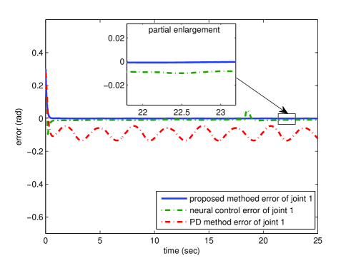
Figure 1: Tracking error of joint 1.

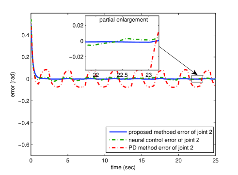
Figure 2: Tracking error of joint 2.

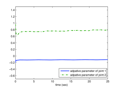
Figure 3: Adaptive law $\hat{W}_{i}(i=1,2)$.

Figure 4: Controller output $v_{1}$.

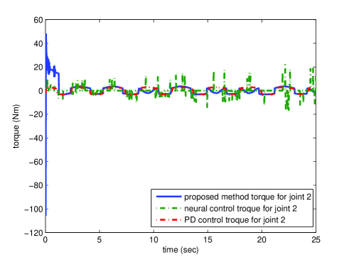
Figure 5: Controller output $v_{2}$.

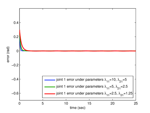
Figure 6: Tracking error of joint 1 under different controller parameters.

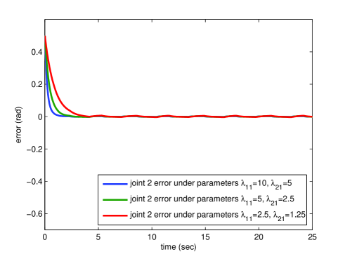
Figure 7: Tracking error of joint 2 under different controller parameters.

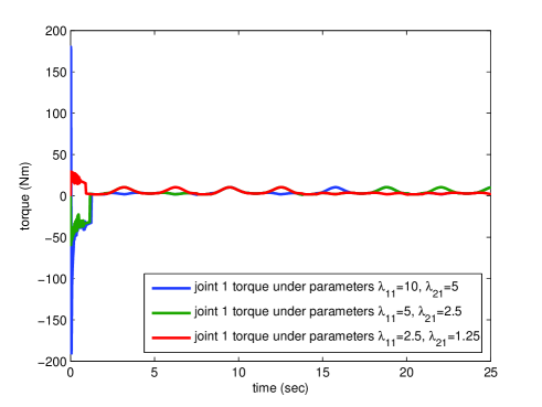
Figure 8: Controller output $v_{1}$ under different controller parameters.

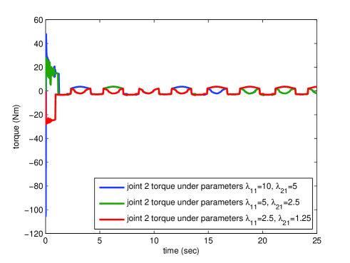
Figure 9: Controller output $v_{2}$ under different controller parameters.

References

• Ge, Ren, Tee, and Lee (2009) S. S. Ge, B. Ren, K. P. Tee, and T. H. Lee, “Approximation-based control of uncertain helicopter dynamics,” IET Control Theory and Applications, vol. 3, no. 7, pp. 941-956, 2009.
• Ge, Li, Yang (2011) S. S. Ge, Z. Li and H. Yang, “Data driven adaptive predictive control for holonomic constrained under-actuated biped robots,” IEEE Transactions on Control Systems Technology, vol. 20 , no. 3, pp. 787-795, 2012.
• Cui, Ge, How, Choo (2010) R. Cui, S. S. Ge, B. V. E. How, Y. S. Choo, “Leader-follower formation control of underactuated autonomous underwater vehicles,” Ocean Engineering, vol. 37, no. 17, pp. 1491-1502, 2010.
• Hua, Wang, Guan (2008) C. C. Hua, Q. G. Wang, X. P. Guan, “Adaptive Tracking Controller Design of Nonlinear Systems With Time Delays and Unknown Dead-Zone Input,” IEEE Trans. Autom. Control, vol. 53, no. 7, pp. 1753-1759, 2008.
• Chen, Liu, Lin (2013) B. Chen, X. Liu, K. Liu and C. Lin, “Fuzzy aproximation-based adaptive control of nonlinear delayed systems with unknown dead zone,” IEEE Trans. Fuzzy System, available on line.
• Zhou (2008) J. Zhou, “ Decentralized adaptive control for large-scale time-delay systems with dead-zone input,” Automatica, vol. 44, no. 3, pp. 1790-1799, 2008.
• Ge, Hang, Zhang (1999) S. S. Ge, C. C. Hang, T. Zhang, “A direct adaptive controller for dynamic systems with a class of nonlinear parameterizations,” Automatica, vol. 35, pp. 741-747, 1999.
• Zhang, Ge (2008) T. P. Zhang and S. S. Ge, “Adaptive dynamic surface control of nonlinear systems with unknown dead zone in pure feedback form,” Automatica, vol. 44, no. 7, pp. 1895-1903, 2008.
• Zhang, Ge (2007) T. P. Zhang and S. S. Ge, “Adaptive neural control of MIMO nonlinear state time-varying delay systems with unknown dead-zones and gain signs,” Automatica, vol. 43, no. 6, pp. 1021-1033, 2007.
• Ge, Hong, Lee (2005) S. S. Ge, F. Hong, and T. H. Lee, “ Robust adaptive control of nonlinear systems with unknown time delays,” Automatica, vol. 41, no. 7, pp. 1181-1190, 2005.
• Shyu, Liu, Hsu (2005) K. K. Shyu, W. J. Liu, K. C. Hsu, “Design of large-scale time-delayed systems with dead-zone input via variable structure control,” Automatica, vol. 41, no. 7, pp. 1239-1246, 2005.
• Ge, Li (2014) S. S. Ge, and Z. J. Li, “Robust Adaptive Control for a Class of MIMO Nonlinear Systems by State and Output Feedback,” IEEE Transactions on Automatic Control, vol. 59, no. 6, pp. 1624-1629, June 2014.
• Slotine, Li (1993) J.-J. E. Slotine and W. Li, Applied nonlinear control, Upper Saddle River, NJ: Prentice-Hall, 1991.
• Ge, Lee, Harris (1998) S. S. Ge, T. H. Lee, and C. J. Harris, Adaptive neural network control of robot manipulators, World Scientific, London, 1998.
• Li, Ge, Wang (2008) Z. Li, S. S. Ge, Z. Wang, “Robust adaptive control of coordinated multiple mobile manipulators,” Mechatronics, vol. 18, pp. 239-250, 2008.
• Li, Ding, Gao, Duan, Su (2013) Z. Li, L. Ding, H. Gao, G. Duan, C.-Y. Su, “Trilateral tele-operation of adaptive fuzzy Force/motion control for nonlinear teleoperators with communication random delays,” IEEE Transactions on Fuzzy Systems, vol. 21, no. 4, pp. 610-623, August 2013.
• Xu, Ioannou (2003) H. Xu and P. A. Ioannou, “Robust Adaptive Control for a Class of MIMO Nonlinear Systems With Guaranteed Error Bounds,” IEEE Transactions on Automatic Control, vol. 48, no. 5, pp. 928-742, 2003.
• Gentle (2007) J. E. Gentle, Matrix Algebra: Theory, Computations, and Applications in Statistics, Springer, 2007.