Conserved Spin Quantity in Strained Hole Systems with Rashba and Dresselhaus Spin-Orbit Coupling

Abstract

We derive an effective Hamiltonian for a (001)-confined quasi-two-dimensional hole gas in a strained zincblende semiconductor heterostructure including both Rashba and Dresselhaus spin-orbit coupling. In the presence of uniaxial strain along the $\left\langle 110\right\rangle$ axes, we find a conserved spin quantity in the vicinity of the Fermi contours in the lowest valence subband. In contrast to previous works, this quantity meets realistic requirements for the Luttinger parameters. For more restrictive conditions, we even find a conserved spin quantity for vanishing strain, restricted to the vicinity of the Fermi surface.

I Introduction

One of the most critical challenges for spintronic devices, as the often mentioned spin-field-effect-transistor due to Datta and DasDatta and Das (1990), lies in the control of the carrier spin lifetime. The latter is limited by the spin relaxation and dephasing processes in semiconductors. The predominant mechanism of the spin relaxation in such devices is of Dyakonov-Perel typeD’yakonov and Perel’ (1971). To extend the application of spintronic devices to the non-ballistic/diffusive regime with spin-independent scattering, it is of particular interest to find conditions for the electrons/holes in the semiconductors which result in symmetries that correspond, according to Noether’s theoremNoether (1918), to the conservation of spin. These symmetries enable to detect long-lived or even persistent spin states, i.e., states which do not relax in time. In structurally confined two-dimensional electron gases (2DEG) such persistent solutions have been predicted for a special interplay between the linear-in-momentum DresselhausDresselhaus (1955) and Bychkov-RashbaRashba (1960); J. Ohkawa and Uemura (1974) spin-orbit coupling (SOC) by J. Schliemann et al., Ref. Schliemann et al., 2003, and were extended by B.A. Bernevig et al., Ref. Bernevig et al., 2006. These special states have been later confirmed by means of optical experimentsKoralek et al. (2009); Walser et al. (2012). The first type of SOC appears in semiconductors with broken inversion symmetry in the crystal structure (bulk inversion asymmetry (BIA)), the second one occurs when a structure inversion asymmetry (SIA) in consequence of an asymmetric confining potential in the semiconductor heterostructure is present.

In contrast to electron systems, the SOC is distinct and much more complex for holes although the underlying fundamental mechanism, described by the Dirac equation, is the same. Since the conduction band, for most semiconductors, is an s-type energy band and the valence band is of p-type, the qualitative variation comes from the different total angular momentum, which is $j=3/2$ in the valence band, giving rise to heavy and light holes (HH, LH) and the split-off holes. As the mixing of HH and LH strongly influences the SOC, the reduction of dimensionality, like the 2D hole gases (2DHG) in semiconductor heterostructures, has an immediate effect.Rashba and Sherman (1988) This is due to the fact that the size quantization causes an energy separation between HH and LH states even at a vanishing in-plane Bloch wave vector which affects the strength of the HH-LH mixing and thus the SOC at finite $k$ vectors. As a consequence, the magnitude of the SOC, especially the prefactor for Rashba SOC, depends sensitively on the confinement, as will be discussed in this paper. Conversely, the Rashba SOC in the lowest conduction band is hardly affected by the size quantization. This is due to the s-type character of the energy band and also since the SOC is mainly determined by the energy gaps between the bulk bands. These energy gaps, however, do not differ significantly if adding a confinement. For a proper description of the hole system, compared to electron systems, a substantially higher number of SOC terms is needed and requires approximations for an analytical investigation at an early stage.

Also, internal or external strain can yield significant consequences to the hole band structure. The reason is that it introduces additional couplings between the HH and LH bands, whereas - assuming a semiconductor with a direct bandgap - the conduction band is only indirectly affected due to the interaction with the strain-altered valence band.Sun et al. (2010, 2007); Seiler et al. (1977); Cardona et al. (1988) Moreover, the cubic crystal structure of the semiconductor has an imprint on the symmetry of the hole spectrum as can be seen in the warping of the Fermi contours and these always follow the strained crystal symmetry.

Nonetheless, despite their complexity hole systems offer opportunities not available in electron systems and are particularly interesting for practical device applications for several reasons. First, the large effective mass $m^{*}$ of holes compared to conduction band electrons diminishes the kinetic term such that contributions from SOC become more important. Second, the p-wave character of the HH and LH states reduces the hyperfine interaction of the carrier spin with the nuclei. This allows in principle for long spin relaxation/dephasing times.Korn et al. (2010); Kugler et al. (2009) Another important aspect is the strength of the SOC in hole systems which can reach several meV in the splitting as, e.g., shown in GaAs/AlGaAs heterostructuresHirmer et al. (2011); Grbić et al. (2008). All these features of p-type systems facilitate a very effective manipulation of carrier spins and, hence, motivate further studies of hole gases in semiconductors as the one presented here. Moreover, since in a 2DEG the conserved spin quantities are always limited by a $k$-cubic Dresselhaus contribution the question arises whether this is also the case for the 2D hole systems.

An appealing continuation of the findings on spin-preserving symmetries in electron systems is the analysis of persistent spin states in hole systems as done recently in Refs. Sacksteder and Bernevig, 2014; Dollinger et al., 2014. However, these publications presuppose materials with strongly restricted and unusual band structures. Following Ref. Dollinger et al., 2014, a strainless sample with both Rashba and Dresselhaus SOC allows for the existence of a persistent spin helix (PSH) in a 2DHG only in the case of a vanishing Luttinger parameter $\gamma_{3}$ with $\gamma_{1}>0$ and $\gamma_{2}>0$.Dollinger et al. (2014) Most of the semiconductors can only be properly described using a band model where $\gamma_{2}<\gamma_{3}$Vurgaftman et al. (2001); Yu and Cardona (2010); Winkler (2003)(App. A), though. In Ref. Sacksteder and Bernevig, 2014 the PSH was found in the presence of finite strain and Rashba SOC where the condition for the Luttinger parameters is restricted by a different, however, also unusual condition $\gamma_{2}=-\gamma_{3}$.

Another approximation which is often applied is to drop all invariants in the bulk Hamiltonian which lead to BIA and have relatively small expansion coefficients. This procedure is justified in bulk systems. In 2DHGs, this approach leads to a model Hamiltonian with both Rashba and Dresselhaus SOC being essentially cubic in momentumBulaev and Loss (2005); Dollinger et al. (2014), in contrast to 2DEGs where the dominant Rashba term is linear and the Dresselhaus term linear and cubic in momentum.Winkler (2003) However, recent publicationsLuo et al. (2010); Durnev et al. (2014) which are related to the seminal paper by Rashba and Sherman, Ref. Rashba and Sherman, 1988, show that the relevance of the linear Dresselhaus terms in 2DHG has been underestimated: the abovementioned estimations are thus questionable and fail at least for the standard compound GaAs.

In this paper, we present conditions for a wider range of semiconductors including strain, linear and cubic Dresselhaus and Rashba SOC under which conserved spin quantities can be found.
This paper is organized as follows. In the next section, we derive an effective two-dimensional heavy/light hole like Hamiltonian including strain, Dresselhaus and Rashba SOC. In Sec. III, we derive the conditions for the existence of a conserved spin quantity. Thereby we discuss its realizability and apply our findings to a prominent compound, InSb. Finally, we summarize our results.

II The Model

The aim of our investigation is to identify the appropriate interplay between BIA (Dresselhaus SOC), a confining potential $V({\bf r})$ (build-in and/or external) causing SIA, and strain (either externally imposed using, e.g., the piezoelectric effect or induced by the epitaxial growth process) which gives rise to a conserved spin quantity in the hole system. To find analytic conditions we derive an effective HH/LH like $2\times 2$ model, depending on the character of the up-most valence band. Starting point is a $4\times 4$ model which is derived form the extended Kane model and includes the Luttinger HamiltonianLuttinger (1956).

II.1 Effective $4\times 4$ Hole Hamiltonian

Hereafter, we choose the coordinates to be $\hat{x}\parallel[100]$, $\hat{y}\parallel[010]$ and $\hat{z}\parallel[001]$. We use the Luttinger parameters $\gamma_{i}$, the bare electron mass $m_{0}$ and elementary charge $e>0$, the electric field $\mathcal{E}_{z}$, the total angular momentum $\mathbf{J}$ for $j=3/2$ and the symmetrized anticommutator $\left\{A,B\right\}=\left(AB+BA\right)/2$.

The applied model which we use as a starting point for the investigation is an effective $4\times 4$ Hamiltonian given by

$$\mathcal{H}={} \mathcal{H}_{\text{L}}+\mathcal{H}_{\text{BIA}}+\mathcal{H}_{\text{S}}+V.$$ (1)

The first term represents the Luttinger Hamiltonian for III-V semiconductors

$$\mathcal{H}_{\text{L}}={} -\frac{\hbar^{2}}{2m_{0}}\Bigg{(}\gamma_{1}\mathbf{k}^{2}-2\gamma_{2}\left[\left(J_{x}^{2}-\frac{1}{3}\mathbf{J}^{2}\right)k_{x}^{2}+\text{c.p.}\right]$$

$$-4\gamma_{3}\left[\{J_{x},J_{y}\}\{k_{x},k_{y}\}+\text{c.p.}\right]\Bigg{)},$$ (2)

where c.p. denotes the cyclic permutation of the preceding indices. The second term $\mathcal{H}_{\text{BIA}}$ accounts for the Dresselhaus SOC and is decomposed by the theory of invariants asWinkler (2003)

$$\mathcal{H}_{\text{BIA}}={} \frac{2}{\sqrt{3}}\,C_{k}\left(k_{x}\{J_{x},J_{y}^{2}-J_{z}^{2}\}+\text{c.p.}\right)$$

$$+b_{41}^{8v8v}\left(\{k_{x},k_{y}^{2}-k_{z}^{2}\}J_{x}+\text{c.p.}\right)$$

$$+b_{42}^{8v8v}(\{k_{x},k_{y}^{2}-k_{z}^{2}\}J_{x}^{3}+\text{c.p.})$$

$$+b_{51}^{8v8v}(\{k_{x},k_{y}^{2}+k_{z}^{2}\}\{J_{x},J_{y}^{2}-J_{z}^{2}\}+\text{c.p.})$$

$$+b_{52}^{8v8v}(k_{x}^{3}\{J_{x},J_{y}^{2}-J_{z}^{2}\}+\text{c.p.}).$$ (3)

It includes a $k$-linear term proportional $C_{k}$ which is usually rather smallCardona et al. (1988); Winkler (2003) and thus often not consideredDurnev et al. (2014); Bulaev and Loss (2005); Dollinger et al. (2014); Rashba and Sherman (1988). An exemplary comparison of the remaining cubic contributions with the extended Kane model in App. B.2 shows that in a bulk system the term proportional to $b_{41}^{8v8v}$ is the most relevant one. However, in 2D size quantization leads to additional linear terms that may become significant in certain parameter regimesDurnev et al. (2014); Rashba and Sherman (1988); Luo et al. (2010). We note that there are discrepancies in the perturbative determination of the coefficients $b_{i}^{8v8v}$ as outlined in App. B.2.

Furthermore, the effect of strain is described by the Bir-Pikus strain Hamiltonian $\mathcal{H}_{\text{S}}$Bir and Pikus (1974); Sacksteder and Bernevig (2014):

$$\mathcal{H}_{\text{S}}={} \sum_{i}\left(a\,\epsilon_{ii}+b\;\epsilon_{ii}\,J_{i}^{2}+d\,\sum_{j,\;j\neq i}\epsilon_{ij}\,\{J_{i},J_{j}\}\right).$$ (4)

We assume the strain, with $\epsilon_{ij}$ being the symmetric strain tensor, to be uniaxial in-plane or biaxial in-plane. As a consequence, an in-plane strain with the tensor components $\epsilon_{xx}$, $\epsilon_{yy}$, $\epsilon_{xy}$ yields only one extra strain component, $\epsilon_{zz}$. Thus, we set $\epsilon_{xz}=\epsilon_{yz}=0$ in Eq. (4). One should stress that slightly different notations occur in the literature for the deformation potentials $a$, $b$ and $d$. Some relations between different definitions are listed in App. D.1. Here, we follow Ref. Sacksteder and Bernevig, 2014. Thus, the potentials $b$ and $d$ are positive whereas $a$ can be positive or negative.

Eventually, the potential $V=V_{\text{E}}+V_{\text{c}}$ includes the confining potential $V_{\text{c}}(z)$ and the external potential $V_{\text{E}}(z)$. The latter causes structure inversion asymmetry (SIA) which induces Rashba SOC. We assume the potential $V$ to depend only on the $z$-coordinate, which is pointing in the growth direction $[001]$ of the semiconductor heterostructure. More explicitly,

$$V_{\text{E}}(z)= \mathbbm{1}_{4\times 4}\cdot e\,\mathcal{E}_{z}z,$$ (5)

and an infinite square well of width $L$ with

$$V_{\text{c}}(z)=\mathbbm{1}_{4\times 4}\cdot\begin{cases}0&\text{for}\;z\in\left[0,L\right],\\ \infty&\text{otherwise}.\end{cases}$$ (6)

Notice that the discontinuity of the potential $V_{\text{c}}$ can result in non-hermitian matrix elements of $k_{z}^{3}$ if not taken care. This problem can be resolved by a regularization procedure as shown in Ref. PhysRevB.90.195410. Furthermore, contributions due to boundary effects which result from the presence of heterointerfaces are assumed to be small. Such an interface can allow for additional HH-LH mixing.Ivchenko and Pikus (1995); Ivchenko et al. (1996); Magri and Zunger (2000); Luo et al. (2010) A possible alternation of spin relaxation due to interface effects will be discussed elsewhere.

II.2 Effective $2\times 2$ Model for the First Subband

In the following, we choose the basis states in such a way that the upper left block represents the HH the lower right block the LH subspace:

$$\mathcal{H}=\begin{pmatrix}\mathcal{H}_{\text{HH}}&\mathcal{H}_{\text{HH-LH}}\\ \mathcal{H}_{\text{LH-HH}}&\mathcal{H}_{\text{LH}}\end{pmatrix}.$$ (7)

The confinement in $z$-direction allows for a further simplification of the model to an effective $2\times 2$ Hamiltonian using quasi-degenerate perturbation theory (Löwdin’s partitioning). The full Hamiltonian $\mathcal{H}$ is separated into two parts

$$\mathcal{H}=\mathcal{H}_{0}+\mathcal{H}^{\prime},$$ (8)

according to App. B.1. The partition is, in general, not uniquely defined and different ways of splitting $\mathcal{H}$ are possible. For the given system, a meaningful decomposition is the one which allows a projection on the subspace of a particular HH or LH like subband. Here, we select $\mathcal{H}_{0}$ to contain the diagonal elements of $\mathcal{H}_{\text{L}}+\mathcal{H}_{\text{S}}+V_{\text{c}}(z)$ at $k_{x}=k_{y}=0$, and $\mathcal{H}^{\prime}$ is treated as a perturbation with respect to the appropriate inverse splitting $1/\Delta_{\text{hl}}$, ($1/\Delta_{\text{hh}}$) between a HH like and a LH(HH) like subband. The energy splitting $\Delta_{\text{hl}}$ is due to both the spatial confinement in the [001] direction and the imposed strain.

According to the confinement, the eigenstates of $\mathcal{H}_{0}$ are given by $\ket{j,m_{j}}\ket{n}$, the product of the eigenstates of the total angular momentum $\mathbf{J}$ with $j=3/2,m_{j}=\pm 1/2$ for LH and $m_{j}=\pm 3/2$ for HH and the subband index of $z$-quantization $n\in\mathbbm{N}^{*}$. The eigenfunctions of the quantum well in position space are given by $\braket{z}{n}=\sqrt{2/L}\sin(z\,n\,\pi/L)$ which lead to the matrix elements of the $k_{i}$ and $z$ operators given by

$$\braket{n}{k_{z}}{l}={} \frac{2inl\left((-1)^{l+n}-1\right)}{L\left(n^{2}-l^{2}\right)}(1-\delta_{nl}),$$ (9)

$$\braket{n}{k_{z}^{2}}{l}={} \left(\frac{\pi n}{L}\right)^{2}\delta_{nl},$$ (10)

$$\braket{n}{z}{l}={} \begin{cases}\frac{L}{2}&\text{for }n=l,\\ \frac{4nlL\left((-1)^{l+n}-1\right)}{\pi^{2}\left(l^{2}-n^{2}\right)^{2}}&\text{otherwise.}\end{cases}$$ (11)

The eigenenergies of $\mathcal{H}_{0}$ (twofold degenerate) according to the sub-spaces are given by

$$E_{\text{HH}}(n)={} -\frac{\hbar^{2}}{2m_{0}}(\gamma_{1}-2\gamma_{2})\braket{k_{z}^{2}}n^{2},$$ (12)

$$E_{\text{LH}}(n)={} -\frac{\hbar^{2}}{2m_{0}}(\gamma_{1}+2\gamma_{2})\braket{k_{z}^{2}}n^{2}+\delta,$$ (13)

where $\delta=b\left(\epsilon_{xx}+\epsilon_{yy}-2\epsilon_{zz}\right)$ corresponds to the diagonal shear strain tensor and $\braket{k_{z}^{2}}\equiv\braket{1}{k_{z}^{2}}{1}$. For simplification we subtracted an overall constant energy shift of $\Delta E=-\sum_{i}(a+3b/4)\epsilon_{ii}-(3/2)b\epsilon_{zz}$. It becomes apparent that strain effects as well as the confining potential lift the degeneracy of HH and LH bands at $k_{\parallel}\equiv\sqrt{k_{x}^{2}+k_{y}^{2}}=0$.

In the following, the in-plane strain contribution will be rewritten, according to Ref. Sacksteder and Bernevig, 2014, defining an in-plane strain amplitude $\beta$ and orientation $\theta$ as

$$\beta^{2}e^{2i\theta}:={} \frac{m_{0}}{\hbar^{2}\gamma_{3}}(b\left(\epsilon_{xx}-\epsilon_{yy}\right)+2id\epsilon_{xy}).$$ (14)

The effective Hamiltonian for the lowest subband is now derived by quasi-degenerate perturbation theory (see App. B.1). Thereby, the lowest subband can be either a HH like or a LH like subband, depending on the magnitude and type of strain. Up to third order in the energy splitting it yields

$$\mathcal{H}_{\text{eff}}\approx{} \sum_{p=0}^{3}\mathcal{H}^{(p)}$$ (15)

$$={} \sum_{p=0}^{3}\left(E_{\text{kin}}^{(p)}+V_{\text{eff}}^{(p)}\right)\cdot\mathbbm{1}_{2\times 2}+\bm{\Omega}^{(p)}\cdot\bm{\sigma}$$ (16)

with the Pauli matrices $\sigma_{i}$ and the $\mathcal{H}^{(p)}$, where the superscript $(p)$ indicates the order in the perturbation (App. B.1). Additionally, we will neglect terms of the order of $\mathcal{O}(k^{4})$.

We would like to mention some properties of the perturbation theory first. Concerning the decomposition of the Hamiltonian, it should be stressed that if we instead choose $\mathcal{H}_{0}=\mathcal{H}_{\text{L}}+\mathcal{H}_{\text{S}}$, that is, without the confinement potential, we can make use of the non-commutativity of the momentum operator $k_{z}$ and the position operator $z$ to derive a finite Rashba coefficient as done in Refs. Winkler, 2003; Sacksteder and Bernevig, 2014. However in this case, the energy splitting $\Delta_{\text{hl}}$ cannot be a result of the subband quantization, but only have strain as an origin. This approximation may be justified if the strain splitting is much larger than the subband splitting. Yet, since we consider a quasi 2D system, the subband splitting is an essential effect and we are thus to choose the partitioning as described above.

An important observation of the perturbation presented in this paper is that a finite Rashba spin-orbit (SO) field, resulting from the coupling between different subbands, can only be obtained by third or higher order perturbation theory. This is due to the fact that the diagonal elements of $\mathcal{H}^{\prime}$, Eq. (8), and thus $\mathcal{E}_{z}$, are not yet involved in the second order, according to Eq. (67). In addition, it will be shown in the following that given a HH(LH) like ground state it is necessary to include, in addition to the first LH(HH) like subband, also the second HH(LH) like subband in the perturbation procedure to yield a finite contribution due to Rashba SOC.

Concerning the significance of the various Dresselhaus contributions in Eq. (3) we mentioned earlier, Sec. II.1, that in the bulk system keeping only the cubic term proportional $b_{41}^{8v8v}$ is a good approximation. This is due to its large value compared to the other cubic terms.Winkler (2003) However, the size quantization causes an additional linear Dresselhaus contribution for HHs that would not appear if only the term proportional $b_{41}^{8v8v}$ was considered. For the light holes, the situation is different as the term proportional $b_{41}^{8v8v}$ already yields a linear term which clearly dominates over the remaining linear contributions. As a result, we will take into account the effect of the $k$-linear terms generated in the first order perturbation by the terms proportional $C_{k}$, $b_{42}^{8v8v}$ and $b_{51}^{8v8v}$ only in case of a HH like ground state and neglect them in case of a LH like ground state. The coefficient $b_{52}^{8v8v}$ yields only a small cubic term which can be disregarded. Based on its large value, for higher order BIA corrections we incorporate solely terms proportional to $b_{41}^{8v8v}$.

Depending on the nature of the strain, the splitting can lead to either a lowest HH like or LH like subband. If we, e.g., specify to the case of uniaxial compressive stress in [110] direction, we obtain $\delta<0$ since $\epsilon_{xx}=\epsilon_{yy}<0$ and $\epsilon_{zz}>0.$Sun et al. (2007) Therefore, the splitting between HH and LH is enhanced and the topmost subband is HH for arbitrary material since $\gamma_{i}>0$. Consequently, we have to distinguish two cases:

II.2.1 System with a Heavy-Hole Like Ground State

Assuming the ground state being HH like and applying third order Löwdin perturbation theory, we get for the part of the Hamiltonian which is proportional to unity in spin space, according to Eq. (16),

$$E_{\text{kin,HH}}={} E_{\text{kin,+}},$$ (17)

$$V_{\text{eff,HH}}={} V_{\text{eff},+}(\Delta_{\text{h1,h2}}),$$ (18)

where we defined

$$E_{\text{kin},\pm}=-\frac{\hbar^{2}}{2m_{0}}\left(\gamma_{1}\pm\gamma_{2}\right)k_{\parallel}^{2}\pm\frac{1}{\Delta_{\text{h1,l1}}}\left\{\frac{3}{4}\left(b_{41}^{8v8v}\braket{k_{z}^{2}}\right)^{2}k_{\parallel}^{2}+\frac{3\hbar^{4}}{2m_{0}^{2}}\beta^{2}\gamma_{3}^{2}\left[\frac{\gamma_{2}}{\gamma_{3}}\left(k_{x}^{2}-k_{y}^{2}\right)\cos(2\theta)+2k_{x}k_{y}\sin(2\theta)\right]\right\}$$ (19)

and

$$V_{\text{eff},\pm}(\Delta)=\sum_{i}\left(a+\frac{3}{4}b\right)\epsilon_{ii}+\frac{3}{2}b\epsilon_{zz}-\frac{\hbar^{2}\braket{k_{z}^{2}}}{2m_{0}}\left(\gamma_{1}\mp 2\gamma_{2}\right)+\frac{e\mathcal{E}_{z}L}{2}\pm\frac{3\hbar^{4}}{4m_{0}^{2}\Delta_{\text{h1,l1}}}\beta^{4}\gamma_{3}^{2}+\frac{256L^{2}e^{2}\mathcal{E}_{z}^{2}}{81\Delta}.$$ (20)

The energy gaps are given by $\Delta_{\text{ln,hm}}=E_{\text{LH}}(n)-E_{\text{HH}}(m)$ and $\Delta_{\text{hn,lm}}$ analogously. The effective vector field $\bm{\Omega}$ due to Rashba and Dresselhaus SOC, which is modified by the presence of strain, yields

$$\bm{\Omega}_{\text{HH}}=\bm{\Omega}_{+}$$ (21)

with components given by

$$\Omega_{x,\pm}={} \lambda_{\text{D},\pm}\Bigg{\{}k_{x}k_{y}^{2}\left(\gamma_{2}\mp 2\gamma_{3}\right)-k_{x}^{3}\gamma_{2}+\beta^{2}\gamma_{3}\left[\pm k_{y}\left(\frac{k_{x}^{2}}{\braket{k_{z}^{2}}}-1\right)\sin(2\theta)+k_{x}\left(\frac{k_{y}^{2}}{\braket{k_{z}^{2}}}-1\right)\cos(2\theta)\right]\Bigg{\}}$$

$$+\eta_{\pm}k_{x}+\lambda_{\text{R},\pm}\left[\pm\left(\gamma_{2}\pm 2\gamma_{3}\right)k_{x}^{2}k_{y}\mp\gamma_{2}k_{y}^{3}+\beta^{2}\gamma_{3}\left(\pm k_{y}\cos(2\theta)+k_{x}\sin(2\theta)\right)\right],$$ (22a)

$$\Omega_{y,\pm}={} \lambda_{\text{D},\pm}\Bigg{\{}\pm k_{x}^{2}k_{y}\left(\gamma_{2}\mp 2\gamma_{3}\right)\mp k_{y}^{3}\gamma_{2}+\beta^{2}\gamma_{3}\left[k_{x}\left(\frac{k_{y}^{2}}{\braket{k_{z}^{2}}}-1\right)\sin(2\theta)\mp k_{y}\left(\frac{k_{x}^{2}}{\braket{k_{z}^{2}}}-1\right)\cos(2\theta)\right]\Bigg{\}}$$

$$\pm\eta_{\pm}k_{y}\pm\lambda_{\text{R},\pm}\left[\pm\left(\gamma_{2}\pm 2\gamma_{3}\right)k_{x}k_{y}^{2}\mp\gamma_{2}k_{x}^{3}+\beta^{2}\gamma_{3}\left(k_{y}\sin(2\theta)\mp k_{x}\cos(2\theta)\right)\right],$$ (22b)

$$\Omega_{z,\pm}={} 0.$$ (22c)

Here, the Dresselhaus coefficients $\eta_{\pm}$, $\lambda_{\text{D},\pm}$ and the Rashba coefficient $\lambda_{\text{R},\pm}$ are given by

$$\eta_{+}={} -\frac{\sqrt{3}}{2}C_{k}-\frac{3}{4}\left(b_{\text{42}}^{8v8v}+b_{\text{51}}^{8v8v}\right)\braket{k_{z}^{2}}$$ (23)

$$\eta_{-}={} -b_{\text{41}}^{8v8v}\braket{k_{z}^{2}}$$ (24)

$$\lambda_{\text{D},\pm}={} \pm\frac{3\hbar^{2}}{2m_{0}\Delta_{\text{h1,l1}}}b_{\text{41}}^{8v8v}\braket{k_{z}^{2}},$$ (25)

$$\lambda_{\text{R},+}={} \frac{128\hbar^{4}e\mathcal{E}_{z}\gamma_{3}}{9\pi^{2}m_{0}^{2}\Delta_{\text{h1,l1}}\Delta_{\text{h1,h2}}},$$ (26)

$$\lambda_{\text{R},-}={} \frac{128\hbar^{4}e\mathcal{E}_{z}\gamma_{3}}{9\pi^{2}m_{0}^{2}\Delta_{\text{l1,h1}}\Delta_{\text{l1,l2}}}.$$ (27)

The index $(\pm)$ distinguishes the case of a system with a HH like ground state $(+)$ from the one with a LH like ground state $(-)$.

Notice that given a vanishing $\gamma_{3}$ the dominant contribution due to Rashba SOC vanishes, too. Only a contribution as a result of the coupling to conduction bands is left, which is of higher than third order: In the bulk system, for most semiconductors, the dominant invariant in the extended Kane modelKane (1957), which is present due to SIA, is given byWinkler (2003)

$$\mathcal{H}_{8v8v}^{r}=r_{41}^{8v8v}((k_{y}\mathcal{E}_{z}-k_{z}\mathcal{E}_{y})J_{x}+\text{c.p.}).$$ (28)

If the bulk system is reduced to an effective two-dimensional system, the according counterpart of this term in an effective $2\times 2$ Hamiltonian can be calculated using Löwdin perturbation theory as done above, keeping the factor $r_{41}^{8v8v}$ unchanged. However, as mentioned in Ref. Dollinger et al., 2014, for a HH like ground state this resulting term is of higher order than the one given proportional to $\lambda_{\text{R}}$ (although represented by the same invariants). This can be understood by recalling the root of the coefficient $r_{41}^{8v8v}$: It is the coupling between valence and conduction bands. In contrast, if a confinement is present, the contribution resulting from Rashba SOC in the effective HH system is dominated by the splitting between HH and LH like subbands. In the case of a LH like ground state an additional $k$-linear Rashba term proportional to $r_{41}^{8v8v}$ appears already in third order perturbation theory. The angular momentum matrix $J_{x}$ is zero in the HH subspace but has finite matrix elements in the LH subspace. Since the prefactor $r_{41}^{8v8v}$ contains terms which are inversely proportional to the band gapWinkler (2003), this contribution can be neglected since we assume the conduction bandgap to be much larger than the subband splitting. The contribution stemming from BIA has a different nature: The parameter $b_{41}^{8v8v}$, which is connected with the invariant $(\{k_{x},k_{y}^{2}-k_{z}^{2}\}J_{x}+\text{c.p.})$ in the Kane model, is mainly defined through the valence band $\Gamma_{8v}$ and conduction band $\Gamma_{6c}$ gap $E_{0}$. Thus, it is hardly affected by the subband quantization. Moreover, in contrast to the Rashba contribution, the corresponding Dresselhaus term in the confined system appears already in second order of the applied perturbation. Hence, we also neglect higher order contributions due to BIA.

II.2.2 System with a Light-Hole Like Ground State

According to Eqs. (12) and (13), on condition that $\delta>2\hbar^{2}\pi^{2}\gamma_{2}/(m_{0}L^{2})$ the ground state of the valence band is the first LH like subband. As in the case of a HH like ground state, we do not obtain a $z$-component in the effective SO field. However, in first order Löwdin perturbation theory, Eq. (65), we obtain an additional linear term $\eta_{-}$ and a cubic term $\bm{\Omega}_{b}$ proportional to $b_{41}^{8v8v}$. Furthermore, terms appear in third order which couple the electric field $\mathcal{E}_{z}$ with the Dresselhaus term proportional to $b_{41}^{8v8v}$, App. B.3. Since the SOC is a small correction, these terms are much smaller than the one not mixing both factors. Thus, according to the previous case of a HH like ground state, we have

$$E_{\text{kin,LH}}={} E_{\text{kin},-},$$ (29)

$$V_{\text{eff,LH}}={} V_{\text{eff},-}(\Delta_{\text{l1,l2}})+\delta.$$ (30)

The effective vector field $\bm{\Omega}$ due to Rashba and Dresselhaus SOC yields

$$\bm{\Omega}_{\text{LH}}=\bm{\Omega}_{-}+\bm{\Omega}_{b}$$ (31)

with the additional term

$$\bm{\Omega}_{b}=b_{41}^{8v8v}\left\{k_{x}k_{y}^{2},-k_{x}^{2}k_{y},0\right\}^{\top}.$$ (32)

II.3 Summarized Results

In summary, by developing an effective $2\times 2$ model for a 2DHG we worked out the dominant contributions due to strain ($\beta$, $\theta$), Rashba ($\lambda_{R}$) and Dresselhaus SOC ($\eta$, $\lambda_{D}$) to be considered in Eq. (16). The interplay between strain and Rashba or Dresselhaus SOC yields additional terms that are linear respectively linear as well as cubic in momentum. Thereby, we find that in contrast to the Rashba contribution the according Dresselhaus term in the confined system appears already in second order Löwdin perturbation theory. In respect of finding a conserved spin quantity we extracted the effective vector fields $\bm{\Omega}_{\text{HH}}$ for a HH like ground state and $\bm{\Omega}_{\text{LH}}$ for a LH like ground state in Eqs. (21) and (31). The fields cover a wide parameter space. In the next section, this will allow for identifying conserved spin quantities which do not require parameter-configurations which are difficult to realize in real materials (e.g., $\gamma_{3}=0$ in Ref. Dollinger et al., 2014, $\gamma_{2}=-\gamma_{3}$ in Ref. Sacksteder and Bernevig, 2014). Thus, it facilitates the detection of long-lived spin states in experiments.

III Conserved Spin Quantity

Following the analysis of Ref. Schliemann et al., 2003, our goal is to identify a conserved quantity $\Sigma$ which is directly connected with $k$-independent eigenspinors. The general ansatz is

$$\Sigma=s_{0}\mathbbm{1}_{2\times 2}+\mathbf{s}\cdot\bm{\sigma}.$$ (33)

For this quantity to be conserved, it has to fulfill the relation $\left[\Sigma,\mathcal{H}_{\text{eff}}\right]=0$ which is true for

$$\Omega_{x}s_{z}=\Omega_{y}s_{z}=0\quad\wedge\quad\Omega_{y}s_{x}-\Omega_{x}s_{y}=0.$$ (34)

We are going to prove that one can find two solutions of this problem given by

$$\Sigma_{\xi}=\sum_{{\bf k},k=k_{\parallel F}}\sum_{\alpha\beta}c^{\dagger}_{{\bf k}\alpha}(\sigma_{x}+\xi\sigma_{y})_{\alpha\beta}c_{{\bf k}\beta},$$ (35)

with $\xi=\pm$, if either the strain is absent or its direction fulfills

$$\theta={} \pm\frac{\pi}{4}\equiv\chi\frac{\pi}{4}.$$ (36)

Here, $c^{\dagger}_{{\bf k}\alpha}$ creates a HH(LH) in the spin state $\alpha=\pm$ for $m_{j}=\pm 3/2$ ($m_{j}=\pm 1/2$). We assume that the Fermi wave vector $k_{\parallel F}$ does not deviate much from rotational symmetry and thus can be replaced by its angular average value $k_{\parallel F}\equiv\braket{k_{\parallel F}}_{\varphi}$.Sacksteder and Bernevig (2014); Dollinger et al. (2014) This situation holds for materials close to axial symmetry, i.e., $\gamma_{2}=\gamma_{3}$, and a small strain amplitude $\beta$. Therefore, we transform $\left\{k_{x},k_{y}\right\}^{\top}$ into polar coordinates, $k_{\parallel F}\{\cos(\varphi),\sin(\varphi)\}^{\top}$. Thus, if a hole, with a spin state given by $\{1,\pm\exp(\xi i\pi/4)\}^{\top}/\sqrt{2}$ and $k=k_{\parallel F}$ is injected into the two-dimensional system (including spin-independent scattering processes) its spin is not randomized.

For the in-plane strain, the direction condition basically requires symmetric normal strain components $\epsilon_{xx}=\epsilon_{yy}$ and a non-vanishing shear strain component $\epsilon_{xy}$. This situation can be generated by $\left\langle 110\right\rangle$ uniaxial strain.Sun et al. (2007) We demonstrate this explicitely in App. D.2 for an experimental setup by use of a piezo crystal as done by Habib et al. in Ref. Habib et al., 2007.

As we will see in the following, the constraint on the wave vector ${\bf k}$ of persistent spin states is crucial since it reveals that we found no conserved spin quantity for the whole $k$-space but only for the averaged Fermi contour. However, this constraint is not surprising when we recall the case of persistent spin states in 2DEG. If the SO terms are linear in the wave vector, the condition for the existence of persistent spin states is fulfilled if the Rashba SOC coefficient is equal to the one for the linear Dresselhaus term. In this special case, the SO field is collinear in the whole $k$-space. If the cubic Dresselhaus term is included, we cannot find a quantity $\Sigma$ which commutes with the Hamiltonian $\mathcal{H}$ at every wave vector, though. Nevertheless, if the relations resulting from $[\Sigma,\mathcal{H}]\stackrel{{\scriptstyle!}}{{=}}0$ are Fourier decomposed, similar to the procedure in Ref. Knap et al., 1996, and only the lowest harmonics in the azimuthal angle is considered, one finds a condition for long-lived spin states. In contrast to the case without the cubic contribution, the found symmetry is, however, bound to an appropriate energy.Dollinger (2013) This can also be understood by studying the spin relaxation rates in diffusive n-type wires with Rashba and Dresselhaus SOC. One does not only find an additional spin-relaxation term due to the cubic Dresselhaus but also, the linear Dresselhaus coefficient is shifted.Kettemann (2007) This shift depends on the Fermi energy.

Next, as in the previous section, we consider separately the case of a HH like ground state and the LH like ground state. For the sake of simplicity, we apply the following replacements:

$$\lambda_{\text{D},\pm}={} n_{\text{\tiny HH/LH}}\lambda_{\text{R},\pm},$$ (37)

$$\gamma_{3}={} \Gamma\gamma_{2},$$ (38)

$$\beta={} Bk_{\parallel F},$$ (39)

$$\braket{k_{z}^{2}}={} \left(\frac{k_{\parallel F}}{\kappa}\right)^{2},$$ (40)

and for the HH like state additionally

$$\eta_{+}={} \eta_{0}\gamma_{2}\braket{k_{z}^{2}}\lambda_{\text{D},+}.$$ (41)

In contrast to the discussed effect of the cubic Dresselhaus in an 2DEG, we will find persistent and not only long-lived spin states.

III.1 Conserved Spin Quantity in Case of a HH Like Ground State

Making use of the definitions above and setting $n\equiv n_{\text{\tiny HH}}$ for simplicity, we obtain for $\Sigma_{\xi}$ the following equation according to Eq. (34):

$$0={} \Omega_{y,+}-\xi\Omega_{x,+}$$ (42)

$$={} \left(\cos(\varphi)-\xi\sin(\varphi)\right)$$

$$\cdot\left\{B^{2}\Gamma\xi\left(n+\xi\right)+\chi\left[\xi+n(\eta_{0}/\kappa^{2}-1)\right]\right.$$

$$\phantom{a}+\left[B^{2}\kappa^{2}n\Gamma+2\chi\left(1+\Gamma+n\xi\left(\Gamma-1\right)\right)\right]$$

$$\left.\phantom{aaa}\cdot\cos(\varphi)\sin(\varphi)\right\}.$$ (43)

This equation is fulfilled independently of the polar angle $\varphi$ if the ratio between Dresselhaus and Rashba SOC strength $n$ and the strain strength factor $B$ satisfy the relations

$$n_{\xi,\chi}^{(\pm)}=\xi\frac{2\left(1+\Gamma\right)}{2\left(1-\Gamma\right)-(\xi\chi)\Gamma\kappa^{2}\left(B_{\xi,\chi}^{(\pm)}\right)^{2}}$$ (44)

and

$$B_{\xi,\chi}^{(\pm)}=\sqrt{\frac{\xi\chi\left(4-\kappa^{2}\right)\pm\mathcal{W}}{2\Gamma\kappa^{2}}},$$ (45)

where

$$\mathcal{W}=\sqrt{\kappa^{4}+8\left(1+\Gamma\right)\eta_{0}-8\left(1+2\Gamma\right)\kappa^{2}+16},$$ (46)

and $-B_{\xi,\chi}^{(\pm)}$ are also solutions.

If the $C_{k}$ term in Eq. 23 can be neglected (full expression can be found in App. C) real solutions for $B_{\xi,\chi}^{(\pm)}$ are only found for $\kappa\in A_{\mathrm{sgn}(\xi\cdot\chi)}$ where

$$A_{+}= \left[0,2\sqrt{1+2\Gamma-2\sqrt{\left(1+\Gamma\right)(\Gamma-\eta_{0}/8)}}\right],$$ (47)

$$A_{-}= \left[2\sqrt{1+2\Gamma+2\sqrt{\left(1+\Gamma\right)(\Gamma-\eta_{0}/8)}},\infty\right)$$ (48)

if $\Im(A_{\mathrm{sgn}(\xi\cdot\chi)})=0$ which usually holds as typically $\Gamma>0$ and $\eta_{0}<0$.

In absence of strain, that is, $\beta=0$, the fomulas above yield the following requirements on the ratio $n$ and for the Fermi wave vector $k_{\parallel F}$ to get $\Sigma_{\xi}$:

$$n_{0}{} \equiv n=\xi\frac{1+\Gamma}{1-\Gamma},$$ (49)

$$k_{0}{} \equiv k_{\parallel F}=\sqrt{\frac{\eta_{+}}{2\gamma_{2}\lambda_{\text{D,+}}}\frac{1+\Gamma}{\Gamma}}.$$ (50)

In this scenario, the SO field even vanishes at a specific value $k_{0}$ of the Fermi wave vector in the axially symmetric case, i.e., $\Gamma=1$. For this purpose, both linear and cubic Dresselhaus contributions are crucial. Hence, this solution was not existent in our previous publication Ref. Dollinger et al., 2014. The axially symmetric case demands a vanishing Rashba contribution, $\lambda_{\text{R,+}}/\lambda_{\text{D,+}}\approx 0$. However, for the most semiconductors $\Gamma$ ranges from 1 to 1.5. Thus, the cubic Dresselhaus SOC strength has to outweigh the Rashba SOC strength, i.e., $|\lambda_{\text{D},+}|>|\lambda_{\text{R},+}|$.

More peculiar solutions occur for $\Gamma\neq 1$ or in the presence of strain. For certain parameter configurations, the SO field becomes collinear on the averaged Fermi contour. As a consequence, this SU(2) spin rotation symmetry gives rise to a persistent spin helix.Bernevig et al. (2006) For a start, by setting $\Gamma=-1$, $\chi=\xi=1$ we can recover the solutions presented by Sacksteder et al. in Ref. Sacksteder and Bernevig, 2014. In this case, we obtain $n=0$, which is obvious since Dresselhaus SOC was not considered in Ref. Sacksteder and Bernevig, 2014, and $B=1$, which is consistent with their results. It is remarkable that the presence of the linear Dresselhaus term, which was not considered either by Sacksteder et al., does not alter the result. Note that here, too, the solution for the conserved spin quantity is bound to an averaged Fermi contour by Eq. (39). Moreover, recalling Eq. (34), one finds for these particular parameters a conserved spin quantity for every direction $\theta$, given by

$$\Sigma=\sin(\theta)\sigma_{x}-\cos(\theta)\sigma_{y},$$ (51)

which generalizes the result from the previous publication. Yet, we emphasize that the condition $\Gamma=-1$ is rather unusual for most materials. Regarding the realization of persistent spin states in experiments, it is of interest to analyze whether the constrains allow for realistic (i.e., typical for III-V semiconductors) parameters. Thus, we present a concrete example for the conserved quantities $\Sigma_{\xi}$. At this, we assume $\gamma_{3}-\gamma_{2}>0$, Eq. (60), and $\gamma_{i}>0$ to hold and choose, as an example, $\Gamma=1.2$ for the plots of $n_{\xi,\chi}^{(\pm)}$ and $B_{\xi,\chi}^{(\pm)}$, Fig. 1. In order to draw a general picture and for simplicity we neglected the linear Dresselhaus contribution, i.e., $\eta_{0}\rightarrow 0$. In the range $A_{+}$, i.e., $\xi=\chi$ that comprises realistic values for $\kappa$ (e.g., $\kappa=0.3$ for a confinement width $L=100\,\text{\AA}$ and a small Fermi vector $k_{\parallel F}=0.01\,\text{\AA}^{-1}$) solutions are displayed in Fig. 1(a,b). The solutions with a small $B$ value, $B^{(-)}_{-,-}$ in Fig. 1(b), are preferable since in this case the deformation of the Fermi contour is small. In addition, it is reasonable to assume that $n>1$, since the Dresselhaus contribution is usually larger than the Rashba contribution.

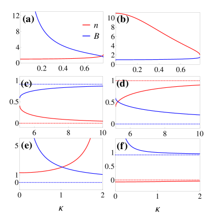
Figure 1: (Color online) Parameter configurations for $n_{\xi,\chi}^{(\pm)}$ and $B_{\xi,\chi}^{(\pm)}$ which yield the conserved spin quantity $\Sigma_{\xi}$ for $\theta=\chi\pi/4$ in case of a HH like ((a)-(d)) and LH like ((e)-(f)) ground state. The ratio between the Luttinger parameter $\gamma_{3}$ and $\gamma_{2}$ is set to $\Gamma=1.2$ and the linear Dresselhaus contribution is neglected, i.e., $\eta_{0}\rightarrow 0$. The domain for $\kappa$ is $A_{+}$ for $\xi=\chi$ and $A_{-}$ else. The dashed lines indicate the according asymptotes at large width of the quantum well. (a) $n_{\xi,\chi}^{(+)}$ and $B_{\xi,\chi}^{(+)}$, (b) $n_{\xi,\chi}^{(-)}$ and $B_{\xi,\chi}^{(-)}$ for $\xi=\chi=-1$. If $\xi=\chi=1$ holds only the sign of $n$ is inverted. (c) $n_{\xi,\chi}^{(+)}$ and $B_{\xi,\chi}^{(+)}$, (d) $n_{\xi,\chi}^{(-)}$ and $B_{\xi,\chi}^{(-)}$ for $\xi=-\chi=1$. Interchanging of $\xi$ and $\chi$ only changes the sign of $n$. (e) $n_{\xi,\chi}^{(+)}$ and $B_{\xi,\chi}^{(+)}$ which yield the conserved spin quantity $\Sigma_{-}$ for $\xi=\chi=-1$ and (f) $\xi=-\chi=-1$. The case $\xi=1$ reverses only the sign of $n$.

The domain $A_{-}$ ($\xi=-\chi$) shown in Fig. 1(c,d) is less realisic. Having large values of $\kappa$ implies a large width of the quantum well and a high Fermi energy which leads to populations in higher subbands where the model loses its validity. Also, for a large Fermi energy the Fermi contour is strongly deformed as can be understood by examining the term proportional to $\beta^{2}\gamma_{3}^{2}$ of the kinetic energy, Eq. (19). A spherical approximation becomes inappropriate. Moreover, if a strong strain is applied to the sample the appropriate model Hamiltonian needs to include also the coupling to the split-off band.

For future devices like the spin field-effect-transistor it is not only of interest to find persistent spin states. In fact, samples are favorable where the injected particles undergo only a well defined spin-rotation. Thereby the initial spin state, with $\bf k$ being a good quantum number, is not necessarily an eigenstate. Here, well defined means that the rotation only depends on the distance between the injection and detection position. For n-type systems this condition was already analyzed in Ref. Schliemann et al., 2003. Concerning a 2DHG as described in this paper, a spin-conserving condition which is valid for spin states with arbitrary wave vector cannot be found: The condition is limited to the averaged Fermi contour. For these states we can find an additional condition so that their precession depends only on the distance. At this, a necessary condition is an elastic scattering from impurities. The corresponding effective vector field in the case where the Eqs. (44,45) hold has the structure given by

$$\bm{\Omega}_{\text{HH}}={} (k_{x}+\xi k_{y})\varphi^{(\pm)}(k_{x},k_{y})\begin{pmatrix}\xi\\ 1\\ 0\end{pmatrix}\Bigg{|}_{k_{x}^{2}+k_{y}^{2}=k_{\parallel F}^{2}}.$$ (52)

In the case where $(k_{x}+\xi k_{y})\varphi^{\pm}(k_{x},k_{y})$ depends linearly on $k_{i}$ ($k_{\parallel F}$ is a constant), the mentioned spin-rotation is only distant dependent. Here, one finds

$$\varphi^{(\pm)}{} (k_{x},k_{y})$$

$$={} \frac{k_{\parallel F}^{2}\gamma_{2}\lambda_{R,+}}{\kappa^{2}(\pm\xi\chi\mathcal{W}+4\Gamma-\kappa^{2})}\Big{[}2(4\pm\xi\chi\mathcal{W})(1+\Gamma)$$

$$-(2\pm\xi\chi\mathcal{W}+6\Gamma)\kappa^{2}+\kappa^{4}+\xi 8(\Gamma^{2}-1)\kappa^{2}\frac{k_{x}k_{y}}{k_{\parallel F}^{2}}\Big{]}.$$ (53)

Thus, the special case where a well defined spin rotation occurs can only be found if $\Gamma\equiv\gamma_{3}/\gamma_{2}=\pm 1$.

III.2 Conserved Spin Quantity in Case of a LH Like Ground State

Analogously, it is possible to find conserved spin quantities if the ground state is LH like. Yet, the structure of the SO field is more complex since it contains additional first order term due to Dresselhaus SOC, Eq. (32). As stated above, an [110] uniaxial compressive strain leads to $\delta<0$ and therefore cannot be used. It is commonly known that for in-plane biaxial tensile stress LH ground state can be created, but in that case $\epsilon_{xy}$ vanishesSun et al. (2007). Consequently, combined strain effects are necessary to generate the required condition. Nonetheless, we stress that we do not demand a strong in-plane strain amplitude for identifying a conserved spin quantity. In fact, an appropriate tensor component $\epsilon_{zz}$ is necessary. This component is encapsulated in the splitting

$$\Delta_{\text{h1,ln}}={} \frac{\hbar^{2}}{2m_{0}}\braket{k_{z}^{2}}\left[\left(n^{2}-1\right)\gamma_{1}+2\left(n^{2}+1\right)\gamma_{2}\right]-\delta,$$ (54)

and thus in the SOC strength. For simplicity, we set $n\equiv n_{\text{LH}}$. Hence, the calculation of the conserved quantity is the same as before and valid as long as the deformation of the Fermi contour is not excessively strong. In this case, we find for the parameters $n_{\xi,\chi}^{(\pm)}$ and $B_{\xi,\chi}^{(\pm)}$ the relations

$$n_{\xi,\chi}^{(\pm)}=\frac{6\left(\Gamma-1\right)}{3\chi\Gamma\left(B_{\xi,\chi}^{(\pm)}\right)^{2}\kappa^{2}-2\xi\left(3\left(\Gamma+1\right)+2\mathcal{Q}\right)}$$ (55)

and

$$B_{\xi,\chi}^{(\pm)}=\sqrt{\frac{\xi\chi\left(4\mathcal{Q}-3\kappa^{2}+12\right)\pm\mathcal{P}}{6\Gamma\kappa^{2}}},$$ (56)

where we defined

$$\mathcal{P}={} \sqrt{16\left(\mathcal{Q}+3\Gamma\right)^{2}+24\kappa^{2}\left(\mathcal{Q}+6\Gamma-3\right)+9\kappa^{4}},$$ (57)

$$\mathcal{Q}={} \frac{\Delta_{\text{l1,h1}}}{\left|(\Delta_{\text{l1,h1}}\big{|}_{\delta=0})\right|}.$$ (58)

The parameters $n_{\xi,\chi}^{(\pm)}$ and $B_{\xi,\chi}^{(\pm)}$ are plotted in Fig. 1(e,f) for $\Gamma=1.2$ and $\mathcal{Q}=1$ which is equivalent to an energy shift $\delta=2\left|(\Delta_{\text{l1,h1}}\big{|}_{\delta=0})\right|$. We only find real solutions for $B_{\xi,\chi}^{(+)}$ and $n_{\xi,\chi}^{(+)}$. In contrast to the HH like ground state for a realistic system with $\Gamma>1$ we do not find a conserved spin quantity if strain is absent.

In the last part of this section we apply the insights on the conserved spin quantity to a prominent semiconductor.

III.3 Example: p-doped InSb

We choose p-doped InSb as an example to contrast the strained case yielding a conserved spin quantity with the one of a strainless sample. We assume a confinement in [001] direction with a depth of $L=$100\text{\,}\AA$$. To guarantee a low filling we set $k_{\parallel F}=$0.01\text{\,}\AA^{-1}$$. The used parameters here are listed in App. E. Further, we assume the additional splitting due to strain between HH and LH like subbands to vanish, $\delta=0$. Choosing an external electric field of $\mathcal{E}_{z}=$1.6\text{\,}\mathrm{k}\mathrm{V}\mathrm{/}\mathrm{c}\mathrm{m}$$ and a [110] tensile strain direction ($\epsilon_{xy}>0$), i.e., $\xi=\chi=1$, allows for a persistent spin polarization in [110] direction. Since we can assume a HH like ground state, we apply Eq. (44) and (45) and obtain the parameter for the in-plane strain strength to be $B_{1,1}^{(-)}=0.74$ and the corresponding ratio between Dresselhaus and Rashba SOC strength to be $n_{1,1}^{(-)}=-20.7$.

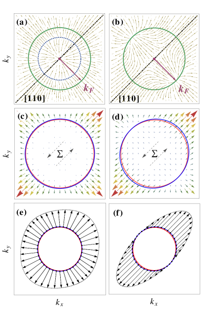
Figure 2: (Color online) Comparison of the SO field without applied strain (left column) and the case where strain gives rise to a conserved spin quantity $\Sigma$ in case of a HH like ground state. In the presented case the SOC strengths are $\lambda_{\text{D,+}}=$-42.5\text{\,}\mathrm{e}\mathrm{V}\AA^{3}$$, $\lambda_{\text{R,+}}=$2.05\text{\,}\mathrm{e}\mathrm{V}\AA^{3}$$ and $\eta_{+}=$-34.1\text{\times}{10}^{-3}\text{\,}\mathrm{e}\mathrm{V}\AA$$. (a) and (b) Stream plot of the effective SO vector field. The green circle indicates the axially symmetric Fermi contour. The blue dotted circle corresponds to $k_{0}=$6.9\text{\times}{10}^{-3}\text{\,}\AA^{-1}$$ where the field vanishes approximately. (c) and (d) Vector field and Fermi contours. The gray arrows indicate the spin polarization. (e) and (f) Detailed picture of the SO field that operates at the outer Fermi contour.

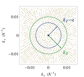
Figure 3: (Color online) Stream plot of the effective SO vector field without linear Dresselhaus contribution, i.e., $\eta_{+}\rightarrow 0$, in case of a HH like ground state. The strain-induced sources of the field move to a slightly lower Fermi wave vector by $\epsilon=$3.1\text{\times}{10}^{-3}\text{\,}\AA^{-1}$$ where the spin-preserving symmetry is recreated.

In Fig. 2(d) the resulting effective SO field is plotted and compared to the case where the [110] stress is absent, Fig. 2(c). A stream plot, Fig. 2(a,b) shows that without strain, Fig. 2(a), the vector field vanishes approximately at $k_{0}=$6.9\text{\times}{10}^{-3}\text{\,}\AA^{-1}$$ which is illustrated by the blue dotted circle. We see that even though the condition Eq. (49) on $n_{0}$ for the spin-preserving symmetry in the strainless case is not perfectly fulfilled, i.e., $n_{1,1}^{(-)}>n_{0}=-29.6$, the location where the field disappears is still well described by $k_{0}$ in Eq. (50). Additionally, there is one source in the vector field at $k_{\parallel}=0$. Including strain, Fig. 2(b), gives rise to two additional sources that are centered at the crossing of the Fermi contour and the $[1\overline{1}0]$ axis. This can be understood by considering the factor $(k_{x}+\xi k_{y})$ in Eq. (52). At these two sources vector field components are suppressed which are not collinear with the $[110]$ direction. The Fermi contours split due to the SOC. Without strain, they are only slightly deformed as consequence of the band warping. If strain is present, the deviation of rotational symmetry of the contours is enhanced. The deformation is most intense in the $[110]$ and $[1\overline{1}0]$ direction. To guide the viewer’s eye, we give in Fig. 2(e,f) a detailed picture of the SO field acting on the outer Fermi contour. In the case of strain the vectors lie parallel to the [110] direction. As discussed above, the plots also show that the preserved spin quantity is limited to the averaged Fermi contour. The vector field regions which are noncollinear are strongly suppressed, though. This leads to a reduction of spin relaxation even in the case of a general spin state injected into the 2DHG.

Influence of linear Dresselhaus terms

Moreover, we want to emphasize that in the chosen parameter regime the effect of the linear Dresselhaus contribution is only small. Fig. 3 shows how the field modifies if the linear Dresselhaus term proportional to $\eta_{+}$ is neglected. The strain-induced additional field sources move to a marginally lower Fermi wave vector by $\epsilon=$3.1\text{\times}{10}^{-3}\text{\,}\AA^{-1}$$ where the conserved spin quantity is reobtained. To first order in $\eta_{+}$ the shift $\epsilon$ can be generally estimated by

$$\epsilon={} \frac{\eta_{+}}{\sqrt{2}\beta\gamma_{3}}$$

$$\times\phantom{=}\left\{(\lambda_{\text{D,+}}+\lambda_{\text{R,+}})\left[\frac{\beta^{2}\lambda_{\text{D,+}}}{\braket{k_{z}^{2}}}+2(\lambda_{\text{D,+}}+\lambda_{\text{R,+}})\right]\right\}^{-1/2}.$$ (59)

We stress that the influence of the linear BIA terms becomes even smaller for increasing Fermi wave vector $k_{F}$ and in other materials such as GaAs is less significant.

IV Summary

Summarizing, we identified conserved spin quantities in a (001)-confined two-dimensional hole gas in semiconductors with zincblende structure. Thereby, we derived the dominant contribution to the SO field due to Rashba SOC directly from an electric field $\mathcal{E}_{z}$, which was missing in our previous publication, Ref. Dollinger et al., 2014. The significant effect due to Rashba SOC is only controlled by the subband gaps and not, as in the case of Dresselhaus SOC, by the conduction band gap. In view of recent publications, we also included the effect of linear Dresselhaus SOC terms whose significance was pointed out in Refs. Durnev et al., 2014; Luo et al., 2010 to be underestimated. The proper determination of the SO field enabled us to conclude that there are two possiblities for long-lived spin states. In respect of an unstrained sample such states exist only for heavy holes. It requires a certain ratio of cubic Rashba and Dresselhaus SOC strength defined solely by the Luttinger parameters $\gamma_{2}$ and $\gamma_{3}$. Other spin-preserving symmetries occur in presence of strain for both a HH like and LH like ground state. Here, a non-vanishing [110] shear strain component $\epsilon_{xy}$ and a symmetric in-plane normal strain $\epsilon_{xx}=\epsilon_{yy}$ are essential. We have recovered the conserved spin quantity presented in Ref. Sacksteder and Bernevig, 2014 for the special case where $\gamma_{2}/\gamma_{3}=-1$. In all circumstances, owing to the presence of both linear and cubic terms due to SOC the persistent spin states are bound to a Fermi contour. We have also demonstrated that only for this case and for $\gamma_{2}/\gamma_{3}=1$ one finds a spin rotation of a spin on the averaged Fermi contour which only dependents on the distance between the injection and detection position. Moreover, we have shown that for the existence of a conserved spin quantity in semiconductors which are accessible for experiments (e.g., systems with $\gamma_{2}/\gamma_{3}\approx 1$) the interplay between Dresselhaus SOC, Rashba SOC and possibly strain is crucial.

In this way, shear strain has turned out to be a key component for an efficient manipulation of spin lifetime in 2D hole systems of zincblende structure.

Appendix A Luttinger Parameter Relation

Here, we shortly focus on the Luttinger parameters $\gamma_{2}$ and $\gamma_{3}$. The warping of the valence band is directly proportional to their difference. Comparing with experimental results, for most semiconductors one finds the parameter $\gamma_{3}$ to be larger than $\gamma_{2}$.Vurgaftman et al. (2001); Yu and Cardona (2010); Winkler (2003) This becomes clear when describing the system using ${\bf k\cdot p}$ method for band structure calculations, which yields the relation

$$\gamma_{3}-\gamma_{2}=\frac{2}{3m_{0}E_{0}^{\prime}}Q^{2}.$$ (60)

Hereby, we follow the notation and phase conventions of Ref. Yu and Cardona, 2010 where $Q\in\mathbb{R}$ and $iQ$ being a momentum matrix element between the $\Gamma_{8v}$ valence and the $\Gamma_{7c}$ and $\Gamma_{8c}$ conduction band states. The energy separation between the conduction band $\Gamma_{7c}$ and the $j=3/2$ valence bands is denoted as $E_{0}^{\prime}>0$.Yu and Cardona (2010)

Appendix B Applied Approximations

B.1 Löwdin’s Partitioning

In this paper we start with a Hamiltonian which describes HH and LH in the bulk. At the $\Gamma$ point both types are degenerate. Imposing a confinement on the system reduces it to a quasi 2D system, generating HH like and LH like subbands. The simplification, which allows for further analytical studies, is now to focus on the subspace spanned by either the set $\{\ket{j=3/2,m_{j}=\pm 1/2}\ket{n=1}\}$ or $\{\ket{j=3/2,m_{j}=\pm 3/2}\ket{n=1}\}$, only, where $n$ is the subband index. Let us call this subset $A$. Due to the confinement in growth direction and strain, this subset is well separated in energy at the $\Gamma$ point from all other subbands (except the particular case where strain is exactly reversing the energy splitting due to the confinement between the lowest band and the subsequent one at the $\Gamma$ point). Assuming $A$ having HH character, let us call the subset spanned by $\{\ket{j=3/2,m_{j}=\pm 3/2}\ket{(n>1)},$ $\ket{j=3/2,m_{j}=\pm 1/2}\ket{n}\}$ subset $B$. To end up with an effective model which focuses on the lowest HH(LH) like subbands, one treats the effect of subset $B$ on the subset $A$ in a perturbative manner. Here, one has to distinguish between degenerate and non-degenerate perturbation theory since $A$ and $B$ may contain exact or approximate degeneracies. Applying the quasi-degenerate perturbation theory, also called Löwdin’s partitioning, avoids this tricky task. It is described in great detail in the book by Bir and PikusBir and Pikus (1974) or by WinklerWinkler (2003). With the subspace decomposition of our problem in mind, we give in the following a short formal description of the perturbation procedure. Assume that $\mathcal{H}$ can be expressed as a sum of a Hamiltonian $\mathcal{H}^{0}$ with known eigenvalues $E_{n}$ and eigenfunctions $\ket{\psi_{n}}$ and $\mathcal{H^{\prime}}$ which is treated as a perturbation. Further, assume $\mathcal{H^{\prime}}$ being a sum of a block diagonal matrix $\mathcal{H}^{1}$ with subsets $A$ and $B$ and $\mathcal{H}^{2}$ describing the coupling of both subsystems,

$$\mathcal{H}=\mathcal{H}^{0}+\mathcal{H^{\prime}}=\mathcal{H}^{0}+\mathcal{H}^{1}+\mathcal{H}^{2}.$$ (61)

In accordance with Ref. Winkler, 2003; Bir and Pikus, 1974, we define the indices $m,m^{\prime},m^{\prime\prime}$ corresponding to the states in set $A$, the indices $l,l^{\prime},l^{\prime\prime}$ to states in set $B$ and the matrix elements between them as

$$\mathcal{H}^{\prime}_{ij}=\braket{\psi_{i}}{\mathcal{H}^{\prime}}{\psi_{j}}.$$ (62)

Now one can find a non-block-diagonal anti-Hermitian matrix $S$ which allows for a transformation of $\mathcal{H}$ yielding a block diagonal Hamiltonian $\widetilde{\mathcal{H}}=e^{-S}\mathcal{H}e^{S}$. $S$ and thus $\mathcal{H}$ can be found from a successive approximation. The first terms

$$\widetilde{\mathcal{H}}={} \mathcal{H}^{(0)}+\mathcal{H}^{(1)}+\mathcal{H}^{(2)}+\mathcal{H}^{(3)}+\ldots$$ (63)

are given by

$$\mathcal{H}^{(0)}_{mm^{\prime}}={} \mathcal{H}^{0}_{mm^{\prime}}\,,$$ (64)

$$\mathcal{H}^{(1)}_{mm^{\prime}}={} \mathcal{H}^{\prime}_{mm^{\prime}}\,,$$ (65)

$$\mathcal{H}^{(2)}_{mm^{\prime}}={} \frac{1}{2}\sum_{l}\mathcal{H}^{\prime}_{ml}\mathcal{H}^{\prime}_{lm^{\prime}}\left[\frac{1}{E_{m}-E_{l}}+\frac{1}{E_{m^{\prime}}-E_{l}}\right],$$ (66)

$$\mathcal{H}^{(3)}_{mm^{\prime}}={} -\frac{1}{2}\sum_{l,m^{\prime\prime}}\left[\frac{\mathcal{H}^{\prime}_{ml}\mathcal{H}^{\prime}_{lm^{\prime\prime}}\mathcal{H}^{\prime}_{m^{\prime\prime}m^{\prime}}}{(E_{m^{\prime}}-E_{l})(E_{m^{\prime\prime}}-E_{l})}\right.$$

$$\phantom{-\frac{1}{2}\sum_{l,m^{\prime\prime}}}+\left.\frac{\mathcal{H}^{\prime}_{mm^{\prime\prime}}\mathcal{H}^{\prime}_{m^{\prime\prime}l}\mathcal{H}^{\prime}_{lm^{\prime}}}{(E_{m}-E_{l})(E_{m^{\prime\prime}}-E_{l})}\right]$$

$$+\frac{1}{2}\sum_{l,l^{\prime}}\mathcal{H}^{\prime}_{ml}\mathcal{H}^{\prime}_{ll^{\prime}}\mathcal{H}^{\prime}_{l^{\prime}m^{\prime}}\left[\frac{1}{(E_{m}-E_{l})(E_{m}-E_{l^{\prime}})}\right.$$

$$\phantom{-\frac{1}{2}\sum_{l,m^{\prime\prime}}}\left.+\frac{1}{(E_{m^{\prime}}-E_{l})(E_{m^{\prime}}-E_{l^{\prime}})}\right].$$ (67)

Note that each of the subsets $A$ and $B$ may be degenerate but it is crucial that the subsets are chosen to be separated in energy, i.e., $E_{m}\neq E_{l}$.

B.2 Dominant Invariants for the Cubic BIA Spin Splitting in Bulk Semiconductors

Our starting point is the extended Kane model excluding contributions from remote bands, i.e., $C_{k}=0$. The remaining invariants for the $\Gamma_{8v}$ band block in this model, which give rise to cubic BIA spin splitting, are given by Eq. (3). In order to determine the coefficients, Löwdin’s partitioning in the energy gaps at the $\Gamma$ point in the extended Kane model can be applied. In Ref. Winkler, 2003 [Tab.6.3.], the coefficients in third order perturbation theory have been listed for several compounds. It reveals that in the bulk compared to $b_{41}^{8v8v}$, the terms proportional to $b_{42}^{8v8v}$, $b_{51}^{8v8v}$ and $b_{52}^{8v8v}$ can be neglected. As an example, we compare the extended Kane model with the effective $4\times 4$ model used in this paper by calculating the absolute value $|\Delta E|$. The latter is the BIA spin splitting calculated for both LH and HH states in GaAs for ${\bf k}||[110]$ in the bulk system. The result is plotted in Fig. 4 and shows very good agreement between both models. Deviations are only present at large $k$ values.

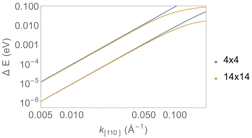
Figure 4: (Color online) Absolute value $|\Delta E|$ of the BIA spin splitting of LH and HH states in GaAs for ${\bf k}||[110]$ in the bulk system. The results are obtained by means of diagonalization of the full $14\times 14$ matrix of the extended Kane model (orange) and the effective $4\times 4$ model used in this paper (blue), following Ref. Winkler, 2003. Here, contributions from remote bands to the extended Kane model are excluded.

Note, however, that for a certain choice of parameters for the ${\bf k}\cdot{\bf p}$ model higher order corrections to the coefficients can be significant, as recently shown in Ref. Durnev et al., 2014. For a comparison of ${\mathcal{H}}_{\text{BIA}}$ with the terms used in Ref. Rashba and Sherman, 1988 or Ref. Durnev et al., 2014 it is useful to recast Eq. (3) for $C_{k}=0$ in the form

$${\mathcal{H}}_{\text{BIA}}={} b_{41}^{8v8v}({\bf J}\cdot{\bm{\kappa}})+b_{42}^{8v8v}\sum_{\alpha}J_{\alpha}^{3}\kappa_{\alpha}+(b_{52}^{8v8v}-b_{51}^{8v8v})$$

$$\times\sum_{\alpha}V_{\alpha}k_{\alpha}\left(k_{\alpha}^{2}+\frac{1}{(b_{52}^{8v8v}/b_{51}^{8v8v})-1}k^{2}\right),$$ (68)

with $V_{x}=\{J_{x},J_{y}^{2}-J_{z}^{2}\}$, $J_{\alpha}$ and $\kappa_{x}=k_{x}(k_{y}^{2}-k_{z}^{2})$ (and corresponding terms). The relation between the coefficients used in Ref. Rashba and Sherman, 1988 and the one in Eq. (3) are thus given by

$$b_{41}^{8v8v}=\frac{i}{6}PP^{\prime}Q\frac{1}{E_{0}}\left(\frac{13}{E^{\prime}_{0}}-\frac{5}{E^{\prime}_{0}+\Delta_{0}^{\prime}}\right)\hat{=}{} \,\alpha_{v}+\frac{13}{8}\delta\alpha_{v},$$ (69)

$$b_{42}^{8v8v}=\frac{2i}{3}PP^{\prime}Q\frac{1}{E_{0}}\left(\frac{1}{E^{\prime}_{0}}-\frac{1}{E^{\prime}_{0}+\Delta_{0}^{\prime}}\right)\hat{=}{} -\frac{1}{2}\delta\alpha_{v},$$ (70)

$$b_{51}^{8v8v}=\frac{2i}{9}PP^{\prime}Q\frac{1}{E_{0}}\left(\frac{1}{E^{\prime}_{0}+\Delta_{0}^{\prime}}-\frac{1}{E_{0}^{\prime}}\right)\hat{=}{} -\frac{1}{6}\delta\alpha_{v}$$ (71)

$$b_{52}^{8v8v}=\frac{4i}{9}PP^{\prime}Q\frac{1}{E_{0}}\left(\frac{1}{E_{0}^{\prime}}-\frac{1}{E^{\prime}_{0}+\Delta_{0}^{\prime}}\right)\hat{=}{} \frac{1}{3}\delta\alpha_{v},$$ (72)

with

$$P={} \frac{\hbar}{m_{0}}\braket{S}{p_{x}}{X},$$ (73)

$$P^{\prime}={} \frac{\hbar}{m_{0}}\braket{S}{p_{x}}{X^{\prime}},$$ (74)

$$Q={} \frac{\hbar}{m_{0}}\braket{X}{p_{y}}{Z^{\prime}}$$ (75)

and

$$\Delta_{0}={} -\frac{3i\hbar}{4m_{0}^{2}c^{2}}\braket{X}{[(\nabla V_{0})\times{\bf p}]_{y}}{Z},$$ (76)

$$\Delta_{0}^{\prime}={} -\frac{3i\hbar}{4m_{0}^{2}c^{2}}\braket{X^{\prime}}{[(\nabla V_{0})\times{\bf p}]_{y}}{Z^{\prime}},$$ (77)

$$\Delta^{-}={} -\frac{3i\hbar}{4m_{0}^{2}c^{2}}\braket{X}{[(\nabla V_{0})\times{\bf p}]_{y}}{Z^{\prime}},$$ (78)

with $V_{0}$ the Coulomb potential of the atomic core, $(X,Y,Z)$ the topmost bonding p-like valence band states and the antibonding s-like (S) and p-like $(X^{\prime},Y^{\prime},Z^{\prime})$ states in the lowest conduction band.

Notice that there is a difference in the application of perturbation theory to get the prefactors: According to Eq. [19a] in Ref. Pikus et al., 1988, e.g., one finds for $\Delta_{0}^{\prime}\approx 0$ the term, which corresponds to $b_{42}^{8v8v}$, to be

$$b_{42}^{8v8v}\sim PP^{\prime}Q\frac{1}{E_{0}(E_{0}+E_{0}^{\prime})}.$$ (79)

In contrast, Eq.(70) vanishes if $\Delta_{0}^{\prime}$ can be neglected.

B.3 LH like Valence Band Ground State: Mixing of the Electric Field and Dresselhaus Term

Assuming a LH like valence band ground state and applying Löwdin perturbation to third order, terms appear in third order which couple the electric field $\mathcal{E}_{z}$ with the Dresselhaus term proportional to $b_{41}^{8v8v}$,

$$\Omega_{\text{mix},x}^{(3)}={} -\frac{256e\mathcal{E}_{z}b_{41}^{8v8v}}{27\Delta_{\text{l1,l2}}^{2}}\left(2b_{41}^{8v8v}k_{y}(k_{x}^{2}-k_{y}^{2})+e\mathcal{E}_{z}k_{x}\right),$$

$$\Omega_{\text{mix},y}^{(3)}={} -\frac{256e\mathcal{E}_{z}b_{41}^{8v8v}}{27\Delta_{\text{l1,l1}}^{2}}\left(2b_{41}^{8v8v}k_{y}(k_{x}^{2}-k_{y}^{2})-e\mathcal{E}_{z}k_{x}\right),$$

$$\Omega_{\text{mix},z}^{(3)}={} 0.$$ (80)

It is negligible if compared to those proportional to $\lambda_{\text{R},\pm}$, $\lambda_{\text{D},\pm}$ or $\eta_{-}$, Eqs. (24)-(27), since we assume the SOC to be a small correction. Therefore, we neglect these terms in the calculation of the conserved spin quantity.

Appendix C Domain

If the $C_{k}$ term in Eq. 23 cannot be neglected the real solutions for $B_{\xi,\chi}^{(\pm)}$ are only found for $\kappa\in A_{\mathrm{sgn}(\xi\cdot\chi)}$ where

$$A_{+}={} \left[0,2\sqrt{1+2\Gamma+\frac{\sqrt{3}}{2}\frac{C_{k}}{\tilde{\lambda}_{\text{D}}}(1+\Gamma)-2\sqrt{\left(1+\Gamma\right)\Lambda}}\right],$$ (81)

$$A_{-}={} \left[2\sqrt{1+2\Gamma+\frac{\sqrt{3}}{2}\frac{C_{k}}{\tilde{\lambda}_{\text{D}}}(1+\Gamma)+2\sqrt{\left(1+\Gamma\right)\Lambda}},\infty\right)$$ (82)

$$\text{with }\Lambda={} \frac{1}{2\tilde{\lambda}_{\text{D}}^{2}}(6C_{k}^{2}(1+\Gamma)+8\sqrt{3}C_{k}\tilde{\lambda}_{\text{D}}(1+2\Gamma)$$ (83)

$$+\tilde{\lambda}_{\text{D}}(3k_{\parallel F}^{2}(b_{42}^{8v8v}+b_{51}^{8v8v})+32\Gamma\tilde{\lambda}_{\text{D}}))$$ (84)

$$\text{and }\tilde{\lambda}_{\text{D}}={} \gamma_{2}k_{\parallel F}^{2}\lambda_{\text{D},+}.$$ (85)

Appendix D Strain

D.1 Deformation Potentials

The deformation potentials $a$, $b$ and $d$ can be defined in different ways and there are several of them in the literature. We list some relations between different definitions in Tab. 1.

Eq. (4), Ref. Sacksteder and Bernevig,2014	Ref. Winkler,2003	Ref. Bir and Pikus, 1974,Sun et al., 2007,Sun et al., 2010,Yu and Cardona, 2010
$a$	$D_{d}-\frac{5}{6}D_{u}$	$a+\frac{5}{4}b$
$b$	$\frac{2}{3}D_{u}$	$-b$
$d$	$\frac{2}{3}D_{u}^{\prime}$	$-d/\sqrt{3}$

Table 1: Relations between different conventions for the deformation potentials for the $\Gamma_{8v}$ valence band.

D.2 Uniaxial Strain via Piezo Crystals

Experimentally an unaxial strain can be conveniently implemented by the application of a piezo crystal since the deformation is tunable. In this setup, as done by Habib et al. in Ref. Habib et al., 2007, the sample is fixed at one side of the piezo crystal where we align the poling direction of the piezo with the [110] direction. Depending on the polarity of the applied voltage, the piezo crystal extends (shrinks) along its poling direction and simultaneously shrinks (extends) perpendicular to it. Assuming the deformation being completely transmitted to the sample, we can relate the strain coefficients of the sample, where the principal axes correspond to the three $\left\langle 100\right\rangle$ axes, to the strain coefficients of the piezo, which can be directly measured. We define the transfered strain parallel to the poling and perpendicular to it as $\epsilon^{\prime}_{\parallel}$ and $\epsilon^{\prime}_{\perp}$. Since due to Hooke’s law an in-plane strain generates also a finite out-of-plane component, the strain tensor of the sample becomes

$$\bm{\epsilon}=\frac{1}{2}\begin{pmatrix}\epsilon^{\prime}_{\parallel}+\epsilon^{\prime}_{\perp}&\epsilon^{\prime}_{\parallel}-\epsilon^{\prime}_{\perp}&0\\ \epsilon^{\prime}_{\parallel}-\epsilon^{\prime}_{\perp}&\epsilon^{\prime}_{\parallel}+\epsilon^{\prime}_{\perp}&0\\ 0&0&-\frac{2C_{12}}{C_{11}}\left(\epsilon^{\prime}_{\parallel}+\epsilon^{\prime}_{\perp}\right)\end{pmatrix},$$ (86)

where $C_{12}$ and $C_{11}$ are stiffness tensor components depending on the sample’s material. It becomes clear that in this situation the in-plane normal strain is symmetric, i.e., $\epsilon_{xx}=\epsilon_{yy}$, and the shear strain component $\epsilon_{xy}\neq 0$ as $\epsilon^{\prime}_{\parallel}$ and $\epsilon^{\prime}_{\perp}$ have opposite sign, which corresponds to the situation demanded in Sec. III.

Appendix E BIA Parameters

In Tab. 2 we list the coefficients for the invariants appearing in the BIA Hamiltonian, Eq. (3), for some common compounds (all values in eVų, except for $C_{k}$ in eVÅ)Winkler (2003).

	GaAs	AlAs	InSb
$C_{k}$	-0.0034	0.0020	-0.0082
$b_{41}^{8v8v}$	-81.93	-33.51	-934.8
$b_{42}^{8v8v}$	1.47	0.526	41.73
$b_{51}^{8v8v}$	0.49	0.175	13.91
$b_{52}^{8v8v}$	-0.98	-0.35	-27.82

Table 2: Expansion coefficients for the invariants in the used model, Eq. (3), up to third order in ${\bf k}$ which give rise to BIA spin splitting. All values in eVų, except for $C_{k}$ in eVÅ.Winkler (2003)

References

- Datta and Das (1990) S. Datta and B. Das, Appl. Phys. Lett. 56, 665 (1990).
- D’yakonov and Perel’ (1971) M. I. D’yakonov and V. I. Perel’, Fiz. Tverd. Tela 13, 3581 (1971), [Sov. Phys. Solid State 13, 3023 (1972)].
- Noether (1918) E. Noether, Nachr. Konig. Gesellsch. Wiss. Gottingen, Math-Phys. Klasse 1918, 235 (1918).
- Dresselhaus (1955) G. Dresselhaus, Phys. Rev. 100, 580 (1955).
- Rashba (1960) E. I. Rashba, Sov. Phys.-Solid State 2, 1109 (1960).
- J. Ohkawa and Uemura (1974) F. J. Ohkawa and Y. Uemura, J. Phys. Soc. Jpn. 37, 1325 (1974).
- Schliemann et al. (2003) J. Schliemann, J. C. Egues, and D. Loss, Phys. Rev. Lett. 90, 146801 (2003).
- Bernevig et al. (2006) B. A. Bernevig, J. Orenstein, and S.-C. Zhang, Phys. Rev. Lett. 97, 236601 (2006).
- Koralek et al. (2009) J. D. Koralek, C. P. Weber, J. Orenstein, B. A. Bernevig, S.-C. Zhang, S. Mack, and D. D. Awschalom, Nature 458, 610 (2009).
- Walser et al. (2012) M. P. Walser, C. Reichl, W. Wegscheider, and G. Salis, Nat Phys 8, 757 (2012).
- Rashba and Sherman (1988) E. Rashba and E. Sherman, Phys. Lett. A 129, 175 (1988).
- Sun et al. (2010) Y. Sun, S. E. Thompson, and T. Nishida, Strain Effects in Semiconductors: Theory and Device Applications (Springer, 2010).
- Sun et al. (2007) Y. Sun, S. E. Thompson, and T. Nishida, J. Appl. Phys. 101, 104503 (2007).
- Seiler et al. (1977) D. G. Seiler, B. D. Bajaj, and A. E. Stephens, Phys. Rev. B 16, 2822 (1977).
- Cardona et al. (1988) M. Cardona, N. E. Christensen, and G. Fasol, Phys. Rev. B 38, 1806 (1988).
- Korn et al. (2010) T. Korn, M. Kugler, M. Griesbeck, R. Schulz, A. Wagner, M. Hirmer, C. Gerl, D. Schuh, W. Wegscheider, and C. Schüller, New J. Phys. 12, 043003 (2010).
- Kugler et al. (2009) M. Kugler, T. Andlauer, T. Korn, A. Wagner, S. Fehringer, R. Schulz, M. Kubová, C. Gerl, D. Schuh, W. Wegscheider, P. Vogl, and C. Schüller, Phys. Rev. B 80, 035325 (2009).
- Hirmer et al. (2011) M. Hirmer, M. Hirmer, D. Schuh, W. Wegscheider, T. Korn, R. Winkler, and C. Schüller, Phys. Rev. Lett. 107, 216805 (2011).
- Grbić et al. (2008) B. Grbić, R. Leturcq, T. Ihn, K. Ensslin, D. Reuter, and A. D. Wieck, Phys. Rev. B 77, 125312 (2008).
- Sacksteder and Bernevig (2014) V. E. Sacksteder and B. A. Bernevig, Phys. Rev. B 89, 161307 (2014).
- Dollinger et al. (2014) T. Dollinger, M. Kammermeier, A. Scholz, P. Wenk, J. Schliemann, K. Richter, and R. Winkler, Phys. Rev. B 90, 115306 (2014).
- Vurgaftman et al. (2001) I. Vurgaftman, J. R. Meyer, and L. R. Ram-Mohan, J. Appl. Phys. 89, 5815 (2001).
- Yu and Cardona (2010) P. Yu and M. Cardona, Fundamentals of Semiconductors: Physics and Materials Properties, Graduate Texts in Physics (Springer, 2010).
- Winkler (2003) R. Winkler, Spin-Orbit Coupling Effects in Two-Dimensional Electron and Hole Systems, Springer Tracts in Modern Physics, Vol. 191 (Springer-Verlag, Berlin, 2003).
- Note (1) A negative value of appears, e.g., when the lowest conduction band is not an s-type band as it is the case in diamondWillatzen et al. (1994). However, for diamond one finds only Willatzen et al. (1994).
- Bulaev and Loss (2005) D. V. Bulaev and D. Loss, Phys. Rev. Lett. 95, 076805 (2005).
- Luo et al. (2010) J.-W. Luo, A. N. Chantis, M. van Schilfgaarde, G. Bester, and A. Zunger, Phys. Rev. Lett. 104, 066405 (2010).
- Durnev et al. (2014) M. V. Durnev, M. M. Glazov, and E. L. Ivchenko, Phys. Rev. B 89, 075430 (2014).
- Luttinger (1956) J. M. Luttinger, Phys. Rev. 102, 1030 (1956).
- Bir and Pikus (1974) G. L. Bir and G. E. Pikus, Symmetry and Strain-Induced Effects in Semiconductors (Wiley/Halsted Press, 1974).
- Ivchenko and Pikus (1995) E. Ivchenko and P. Pikus, Superlattices and Other Heterostructures: Symmetry and Optical Phenomena, Springer Series in Solid-State Science 110 (Springer, 1995).
- Ivchenko et al. (1996) E. L. Ivchenko, A. Y. Kaminski, and U. Rössler, Phys. Rev. B 54, 5852 (1996).
- Magri and Zunger (2000) R. Magri and A. Zunger, Phys. Rev. B 62, 10364 (2000).
- Note (2) Note that the definition in Eq. (14) differs from the one given in Ref. \rev@citealpnumPhysRevB.89.161307 in the term proportional to by a factor of .
- Kane (1957) E. O. Kane, J. Phys. Chem. Solids 1, 249 (1957).
- Habib et al. (2007) B. Habib, J. Shabani, E. P. De Poortere, M. Shayegan, and R. Winkler, Phys. Rev. B 75, 153304 (2007).
- Knap et al. (1996) W. Knap, C. Skierbiszewski, A. Zduniak, E. Litwin-Staszewska, D. Bertho, F. Kobbi, J. L. Robert, G. E. Pikus, F. G. Pikus, S. V. Iordanskii, V. Mosser, K. Zekentes, and Y. B. Lyanda-Geller, Phys. Rev. B 53, 3912 (1996).
- Dollinger (2013) T. Dollinger, Spin Transport in Two-Dimensional Electron and Hole Gases, Ph.D. thesis, Universität Regensburg (2013).
- Kettemann (2007) S. Kettemann, Phys. Rev. Lett. 98, 176808 (2007).
- Note (3) Eq. (60) is valid if the reduced Luttinger parameters and in the applied model vanishMayer and Rössler (1991).
- Note (4) Following the Koster notationKoster (1957), one has for the tetrahedral point group three double group representations given by the two two-dimensional representations , and the four dimensional one .
- Pikus et al. (1988) G. Pikus, V. Maruschak, and A. Titkov, Fiz. Tekh. Poluprovodn. 23 (1988).
- Willatzen et al. (1994) M. Willatzen, M. Cardona, and N. E. Christensen, Phys. Rev. B 50, 18054 (1994).
- Mayer and Rössler (1991) H. Mayer and U. Rössler, Physical Review B 44, 9048 (1991).
- Koster (1957) G. Koster, in Solid State Physics, Vol. 5, edited by F. Seitz and D. Turnbull (Academic Press, 1957) pp. 173 – 256.