First order constrained optimization algorithms with feasibility updates

Abstract.

We propose first order algorithms for convex optimization problems where the feasible set is described by a large number of convex inequalities that is to be explored by subgradient projections. The first algorithm is an adaptation of a subgradient algorithm, and has convergence rate $1/\sqrt{k}$. The second algorithm has convergence rate $1/k$ when (1) one has linear metric inequality in the feasible set, (2) the objective function is strongly convex, differentiable and has Lipschitz gradient, and (3) it is easy to optimize the objective function on the intersection of two halfspaces. This second algorithm generalizes Haugazeau’s algorithm. The third algorithm adapts the second algorithm when condition (3) is dropped. We give examples to show that the second algorithm performs poorly when the objective function is not strongly convex, or when the linear metric inequality is absent.

1. Introduction

Let $f:\mathbb{R}^{n}\to\mathbb{R}$ and $f_{j}:\mathbb{R}^{n}\to\mathbb{R}$, where $j\in\{1,\dots,m\}$, be convex functions. Let $Q\subset\mathbb{R}^{n}$ be a closed convex set. The problem that we study in this paper is

$$\min f(x)$$

s.t. $$f_{j}(x)\leq 0\mbox{ for }j\in\{1,\dots,m\}$$

$$x\in Q.$$

If $m$ is large, then it might be difficult for an algorithm to find an $x$ satisfying the stated constraints, let alone solve the optimization problem. We now recall material relevant with our approach for trying to solve (1).

1.1. Projection methods for solving feasibility problems

For finitely many closed convex sets $C_{1},\dots,C_{m}$ in $\mathbb{R}^{n}$, the Set Intersection Problem (SIP) is stated as:

$$\mbox{(SIP):}\quad\mbox{Find }x\in C:=\bigcap_{j=1}^{m}C_{j}\mbox{, where }C\neq\emptyset.$$ (1.2)

The SIP is also referred to as feasibility problems in the literature. When $m$ is large, the Method of Alternating Projections (MAP) is a reasonable way to solve the SIP. As its name suggests, the MAP finds the sequence $\{x_{k}\}_{k=1}^{\infty}$ by projecting onto the $C_{j}$ cyclically, i.e., $x_{k+1}=P_{C_{k^{\prime}}}(x_{k})$, where $k^{\prime}$ is the number in $\{1,\dots,m\}$ such that $m$ divides $k-k^{\prime}$. We refer the reader to [BB96, BR09, ER11], as well as [Deu01, Chapter 9] and [BZ05, Subsubsection 4.5.4], for more on the literature of using projection methods to solve the SIP.

The convergence rate of the MAP is linear under the assumption of linear regularity. The notion was introduced and studied by [Bau96] (Definition 4.2.1, page 53) in a general setting of a Hilbert space. See also [BB96] (Definition 5.6, page 40). Recently, it has been studied in [DH06a, DH06b, DH08]. The connection with the stability under perturbation of the sets $C_{j}$ is investigated in [Kru04, Kru06] and other works.

Another problem closely related to the SIP is the Best Approximation Problem (BAP), stated as

(BAP): $$\underset{x\in X}{\min} \frac{1}{2}\|x-x_{0}\|^{2}$$

s.t. $$x\in C:=\bigcap_{j=1}^{m}C_{j}.$$

In other words, the BAP is the problem of finding the projection of $x_{0}$ onto $C$. The BAP follows the template of (1) when $f(x)=\frac{1}{2}\|x-x_{0}\|^{2}$, $f_{j}(x)=d(x,C_{j})$ for each $j\in\{1,\dots,m\}$, and $Q=\mathbb{R}^{n}$. Dykstra’s algorithm [Dyk83, BD85] is a projection algorithm for solving the BAP. It was rediscovered in [Han88] using mathematical programming duality. Another algorithm is Haugazeau’s algorithm [Hau68] (see [BC11]). The convergence rate of Dykstra’s algorithm has been analyzed in the polyhedral case [DH94, Xu00], but little is known about the general convergence rates of Dykstra’s and Haugazeau’s Algorithms.

For more on the background and recent developments of the MAP and its variants, we refer the reader to [BB96, BR09, ER11], as well as [Deu01, Chapter 9] and [BZ05, Subsubsection 4.5.4].

1.2. First order algorithms and algorithms for (1)

First order methods in optimization are methods based on function values and gradient evaluations. Even though first order methods have a slower rate of convergence than other algorithms, the advantage of first order algorithms is that each iteration is easy to perform. For large scale problems, algorithms with better complexity require too much computational effort to perform each iteration, so first order algorithms can be the only practical method. Classical references include [NY83, Nes83, Nes84, Nes89], and newer references include [Nes04, JN11a, JN11b]. See also [BT09].

As far as we are aware, the problem (1) where projections are used to address the feasibility of solutions are studied in [Ned11, WB15]. In both papers, the approach is to use random projection methods, while the second paper focuses on the generalized setting of variational inequalities.

1.3. Contributions of this paper

In Section 3, we modify the subgradient algorithm in [Nes04, Section 3.2.4] for solving (1) so that the new algorithm is more suitable for solving the problem (1) when $m$ is large. When the functions $\{f_{j}\}_{j=1}^{m}$ satisfy the linear metric inequality property in Definition 2.4, we show that projection methods can be used instead. The algorithms in this section have $O(1/\sqrt{k})$ convergence rate to the optimal objective value, just like the subgradient algorithm.

The convergence of projection algorithms for the SIP (1.2) is linear when a linear metric inequality condition is satisfied. Furthermore, the convergence of first order algorithms for strongly convex functions with Lipschitz gradient to the objective value and the unique optimal solution is linear. It is therefore natural to look at the convergence rate of (1) when

1. the functions $\{f_{j}\}_{j=1}^{m}$ satisfy linear metric inequality, and

2. $f(\cdot)$ is strongly convex, differentiable and has Lipschitz gradient.

In Section 4, we generalize Haugazeau’s algorithm to obtain a first order algorithm to solve (1) for the case when (1) and (2) are satisfied, and

1. $f(\cdot)$ is structured enough to optimize over the intersection of two halfspaces.

Our algorithms have a $O(1/k)$ convergence rate to the optimal objective value and $O(1/\sqrt{k})$ convergence to the optimizer. We believe that such a convergence rate for Haugazeau’s algorithm is new.

In Section 5, we propose a first order algorithm to solve (1) when (1) and (2) are satisfied, but not (3). The convergence rate to the optimal objective value and to the optimizer are slightly worse than the algorithms in Section 4.

In Section 6, we show that in the case where the dimension and number of constraints are large, then a $(1/k)$ convergence rate is best possible for strongly convex problems in a model generalizing Haugazeau’s algorithm, while an arbitarily slow convergence rate applies when there is convexity but no strong convexity in the objective function.

In Section 7, we show that the $O(1/k)$ rate of convergence of Haugazeau’s algorithm to the objective value occurs even for a very simple example. We give a second example to show that Haugazeau’s algorithm converges arbitrarily slowly in the absence of linear metric inequality.

2. Preliminaries

In this section, we recall some results that will be necessary for the understanding of this paper. We start with strongly convex functions.

Definition 2.1.

(Strongly convex functions) We say that $f:\mathbb{R}^{n}\to\mathbb{R}$ is strongly convex with convexity parameter $\mu$ if

$$f(y)\geq f(x)+\langle f^{\prime}(x),y-x\rangle+\frac{\mu}{2}\|x-y\|^{2}\mbox{ for all }x,y\in\mathbb{R}^{n}.$$

Denote the set $\mathcal{S}_{\mu,L}^{1,1}$ to be the set of all functions $f:\mathbb{R}^{n}\to\mathbb{R}$ such that $f(\cdot)$ is strongly convex with parameter $\mu$ and $f^{\prime}(\cdot)$ is Lipschitz with constant $L$.

We recall some standard results and notation on the method of alternating projections that will be used in the rest of the paper.

Lemma 2.2.

(Attractive property of projection) Let $C\subset\mathbb{R}^{n}$ be a closed convex set. Then $P_{C}:X\to X$ is 1-attracting with respect to $C$:

$$\|P_{C}(x)-x\|^{2}\leq\|x-y\|^{2}-\|P_{C}(x)-y\|^{2}\mbox{ for all }x\in\mathbb{R}^{n}\mbox{ and }y\in C.$$

Definition 2.3.

(Fejér monotone sequence) Let $C\subset\mathbb{R}^{n}$ be a closed convex set and let $\{x_{k}\}$ be a sequence in $\mathbb{R}^{n}$. We say that $\{x_{k}\}$ is Fejér monotone with respect to $C$ if

$$\|x_{k+1}-c\|\leq\|x_{k}-c\|\mbox{ for all }c\in C\mbox{ and }i=1,2,\dots$$

Consider the SIP (1.2) and the method of alternating projections described shortly after. The 1-attractiveness property leads to the Fejér monotonicity of the sequence $\{x_{k}\}_{k=1}^{\infty}$ with respect to $C=\cap_{j=1}^{m}C_{j}$. The Fejér monotonicity property will be used in the proof of Theorem 3.5.

A stability property that guarantees the linear convergence of the MAP is defined below.

Definition 2.4.

(Linear metric inequality) Let $f_{j}:\mathbb{R}^{n}\to\mathbb{R}$ be convex functions for $j\in\{1,\dots,m\}$. Let $C:=\{x:\max_{1\leq j\leq m}f_{j}(x)\leq 0\}$. Let $x\in\mathbb{R}^{n}$. If $f_{j}(x)>0$, then choose any $\bar{g}_{j}\in\partial f_{j}(x)$ and let the halfspace $H_{j}$ be

$$H_{j}:=\{y:f_{j}(x)+\langle\bar{g}_{j},y-x\rangle\leq 0\}.$$

Otherwise, let $H_{j}=\mathbb{R}^{n}$. We say that $\{f_{j}(\cdot)\}_{j=1}^{m}$ satisfies linear metric inequality with parameter $\kappa>0$ if

$$d(x,C)\leq\kappa\max_{1\leq j\leq m}d(x,H_{j})\mbox{ for all }x\in\mathbb{R}^{n}.$$ (2.1)

In the case where $f_{j}(x)=d(x,C_{j})$ for some closed convex set $C_{j}$, then $\partial f_{j}(x)=\left\{\frac{x-P_{C_{j}}(x)}{\|x-P_{C_{j}}(x)\|}\right\}$ and $\|x-P_{C_{j}}(x)\|=d(x,C_{j})$ (This fact is well known. See for example [BC11, Proposition 18.22].). So $d(x,H_{j})=d(x,C_{j})$, and (2.1) reduces to the well known linear metric inequality (which is sometimes referred to as linear regularity) for collections of convex sets. A local version of the linear metric inequality is often defined for the local convergence of projection algorithms. But for this paper, we shall use the global version defined above to simplify our analysis.

2.1. Using quadratic programming to accelerate projection algorithms

One way to accelerate projection algorithms for solving the SIP (1.2) is to collect the halfspaces produced by the projection process and use a quadratic program (QP) to project onto the intersection of these halfspaces. See [Pan15] for more on this acceleration. The material in this subsection can be skipped in understanding the main contributions of the paper. But we feel that a brief mention of this acceleration can be useful because it shows how developments in projection methods for solving the SIP can be incorporated in the algorithms of this paper.

A QP can be written as

$$\min \frac{1}{2}\|x-x_{0}\|^{2}$$

s.t. $$x\in\cap_{i=1}^{m}H_{i},$$

where $H_{i}$ are halfspaces. If $m$ is small, then the optimal solution can be found with an efficient QP algorithm once the QR factorization of the normals of $H_{i}$ are obtained.

If $m$ is large, then trying to solve the QP would defeat the purpose of using first order algorithms. We suggest using the dual active set QP algorithm of [GI83]. The $k$th iteration updates a solution $x_{k}$ and an active set $S_{k}\subset\{1,\dots,m\}$ such that $x_{k}\in\partial H_{i}$ for all $i\in S_{k}$ and $x_{k}=P_{\cap_{i\in S_{k}}H_{i}}(x_{0})$. The algorithm of [GI83] has two advantages:

1. Each iteration involves relatively cheap updates of the QR factorization of the normals of the active constraints and solving at most $|S_{k}|$ linear systems of size at most $|S_{k}|$.

2. The distance $d(x_{0},\cap_{i\in S_{k}}H_{i})=\|x_{0}-x_{k}\|$ is strictly increasing till it reaches $d(x_{0},\cap_{i=1}^{m}H_{i})$.

So if the QP were not solved to optimality, each iteration gives a halfspace $\bar{H}_{k}=\{x:\langle x_{0}-x_{k},x-x_{k}\rangle\leq 0\}$ such that $\bar{H}_{k}\supset\cap_{i=1}^{m}H_{i}$ and $d(x_{0},\bar{H}_{k})=d(x_{0},\cap_{i\in S_{k}}H_{i})$, which is strictly increasing by property (2). The size of the active set $|S_{k}|$ can reduced if some of the halfspaces are aggregated into a single halfspace, just like in the generalized Haugazeau’s algorithm in Section 4.

To accelerate an alternating projection strategy, the QR factorization of the normals of the halfspaces containing $x$, (the point where one projects from) can be used to find a separating halfspace that is further away from $x$ at the cost of an iteration of the algorithm in [GI83].

3. A subgradient algorithm for constrained optimization

In this section, we look at how to adapt [Nes04, Theorem 3.2.3] to treat the case where the number of constraints is large. We begin by describing our algorithm.

Algorithm 3.1.

(Subgradient algorithm with feasibility updates) Let $f:\mathbb{R}^{n}\to\mathbb{R}$ and $f_{j}:\mathbb{R}^{n}\to\mathbb{R}$ (where $j\in\{1,\dots,m\}$) be convex functions. Let $Q\subset\mathbb{R}^{n}$ be a closed convex set, and $R>0$ be such that $\|x-y\|\leq R$ for all $x,y\in Q$. Let

$$C_{j} := \{x:f_{j}(x)\leq 0\}$$ (3.1)

$$\mbox{ and }C_{\phantom{j}} := \{x:f_{j}(x)\leq 0,j=1,\dots,m\}=\cap_{j=1}^{m}C_{j}.$$

This algorithm seeks to solve

$$\min\{f(x):x\in Q,f_{j}(x)\leq 0,j=1,\dots,m\}.$$ (3.2)

01 Step 0. Choose $x_{0}\in Q$ and sequence $\{h_{k}\}_{k=0}^{\infty}$ by

$$h_{k}=\frac{R}{\sqrt{k+0.5}}.$$

02 Step 1: $k$th iteration ($k\geq 0$). Use either Step 1A or Step 1B to find $x_{k+1}$:

03 Step 1A. (Supporting halfspace from $x_{k}$).

04 Find $\bar{g}_{j,k}\in\partial f_{j}(x_{k})$ for all $j\in\{1,\dots,m\}$.

05 Define the halfspace $H_{j,k}$ by

$$H_{j,k}:=\begin{cases}\{x:f_{j}(x_{k})+\langle\bar{g}_{j,k},x-x_{k}\rangle\leq 0\}.&\mbox{ if }f_{j}(x_{k})\geq 0\\ \mathbb{R}^{n}&\mbox{ otherwise}\end{cases}$$

06 If $\max_{1\leq j\leq m}d(x_{k},H_{j,k})<h_{k}$, then find $g_{k}\in\partial f(x_{k})$ and set

$$x_{k+1}=P_{Q}\bigg{(}x_{k}-\frac{h_{k}}{\|g_{k}\|}g_{k}\bigg{)}.$$ (3.3)

07 Otherwise there is a halfspace $H_{k}$

08    such that $\cap_{j=1}^{m}H_{j,k}\subset H_{k}$ and $d(x_{k},H_{k})\geq h_{k}$. Set

$$x_{k+1}=P_{Q}\circ P_{H_{k}}(x_{k}).$$ (3.4)

09 Step 1B. (Alternating projection strategy)

10 Let $x_{k}^{0}=x_{k}$.

11 For $j=\{1,\dots,m\}$

12    Find $\bar{g}_{j,k}\in\partial f_{j}(x_{k}^{j-1})$.

13    Define the halfspace $H_{j,k}$ by

$$H_{j,k}:=\begin{cases}\{x:f(x_{k}^{j-1})+\langle\bar{g}_{j,k},x-x_{k}^{j-1}\rangle\leq 0\}&\mbox{ if }f(x_{k}^{j-1})\geq 0\\ \mathbb{R}^{n}&\mbox{ otherwise}.\end{cases}$$

14    Set $S_{j,k}$ to be a subset of $\{1,\dots,j\}$ such that $j\in S_{j,k}$.

15    Set $x_{k}^{j}=P_{\cap_{l\in S_{j,k}}H_{l,k}}(x_{k}^{j-1})$.

16 End For.

17 If at any point $\sum_{l=1}^{j}\|x_{k}^{l}-x_{k}^{l-1}\|^{2}\geq h_{k}^{2}$, then set $x_{k+1}=P_{Q}(x_{k}^{j})$.

18 Otherwise, choose $g_{k}\in\partial f(x_{k}^{m})$ and set

$$x_{k+1}=P_{Q}\bigg{(}x_{k}^{m}-\frac{h_{k}}{\|g_{k}\|}g_{k}\bigg{)}.$$ (3.5)

We make a few remarks about Algorithm 3.1. Algorithm 3.1 is adapted from [Nes04, Theorem 3.2.3] so that if $m$ is large, then one may only need to evaluate a few of $f_{j}(x_{k})$ and $\bar{g}_{j,k}$, where $j\in\{1,\dots,m\}$, in the $k$th iteration to find $x_{k+1}$.

Remark 3.2.

(Using quadratic programming to accelerate projection algorithms) The set $S_{j,k}$ in Step 1B can be chosen to be $S_{j}=\{j\}$, and Step 1B would correspond to an alternating projection strategy. But if the size $|S_{j,k}|$ is small, then each step can still be carried out quickly. Depending on the orientation of the sets $C_{j}$ (see (3.1)), choosing a larger set $S_{j,k}$ can accelerate the convergence of the algorithm as the intersection of more than one of the halfspaces $H_{j,k}$ would be a better approximate of the set $C$ than a set of the form $C_{j}$. The strategies outlined in Subsection 2.1 can be applied.

In order to accelerate convergence, we can take $x_{k+1}=P_{\cap_{l\in S_{k}}H_{l,k}}\circ P_{Q}(y_{k})$ in (3.3) and (3.5), where $S_{k}\subset\{1,\dots,m\}$ and $y_{k}$ is the formula in $P_{Q}(\cdot)$. A halfspace separating $P_{Q}(y_{k})$ from $\cap_{l=1}^{m}H_{l,k}$ can be found with the strategies in Subsection 2.1.

Remark 3.3.

(Choices of $x_{k+1}$ in Step 1A) In Step 1A of Algorithm 3.1, it is possible that $\max_{1\leq j\leq m}d(x_{k},H_{j,k})<h_{k}$ and there is a halfspace $H_{k}$ such that $\cap_{j=1}^{m}H_{j,k}\subset H_{k}$ and $d(x_{k},H_{k})\geq h_{k}$. The halfspace $H_{k}$ satisfying the required properties can be found (by the strategies outlined in Subsection 2.1 for example) before all the distances $d(x_{k},H_{j,k})$, where $j\in\{1,\dots,m\}$, are evaluated, so one would carry out the step (3.4) in such a case.

Remark 3.4.

(Order of evaluating $f_{j}(\cdot)$s) In both Steps 1A and 1B, we do not have to loop through the functions $\{f_{j}(\cdot)\}_{j=1}^{m}$ in the sequential order. The functions $\{f_{j}(\cdot)\}_{j=1}^{m}$ can be handled in any order that goes through all the indices in $\{1,\dots,m\}$. If $j\in\{1,\dots,m\}$ is such that $f_{j}(x^{*})<0$ for all optimal solutions $x^{*}$, then $f_{j}(\cdot)$ shall be evaluated infrequently. One can also incorporate ideas in [HC08] to find a good order to cycle through the indices $\{1,\dots,m\}$.

Step 1B describes an extended alternating projection procedure to find a point that is close to $C$. In view of studies in alternating projections, one is more likely to achieve feasibility by projecting from the most recently evaluated point $x_{k}^{j}$ instead of $x_{k}$.

Theorem 3.5.

(Convergence of Algorithm 3.1) Consider Algorithm 3.1. Let $x^{*}$ be some optimal solution. Let $f(\cdot)$ be Lipschitz continuous on $B(x^{*},R)$ with constant $M_{1}$ and let $M_{2}$ be

$$M_{2}=\max_{1\leq j\leq m}\{\|g\|:g\in\partial f_{j}(x),x\in B(x^{*},R)\}.$$

(a) If Step 1A was carried throughout, then for any $k\geq 3$, there exists a number $i^{\prime}$, $0\leq i^{\prime}\leq k$ such that

$$f(x_{i^{\prime}})-f^{*}\leq\frac{\sqrt{3}M_{1}R}{\sqrt{k-1.5}}\mbox{ and }\max\{f_{j}(x_{i^{\prime}}):j\in\{1,\dots,m\}\}\leq\frac{\sqrt{3}M_{2}R}{\sqrt{k-1.5}}.$$ (3.6)

(b) Recall the definition of $C$ in (3.1). If Step 1B was carried throughout, $Q=\mathbb{R}^{n}$ and the linear metric inequality condition is satisfied for some constant $\kappa<\infty$, then there exists a number $i^{\prime}$, $0\leq i^{\prime}\leq k$ such that

$$f(x_{i^{\prime}}^{m})-f^{*}\leq\frac{\sqrt{3}M_{1}R}{\sqrt{k-1.5}}\mbox{ and }d(x_{i^{\prime}}^{m},C)\leq\frac{\kappa\sqrt{3m}R}{\sqrt{k-1.5}}.$$ (3.7)

Proof.

We first prove for Step 1A. Let $k^{\prime}=\left\lfloor k/3\right\rfloor$ and

$$I_{k}=\bigg{\{}i\in[k^{\prime},\dots,k]:x_{k+1}=P_{Q}\bigg{(}x_{k}-\frac{h_{k}}{\|g_{k}\|}g_{k}\bigg{)}\bigg{\}}.$$

When $i\notin I_{k}$, we have $\|x_{k+1}-x^{*}\|^{2}\leq\|x_{k}-x^{*}\|^{2}-h_{k}^{2}$ from the 1-attractiveness of the projection operation. When $i\in I_{k}$, we have

$$\|x_{i+1}-x^{*}\|^{2} \leq \left\|\left[x_{i}-\frac{h_{i}}{\|g_{i}\|}g_{i}\right]-x^{*}\right\|^{2}$$

$$\leq \|x_{i}-x^{*}\|^{2}+h_{i}^{2}-2h_{i}\bigg{\langle}\frac{g_{i}}{\|g_{i}\|},x_{i}-x^{*}\bigg{\rangle}.$$

Summing up these inequalities for $i\in[k^{\prime},\dots,k]$ gives

$$\|x_{k+1}-x^{*}\|^{2}\leq\|x_{k^{\prime}}-x^{*}\|^{2}-\sum_{i\in I_{k}}\bigg{[}2h_{i}\bigg{\langle}\frac{g_{i}}{\|g_{i}\|},x_{k}-x^{*}\bigg{\rangle}-h_{i}^{2}\bigg{]}-\sum_{i\notin I_{k}}h_{i}^{2}.$$

Let $v_{i}=\langle\frac{g_{i}}{\|g_{i}\|},x_{i}-x^{*}\rangle$. Seeking a contradiction, assume that $v_{i}\geq h_{i}$ for all $i\in I_{k}$. Then

$$\sum_{i=k^{\prime}}^{k}h_{i}^{2}=\sum_{i\in I_{k}}h_{i}^{2}+\sum_{{i\notin I_{k}\atop i\in[k^{\prime},\dots,k]}}h_{i}^{2}\leq\|x_{k^{\prime}}-x^{*}\|^{2}\leq R^{2},$$

which gives

$$1\geq\frac{1}{R^{2}}\sum_{i=k^{\prime}}^{k}h_{i}^{2}=\sum_{i=k^{\prime}}^{k}\frac{1}{i+0.5}\geq\int_{k^{\prime}}^{k+1}\frac{d\tau}{\tau+0.5}=\ln\frac{2k+3}{2k^{\prime}+1}\geq\ln 3.$$

This is a contradiction. Thus $I_{k}\neq\emptyset$ and there exists some $i^{\prime}\in I_{k}$ such that $v_{i^{\prime}}<h_{i^{\prime}}$. Clearly, for this number we have $v_{i^{\prime}}\leq h_{k^{\prime}}$. Lemma 3.2.1 in [Nes04] shows that $f(x_{i^{\prime}})-f(x^{*})\leq M_{1}\max\{0,v_{i^{\prime}}\}$. So

$$f(x_{i^{\prime}})-f(x^{*})\leq M_{1}h_{k^{\prime}},$$ (3.9)

which implies the first part of (3.6).

We now prove the second part of (3.6). Since $i^{\prime}\in I_{k}$, we have $d(x_{i^{\prime}},H_{j,i^{\prime}})\leq h_{i^{\prime}}$ for all $j\in\{1,\dots,m\}$. We can calculate that $d(x_{i^{\prime}},H_{j,i^{\prime}})=\frac{f_{j}(x_{i^{\prime}})}{\|\bar{g}_{j,i^{\prime}}\|}$. Therefore, $\frac{f_{j}(x_{i^{\prime}})}{\|\bar{g}_{j,i^{\prime}}\|}\leq h_{i^{\prime}}$, which gives $f_{j}(x_{i^{\prime}})\leq\|\bar{g}_{j,i^{\prime}}\|h_{i^{\prime}}\leq M_{2}h_{k^{\prime}}$. It remains to note that $k^{\prime}\geq\frac{k}{3}-1$, and therefore $h_{k^{\prime}}\leq\frac{\sqrt{3}R}{\sqrt{k-1.5}}$. This ends the proof of (a).

We now go on to prove the result if Step 1B had been used throughout the algorithm. Once again, let $k^{\prime}=\left\lfloor k/3\right\rfloor$ and

$$I_{k}=\bigg{\{}i\in[k^{\prime},\dots,k]:x_{k+1}=P_{Q}\bigg{(}x_{k}^{m}-\frac{h_{k}}{\|g_{k}\|}g_{k}\bigg{)}\bigg{\}}.$$

If $i\notin I_{k}$, we still have $\|x_{i+1}-x^{*}\|^{2}\leq\|x_{i}-x^{*}\|^{2}-h_{i}^{2}$. If $i\in I_{k}$, we have $\|x_{i}^{m}-x^{*}\|\leq\|x_{i}-x^{*}\|$, and we can use arguments similar to (3) to get

$$\|x_{i+1}-x^{*}\|^{2}\leq\|x_{i}^{m}-x^{*}\|^{2}+h_{i}^{2}-2h_{i}\left\langle\frac{g_{i}}{\|g_{i}\|},x_{i}^{m}-x^{*}\right\rangle.$$

Define $v_{i}=\langle\frac{g_{i}}{\|g_{i}\|},x_{i}^{m}-x^{*}\rangle$. By the same reasoning as before, there is some $i^{\prime}\in I_{k}$ such that $v_{i^{\prime}}<h_{i^{\prime}}\leq h_{k^{\prime}}$. By the reasoning in (3.9), we have

$$f(x_{i^{\prime}}^{m})-f(x^{*})\leq M_{1}h_{k^{\prime}}.$$

To obtain the other inequality, we note that $d(x_{k}^{j-1},C_{j})\leq\|x_{k}^{j}-x_{k}^{j-1}\|$ for any $j\in\{1,\dots,m\}$. Thus for any $j\in\{1,\dots,m\}$, we have

$$d(x_{i^{\prime}},C_{j})\leq\sum_{l=1}^{m}\|x_{i^{\prime}}^{l}-x_{i^{\prime}}^{l-1}\|\leq\sqrt{m}\sqrt{\sum_{l=1}^{m}\|x_{i^{\prime}}^{l}-x_{i^{\prime}}^{l-1}\|^{2}}<\sqrt{m}h_{i^{\prime}}.$$

In view of linear metric inequality, we thus have

$$d(x_{i^{\prime}},C)\leq\kappa\underset{j\in\{1,\dots,m\}}{\max}d(x_{i^{\prime}},C_{j})\leq\kappa\sqrt{m}h_{i^{\prime}}.$$

By Fejér monotonicity, we have $d(x_{i^{\prime}}^{m},C)\leq\kappa\sqrt{m}h_{i^{\prime}}$. Like before, $h_{i^{\prime}}\leq h_{k^{\prime}}\leq\frac{\sqrt{3}R}{\sqrt{k-1.5}}$. Our proof is complete. ∎

4. Convergence rate of generalized Haugazeau’s algorithm

One method of solving the BAP (1.1) is Haugazeau’s algorithm. In this section, we show that a generalized Haugazeau’s algorithm has $O(1/k)$ convergence to the optimal value and $O(1/\sqrt{k})$ convergence to the optimal solution when the linear metric inequality assumption is satisfied.

Algorithm 4.1.

(Generalized Haugazeau’s algorithm) Let $f:\mathbb{R}^{n}\to\mathbb{R}$ be in $\mathcal{S}_{\mu,L}^{1,1}$, where $\mu>0$. For a point $x_{0}$ and several continuous convex functions $f_{j}:\mathbb{R}^{n}\to\mathbb{R}$, where $j\in\{1,\dots,m\}$, we want to find the minimizer of $f(\cdot)$ on

$$C:=\cap_{j=1}^{m}\{x:f_{j}(x)\leq 0\}.$$

Suppose the linear metric inequality assumption is satisfied.
(A choice of $f(\cdot)$ is $f(x):=\frac{1}{2}\|x-x_{0}\|^{2}$, where $x_{0}$ is some point in $\mathbb{R}^{n}$.)

01 Step 0: Let $H_{0}^{\circ}=\mathbb{R}^{n}$.

02 Let $x_{0}$ be the minimizer of $f(\cdot)$ on $\mathbb{R}^{n}$.

03 For iteration $k=0,1,2,\dots$

04    Step 1 (Find a halfspace of largest distance from $x_{k}$):

05    For $j\in\{1,\dots,m\}$,

06       Find $\bar{g}_{j,k}\in\partial f_{j}(x_{k})$

07       Let $H_{j,k}$ be the set

$$H_{j,k}:=\begin{cases}\{x:f_{j}(x_{k})+\langle\bar{g}_{j,k},x-x_{k}\rangle\leq 0\}&\mbox{if }f_{j}(x_{k})\geq 0\\ \mathbb{R}^{n}&\mbox{ otherwise.}\end{cases}$$

08       Let $\bar{j}\in\{1,\dots,m\}$ be such that $d(x_{k},H_{\bar{j},k})=\max_{j}d(x_{k},H_{j,k})$.

09       Let $H_{k}^{+}:=H_{\bar{j},k}$.

10    end for

11    Step 2:

12    Find the minimizer $x_{k+1}$ of $f(\cdot)$ on $H_{k}^{\circ}\cap H_{k}^{+}$

13    Let $H_{k+1}^{\circ}=\{x:\langle-f^{\prime}(x_{k+1}),x-x_{k+1}\rangle\leq 0\}$.

14 End for

The halfspace $H_{k+1}^{\circ}$ in Step 2 is designed so that $x_{k+1}$ is the minimizer of $f(\cdot)$ on $H_{k+1}^{\circ}$. Finding the index $\bar{j}$ such that $d(x_{k},H_{\bar{j},k})=\max_{j}d(x_{k},H_{j,k})$ in Step 1 can be prohibitively expensive if $m$ is large, so the alternative algorithm below is more reasonable.

Algorithm 4.2.

(Alternative algorithm) For the same setting as Algorithm 4.1, we propose a different algorithm.

01 Step 0: Let $H_{0}^{\circ}$ be $\mathbb{R}^{n}$, and let $x_{0}$ be the minimizer of $f(\cdot)$ on $\mathbb{R}^{n}$.

02 Let $k=0$.

03 Step 1: Set $x_{k}^{0}=x_{k}$ and $H_{0,k}^{\circ}=H_{k}^{\circ}$.

04 For $j=1,\dots,m$

05    Find $\bar{g}_{j,k}\in\partial f_{j}(x_{k})$ and set

$$H_{j,k}^{+}:=\begin{cases}\{x:f_{j}(x_{k}^{j-1})+\langle\bar{g}_{j,k},x-x_{k}^{j-1}\rangle\leq 0\}&\mbox{ if }f_{j}(x_{k}^{j-1})\geq 0\\ \mathbb{R}^{n}&\mbox{ otherwise.}\end{cases}$$

06    Find the minimizer $x_{k}^{j}$ of $f(\cdot)$ on $H_{j-1,k}^{\circ}\cap H_{j,k}^{+}$.

07    Let $H_{j,k}^{\circ}=\{x:\langle-f^{\prime}(x_{k}^{j}),x-x_{k}^{j}\rangle\leq 0\}$.

08 end for

09 Step 2: Set $x_{k+1}=x_{k}^{m}$

10 Set $k\leftarrow k+1$ and go back to Step 1.

Remark 4.3.

(Quadratic case in Algorithm 4.1) We discuss the particular case when $f(x):=\frac{1}{2}\|x-x_{0}\|^{2}$. In other words, the optimization problem is the BAP (1.1). In this case, Algorithm 4.1 reduces to Haugazeau’s algorithm. The problem of minimizing $f(\cdot)$ on the intersection of two halfspaces is easy enough to solve analytically. Note that throughout Algorithm 4.1, the halfspaces $H_{k}^{\circ}$ and $H_{k}^{+}$ contain the set $C$. One can choose to keep more halfspaces containing $C$ and in Step 2, find the minimizer of $f(\cdot)$ on the intersection of a larger number of halfspaces. The convergence would be accelerated at the price of solving larger quadratic programs. One can also apply the strategies in Subsection 2.1.

The lemma below is useful in the proof of Theorem 4.8.

Lemma 4.4.

(Convergence rate of a sequence) Suppose $\{\delta_{k}\}_{k}\subset\mathbb{R}$ is a sequence of nonnegative real numbers satisfying

$$\delta_{k+1}\leq\delta_{k}-\epsilon_{1}\left[1-\sqrt{1-\epsilon_{2}\delta_{k}}\right]^{2}+\frac{\alpha}{k^{2}},$$

where $\epsilon_{1},\epsilon_{2}>0$, $\alpha\geq 0$ and $\epsilon_{2}\delta_{1}<1$. Let $\bar{\epsilon}=\frac{1}{4}\epsilon_{1}\epsilon_{2}^{2}$.

(a) The convergence of $\{\delta_{k}\}_{k}$ to zero is $O(1/k)$.

(b) If $\alpha=0$ and $\delta_{k}>0$ for all $k$, then $\{\delta_{k}\}_{k}$ is strictly decreasing, and

$$\delta_{k}\leq\frac{1}{\frac{1}{\delta_{0}}+\bar{\epsilon}k}\mbox{ for all }k\geq 0,$$

Proof.

We first prove (a). Suppose the values $r>0$ and $\tilde{\epsilon}>0$ are small enough so that $\delta_{1}\leq\frac{1}{r}$, $\tilde{\epsilon}\leq\bar{\epsilon}$, $\delta_{1}\leq\frac{1}{2\tilde{\epsilon}}$ and $r^{2}\bar{\alpha}+r\leq\tilde{\epsilon}$. Suppose $\delta_{k}\leq\frac{1}{rk}$. Then by the monotonicity of the function $\delta\mapsto\delta-\tilde{\epsilon}\delta^{2}$ in the range $\delta\in[0,\frac{1}{2\tilde{\epsilon}}]$ , we have

$$\delta_{k+1} \leq \delta_{k}-\bar{\epsilon}[\delta_{k}]^{2}+\frac{\bar{\alpha}}{k^{2}}$$

$$\leq \delta_{k}-\tilde{\epsilon}[\delta_{k}]^{2}+\frac{\bar{\alpha}}{k^{2}}$$

$$\leq \frac{1}{rk}-\tilde{\epsilon}\frac{1}{r^{2}k^{2}}+\frac{\bar{\alpha}}{k^{2}}$$

$$= \frac{rk-\tilde{\epsilon}+r^{2}\bar{\alpha}}{r^{2}k^{2}}$$

$$\leq \frac{rk-r}{r^{2}k^{2}}$$

$$\leq \frac{1}{r(k+1)}.$$

Thus $\{\delta_{k}\}_{k}\in O(1/k)$ as needed.

We now prove (b). Like in (a), we have $\delta_{k+1}\leq\delta_{k}-\frac{1}{4}\epsilon_{1}\epsilon_{2}^{2}\delta_{k}^{2}=\delta_{k}-\bar{\epsilon}\delta_{k}^{2}$. It is clear that $\{\delta_{k}\}_{k}$ is a strictly decreasing sequence if all terms are positive. Let $\theta_{k}=\frac{1}{\bar{\epsilon}\delta_{k}}$ so that $\delta_{k}=\frac{1}{\bar{\epsilon}\theta_{k}}$. Then

$$\delta_{k+1}\leq\delta_{k}-\bar{\epsilon}\delta_{k}^{2}=\frac{1}{\bar{\epsilon}\theta_{k}}-\frac{1}{\bar{\epsilon}\theta_{k}^{2}}=\frac{\theta_{k}-1}{\bar{\epsilon}\theta_{k}^{2}}\leq\frac{1}{\bar{\epsilon}(\theta_{k}+1)}=\frac{1}{\frac{1}{\delta_{k}}+\bar{\epsilon}}.$$

In other words, $\frac{1}{\delta_{k+1}}\geq\frac{1}{\delta_{k}}+\bar{\epsilon}$. The conclusion is now straightforward.∎

Lemma 4.5.

(Distance to supporting halfspace) Suppose $f:\mathbb{R}^{n}\to\mathbb{R}$ is a differentiable strongly convex function with parameter $\mu$. Let $\bar{x},x\in\mathbb{R}^{n}$ be such that $f(x)<f(\bar{x})$ and $f^{\prime}(\bar{x})\neq 0$. Define the halfspace $\bar{H}$ by $\bar{H}:=\{x:\langle f^{\prime}(\bar{x}),x-\bar{x}\rangle\geq 0\}$. Then the following hold:

(a) $d(x,\bar{H})\geq\frac{1}{\mu}\Big{[}\|f^{\prime}(\bar{x})\|-\sqrt{\|f^{\prime}(\bar{x})\|^{2}-2\mu[f(\bar{x})-f(x)]}\Big{]}.$

(b) If $\langle f^{\prime}(x),\bar{x}-x\rangle\geq 0$, then $\|x-\bar{x}\|\leq\sqrt{\frac{2}{\mu}[f(\bar{x})-f(x)]}.$

Proof.

We first prove (a). We look to solve

$$\min_{y} \left\langle\frac{-f^{\prime}(\bar{x})}{\|f^{\prime}(\bar{x})\|},y-\bar{x}\right\rangle$$

s.t. $$f(\bar{x})+\langle f^{\prime}(\bar{x}),y-\bar{x}\rangle+\frac{\mu}{2}\|y-\bar{x}\|^{2}\leq f(x)$$

For any $y\in\mathbb{R}^{n}$, a lower bound on $f(y)$ is $f(\bar{x})+\langle f^{\prime}(\bar{x}),y-\bar{x}\rangle+\frac{\mu}{2}\|y-\bar{x}\|^{2}$ by strong convexity. Thus if $y$ is such that $f(y)=f(x)$, it must satisfy the constraint of the above problem. The objective value is $d(y,\bar{H})$. So this optimization problem finds a lower bound to the distance to the halfspace $\bar{H}$ provided that the objective value is at most $f(x)$.

We rewrite the constraint to get

$$f(\bar{x})+\langle f^{\prime}(\bar{x}),y-\bar{x}\rangle+\frac{\mu}{2}\|y-\bar{x}\|^{2} \leq f(x)$$

$$\frac{1}{2}\mu\bigg{\|}y-\bar{x}+\frac{1}{\mu}f^{\prime}(\bar{x})\bigg{\|}^{2} \leq f(x)-f(\bar{x})+\frac{1}{2\mu}\|f^{\prime}(\bar{x})\|^{2}.$$

The feasible set of the optimization problem is thus a ball with center $\bar{x}-\frac{1}{\mu}f^{\prime}(\bar{x})$. The optimization problem can be solved analytically by finding the $t$ with smallest absolute value such that $x=\bar{x}+tf^{\prime}(\bar{x})$ lies on the boundary of the ball. In other words,

$$f(\bar{x})+\langle f^{\prime}(\bar{x}),[\bar{x}+tf^{\prime}(\bar{x})]-\bar{x}\rangle+\frac{\mu}{2}\|[\bar{x}+tf^{\prime}(\bar{x})]-\bar{x}\|^{2} = f(x)$$

$$\frac{1}{2}t^{2}\mu\|f^{\prime}(\bar{x})\|^{2}+t\|f^{\prime}(\bar{x})\|^{2}+f(\bar{x})-f(x) = 0.$$

So

$$t = \frac{-\|f^{\prime}(\bar{x})\|^{2}+\|f^{\prime}(\bar{x})\|\sqrt{\|f^{\prime}(\bar{x})\|^{2}-2\mu[f(\bar{x})-f(x)]}}{\mu\|f^{\prime}(\bar{x})\|^{2}}$$

$$= -\frac{1}{\mu}+\frac{\sqrt{\|f^{\prime}(\bar{x})\|^{2}-2\mu[f(\bar{x})-f(x)]}}{\mu\|f^{\prime}(\bar{x})\|}.$$

The distance of $x$ to $\bar{H}$ is thus at least $\frac{1}{\mu}\big{[}\|f^{\prime}(\bar{x})\|-\sqrt{\|f^{\prime}(\bar{x})\|^{2}-2\mu[f(\bar{x})-f(x)]}\big{]}$ as needed, which concludes the proof of (a).

Next, we prove (b). By strong convexity and the given assumption, we have

$$f(\bar{x})\geq f(x)+\langle f^{\prime}(x),\bar{x}-x\rangle+\frac{\mu}{2}\|x-\bar{x}\|^{2}\geq f(x)+\frac{\mu}{2}\|x-\bar{x}\|^{2}.$$

A rearrangement of the above gives the conclusion we need. ∎

Before we prove Theorem 4.8, we need the following definition.

Definition 4.6.

(Triangular property) Consider the function $f_{j}:\mathbb{R}^{n}\to\mathbb{R}$ in Algorithm 4.2 for some $j\in\{1,\dots,m\}$. We say that $f_{j}:\mathbb{R}^{n}\to\mathbb{R}$ has the triangular property if for and $y,z\in\mathbb{R}^{n}$ and any $g_{y}\in\partial f_{j}(y)$ and $g_{z}\in\partial f_{j}(z)$, we have

$$d(y,H_{y})\leq\|y-z\|+d(z,H_{z}),$$ (4.1)

where

$$H_{y}:=\begin{cases}\{x:f_{j}(y)+\langle g_{y},x-y\rangle\leq 0\}&\mbox{ if }f_{j}(y)>0\\ \mathbb{R}^{n}&\mbox{ if }f_{j}(y)\leq 0,\end{cases}$$

and $H_{z}$ is defined similarly.

If $f_{j}:\mathbb{R}^{n}\to\mathbb{R}$ is defined by $f_{j}(x)=d(x,C_{j})$ for a closed convex set $C_{j}\subset\mathbb{R}^{n}$, then $g_{y}=\frac{y-P_{C_{j}}(y)}{d(y,C_{j})}$, $g_{z}=\frac{z-P_{C_{j}}(z)}{d(z,C_{j})}$, $d(y,H_{y})=d(y,C_{j})$ and $d(z,H_{z})=d(z,C_{j})$, so (4.1) obviously holds. However, the triangular property need not hold for any convex function.

Example 4.7.

(Failure of triangular property) Let $f_{j}:\mathbb{R}\to\mathbb{R}$ be defined by $f_{j}(x)=\max\{x,2x-1\}$. If $y=0.9$ and $z=1.1$, we can check that $d(y,H_{y})=0.9$, $d(z,H_{z})=0.6$ and $\|y-z\|=0.2$, which means that (4.1) cannot hold.

We now prove the convergence of Algorithms 4.1 and 4.2.

Theorem 4.8.

(Convergence rate of Algorithm 4.1) Consider the setting in Algorithm 4.1. Suppose the linear metric inequality is satisfied. Let $x^{*}$ be the optimal solution to $\min\{f(x):x\in C\}$, and assume that $f^{\prime}(x^{*})\neq 0$.

(a) In Algorithm 4.1, the convergence of $\{f(x_{k})\}_{k=1}^{\infty}$ to $f(x^{*})$ satisfies

$$f(x^{*})-f(x_{k})\leq\frac{1}{\frac{1}{f(x^{*})-f(x_{0})}+\bar{\epsilon}k},$$

where $\bar{\epsilon}=\frac{\mu}{2\kappa^{2}\|f^{\prime}(x^{*})\|^{3}}$, and the convergence of $\{x_{k}\}_{k=1}^{\infty}$ to $x^{*}$ satisfies

$$\|x^{*}-x_{k}\|\leq\sqrt{\frac{2}{\mu}[f(x^{*})-f(x_{k})]}.$$ (4.2)

Thus the convergence of $\{f(x_{k})\}_{k=1}^{\infty}$ to $f(x^{*})$ is $O(1/k)$, and the convergence of $\{x_{k}\}_{k=1}^{\infty}$ to $x^{*}$ is $O(1/\sqrt{k})$.

(b) Suppose in addition that the triangular property holds. In Algorithm 4.2, the convergence of $\{f(x_{k})\}_{k=1}^{\infty}$ to $f(x^{*})$ satisfies

$$f(x^{*})-f(x_{k})\leq\frac{1}{\frac{1}{f(x^{*})-f(x_{0})}+\frac{\bar{\epsilon}}{m}k},$$

where $\bar{\epsilon}$ is the same as in (a), and the convergence of $\{x_{k}\}_{k=1}^{\infty}$ to $x^{*}$ satisfies (4.2).

Proof.

We first prove part (a). Consider the halfspace

$$H^{*}:=\{x:\langle-f^{\prime}(x^{*}),x-x^{*}\rangle\leq 0\}.$$

The halfspace $H^{*}$ contains $C$, and contains $x^{*}$ on its boundary. It is clear that $\{f(x_{k})\}_{k=1}^{\infty}$ is an increasing sequence such that $\lim_{k\to\infty}f(x_{k})=f(x^{*})$.

By Lemma 4.5(a), we have

$$d(x_{k},H^{*})\geq\frac{1}{\mu}\Big{[}\|f^{\prime}(x^{*})\|-\sqrt{\|f^{\prime}(x^{*})\|^{2}-2\mu[f(x^{*})-f(x_{k})]}\Big{]}.$$ (4.3)

By linear metric inequality, we can find a separating halfspace from $x_{k}$ to $C$ that is of distance $\frac{1}{\kappa\mu}[\|f^{\prime}(x^{*})\|-\sqrt{\|f^{\prime}(x^{*})\|^{2}-2\mu[f(x^{*})-f(x_{k})]}]$ from $x_{k}$. Thus

$$\|x_{k+1}-x_{k}\|\geq\frac{1}{\kappa\mu}\left[\|f^{\prime}(x^{*})\|-\sqrt{\|f^{\prime}(x^{*})\|^{2}-2\mu[f(x^{*})-f(x_{k})]}\right].$$

The next iterate $x_{k+1}$ lies in the set $H_{k}^{\circ}\cap H_{k}^{+}$, so $\langle f^{\prime}(x_{k}),x_{k+1}-x_{k}\rangle\geq 0$. By the $\mu$-strong convexity of $f$, we have

$$f(x_{k+1}) \geq f(x_{k})+\langle f^{\prime}(x_{k}),x_{k+1}-x_{k}\rangle+\frac{\mu}{2}\|x_{k+1}-x_{k}\|^{2}$$

$$\geq f(x_{k})+\frac{\mu}{2}\|x_{k+1}-x_{k}\|^{2}$$

$$\Rightarrow f(x_{k+1})-f(x_{k}) \geq \frac{1}{2\kappa^{2}\mu}\Big{[}\|f^{\prime}(x^{*})\|-\sqrt{\|f^{\prime}(x^{*})\|^{2}-2\mu[f(x^{*})-f(x_{k})]}\Big{]}^{2}.$$

Let $\delta_{k}=f(x^{*})-f(x_{k})$. From the above, we have

$$\delta_{k+1}\leq\delta_{k}-\epsilon_{1}\left[1-\sqrt{1-\epsilon_{2}\delta_{k}}\right]^{2},$$

where $\epsilon_{1}=\frac{\|f^{\prime}(x^{*})\|}{2\kappa^{2}\mu}$ and $\epsilon_{2}=\frac{2\mu}{\|f^{\prime}(x^{*})\|^{2}}$. Applying Lemma 4.4(b) gives the first part of our result. Next, note that $x^{*}$ lies in the halfspace through $x_{k}$ with outward normal $-f^{\prime}(x_{k})$, so this gives $\langle f^{\prime}(x_{k}),x^{*}-x_{k}\rangle\geq 0$. We use Lemma 4.5(b) to get (4.2).

We now prove part (b). Like before, Lemma 4.5(a) applies to give (4.3). By linear metric inequality with parameter $\kappa$, there is an index $\bar{j}\in\{1,\dots,m\}$ such that for any $s\in\partial f_{\bar{j}}(x_{k})$, the halfspace $H_{\bar{j}}:=\{x:f_{\bar{j}}(x_{k})+\langle s,x-x_{k}\rangle\leq 0\}$ is such that $d(x_{k},H_{\bar{j}})\geq\bar{d}$, where

$$\bar{d}:=\frac{1}{\kappa\mu}\Big{[}\|f^{\prime}(x^{*})\|-\sqrt{\|f^{\prime}(x^{*})\|^{2}-2\mu[f(x^{*})-f(x_{k})]}\Big{]}.$$

(Note the difference between $H_{\bar{j}}$ and $H_{j,k}^{+}$.)

Since $x_{k}^{j-1}$ minimizes $f(\cdot)$ on $H_{j,k}^{\circ}$ and $x_{k}^{j}\in H_{j,k}^{\circ}$, we have $\langle f^{\prime}(x_{k}^{j-1}),x_{k}^{j}-x_{k}^{j-1}\rangle\geq 0$. Therefore, just like in (4), we have

$$f(x_{k}^{j})-f(x_{k}^{j-1})\geq\langle f^{\prime}(x_{k}^{j-1}),x_{k}^{j}-x_{k}^{j-1}\rangle+\frac{\mu}{2}\|x_{k}^{j}-x_{k}^{j-1}\|^{2}\geq\frac{\mu}{2}\|x_{k}^{j}-x_{k}^{j-1}\|^{2}.$$

The triangular property implies that $d(x_{k}^{\bar{j}-1},H_{k,\bar{j}}^{+})+\|x_{k}^{\bar{j}-1}-x_{k}^{0}\|\geq d(x_{k}^{0},H_{\bar{j}})\geq\bar{d}$. Therefore,

$$\sum_{j=1}^{\bar{j}}\|x_{k}^{j}-x_{k}^{j-1}\| \geq \|x_{k}^{\bar{j}}-x_{k}^{\bar{j}-1}\|+\|x_{k}^{\bar{j}-1}-x_{k}^{0}\|$$

$$= d(x_{k}^{\bar{j}-1},H_{k,\bar{j}}^{+})+\|x_{k}^{\bar{j}-1}-x_{k}^{0}\|$$

$$\geq \bar{d}.$$

Then

$$f(x_{k}^{\bar{j}})-f(x_{k}^{0}) \geq \frac{\mu}{2}\sum_{j=1}^{\bar{j}}\|x_{k}^{j}-x_{k}^{j-1}\|^{2}$$

$$\geq \frac{\mu}{2\bar{j}}\Bigg{[}\sum_{j=1}^{\bar{j}}\|x_{k}^{j}-x_{k}^{j-1}\|\Bigg{]}^{2}\geq\frac{\mu}{2\bar{j}}\bar{d}^{2}\geq\frac{\mu}{2m}\bar{d}^{2}.$$

Let $\delta_{k}:=f(x^{*})-f(x_{k})$. We have $f(x_{k+1})-f(x_{k})\geq f(x_{k}^{\bar{j}})-f(x_{k}^{0})\geq\frac{\mu}{2m}\bar{d}^{2}$, so

$$\delta_{k+1} \leq \delta_{k}-\frac{\mu}{2m}\bar{d}^{2}$$

$$= \delta_{k}-\frac{1}{2\kappa^{2}\mu m}\Big{[}\|f^{\prime}(x^{*})\|-\sqrt{\|f^{\prime}(x^{*})\|^{2}-2\mu[f(x^{*})-f(x_{k})]}\Big{]}^{2}$$

$$\leq \delta_{k}-\frac{\|f^{\prime}(x^{*})\|}{2\kappa^{2}\mu m}\Bigg{[}1-\sqrt{1-\frac{2\mu}{\|f^{\prime}(x^{*})\|}\delta_{k}}\,\Bigg{]}^{2}.$$

Applying Lemma 4.4(b) gives us the result we need. Lemma 4.5(b) still applies to give (4.2). ∎

One would expect Algorithm 4.2 to be better than Algorithm 4.1 and converge faster than the conservative estimate of the convergence rate in Theorem 4.8.

5. Constrained optimization with strongly convex objective

Consider the strategy of using Algorithm 4.1 to solve (1), where $f\in\mathcal{S}_{\mu,L}^{1,1}$, and $\{f_{j}(\cdot)\}_{j=1}^{m}$ satisfies the linear metric inequality. A difficulty of Algorithm 4.1 is in Steps 0 and 2, where one has to minimize $f(\cdot)$ over the intersection of two halfspaces. A natural question to ask is whether an approximate minimizer would suffice, and how much effort is needed to calculate this approximate solution. In this section, we show how to get around this difficulty by using steepest descent steps to find an approximate minimizer of $f(\cdot)$ on the intersection of two halfspaces, leading to an algorithm that has a convergence rate comparable to Algorithm 4.1.

We first recall the constrained steepest descent of functions in $\mathcal{S}_{\mu,L}^{1,1}$ constrained over a simple set and recall its convergence properties to the minimizer.

Algorithm 5.1.

(Constrained gradient algorithm) Consider $f:\mathbb{R}^{n}\to\mathbb{R}$ in $\mathcal{S}_{\mu,L}^{1,1}$ and a closed convex set $Q\subset\mathbb{R}^{n}$. Choose $x_{0}\in Q$. The constrained gradient algorithm to solve

$$\min\{f(x):x\in Q\}$$

runs as follows:

At iteration $k$ (where $k\geq 0$), $x_{k+1}=x_{k}-hP_{Q}(x_{k}-\frac{1}{L}f^{\prime}(x_{k}))$.

Associated with the steepest descent algorithm is the following result. See for example [Nes04, Theorem 2.2.8].

Theorem 5.2.

(Linear convergence to optimizer of gradient algorithm) Consider Algorithm 5.1. Let $x^{*}$ be the minimizer. If $h=1/L$, then

$$\|x_{k+1}-x^{*}\|^{2}\leq\left(1-\frac{\mu}{L}\right)\|x_{k}-x^{*}\|^{2}.$$

Actually, the optimal algorithm of [Nes04] gives a better ratio of $(1-\sqrt{\frac{u}{L}})$ in place of $(1-\frac{u}{L})$, but the ratio $(1-\frac{u}{L})$ is sufficient for our purposes. In problems whose main difficulty is in handling a large number of constraints rather than the dimension of the problem, algorithms which converge faster than first order algorithms can be used instead. A different choice of algorithm would however not affect our subsequent analysis.

We now state our algorithm.

Algorithm 5.3.

(Constrained optimization with objective in $\mathcal{S}_{\mu,L}^{1,1}$) Consider $f:\mathbb{R}^{n}\to\mathbb{R}$ in $\mathcal{S}_{\mu,L}^{1,1}$, and let $f_{j}:\mathbb{R}^{n}\to\mathbb{R}$, where $j\in\{1,\dots,m\}$, be linearly regular convex functions.

01 Separating halfspace procedure:

02 For a point $x\in\mathbb{R}^{n}$, a separating halfspace $H^{+}$ is found as follows:

03    For $j\in\{1,\dots,m\}$,

04       Find some $\bar{g}_{j}\in\partial f_{j}(x)$

05       Let

$$H_{j}:=\begin{cases}\{x^{\prime}:f_{j}(x)+\langle g_{j},x^{\prime}-x\rangle\leq 0\}&\mbox{ if }f_{j}(x)\geq 0\\ \mathbb{R}^{n}&\mbox{ otherwise.}\end{cases}$$

06    end for

07    Let $H^{+}=H_{\bar{j}}$, where $\bar{j}=\arg\max_{1\leq j\leq m}d(x,H_{j})$.

   

01 Main Algorithm:

02 Let $H_{1}^{\circ}=\mathbb{R}^{n}$ and $H_{1}^{+}=\mathbb{R}^{n}$ and let $x_{1}^{\circ}$ be a starting iterate. Let $\alpha>0$.

03 For $k=1,\dots$

04    Let $x_{k}^{*}$ be the minimizer of $f(\cdot)$ on $H_{k}^{\circ}\cap H_{k}^{+}$

05    Starting from $x_{k}^{\circ}$, perform constrained gradient iterations (Algorithm 5.1)

06       for solving $\min\{f(x):x\in H_{k}^{\circ}\cap H_{k}^{+}\}$ to find $x_{k}$ such that

07       (1) $\|x_{k}-x_{k}^{*}\|\leq\frac{\alpha}{k^{2}}$, and

08       (2) $d(x_{k},H_{k+1}^{+})\geq 2\|x_{k}-x_{k}^{*}\|$, where $H_{k+1}^{+}$ is a halfspace obtained

09            from the separating halfspace procedure with input $x_{k}$.

10    If $H_{k}^{\circ}\neq\mathbb{R}^{n}$ and $H_{k}^{+}\neq\mathbb{R}^{n}$ (i.e., both $H_{k}^{\circ}$ and $H_{k}^{+}$ are proper halfspaces)

11    Combine halfspaces $H_{k}^{\circ}$ and $H_{k}^{+}$ to form one halfspace $H_{k+1}^{\circ}$:

12       If $\partial H_{k}^{\circ}\cap\partial H_{k}^{+}=\emptyset$ or $d(x_{k},\partial H_{k}^{\circ}\cap\partial H_{k}^{+})>\frac{\alpha}{k^{2}}$

13          Let $H_{k+1}^{\circ}=H_{k}^{+}$

14       else

15          Project $-f^{\prime}(x_{k})$ onto $\mbox{\rm cone}(\{n_{k}^{\circ},n_{k}^{+}\})$ to get $v\in\mathbb{R}^{n}$,

16             where $n_{k}^{\circ}$ and $n_{k}^{+}$ are the outward normal vectors of $H_{k}^{\circ}$ and $H_{k}^{+}$.

17          Project $x_{k}$ onto $\partial H_{k}^{\circ}\cap\partial H_{k}^{+}$ to get $\tilde{x}_{k}$.

18          Let $H_{k+1}^{\circ}:=\{x:\langle v,x-\tilde{x}_{k}\rangle\leq 0\}$

19       end if

20    else

21        Let $H_{k+1}^{\circ}=H_{k}^{+}$

22    end if

23 end for

Algorithm 5.3 is actually a two stage process. We refer to the iterations of finding $\{x_{k}\}$, $\{H_{k}^{\circ}\}$ and $\{H_{k}^{+}\}$ as the outer iterations, and the iterations of the constrained steepest descent algorithm to find $x_{k}$ as the inner iterations.

We didn’t mention the starting iterate $x_{k}^{\circ}$ for the constrained steepest descent algorithm. We can let $x_{k}^{\circ}=x_{k-1}$ for $k>1$, but setting $x_{k}^{\circ}=x_{1}^{\circ}$ is sufficient for our analysis.

Throughout the algorithm, the points $x_{k}^{*}$ are not found explicitly. The distance $\|x_{k}-x_{k}^{*}\|$ can be estimated from Theorem 5.2.

We make a few remarks about Algorithm 5.3. At the beginning of the algorithm, the sets $H_{1}^{+}$ and $H_{1}^{\circ}$ equal $\mathbb{R}^{n}$, but after some point, they become proper halfspaces. It is clear from the construction of $H_{k+1}^{\circ}$ that $H_{k}^{\circ}\cap H_{k}^{+}\subset H_{k+1}^{\circ}$, and that $H_{k}^{+}$ are designed so that $C\subset H_{k}^{+}$, so $C\subset H_{k}^{\circ}$.

Assume that $H_{k}^{\circ}$ and $H_{k}^{+}$ are proper halfspaces. Then the sets $\partial H_{k}^{\circ}$ and $\partial H_{k}^{+}$ are affine spaces with codimension 1. In order for $\partial H_{k}^{\circ}\cap\partial H_{k}^{+}=\emptyset$, the normals of the halfspaces have to be in the same direction. The condition

$$d(x_{k},\partial H_{k}^{\circ}\cap\partial H_{k}^{+})>\frac{\alpha}{k^{2}}\geq\|x_{k}-x_{k}^{*}\|$$

implies that $x_{k}^{*}$ cannot be on $\partial H_{k}^{\circ}\cap\partial H_{k}^{+}$, so $x_{k}^{*}$ has to lie only on either $\partial H_{k}^{\circ}$ or $\partial H_{k}^{+}$, but not both. By the workings of Algorithm 5.3, $x_{k}^{*}$ cannot lie on $\partial H_{k}^{\circ}$, and must lie on $\partial H_{k}^{+}$. This explains why $H_{k+1}^{\circ}=H_{k}^{+}$ in the situations specified.

Theorem 5.4.

(Convergence of Algorithm 5.3) Consider Algorithm 5.3. We have

(1) $\{f(x^{*})-f(x_{k}^{*})\}_{k=1}^{\infty}\in O(1/k)$.

(2) $\{\|x_{k}^{*}-x^{*}\|\}\in O(1/\sqrt{k})$.

(3) $\{f(x^{*})-f(x_{k})\}\in O(1/k)$, and $\{\|x_{k}-x^{*}\|\}\in O(1/\sqrt{k})$.

Proof.

From strong convexity, we have

$$f(x_{k+1}^{*})-f(x_{k}^{*})-\frac{\mu}{2}\|x_{k+1}^{*}-x_{k}^{*}\|^{2}\geq\langle f^{\prime}(x_{k}^{*}),x_{k+1}^{*}-x_{k}^{*}\rangle.$$ (5.1)

Recall that $n_{k}^{\circ}$ and $n_{k}^{+}$ are the outward normals of the halfspaces $H_{k}^{\circ}$ and $H_{k}^{+}$ respectively. The optimality conditions imply that $-f^{\prime}(x_{k}^{*})\in\mbox{\rm cone}(\{n_{k}^{\circ},n_{k}^{+}\})$.

When $k=1$ or $2$, the halfspace $H_{k}^{\circ}$ equals $\mathbb{R}^{n}$, so $H_{k+1}^{\circ}$ equals $H_{k}^{+}$. In the case when $d(x_{k},\partial H_{k}^{\circ}\cap\partial H_{k}^{+})>\frac{\alpha}{k^{2}}$, we also have $H_{k+1}^{\circ}=H_{k}^{+}$. In these cases, $H_{k+1}^{\circ}=\{x:\langle f^{\prime}(x_{k}^{*}),x-x_{k}^{*}\rangle\geq 0\}$. The inequality (5.1) reduces to

$$f(x_{k+1}^{*})-f(x_{k}^{*})-\frac{\mu}{2}\|x_{k+1}^{*}-x_{k}^{*}\|^{2}\geq 0.$$ (5.2)

We now address the other case where $H_{k}^{\circ}$ and $H_{k}^{+}$ are both proper halfspaces and $d(x_{k},\partial H_{k}^{\circ}\cap\partial H_{k}^{+})\leq\frac{\alpha}{k^{2}}$. Since $v=P_{\scriptsize\mbox{\rm cone}(\{n_{k}^{\circ},n_{k}^{+}\})}(-f^{\prime}(x_{k}))$ and $-f^{\prime}(x_{k}^{*})=P_{\scriptsize\mbox{\rm cone}(\{n_{k}^{\circ},n_{k}^{+}\})}(-f^{\prime}(x_{k}^{*}))$, the nonexpansivity of the projection onto the convex set $\mbox{\rm cone}(\{n_{k}^{\circ},n_{k}^{+}\})$ and the assumption that $f^{\prime}(\cdot)$ is Lipschitz with parameter $L$ gives us

$$\|f^{\prime}(x_{k}^{*})-(-v)\|\leq\|f^{\prime}(x_{k}^{*})-f^{\prime}(x_{k})\|\leq L\|x_{k}^{*}-x_{k}\|.$$ (5.3)

The halfspace $H_{k+1}^{\circ}$ equals $\{x:\langle v,x-\tilde{x}_{k}\rangle\leq 0\}$. We must have $x_{k+1}^{*}\in H_{k+1}^{\circ}$, which gives

$$\langle-v,x_{k+1}^{*}-\tilde{x}_{k}\rangle\geq 0.$$ (5.4)

Before we prove (5), we note that

$$\|x_{k}-\tilde{x}_{k}\|\leq d(x_{k},\partial H_{k}^{\circ}\cap\partial H_{k}^{+})\leq\frac{\alpha}{k^{2}},$$ (5.5)

and that $\|x_{k}-x_{k}^{*}\|\leq\frac{\alpha}{k^{2}}$ is a requirement in Algorithm 5.3. We continue with the arithmetic in (5.1) to get

$$f(x_{k+1}^{*})-f(x_{k}^{*})-\frac{\mu}{2}\|x_{k+1}^{*}-x_{k}^{*}\|^{2}$$

$$\geq \langle f^{\prime}(x_{k}^{*}),x_{k+1}^{*}-x_{k}^{*}\rangle$$

$$= \langle-v,x_{k+1}^{*}-\tilde{x}_{k}\rangle+\langle-v,\tilde{x}_{k}-x_{k}^{*}\rangle+\langle f^{\prime}(x_{k}^{*})+v,x_{k+1}^{*}-x_{k}^{*}\rangle$$

$$\geq 0-\|v\|\|\tilde{x}_{k}-x_{k}^{*}\|-\|f^{\prime}(x_{k}^{*})+v\|\|x_{k+1}^{*}-x_{k}^{*}\|\mbox{ (by }\eqref{eq:second-chain}\mbox{)}$$

$$\geq -\|v\|[\|x_{k}-x_{k}^{*}\|+\|x_{k}-\tilde{x}_{k}\|]-L\|x_{k}-x_{k}^{*}\|\|x_{k+1}^{*}-x_{k}^{*}\|\mbox{ (by }\eqref{eq:first-chain}\mbox{)}$$

$$\geq -\frac{\alpha}{k^{2}}[2\|v\|+L\|x_{k+1}^{*}-x_{k}^{*}\|]\mbox{ (by }\eqref{eq:third-chain}\mbox{).}$$

Next, since $v$ is the projection of $f^{\prime}(x_{k})$ onto $\mbox{\rm cone}(\{n_{k}^{\circ},n_{k}^{+}\})$, which is a convex set containing the origin, we have $\|v\|\leq\|f^{\prime}(x_{k})\|$. Note that $\|x_{k}-x_{k}^{*}\|\leq\frac{\alpha}{k}^{2}\leq\alpha$. So

$$\|v\| \leq \|f^{\prime}(x_{k})\|$$

$$\leq \|f^{\prime}(x_{k}^{*})\|+\|f^{\prime}(x_{k})-f^{\prime}(x_{k}^{*})\|$$

$$\leq \|f^{\prime}(x_{k}^{*})\|+L\|x_{k}-x_{k}^{*}\|$$

$$\leq \max\{\|f^{\prime}(x)\|:f(x)\leq f(x^{*})\}+L\alpha.$$

Since $f(x_{k}^{*})\leq f(x^{*})$ and $f(x_{k+1}^{*})\leq f(x^{*})$, the strong convexity of $f(\cdot)$ implies that $x_{k}^{*}$ and $x_{k+1}^{*}$ both lie in a bounded set. (See Lemma 5.5.) Therefore, there is a constant $\bar{\alpha}>0$ such that $\alpha[L\|x_{k+1}^{*}-x_{k}^{*}\|+2\|v\|]\leq\bar{\alpha}$. Continuing from (5), we have

$$f(x_{k+1}^{*})-f(x_{k}^{*})-\frac{\mu}{2}\|x_{k+1}^{*}-x_{k}^{*}\|^{2}\geq-\frac{\bar{\alpha}}{k^{2}}.$$ (5.7)

Since $x_{k+1}^{*}\in H_{k+1}^{+}$, we have $\|x_{k+1}^{*}-x_{k}^{*}\|\geq d(x_{k}^{*},H_{k+1}^{+})$. We now prove that $d(x_{k}^{*},H_{k+1}^{+})\geq\frac{1}{3\kappa}d(x_{k}^{*},C)$. We get $\frac{1}{\kappa}d(x_{k},C)\leq d(x_{k},H_{k+1}^{+})$ from linear metric inequality. From $2\|x_{k}-x_{k}^{*}\|\leq d(x_{k},H_{k+1}^{+})$ and the triangular inequality $d(x_{k},H_{k+1}^{+})\leq\|x_{k}-x_{k}^{*}\|+d(x_{k}^{*},H_{k+1}^{+})$, we have $\|x_{k}-x_{k}^{*}\|\leq d(x_{k}^{*},H_{k+1}^{+})$. Together with the fact that $\kappa\geq 1$, we have

$$\frac{1}{\kappa}d(x_{k}^{*},C) \leq \frac{1}{\kappa}\|x_{k}-x_{k}^{*}\|+\frac{1}{\kappa}d(x_{k},C)$$

$$\leq \|x_{k}-x_{k}^{*}\|+d(x_{k},H_{k+1}^{+})$$

$$\leq 2\|x_{k}-x_{k}^{*}\|+d(x_{k}^{*},H_{k+1}^{+})$$

$$\leq 3d(x_{k}^{*},H_{k+1}^{+}).$$

We then have

$$\|x_{k+1}^{*}-x_{k}^{*}\| \geq d(x_{k}^{*},H_{k+1}^{+})$$

$$\geq \frac{1}{3\kappa}d(x_{k}^{*},C)$$

$$\geq \frac{1}{3\kappa\mu}\Big{[}\|f^{\prime}(x^{*})\|-\sqrt{\|f^{\prime}(x^{*})\|^{2}-2\mu[f(x^{*})-f(x_{k}^{*})]}\Big{]}.$$

(The third inequality comes from Lemma 4.5(a).)

Let $\epsilon_{1}=\frac{\|f^{\prime}(x^{*})\|}{3\kappa\mu}$ and $\epsilon_{2}=\frac{2\mu}{\|f^{\prime}(x^{*})\|}$. Putting (5) into formulas (5.2) and (5.7) gives

$$f(x^{*})-f(x_{k+1}^{*})\leq f(x^{*})-f(x_{k}^{*})-\frac{\mu\epsilon_{1}}{2}\bigg{[}1-\sqrt{1-\epsilon_{2}[f(x^{*})-f(x_{k}^{*})]}\bigg{]}^{2}+\frac{\bar{\alpha}}{k^{2}}$$

$$\Rightarrow \delta_{k+1}^{*}\leq\delta_{k}^{*}-\frac{\mu\epsilon_{1}}{2}\bigg{[}1-\sqrt{1-\epsilon_{2}\delta_{k}^{*}}\bigg{]}^{2}+\frac{\bar{\alpha}}{k^{2}},$$

where $\delta_{k}^{*}:=f(x^{*})-f(x_{k}^{*})$. Part (1) now follows from Lemma 4.4(a).

The optimality conditions on $x_{k}^{*}$ implies that the point $x^{*}$ must lie in the halfspace $\{x:\langle f^{\prime}(x_{k}^{*}),x-x_{k}^{*}\rangle\geq 0\}$. Lemma 4.5(b) then implies

$$\|x^{*}-x_{k}^{*}\|\leq\sqrt{\frac{2}{\mu}[f(x^{*})-f(x_{k}^{*})]}.$$

The claim in (2) follows immediately from the above inequality and (1).

To see (3), note that since $f(\cdot)$ is locally Lipschitz at $x^{*}$, we have

$$\limsup_{k\to\infty}\frac{|f(x_{k})-f(x_{k}^{*})|}{\|x_{k}-x_{k}^{*}\|}<\infty.$$

Since $\{\|x_{k}-x_{k}^{*}\|\}\in O(1/k^{2})$, we have $\{|f(x_{k})-f(x_{k}^{*})|\}\in O(1/k^{2})$. Next, since $\{|f(x^{*})-f(x_{k}^{*})|\}\in O(1/k)$, we have $\{|f(x^{*})-f(x_{k})|\}\in O(1/k)$ as needed. The other inequality $\{\|x_{k}-x^{*}\|\}\in O(1/\sqrt{k})$ can also be proved with these steps.∎

Lemma 5.5.

(Estimate of $x_{k}^{*}$) In Algorithm 5.3, the points $x_{k}^{*}$ satisfy

$$\left\|x_{k}^{*}-x^{*}+\frac{1}{\mu}f^{\prime}(x^{*})\right\|\leq\left\|\frac{1}{\mu}f^{\prime}(x^{*})\right\|.$$

Proof.

From the $\mu$-strong convexity of $f(\cdot)$ and the fact that $f(x_{k}^{*})\leq f(x^{*})$, we have $f(x^{*})+\langle f^{\prime}(x^{*}),x_{k}^{*}-x^{*}\rangle+\frac{\mu}{2}\|x_{k}^{*}-x^{*}\|^{2}\leq f(x_{k}^{*})\leq f(x^{*})$, from which the conclusion follows. ∎

5.1. Computational effort of Algorithm 5.3

We now calculate the amount of computational effort that Algorithm 5.3 takes to find an iterate $x_{k}$ such that $|f(x_{k})-f(x^{*})|\leq\epsilon$. The number of outer iterations needed to find the iterate $x_{k}$ is, by definition, $k$. It therefore remains to calculate the number of inner iterations corresponding to each outer iteration.

Consider the case when $\|x_{k}^{*}-x^{*}\|$ is small (or even zero) for the final iteration $k$. Even though it means that the outer iterations in Algorithm 5.3 have done well to allow us to get a good $x_{k}^{*}$ once the required number of inner iterations are performed, the number of inner iterations needed to satisfy $d(x_{k},H_{k+1}^{+})\geq 2\|x_{k}-x_{k}^{*}\|$ can be excessively large. In view of this difficulty, we leave out the number of inner iterations associated with the last outer iterate. Nevertheless, when $d(x_{k},H_{k+1}^{+})$ and $\|x_{k}-x_{k}^{*}\|$ are small, we have the following estimates on $f(x^{*})-f(x_{k}^{*})$, $\|x_{k}^{*}-x^{*}\|$, and hence $|f(x^{*})-f(x_{k})|$ and $\|x_{k}-x^{*}\|$ in (5.10a) of Theorem 5.6 from quantities that are calculated throughout Algorithm 5.3.

Theorem 5.6.

(Performance estimates) Consider Algorithm 5.3. Let $H^{*}$ be the halfspace $\{x:\langle f^{\prime}(x^{*}),x-x^{*}\rangle\geq 0\}$. We have

1. $0\leq f(x^{*})-f(x_{k}^{*})\leq\|f^{\prime}(x^{*})\|d(x_{k}^{*},H^{*})$.

2. $\|x_{k}^{*}-x^{*}\|\leq\sqrt{2\|f^{\prime}(x^{*})\|d(x_{k}^{*},H^{*})}$.

Suppose $\{f_{j}(\cdot)\}_{j=1}^{m}$ satisfies $\kappa$ linear metric inequality and an iterate $x_{k}$ of the minimization subproblem is such that

$$\bar{d}:=[\|x_{k}-x_{k}^{*}\|+\kappa d(x_{k},H_{k+1}^{+})].$$

Then

$$d(x_{k}^{*},H^{*})\leq\bar{d}.$$ (5.9)

Hence if $f(\cdot)$ is Lipschitz with constant $M$ in a neighborhood $U$ of $x^{*}$ and both $x_{k}$ and $x_{k}^{*}$ lie in $U$, then

$$|f(x_{k})-f(x^{*})|\leq\|f^{\prime}(x^{*})\|\bar{d}+M\|x_{k}-x_{k}^{*}\|,$$ (5.10a)

and $$\|x_{k}-x^{*}\|\leq\|x_{k}-x_{k}^{*}\|+\sqrt{2\mu\|f^{\prime}(x^{*})\|\bar{d}}.$$ (5.10b)

Proof.

Recall that $x^{*}$ is the solution to the original problem. Since $f(x_{k}^{*})<f(x^{*})$, then either $d(x_{k}^{*},H^{*})>0$ or $x_{k}^{*}=x^{*}$. When $x_{k}^{*}=x^{*}$, all the conclusions in our result would be true, so we only look at the first case. It is clear that $d(x_{k}^{*},H^{*})=\langle-\frac{f^{\prime}(x^{*})}{\|f^{\prime}(x^{*})\|},x_{k}^{*}-x^{*}\rangle$. By the convexity of $f(\cdot)$, we have

$$f(x^{*})-f(x_{k}^{*})\leq\langle-f^{\prime}(x^{*}),x_{k}^{*}-x^{*}\rangle=\|f^{\prime}(x^{*})\|d(x_{k}^{*},H^{*}).$$ (5.11)

Next, we find an upper bound for $\|x_{k}^{*}-x^{*}\|$. Lemma 5.5 states that $x_{k}^{*}$ lies in a ball with radius $\|\frac{1}{\mu}f^{\prime}(x^{*})\|$, center $z:=x^{*}-\frac{1}{\mu}f^{\prime}(x^{*})$, and has the point $x^{*}$ on its boundary. See Figure 5.1. The furthest point $x$ in this ball from $x^{*}$ that satisfies $d(x,H^{*})\leq d(x_{k}^{*},H^{*})$ has to be such that $d(x,H^{*})=d(x_{k}^{*},H^{*})$ and $x$ being on the boundary of this ball.

Figure 5.1. Diagram used in the proof of Theorem 5.6. The distances $d_{1}$ and $d_{2}$ equal $\|\frac{1}{\mu}f^{\prime}(x^{*})\|$ and $\|\frac{1}{\mu}f^{\prime}(x^{*})\|-d(x_{k}^{*},H^{*})$ respectively.

Finding an upper bound for $\|x_{k}^{*}-x^{*}\|$ is now an easy exercise in trigonometry. Let $\theta$ be the angle that the line through $x$ and $x^{*}$ makes with $\partial H^{*}$. We thus have $\angle xzx^{*}=2\theta$. So $\cos 2\theta=\frac{\|f^{\prime}(x^{*})\|-\mu d(x_{k}^{*},H^{*})}{\|f^{\prime}(x^{*})\|}$. Making use of $\cos 2\theta=1-2[\sin\theta]^{2}$, we have

$$\sin\theta=\sqrt{\frac{\mu d(x_{k}^{*},H^{*})}{2\|f^{\prime}(x^{*})\|}}.$$

An upper bound for $\|x_{k}^{*}-x^{*}\|$ is thus $d(x_{k}^{*},H^{*})/\sin\theta$, so

$$\|x_{k}^{*}-x^{*}\|\leq d(x_{k}^{*},H^{*})/\sin\theta=\sqrt{2\mu\|f^{\prime}(x^{*})\|d(x_{k}^{*},H^{*})}.$$ (5.12)

We have

$$d(x_{k}^{*},H^{*})\leq d(x_{k}^{*},C)\leq\|x_{k}-x_{k}^{*}\|+d(x_{k},C)\leq\|x_{k}-x_{k}^{*}\|+\kappa d(x_{k},H_{k+1}^{+})=\bar{d}.$$ (5.13)

To get (5.10a), we make use of (5.11), (5.9) and the assumption that $f(\cdot)$ is Lipschitz with constant $M$ to get

$$|f(x_{k})-f(x^{*})| \leq |f(x^{*})-f(x_{k}^{*})|+|f(x_{k}^{*})-f(x_{k})|$$

$$\leq \|f^{\prime}(x^{*})\|\bar{d}+M\|x_{k}-x_{k}^{*}\|.$$

Formula (5.10b) follows easily from (5.12). ∎

We now calculate the number of inner iterations needed for outer iterations $j\in\{1,\dots,k-1\}$ so that $|f(x_{k})-f(x^{*})|\leq\epsilon$. As seen in Theorem 5.4, the convergence rate of $|f(x_{k})-f(x^{*})|$ is $O(1/k)$, or in other words, $O(1/\epsilon)$ outer iterations would ensure that $|f(x_{k})-f(x^{*})|\leq\epsilon$.

To ensure that $\|x_{j}-x_{j}^{*}\|\leq\frac{\alpha}{j^{2}}$ for $j\in\{1,\dots,k-1\}$, we need $O(\log(j^{2}))$ iterations. Since the number of iterations $k$ is $O(1/\epsilon)$, we need at least $O(\log(1/\epsilon^{2}))$ iterations for the $(k-1)$th inner subproblem. We now proceed to find how the condition $d(x_{k},H_{k+1}^{+})\geq 2\|x_{k}-x_{k}^{*}\|$ affects the number of inner iterations in each outer iteration. We have the following inequalities.

Remark 5.7.

If $\|x_{k}-x_{k}^{*}\|\leq\frac{1}{3\kappa}d(x_{k}^{*},C)$, then linear metric inequality, the fact that $\kappa\geq 1$, and the triangular inequality implies

$$d(x_{k},H_{k+1}^{+}) \geq \frac{1}{\kappa}d(x_{k},C)$$

$$\geq \frac{1}{\kappa}d(x_{k}^{*},C)-\frac{1}{\kappa}\|x_{k}-x_{k}^{*}\|$$

$$\geq 3\|x_{k}-x_{k}^{*}\|-\|x_{k}-x_{k}^{*}\|$$

$$\geq 2\|x_{k}-x_{k}^{*}\|.$$

Remark 5.7 implies that in the $j$th outer iteration, the number of inner iterations it takes to get $d(x_{j},H_{j+1}^{+})\geq 2\|x_{j}-x_{j}^{*}\|$ is at most the number of iterations it takes to get $\|x_{j}-x_{j}^{*}\|\leq\frac{1}{3\kappa}d(x_{j}^{*},C)$.

Proposition 5.8.

We continue the discussion of this subsection. Suppose $f(\cdot)$ is Lipschitz with constant $M$. If $d(x_{k}^{*},C)\leq\frac{\epsilon}{\|f^{\prime}(x^{*})\|+M}$, and $d(x_{k},H_{k+1}^{+})\geq 2\|x_{k}-x_{k}^{*}\|$, then $|f(x_{k})-f(x^{*})|\leq\epsilon$.

Proof.

We first prove that $d(x_{k},H_{k+1}^{+})\geq 2\|x_{k}-x_{k}^{*}\|$ implies $\|x_{k}-x_{k}^{*}\|\leq d(x_{k}^{*},C)$. We have

$$d(x_{k}^{*},C)\geq d(x_{k},C)-\|x_{k}-x_{k}^{*}\|\geq d(x_{k},H_{k+1}^{+})-\|x_{k}-x_{k}^{*}\|\geq\|x_{k}-x_{k}^{*}\|.$$

Finally, making use of Theorem 5.6(1), we have

$$|f(x_{k})-f(x^{*})| \leq |f(x^{*})-f(x_{k}^{*})|+|f(x_{k})-f(x_{k}^{*})|$$

$$\leq \|f^{\prime}(x^{*})\|d(x_{k}^{*},C)+M\|x_{k}-x_{k}^{*}\|$$

$$\leq \|f^{\prime}(x^{*})\|d(x_{k}^{*},C)+Md(x_{k}^{*},C)$$

$$\leq \epsilon.$$

∎

So we must have $d(x_{j}^{*},C)>\frac{\epsilon}{\|f^{\prime}(x^{*})\|+M}$ for all $j\in\{1,\dots,k-1\}$. For the outer iterations $j\in\{1,\dots,k-1\}$, Remark 5.7 imposes that the number of inner iterations needs to allow us to get $\|x_{j}-x_{j}^{*}\|\leq\frac{\epsilon}{3\kappa[\|f^{\prime}(x^{*})\|+M]}$. So the number of inner iterations for outer iterate $j\in\{1,\dots,k-1\}$ needs to be at least $O(\log(1/\epsilon))$, which is less than the $O(\log(1/\epsilon^{2}))$ obtained earlier. So the total number of inner iterations in outer iterations $j\in\{1,\dots,k-1\}$ that is needed to get $|f(x_{k})-f(x^{*})|\leq\epsilon$ is $O(\frac{1}{\epsilon}\log(1/\epsilon^{2}))$. The corresponding number of inner iterations to get $\|x_{k}-x^{*}\|\leq\epsilon$ can be similarly calculated to be $O(\frac{1}{\epsilon^{2}}\log(1/\epsilon^{4}))$.

6. Lower bounds on effectiveness of projection algorithms

In this section, we derive a lower bound that describes the absolute rate convergence of first order algorithms where one projects onto component sets to explore the feasible set. Let $f:\mathbb{R}^{n}\to\mathbb{R}$ be a convex function. When (1) is restricted to the case where $f_{j}(x)$ is an affine function and $Q=\mathbb{R}^{n}$, we have the following problem

$$\min f(x)$$

s.t. $$x\in\cap_{j=1}^{m}H_{j}$$

$$x\in\mathbb{R}^{n},$$

where $H_{j}$ are halfspaces. In the case where $m$ and $n$ are large, only first order algorithms are capable of handling the large size of the problems. So absolute bounds rather than asymptotic bounds are more appropriate for the analysis of the speed of convergence of the algorithms. Motivated by the analysis in [Nes04], we consider the following algorithm.

Algorithm 6.1.

(Algorithm to analyze (6)) Suppose in (6), we have the following algorithm. Let $x_{0}$ be a starting iterate.

01 Set $S_{0}=\emptyset$.

02 For iteration $k\geq 1$

03     Find $i_{k}\in\{1,\dots,m\}\backslash S_{k-1}$, and set $S_{k}=S_{k-1}\cup\{i_{k}\}$.

04     Find objective value $f_{k}$ of $\min\{f(x):x\in\cap_{j\in S_{k}}H_{j}\}$.

05 End for.

A lower bound on the absolute rate of convergence of Algorithm 6.1 would give an absolute bound on how algorithms that explore the feasible set by projection can converge.

We look in particular at the problem

$$\min \|e_{1}-x\|_{p}^{p}$$

s.t. $$\langle[e_{1}+\epsilon e_{j+1}],x\rangle\leq 0\mbox{ for }j\in\{1,\dots,n-1\}$$

$$x\in\mathbb{R}^{n},$$

where $\|\cdot\|_{p}$ is the usual $p$ norm defined by $\|x\|_{p}^{p}=\sum_{i=1}^{n}x_{i}^{p}$, and $e_{i}$ are the elementary vectors with $1$ on the $i$th component and $0$ everywhere else. We also restrict $p$ to be a positive even integer, so that the objective function is seen to be convex.

First, we prove that the constraints satisfy the linear metric inequality.

Proposition 6.2.

(Linear metric inequality in (6)) The sets in the constraints of (6) satisfy the linear metric inequality.

Proof.

The unit normals of each halfspace is $\frac{1}{\sqrt{1+\epsilon^{2}}}[e_{1}+\epsilon e_{j+1}]$ for each $j\in\{1,\dots,n-1\}$. The distance from the origin to the convex hull of these unit normals is at least $\frac{1}{\sqrt{1+\epsilon^{2}}}$. We can make use of the results in [Kru06] for example, which contain what we need. (In fact, much more than what we need.) In the notation of that paper, linear metric inequality follows from establishing $\hat{\vartheta}>0$ given $\eta>0$. Theorems 1(i) and 2(ii) there give $\hat{\vartheta}=\hat{\theta}$ and $\eta\leq\frac{\hat{\theta}}{1-\hat{\theta}}$ respectively. These imply $\hat{\vartheta}=\hat{\theta}\geq\frac{\eta}{1+\eta}>0$. ∎

When Algorithm 6.1 is applied to (6), the symmetry of the problem implies that we can take $S_{k}=\{1,\dots,k\}$. We now calculate the objective value when $k$ of the constraints in (6) are considered.

Proposition 6.3.

(Calculating $f_{k}$) In (6), let $p$ be any positive even integer $p$. Let $f_{k}$ be the optimal value of (6) when only $k$ of the $n-1$ constraints are taken into account. We have

$$f_{k}=\frac{k\theta}{\left[1+(k\theta)^{1/(p-1)}\right]^{p-1}},\mbox{ where }\theta=\epsilon^{-p}.$$

Proof.

The function $x\mapsto\|e_{1}-x\|_{p}^{p}$ is seen to be strictly convex, so there is a unique minimizer. Let $\bar{x}$ be the minimizer of the $k$th subproblem. The symmetry of the problem implies that the second to $(k+1)$th component of $\bar{x}$ have the same value, say $\beta$, and the $(k+2)$th to $n$th component of $\bar{x}$ are zero. Moreover, all the inequality constraints are tight. Let the first component have the value $\alpha$. We now see that $f_{k}$ equals the objective value of the following problem

$$f_{k}= \min_{(\alpha,\beta)} (1-\alpha)^{p}+k\beta^{p}$$

s.t. $$\alpha+\epsilon\beta=0.$$

We have $\beta=-\frac{1}{\epsilon}\alpha$. Let $\tilde{\theta}=k\theta$. We have

$$f_{k}=\min_{\alpha}(1-\alpha)^{p}+\tilde{\theta}\alpha^{p}.$$

The derivative of the above function with respect to $\alpha$ equals

$$p(1-\alpha)^{p-1}+\tilde{\theta}p\alpha^{p-1}.$$

Setting the above to zero gives us

$$\left(\frac{\alpha-1}{\alpha}\right)^{p-1} = \tilde{\theta}$$

$$\frac{1-\alpha}{\alpha} = \tilde{\theta}^{1/p-1}$$

$$\alpha(1+\tilde{\theta}^{1/p-1}) = 1$$

$$\alpha = \frac{1}{1+\tilde{\theta}^{1/p-1}}.$$

This gives us

$$f_{k} = (1-\alpha)^{p}+\tilde{\theta}\alpha^{p}$$

$$= \left(\frac{\tilde{\theta}^{1/p-1}}{1+\tilde{\theta}^{1/p-1}}\right)^{p}+\theta\left(\frac{1}{1+\tilde{\theta}^{1/p-1}}\right)^{p}$$

$$= \frac{\tilde{\theta}^{p/(p-1)}+\tilde{\theta}}{\left[1+\tilde{\theta}^{1/p-1}\right]^{p}}$$

$$= \frac{\tilde{\theta}}{\left[1+\tilde{\theta}^{1/p-1}\right]^{p-1}}$$

which is what we need. ∎

One easy thing to see is that as $k\to\infty$, we have $f_{k}=1$. This also means that if we make $n$ arbitrarily large, the objective value converges to $1$. By the binomial theorem, we can calculate that the leading term of $1-f_{k}$ is

$$\frac{(p-1)(k\theta)^{(p-2)/(p-1)}}{\left[1+(k\theta)^{1/(p-1)}\right]^{p-1}}.$$

This leading term converges to zero at $k\to\infty$ at the rate of $\Theta(\frac{1}{k^{1/(p-1)}})$, while the other terms converge to zero at a faster rate.

Two conclusions can be made with the example presented in this section.

• The case of $p=2$ gives a convergence rate of $O(\frac{1}{k})$ for the objective value. This suggests that the methods presented for strongly convex objective functions in Section 4 are the best possible up to a constant, that the methods in Section 5 are close to the best possible.

• The case of $p$ being an arbitrarily large even number gives a convergence rate of $O(\frac{1}{k^{1/(p-1)}})$. This suggests that if the objective function is not strongly convex, it would be more sensible to use the subgradient algorithm (Algorithm 3.1) to solve (6) instead.

7. Lower bounds on rate of Haugazeau’s algorithm

In this section, we give two examples in separate subsections to show the behavior of Haugazeau’s algorithm. The first example shows the $O(1/k)$ convergence rate of the objective value in the case of the intersection of two halfspaces. This suggests that the convergence rate of $O(1/k)$ is typical. The second example shows that Haugazeau’s algorithm converges arbitrarily slowly in a convex problem when the linear metric inequality is not satisfied.

The lemma below will be used for both examples.

Lemma 7.1.

(Lower bound of convergence of a sequence) Let $p\geq 1$. Suppose $\{\alpha_{k}\}_{k=1}^{\infty}$ is a strictly decreasing sequence of real numbers converging to zero, and there is some $\gamma>0$ such that $\alpha_{k+1}\geq\alpha_{k}(1-\gamma\alpha_{k}^{p})$ for all $k$. Then we can find a constant $M_{2}\geq 0$ such that $\alpha_{k}\geq\frac{1}{{}^{p}\sqrt{2p\gamma(k+M_{2})}}$ for all $k\geq 1$.

Proof.

By Taylor’s Theorem on the function $f(x):=(1-x)^{p}$, we can choose $M_{2}$ large enough so that

$$\left[1-\frac{1}{2p(k+M_{2})}\right]^{p}\geq 1-\frac{p+1}{2p(k+M_{2})}\mbox{ for all }k\geq 0.$$ (7.1)

We can increase $M_{2}$ if necessary so that

1. $(k+M_{2}+1)(k+M_{2}-\frac{p+1}{2p})\geq(k+M_{2})^{2}$ for all $k\geq 0$,

2. $\alpha_{1}\geq\frac{1}{{}^{p}\sqrt{2p\gamma(1+M_{2})}}$, and

3. the map $\alpha\mapsto\alpha(1-\gamma\alpha^{p})$ is strictly increasing in the interval $[0,\frac{1}{{}^{p}\sqrt{2p\gamma(1+M_{2})}}]$.

We now show that $\alpha_{i}\geq\frac{1}{{}^{p}\sqrt{2p\gamma(k+M_{2})}}$ implies $\alpha_{i+1}\geq\frac{1}{{}^{p}\sqrt{2p\gamma(k+M_{2}+1)}}$ for all $k\geq 1$, which would complete our proof. Now, making use of the fact that $\{\alpha_{k}\}$ is strictly decreasing and (3), we have

$$\alpha_{k+1}\geq\alpha_{k}(1-\gamma\alpha_{k}^{p})\geq\frac{1}{{}^{p}\sqrt{2p\gamma(k+M_{2})}}\left[1-\frac{1}{2p(k+M_{2})}\right].$$

Combining (7.1) and (1) gives

$$(k+M_{2}+1)\left[1-\frac{1}{2p(k+M_{2})}\right]^{p}\geq(k+M_{2}+1)\left[1-\frac{p+1}{2p(k+M_{2})}\right]\geq k+M_{2}.$$

A rearrangement of the above inequality gives

$$\alpha_{k+1}\geq\alpha_{k}(1-\gamma\alpha_{k}^{p})\geq\frac{1}{{}^{p}\sqrt{2p\gamma(k+M_{2})}}\left[1-\frac{1}{p(k+M_{2})}\right]\geq\frac{1}{{}^{p}\sqrt{2p\gamma(k+M_{2}+1)}},$$

which is what we need. ∎

7.1. The case of two halfspaces

Let $\theta\in\mathbb{R}$ be such that $0<\theta<\pi/2$. Consider the problem of projecting the point $x_{0}=(1,0)\in\mathbb{R}^{2}$ onto $H_{+}\cap H_{-}$, where $H_{+}$ and $H_{-}$ are halfspaces in $\mathbb{R}^{2}$ defined by

$$H_{\pm}:=\{(u,v)\in\mathbb{R}^{2}:\pm v\geq u/\tan\theta\}.$$

See Figure 7.1. It is clear that $P_{H_{+}\cap H_{-}}(x_{0})=(0,0)$. We let $\mathbf{0}:=(0,0)$ to simplify notation. Haugazeau’s algorithm would be able to discover the two halfspaces in two steps and solve the problem by quadratic programming. But suppose that somehow we have an iterate $x_{1}$ that lies on the boundary of $H_{+}$ that is close to $\mathbf{0}$. A similar situation arises in projecting a point onto the intersection of many halfspaces for example. An analysis of this modified problem gives us an indication of how Haugazeau’s algorithm can perform for larger problems.

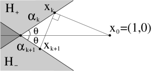
Figure 7.1. Illustration of example in Subsection 7.1.

For our modified problem, the iterates $x_{i}$ would lie on the boundary of either $H_{+}$ or $H_{-}$. For the iterate $x_{k}$, let $\alpha_{k}$ be the distance $\|x_{k}-(0,0)\|$. This is marked on Figure 7.1. The cosine rule gives us the following equations.

$$\|x_{k}-x_{k+1}\|^{2} = \alpha_{k}^{2}+\alpha_{k+1}^{2}-2\alpha_{k}\alpha_{k+1}\cos 2\theta$$ (7.2a)

$$\|x_{0}-x_{k}\|^{2} = \alpha_{k}^{2}+1-2\alpha_{k}\cos\theta$$ (7.2b)

$$\|x_{0}-x_{k+1}\|^{2} = \alpha_{k+1}^{2}+1-2\alpha_{k+1}\cos\theta.$$ (7.2c)

Pythagoras’s theorem gives us $\|x_{k}-x_{k+1}\|^{2}+\|x_{0}-x_{k}\|^{2}=\|x_{0}-x_{k+1}\|^{2}$. Together with the above equations, we have

$$\alpha_{k}^{2}-2\alpha_{k}\alpha_{k+1}\cos 2\theta-2\alpha_{k}\cos\theta = -2\alpha_{k+1}\cos\theta$$

$$\alpha_{k+1}[\cos\theta-\alpha_{k}\cos 2\theta] = -\alpha_{k}^{2}+\alpha_{k}\cos\theta$$

$$\alpha_{k+1} = \alpha_{k}\frac{\cos\theta-\alpha_{k}}{\cos\theta-\alpha_{k}\cos 2\theta}$$

$$= \alpha_{k}\left(1-\alpha_{k}\frac{1-\cos 2\theta}{\cos\theta-\alpha_{k}\cos 2\theta}\right).$$

Since $\{\alpha_{k}\}$ is a strictly decreasing positive sequence which converges to zero, we have $\alpha_{k}\geq\alpha_{k}(1-\alpha_{k}\gamma)$ for all $k$ large enough, where $\gamma=\frac{1-\cos 2\theta}{2\cos\theta}$. By Lemma 7.1, the convergence of $\{\|x_{k}-P_{H_{+}\cap H_{-}}(x_{0})\|\}$ to zero is at best $O(1/k)$.

Let $f_{k}=\|x_{0}-x_{k}\|^{2}$. To see the rate of how $f_{k}$ converges to $1$, we note from (7.2b) that $1-f_{k}=2\alpha_{k}\cos\theta-\alpha_{k}^{2}$. Then the convergence rate of $f_{k}$ to $1$ is of $\Theta(1/k)$.

7.2. The case of no linear metric inequality

Let $p\geq 1$ be some parameter. Consider the problem of projecting the point $(1,0)\in\mathbb{R}^{2}$ onto the intersection of the sets $C_{+}\cap C_{-}$, where

$$C_{\pm}=\{(u,v)\in\mathbb{R}^{2}:\pm v\geq|u|^{p}\}.$$

The diagram for this problem is similar to that of the one in Subsection 7.1. The linear metric inequality is not satisfied in this case. It is clear that the projection of $(1,0)$ onto $C_{+}\cap C_{-}$ is $(0,0)$. We try to show that the parameter $p$ can be made arbitrarily large, so that the convergence of the iterates $x_{k}$ to $\mathbf{0}=(0,0)$ is arbitrarily slow. We let $x_{k}=(u_{k},v_{k})$.

Proposition 7.2.

The iterates $x_{k}$ satisfy

$$x_{k}\notin\mbox{\rm int}(C_{+})\cup\mbox{\rm int}(C_{-}).$$ (7.3)

Proof.

This is easily seen to be true for $k=1$. We now prove that (7.3) holds for all $k$ by induction. Without loss of generality, suppose that for iterate $x_{k}$, its second coordinate $v_{k}$ is positive. The next iterate $x_{k+1}$ is the intersection of the line passing through $x_{k}$ perpendicular to $x_{0}-x_{k}$ and a supporting hyperplane of $C_{-}$. It is therefore clear that $x_{k+1}\notin\mbox{\rm int}(C_{-})$. We also see that $u_{k+1}<u_{i}$. From the convexity of $C_{+}$, if a point $x=(u,v)$ is such that $v>0$, $u<u_{1}$ and $x\notin\mbox{\rm int}(C_{+})$, then $\angle x_{0}x\mathbf{0}>\pi/2$. Given that $\angle x_{0}x_{k}\mathbf{0}>\pi/2$ and $x_{k}\notin\mbox{\rm int}(C_{+})$, we have $x_{k+1}\notin\mbox{\rm int}(C_{+})$ as well. ∎

Next, we bound the rate of decrease of $u_{k}$.

Proposition 7.3.

Continuing the discussion in this subsection, we have $u_{k+1}\geq u_{k}\left(1-\frac{2u_{k}^{2p-1}}{1-u_{k}+u_{k}^{2p-1}}\right)$.

Proof.

We assume without loss of generality that $x_{k}=(u_{k},v_{k})$ is such that $v_{k}>0$. By Proposition 7.2, we have $v_{k}\leq u_{k}^{p}$.

Consider the point $\bar{x}_{k+1}$ defined by the intersection of the line through $x_{k}$ perpendicular to $x_{k}-x_{0}$ and the line passing through $\mathbf{0}$ and $(u_{k},-u_{k}^{p})$. One can use geometrical arguments to see that $u_{k+1}\geq\bar{u}_{k+1}$, where $u_{k+1}$ is the first coordinate of $x_{k+1}$ and $\bar{u}_{k+1}$ is the first coordinate of $\bar{x}_{k+1}$. We now bound $\bar{u}_{k+1}$ from below.

The point $\bar{x}_{k+1}$ is of the form $\lambda(u_{k},-u_{k}^{p})$. From $[x_{k}-x_{0}]\perp[x_{k}-\bar{x}_{k+1}]$, we have

$$\langle(u_{k}-1,u_{k}^{p}-0),(u_{k}-\lambda u_{k},u_{k}^{p}+\lambda u_{k}^{p})\rangle = 0$$

$$\lambda u_{k}(1-u_{k})+\lambda u_{k}^{2p}+(u_{k}-1)u_{k}+u_{k}^{2p} = 0$$

$$\lambda(1-u_{k}+u_{k}^{2p-1}) = 1-u_{k}-u_{k}^{2p-1}.$$

This gives

$$u_{k+1}\geq\bar{u}_{k+1}=\lambda u_{k}=u_{k}\frac{1-u_{k}-u_{k}^{2p-1}}{1-u_{k}+u_{k}^{2p-1}}=u_{k}\left(1-\frac{2u_{k}^{2p-1}}{1-u_{k}+u_{k}^{2p-1}}\right),$$

which ends our proof. ∎

We now make an estimate of how $\|x_{k}-x_{0}\|^{2}$ converges to the optimal objective value of $1$ by analyzing $1-\|x_{k}-x_{0}\|^{2}$. We have

$$(1-u_{k})^{2}\leq\|x_{k}-x_{0}\|^{2}\leq(1-u_{k})^{2}+u_{k}^{2p}$$

$$\Rightarrow 1-(1-u_{k})^{2}-u_{k}^{2p}\leq 1-\|x_{k}-x_{0}\|^{2}\leq 1-(1-u_{k})^{2}$$

$$\Rightarrow 2u_{k}-u_{k}^{2}-u_{k}^{2p}\leq 1-\|x_{k}-x_{0}\|^{2}\leq 2u_{k}-u_{k}^{2}.$$

This means that $\{1-\|x_{k}-x_{0}\|^{2}\}$ converges to zero at the same rate $\{2u_{k}\}$ converges to zero. By Lemma 7.1 and Proposition 7.3, the convergence of $\{u_{k}\}$ to zero is seen to be at best $(\frac{1}{{}^{2p-1}\sqrt{k}})$. This means that as we make $p$ arbitrarily large, the convergence of Haugazeau’s algorithm can be arbitrarily slow in the absence of the linear metric inequality. It appears that enforcing the condition

$$C_{+}\cap C_{-}\subset\{x:\langle x_{0}-x_{k},x-x_{k}\rangle\leq 0\}$$

makes Haugazeau’s algorithm perform slower than the subgradient algorithm.

References

- [Bau96] H.H. Bauschke, Projection algorithms and monotone operators, Ph.D. thesis, Simon Fraser University, 1996.
- [BB96] H.H. Bauschke and J.M. Borwein, On projection algorithms for solving convex feasibility problems, SIAM Rev. 38 (1996), 367–426.
- [BC11] H.H. Bauschke and P.L. Combettes, Convex analysis and monotone operator theory in Hilbert spaces, Springer, 2011.
- [BD85] J.P. Boyle and R.L. Dykstra, A method for finding projections onto the intersection of convex sets in Hilbert spaces, Advances in Order Restricted Statistical Inference, Lecture notes in Statistics, Springer, New York, 1985, pp. 28–47.
- [BR09] E.G. Birgin and M. Raydan, Dykstra’s algorithm and robust stopping criteria, Encyclopedia of Optimization (C. A. Floudas and P. M. Pardalos, eds.), Springer, US, 2 ed., 2009, pp. 828–833.
- [BT09] A. Beck and M. Teboulle, A fast iterative shrinkage-thresholding algorithm for linear inverse problems, SIAM J. Imaging Sciences 2 (2009), no. 1, 183–202.
- [BZ05] J.M. Borwein and Q.J. Zhu, Techniques of variational analysis, Springer, NY, 2005, CMS Books in Mathematics.
- [Deu01] F. Deutsch, Best approximation in inner product spaces, Springer, 2001, CMS Books in Mathematics.
- [DH94] F. Deutsch and H. Hundal, The rate of convergence of Dykstra’s cyclic projections algorithm: the polyhedral case, Numer. Funct. Anal. Optimiz. 15 (1994), no. 5-6, 536–565.
- [DH06a] by same author, The rate of convergence for the cyclic projections algorithm I: Angles between convex sets, J. Approx. Theory 142 (2006), 36–55.
- [DH06b] by same author, The rate of convergence for the cyclic projections algorithm II: Norms of nonlinear operators, J. Approx. Theory 142 (2006), 56–82.
- [DH08] by same author, The rate of convergence for the cyclic projections algorithm III: Regularity of convex sets, J. Approx. Theory 155 (2008), 155–184.
- [Dyk83] R.L. Dykstra, An algorithm for restricted least-squares regression, J. Amer. Statist. Assoc. 78 (1983), 837–842.
- [ER11] R. Escalante and M. Raydan, Alternating projection methods, SIAM, 2011.
- [GI83] D. Goldfarb and A. Idnani, A numerically stable dual method for solving strictly convex quadratic programs, Math. Programming 27 (1983), 1–33.
- [Han88] S.P. Han, A successive projection method, Math. Programming 40 (1988), 1–14.
- [Hau68] Y. Haugazeau, Sur les inéquations variationnelles et la minimisation de fonctionenelles convexes, Ph.D. thesis, Université de Paris, 1968.
- [HC08] G.T. Herman and W. Chen, A fast algorithm for solving a linear feasibility problem with application to intensity-modulated radiation therapy, Linear Algebra Appl. 428 (2008), 1207–1217.
- [JN11a] A. Juditsky and A. Nemirovski, First-order methods for nonsmooth convex large-scale optimization, I: General purpose methods, Optimization for Machine Learning (S. Sra, S. Nowozin, and S.J. Wright, eds.), MIT Press, 2011, pp. 1–28.
- [JN11b] by same author, First order methods for nonsmooth convex large-scale optimization, II: Utilizing problem’s structure, Optimization for Machine Learning (S. Sra, S. Nowozin, and S.J. Wright, eds.), MIT Press, 2011, pp. 29–63.
- [Kru04] A.Y. Kruger, Weak stationarity: Eliminating the gap between necessary and sufficient conditions, Optimization 53 (2004), 147–164.
- [Kru06] by same author, About regularity of collections of sets, Set-Valued Anal. 14 (2006), 187–206.
- [Ned11] A. Nedić, Random algorithms for convex minimization problems, Math Program. Ser. B 225 (2011), 225–253.
- [Nes83] Y. Nesterov, A method for solving a convex programming problem with rate of convergence , Soviet Math. Doklady 269 (1983), no. 3, 543–547, (in Russian).
- [Nes84] by same author, Minimization methods for nonsmooth convex and quasiconvex functions, Ekonomika i Mat. Metody 11 (1984), no. 3, 519–531, (in Russian; translated as MatEcon.).
- [Nes89] by same author, Efficient methods in nonlinear programming, Radio i Sviaz, Moscow, 1989.
- [Nes04] by same author, Introductory lectures on convex optimization, Kluwer, 2004.
- [NY83] A. S. Nemirovski and D. B. Yudin, Problem complexity and method efficiency in optimization, Wiley Intersciences, 1983.
- [Pan15] C.H.J. Pang, Set intersection problems: Supporting hyperplanes and quadratic programming, Math. Program. Ser. A 149 (2015), 329–359.
- [WB15] M. Wang and D.P. Bertsekas, Incremental constraint projection methods for variational inequalities, Math. Program. Ser. A 150 (2015), 321–363.
- [Xu00] Shusheng Xu, Estimation of the convergence rate of Dykstra’s cyclic projections algorithm in polyhedral case, Acta Mathematicae Applicatae Sinica 16 (2000), no. 2, 217–220.