Trigger detection for adaptive scientific workflows using percentile sampling

Abstract

Increasing complexity of both scientific simulations and high performance computing system architectures are driving the need for adaptive workflows, in which the composition and execution of computational and data manipulation steps dynamically depend on the evolutionary state of the simulation itself. Consider for example, the frequency of data storage. Critical phases of the simulation should be captured with high frequency and with high fidelity for post-analysis, however we cannot afford to retain the same frequency for the full simulation due to the high cost of data movement. We can instead look for triggers, indicators that the simulation will be entering a critical phase, and adapt the workflow accordingly.

In this paper, we present a methodology for detecting triggers and demonstrate its use in the context of direct numerical simulations of turbulent combustion using S3D. We show that chemical explosive mode analysis (CEMA) can be used to devise a noise-tolerant indicator for rapid increase in heat release. However, exhaustive computation of CEMA values dominates the total simulation, thus is prohibitively expensive. To overcome this computational bottleneck, we propose a quantile sampling approach. Our sampling based algorithm comes with provable error/confidence bounds, as a function of the number of samples. Most importantly, the number of samples is independent of the problem size, thus our proposed sampling algorithm offers perfect scalability. Our experiments on homogeneous charge compression ignition (HCCI) and reactivity controlled compression ignition (RCCI) simulations show that the proposed method can detect rapid increases in heat release, and its computational overhead is negligible. Our results will be used to make dynamic workflow decisions regarding data storage and mesh resolution in future combustion simulations. The proposed sampling-based framework is generalizable and we detail how it could be applied to a broad class of scientific simulation workflows.

Keywords: Sublinear algorithms; quantile sampling; in situ data analysis; chemical explosive mode analysis (CEMA); S3D; adaptive workflow; judicious I/O;

1 Introduction

Steady improvements in computing resources enable ever more enhanced scientific simulations, however Input/Output (I/O) constraints are impeding their impact. Historically, scientific computing workflows have been defined by three independent stages (see Fig. 1(a)): 1) a pre-processing stage comprising initialization and set up (for example mesh generation, or initial small-scale test runs); 2) the scientific computation itself (in which data is periodically saved to disk at a prescribed frequency); and 3) post-processing and analysis of data for scientific insights. With improved computing resources scientists are increasing the temporal resolution of their simulations. However, as computational power continues to outpace I/O capabilities, the gap between time steps saved to disk keeps increasing. This compromise in the fidelity of the data being saved to disk makes it impossible to track features with timescales smaller than that of I/O frequency. Moreover, this situation is projected to worsen as we look ahead to future architectures with improvements in computational power continuing to significantly outpace I/O capabilities [26, 2], see Tab. 1.

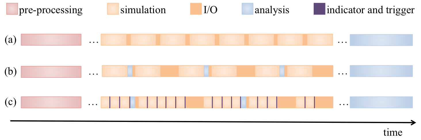
Fig. 1: (a) An illustration of a traditional workflow made up of 3 stages: 1) pre-procesing, 2) scientific computation and I/O at a prescribed rate, 3) analysis as a post-process. (b) Computational capabilities are outpacing I/O on future architectures, causing a change in workflows as some portion of the analysis moves in situ. Most current day workflows remain static, with the frequency of I/O and analysis being prescribed upfront by the scientists. (c) This paper introduces the use of indicators and triggers to support adaptive workflows. The indicator and trigger are lightweight functions evaluated at a high frequency to make dynamic data-driven control-flow decisions.

Consequently, we are seeing a paradigm shift away from the use of prescribed I/O frequencies and post-process-centric data analysis, towards a more flexible concurrent paradigm in which raw simulation data is processed in situ as it is computed, see Fig. 1 (b). In spite of the paradigm shift, concurrent processing does not provide a complete solution, as it requires all analysis questions be posed a priori. This is not always possible as scientists often analyze their data in an interactive and exploratory fashion. One potential solution, is to store data judiciously for only the time segments that will merit further analysis. However, the problem with this approach is that the computation required to automatically and adaptively make decisions regarding the workflow (e.g,. I/O and/or in situ data analysis frequencies) based on simulation state can be prohibitively expensive in their own right. Therefore, we argue that one of the more pressing fundamental research challenges is the need for efficient, adaptive, data-driven control-flow mechanisms for extreme-scale scientific simulation workflows, which is the primary goal of this work.

Table 1: Expected exascale architecture parameters for the design of two “swim lanes” of very different design choices [26, 2]. Note the drastic difference between expected improvements in I/O and compute capacities in both swim lanes.

System Parameter	2011	2018		Factor Change
System Peak	2 Pf/s	1 Ef/s		500
Power	6 MW	$\leq 20$ MW		3
System Memory	0.3 PB	32-64 PB		100-200
Total Concurrency	225K	1B$\times$ 10	1B $\times$ 100	40000-400000
Node Performance	125 GF	1TF	10 TF	8-80
Node Concurrency	12	1000	10000	83-830
Network Bandwidth	1.5 GB/s	100 GB/s	1000 GB/s	66-660
System Size (nodes)	18700	1000000	100000	50-500
I/O Capacity	15 PB	30-100 PB		20-67
I/O Bandwidth	0.2 TB/s	20-60 TB/s		10-30

Here we introduce a methodology that is broadly applicable, yet can be specialized to provide confidence guarantees for application-specific simulations and underlying phenomena. Our methodology comprises three steps:

1. Identify a noise-resistant indicator that can be used to track changes in simulation state.

2. Devise a trigger which specifies that a property of the indicator has been met.

3. Design efficient and scalable algorithms to compute indicators and triggers.

To make decisions in a data-driven fashion, a user-defined indicator function must be computed and measured in situ at a relatively regular and high-frequency. Along with the indicator, the application scientist defines an associated trigger, a function that returns a boolean value indicating that the indicator has met some property, for example a threshold value. Together, indicators and triggers define data-driven control-flow mechanisms within a scientific workflow, see Fig. 1(c). While this methodology is very intuitive and conceptually quite simple, the challenges lie in defining indicators and triggers that capture the appropriate scientific information while remaining cost efficient in terms of runtime, memory footprint, and I/O requirements so that they can be deployed at the high frequency that is required.

In this article we demonstrate how recent advances in sublinear algorithms [11, 20, 21] can be used to create efficient indicators and triggers to enable data-driven control-flow mechanisms, even in those cases where standard implementations of the indicator and trigger would be significantly too expensive. Sublinear algorithms are designed to estimate properties of a function over a massive discrete domain while 1) accessing only a tiny fraction of the domain, and 2) quantifying the error or uncertainty due to using only a sample of the data. Sublinear indicators and triggers operate on a sample whose size is dependent on the accuracy of the desired result, rather than the input size. Consequently, sublinear indicators and triggers can be deployed with high confidence to make workflow decisions in extreme-scale simulations. Sublinear algorithms have their limitations; in particular, they are not amenable for those control-flow decisions that are based on anomaly detection. However, they are well suited to control-flow decisions regarding general trends in data, e.g., based on quantile plots of trends of computationally expensive quantities of interest.

While our proposed approach is general, the first two steps can be made application dependent, leveraging some knowledge of the underlying physics. In this paper we demonstrate our approach applied to dynamic workflow decisions in the context of direct numerical simulations of turbulent combustion using S3D [8]. In this use case, workflow decisions regarding both grid resolution and I/O frequency can be made based on the detection of a rapid increase in heat release. This means our indicator should be a precursor to heat release, and not the heat release itself. What precedes the heat release? (see Fig. 3.) Recent studies have shown that chemical explosive mode analysis (CEMA) is a good lead indicator of heat release events [17, 25], and in this paper we show that CEMA can be used to devise a noise-tolerant indicator function and trigger. CEMA is a point-wise metric computed at each grid point. Our analysis of the distribution of CEMA values shows that the range of CEMA values covered by the top percentiles, compared to the full range of CEMA values, shrinks right before heat release and then expands afterwards. This change in distribution of quantiles is illustrated in Fig. 4 and provides the basis for our indicator and trigger.

Now that we have an intuition for what can be a good lead indicator for heat release, the next step is to devise an indicator function and associated trigger that quantify the shrinking/expansion of the portion of top quantiles of CEMA values over the full range. The challenge here is the noise tolerance. While the range of the CEMA values is defined by the minimum and the maximum, these values are, by definition, outliers of the distribution, and thus their adoption will lead to noise-sensitive triggers. Instead we use the quantiles of the distribution, which remain stable among instances of the same distribution. For instance, we can replace the minimum with the 1-percentile and the maximum with the 98-percentile, still capturing the concept of range, but yielding a much more noise-tolerant trigger, as supported by experimental results (see §4).

The final step is to design efficient and scalable algorithms for the indicators and triggers we have devised. Our experiments show that our CEMA-based indicators and triggers work well in practice, however, exhaustive computation of CEMA values can dominate the total simulation computation time and are thus prohibitively expensive. To overcome this computational bottleneck, we propose a sampling approach to estimate the quantiles. Our sampling based algorithm comes with provable error/confidence bounds that are only a function of the number of samples. With only 48K samples, the error will be less than %1 with confidence %99.9, which in large-scale simulation runs leads to only a few samples per processor. Most importantly, the number of samples is independent of the problem size, thus our proposed sampling algorithm offers perfect scalability. Our experiments on homogeneous charge compression ignition (HCCI) and reactivity controlled compression ignition (RCCI) simulations show that the proposed method can detect heat release, with negligible computational overhead. Moreover our results will be used to make dynamic workflow decisions regarding data storage and mesh resolution in future combustion simulations.

The rest of the paper is organized as follows. §2 provides the background for our work; we first review the need for and the state of adaptive workflows. Then we overview the mathematically rich field of sublinear algorithms and describe how this field can be instrumental in designing indicators and triggers for adaptive workflows. We conclude §2 with motivation of the combustion use case that is used throughout our paper. §3 discusses the process of identifying a noise-resistant indicator and trigger for phase change in a simulation, and includes physics intuitions for how and why CEMA can be used to construct an indicator for heat release for our combustion use case. In §4 we demonstrate how to compute the indicator and trigger efficiently using a sublinear approach and we put all the pieces together in §5 to demonstrate our technique on a full scale simulation. Finally, we conclude with §6.

2 Background

We begin this section by reviewing recent work in enabling complex scientific computing workflows. We then provide an overview of sublinear algorithms and discuss how these mathematical techniques can be deployed to make data driven decisions in situ. We conclude this section with a brief overview of our combustion use case.

2.1 Adaptive data-driven workflows and concurrent analysis frameworks

As we move to next generation architectures, scientists are moving away from traditional workflows in which the simulation state is saved at prescribed frequencies for post-processing analysis. There are a number of concurrent analysis frameworks available, wherein raw simulation output is processed as it is computed, decoupling the analysis from I/O. Both in situ [29, 7, 10] and in transit [28, 1, 4] processing are based on performing analyses as the simulation is running, storing only the results, which are typically several orders of magnitude smaller than the raw data. This reduction mitigates the effects of limited disk bandwidth and capacity. Operations sharing primary resources of the simulation are considered in situ, while in transit processing involves asynchronous data transfers to secondary resources.

Concurrent analyses are often performed at frequencies that are prescribed by the scientists a priori. For those analyses that are not too expensive – in terms of runtime (with respect to a simulation time step), memory footprint, and output size – the prescription of frequencies is a viable approach. However, for those analyses that are too expensive, prescribed frequencies will not suffice because the scientific phenomenon that is being simulated typically does not behave linearly (e.g., combustion, climate, astrophysics). When scientists choose a prescribed I/O or analysis frequency that is frequent enough to capture the science of interest, the costs incurred are too great, while a prescribed frequency that is cost-effective and less frequent may miss the underlying scientific effects that simulation is intended to capture. An alternative approach would be to perform expensive analyses and I/O in an adaptive fashion, driven by the data itself. In  [19, 18], such techniques have been developed based on entropy of information in the data, and building piecewise-linear fits of quantities of interest. These approaches fit within the methodology proposed here and are domain-agnostic. In this work we present a strategy that can leverage the scientists’ physics intuitions, even when the in situ analyses that captures those intuitions would otherwise be too expensive to compute.

2.2 Sublinear algorithms

A recent development in theoretical computer science and mathematics is the study of sublinear algorithms, which aim to understand global features of a data set while using limited resources. Often enough, we do not need to look at the entire data to determine some of its important features. The field of sublinear algorithms [11, 20, 21] makes precise the settings when this is possible and combines discrete math and algorithmic techniques with statistical tools to quantify error and give trade-offs with sample sizes. This confidence measure is necessary for adoption of such techniques by the scientific computing community, whose scientific results can be used to make high-impact decisions.

Formally, given a function, $f:D\rightarrow R$, we assume for any $x\in D$, we can query $f(x)$. For example, in S3D simulations we have $D=[n]^{3}$ as a structured grid, and $R=\mathbb{R}$ can be the temperature values. If $D=[n]$ and $R=\{0,1\}$, then $f$ represents an $n$-bit binary string. If $R=\{A,T,G,C\}$, $f$ could represent a DNA segment. If $D=[n]^{2}$, the function could represent a matrix (or a graph). Note $D$ can also be an unstructured grid, modeled as a graph. Similarly, almost any data analysis input can be cast as a collection of functions over a discrete or discretized domain.

We are interested in some specific property of $f$, which is phrased as a yes/no question. For instance, in a jet simulation we can ask if there exists a high-temperature region spanning the $x$-axis of the grid. How can we determine if $f$ satisfies property ${\cal P}$ without querying all of $f$? It is impossible to give an exact answer without knowledge of $f$. To formalize what can be inferred by querying $o(|D|)$ values of $f$, we use a notion of the distance to ${\cal P}$ . Every function $f$ has a distance to ${\cal P}$, denoted $\varepsilon_{f}$, where $\varepsilon_{f}=0$ iff $f$ satisfied ${\cal P}$. To provide an exact answer to questions regarding ${\cal P}$, we determine whether $\varepsilon_{f}=0$ or $\varepsilon_{f}\neq 0$. However, approximate answers can be given by choosing some error parameter $\varepsilon>0$ and then determining whether we can distinguish $\varepsilon_{f}=0$ from $\varepsilon_{f}>\varepsilon$. The theory of sublinear algorithms shows whether the latter question can be resolved by an algorithm that samples $o(|D|)$ function values.

For a sublinear algorithm, there are usually three parameters of interest: the number of samples $t$, the error $\varepsilon$, and the confidence $\delta$. As described earlier, the error is expressed as the distance to ${\cal P}$. Analysis shows that for a given $t$, we can estimate the answer within error $\varepsilon$ with a confidence of $>1-\delta$. Conversely, given $\varepsilon,\delta$, we can compute the number of samples required.

Although at a high level, any question that can be framed in terms of determining global properties of a large domain is subject to a sublinear analysis, surprisingly, the origins of this field have nothing to do with “big data” or computational challenges in data analysis. The birth of sublinear algorithms is in computational complexity theory [22]. Hence, practical performances of these methods on real applications have not been fully investigated. Recent work by some of the authors showcase the potential of sampling algorithms in graph analysis [23, 24, 16, 14, 13, 3], and the generation of application-independent generation of colormaps [27].

2.3 Potential of sublinear algorithms in enabling adaptive workflows

The construction of a scalable and performant indicator function comprises a number of technical challenges. First, algorithms will be sharing compute resources with the simulation, which poses constraints on the algorithmic choices. In particular, memory is expected to be a bottleneck in exascale computers and beyond (see Tab. 1), and thus we may have to work with data structures of the application, and not be able to build auxiliary data structures that will improve the performance of our algorithms. Secondly, the data layout will be dictated by the simulation, locally at the node level and globally at the system level. This layout will not necessarily be favorable for our algorithms, yet pre-processing to move the data will be infeasible at large scales. Thirdly, computation of the indicator needs to be fast, so that it does not slow down the simulation computation. For instance, our analysis for judicious I/O cannot take more time than the I/O itself.

We expect sampling-based algorithms, especially sublinear algorithms, to play an important role in the design of indicator functions at the exascale era and beyond. First, the small number of samples grant runtime efficiency, which enable working concurrently with the simulation, with negligible effect on runtime. The error/confidence bounds quantify the compromise in accuracy compared to full analysis. Moreover, for most problems, the number of samples required only depend on error/confidence bounds, which lead to perfect scalability of these algorithms for extreme problem sizes. The memory requirements of sublinear algorithms are also small, and typically only in the order of the samples. In some cases, additional data structures may be necessary to enable random sampling, but even such structures are not memory-intensive.

We claim that sublinear algorithms can play a critical role for in situ analysis. With this paper, we will showcase one application of sublinear algorithms, and we hope that our success will draw attention to this field with high potential.

2.4 Combustion use case

Throughout this paper we demonstrate our approach applied to a combustion use case, using S3D [8], a direct numerical simulation (DNS) of combustion in turbulence. The combustion simulations in our use case pertain to a class of internal combustion (IC) engine concept, called premixed-charge compression ignition (PCCI). The central idea is that the air-fuel mixture is allowed to ignite on its own, as opposed to being forced to ignite through a spark, as is done in conventional spark-ignited (SI) engines. This results in substantial improvements in fuel efficiency. However, one of the roadblocks to this technology is that the ignition is difficult to control. In particular, it is difficult to predict the precise moment of ignition, which is important for such an engine to be practical. It is undesirable to have simultaneous ignition of the entire mixture, or even a large fraction of the mixture, which would result in knocking, damaging the engine.

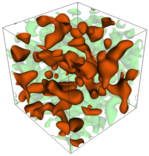
Fig. 2: In a Homogenous Compression Charge Ignition simulation many small heat kernels slowly develop prior to auto-ignition. In this image, regions of high heat kernels are shown in orange and regions of high vorticity are shown in green.

Within the broad framework of PCCI, several ideas have been proposed to alleviate the difficulty noted above. All of them seek to control the ignition process by staggering it in time, i.e. different parcels of the air-fuel mixture ignite at different times, so that the overall heat release is delocalized in time. This is done typically by stratifying the mixture, i.e. mixture properties are varied spatially in such a way that the desired heat release profile is obtained. Here, we are interested in two specific techniques called homogeneous-charge compression ignition (HCCI) [5] and reactivity-controlled compression ignition (RCCI) [15, 6]. In both cases, heat release starts out in the form of small kernels at arbitrary locations in the simulation domain, see Fig. 2. Eventually, multiple kernels ignite as the overall heat release reaches a global maximum and subsequently declines. Since these simulations are computationally and storage-intensive, we want to run the simulation at a coarser grid resolution and save data less frequently during the early build-up phase. When the heat release events occur, we want to run the simulation at the finest grid granularity possible, and store the data as frequently as possible. Therefore, it is imperative to be able to predict the start of the heat release event using an indicator and trigger that serve to inform the application to adjust its grid resolution and I/O frequency accordingly, see Fig. 3.

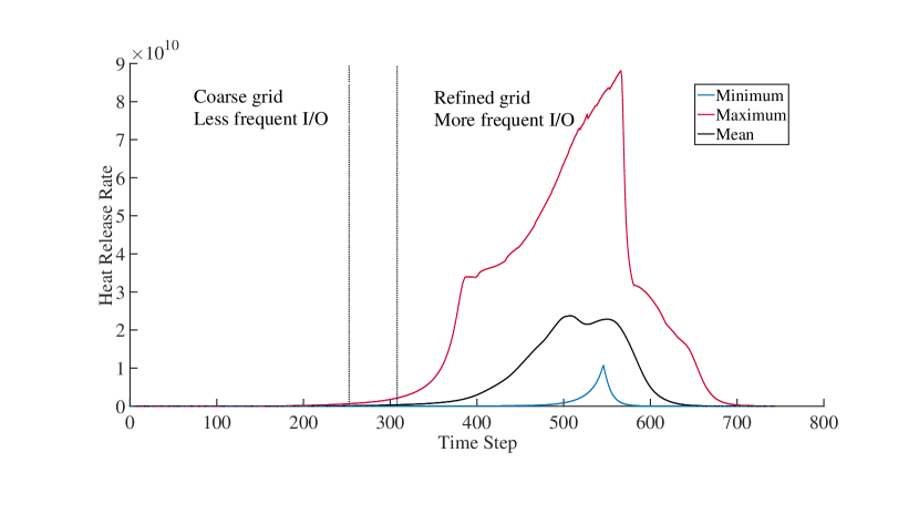
Fig. 3: The minimum (blue), maximum (red) and mean (black) heat release values for each time step in the simulation. Early in the simulation, we want to run at a coarser grid resolution and save data less frequently. When heat release events occur, we want to run the simulation at the finest granularity, and save the data as frequently as possible. The vertical dotted lines in this figure define a range of time steps within which we would like to make this workflow transition (as identified by a domain expert).

3 Designing a Noise-Resistant Indicator and Trigger

While general-purpose indicators could be computed (e.g. entropy of a quantity of interest), we argue that application domain-specific indicators in many cases will best capture the phenomena of interest. In this section we describe the design of an indicator and trigger for heat release for our combustion use case. To provide context, we begin by discussing the intuitions that informed our design.

3.1 Chemical Explosive Mode Analysis

One of the most reliable techniques to predict incipient heat release is the chemical explosive mode analysis (CEMA). CEMA is a pointwise computational technique described in detail by Lu et al. [17] and Shan et al. [25]. A brief description is provided here for reference. The conservation equations for reacting species can be written as

$$\frac{D\mathbf{y}}{Dt}=\mathbf{g(y)}\equiv\mathbf{\omega(y)}+\mathbf{s(y)}$$

The vector $\mathbf{y}$ in CEMA represents temperature and reacting species mass fractions, $\mathbf{\omega}$ is the reaction source term and $\mathbf{s}$ is the mixing term. The Jacobian of the right hand side can be written as

$$\mathbf{J_{g}}=\frac{\partial\mathbf{g(y)}}{\partial\mathbf{y}}=\mathbf{J_{\omega}}+\mathbf{J_{s}},\;\;{\mathrm{w}here}\;\;\mathbf{J_{\omega}}=\frac{\partial\mathbf{\omega(y)}}{\partial\mathbf{y}}\;\;{\mathrm{a}nd}\;\;\mathbf{J_{s}}=\frac{\partial\mathbf{s(y)}}{\partial\mathbf{y}}.$$

The chemical Jacobian, $\mathbf{J_{\omega}}$ can be used to infer chemical properties of the mixture. This is done using an eigen-decomposition of the Jacobian. If the eigenvalues of the Jacobian corresponding to the non-conservative modes are arranged in descending order of the real part, $\lambda_{e}$ is defined as the first eigenvalue and $\lambda_{i}$ are the remaining eigenvalues. The eigenmode associated with $\lambda_{e}$ is defined as a chemical explosive mode (CEM) if

$$\textrm{Re}(\lambda_{e})>0,\;\;{\mathrm{f}or}\;\;\lambda_{e}=\mathbf{b_{e}J_{\omega}a_{e}},$$ (1)

where $\mathbf{b_{e}}$ and $\mathbf{a_{e}}$ are the left and right eigenvectors respectively for $\lambda_{e}$. The presence of a CEM indicates the propensity of a mixture to ignite. CEMA is a pointwise metric, typically computed at every grid point in the simulation domain. The criterion defined above then indicates whether that point will undergo ignition or whether it has already undergone ignition. If it has undergone ignition, we have $Re(\lambda_{e})<0$.

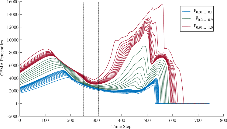
Fig. 4: In this percentile plot of CEMA values, the lowest blue curve and the highest red curve correspond to the 1 and 100 percentiles ($p_{0.01}$ and $p_{1}$), respectively. The blue curves correspond to $p_{0.01\ldots 0.1}$, the green curves to $p_{0.2\ldots 0.9}$ and the red curves to $p_{0.91\ldots 1}$. We notice that as the simulation progresses, the distance between the higher percentiles (red curves) decreases then suddenly increases. Our aim is to define a function that captures when this spread in the high percentiles occurs, as this serves as a good indicator of ignition (it falls within the user-defined window of true trigger time steps, indicated by the vertical dotted lines).

Our CEMA-based indicator is based on global trends of CEMA over time. Consider Fig. 4 which provides a summary of the trends of CEMA values across all time steps in a simulation. At timestep $t$, let ${\cal C}(t)$ be the array of CEMA values on the underlying mesh. It is convenient to think of ${\cal C}(t)\in\mathbb{R}^{N}$, where $N$ is the total number of grid points. This array is distributed among $M$ processors such that each process accesses $N/M$ points of the field. Let $\widehat{{\cal C}(t)}$ be the sorted version of ${\cal C}(t)$. For $\alpha\in(0,1]$, the $\alpha$-percentile is the entry $\widehat{{\cal C}(t)}_{\lceil\alpha N\rceil}$. More specifically, it is the value in $\widehat{{\cal C}(t)}$ that is greater than at least $\lceil\alpha N\rceil$ values in $\widehat{{\cal C}(t)}$. We denote this value by ${p}_{\alpha}(t)$.

We notice that as the simulation progresses, the distance between the higher percentiles (red curves) decreases then suddenly increases. This is illustrated in the plot by the spread in the red curves that occurs just before the dashed line (indicating ignition). What does this mean? Suppose the range of CEMA values (at time $t$) is $[x,y]$. If the distribution of CEMA values was uniform in $[x,y]$, then the $\alpha$-percentile would have value around $x+\alpha(y-x)$. Suppose the distribution was highly non-uniform, with a large fraction of small (close to $x$) values. Then, for large $\alpha$, we expect the $\alpha$-percentile to be smaller than $x+\alpha(y-x)$. Alternately, for (large) $\alpha<\beta$, in the uniform case, the difference between these percentiles is $(\beta-\alpha)(y-x)$. If many values are small, we expect this difference to be larger. Essentially, the gaps between the high percentiles become larger as more CEMA values move towards the lower end of the range.

Our empirical observation is consistent with the underlying physics. From a physical point of view, this trend in the distribution of CEMA values indicates the formation of the first ignition kernels in the fuel-air mixture. As some of these kernels become fully burnt, their CEMA values become negative. As a parcel of fluid transitions from fully unburnt to partially burnt to fully burnt, its temperature increases monotonically and the CEMA value associated with it reaches a peak value before crossing zero and attaining a negative value indicating a fully burnt state. The CEMA values for several other kernels that are in different stages of ignition, i.e. partially burnt, lie between those for unburnt (large positive) and burnt (negative) mixtures. The large range of CEMA values in partially burnt mixtures explains the range of values seen in the percentile plots as ignition is initiated in the mixture.

3.2 Designing a Noise-Resistant CEMA-Based Indicator

We introduce an indicator function, P-indicator that quantifies the distribution of the top quantiles of CEMA values over time. The P-indicator measures the ratio of the range of the top percentiles to the full range of CEMA values. Our indicator function relies on the range of CEMA values, which are defined by their minimum and maximum. However, the maximum and the minimum of a distribution, by definition, are outliers, and thus they can change drastically between instances even when the underlying distribution does not change. Hence, we avoid the maximum and minimum and replace them with high and low quantiles of the distribution.

Formally, quantiles are defined as values taken at regular intervals from the inverse of the cumulative distribution function of a random variable. For a given data set, quantiles are used to divide the data into equal sized sets after sorting, and the quantiles are the values on the boundary between consecutive subsets. A special case is dividing 100 equal groups, when we can refer to quantiles as percentiles. This paper focuses on percentiles with numbers in the $[0,1]$ range (although all techniques presented here can be generalized for any quantiles). For example, the $0.5$ percentile will refer to the median of the data set.

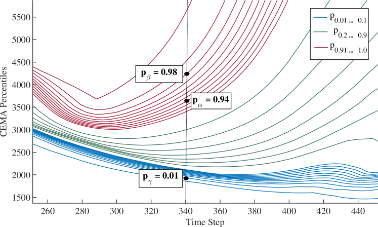
Fig. 5: $P_{\alpha,\beta,\gamma}(t)$ values evaluated at each time step. Here we illustrate $\alpha_{0}=0.94$, $\beta=0.98$ and $\gamma=0.01$ for time step 340 of a simulation.

We substitute the maximum with a high percentile, which we denote by the $\beta$-percentile where $\beta$ is typically in the range $[0.95,0.99]$ and the minimum with a low percentile, which we denote by the $\gamma$-percentile where $\gamma$ is typically in the range $[0.01,0.05]$. This substitution provides stability to our measurements, without compromising what we want to measure.

Consider the following notation: Let $A\in\mathbb{R}^{N}$, be an array in sorted order. The $\alpha$ percentile of this sorted array is exactly the entry $A_{\lceil\alpha N\rceil}$. We use ${p}_{\alpha}$ to refer to this value (i.e., ${p}_{\alpha}=A_{\lceil\alpha N\rceil}$. The $A$ array will change at each step of the simulation, and thus we will use $A(t)$ and ${p}_{\alpha}(t)$ to refer to the data on step $t$ of the simulation.

We define our indicator on a given array $A$ using 3 parameters: $\alpha$, $\beta$ and $\gamma$. As described above, we use ${p}_{\beta}(t)$ and ${p}_{\gamma}(t)$ as substitutes for the maximum and the minimum of $A(t)$ respectively, see Fig. 5. We want to detect whether the range covered by top quantiles shrinks, and $\alpha$ represents the lower end of the top quantiles. Therefore, the range of top quantiles we measure is $\left[{p}_{\alpha}(t),{p}_{\beta}(t)\right]$. In our indicator, we choose $\alpha<\beta$ (typically in the range $[0.95,0.99]$) and $\gamma$ (typically in the range $[0.01,0.05]$). We measure the spread at time $t$ by the P-indicator:

$$P_{\alpha,\beta,\gamma}(t)=\frac{{p}_{\alpha}(t)-{p}_{\gamma}(t)}{{p}_{\beta}(t)-{p}_{\gamma}(t)}.$$ (2)

In this indicator, the denominator corresponds to the full range of CEMA values, while the numerator corresponds to the range after the top quantiles are removed. When the CEMA values are uniformly distributed, $P_{\alpha,\beta,\gamma}(t)\approx(\alpha-\gamma)/(\beta-\gamma)$ $\approx\alpha/\beta$. When there is a significant shift towards lower values, $P_{\alpha,\beta,\gamma}(t)$ will become smaller.

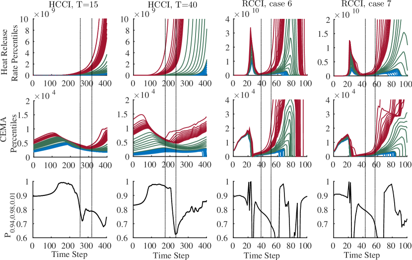
Fig. 6: Plots showing the (top row) percentiles of the heat release rate, (middle row) percentiles of CEMA, and (bottom row) the P-indicator, as indicated. In the percentile plots, the lowest blue curve and the highest red curve correspond to the 1 and 100 percentiles ($p_{0.01}$ and $p_{1}$), respectively. The blue curves correspond to $p_{0.01\ldots 0.1}$, the green curves to $p_{0.2\ldots 0.9}$ and the red curves to $p_{0.91\ldots 1}$. The P-indicator shown is evaluated for $\alpha_{0}=0.94$, $\beta=0.98$ and $\gamma=0.01$. The vertical dotted lines crossing the images indicate a window of acceptable “true” trigger time steps, as identified by a domain expert. For the RCCI cases, the trigger time ranges are based on the High Temperature Heat Release (HTHR), i.e., the second peak in the Heat Release Rate (HRR) profiles.

Fig. 6 illustrates percentile plots for heat release (top row) and CEMA (middle row). In the percentile plots, the lowest blue curve and the highest red curve correspond to the 1 and 100 percentiles ($p_{0.01}$ and $p_{1}$), respectively. The blue curves correspond to $p_{0.01\ldots 0.1}$, the green curves to $p_{0.2\ldots 0.9}$ and the red curves to $p_{0.91\ldots 1}$. The P-indicator evaluated using (2) for $\alpha=0.94$, $\beta=0.98$ and $\gamma=0.01$ is shown in the bottom row of Fig. 6. Results are generated for four test cases described in Tab. 2. The vertical dotted lines were identified by a domain expert who, via examination of heat release and CEMA percentile plots, visually located the time steps in the simulation where the mesh resolution and I/O frequency should be increased. We refer to these time steps as the “true” trigger time steps we wish to identify with the P-indicator and trigger functions. Note, for the RCCI cases, there are two ignition ranges. To simplify the following exposition, we focus on the second rise in the heat release rate profiles, as this is the ignition stage of interest to the scientists. However, we note that our approach is robust in identifying the first ignition stage as well.

Table 2: Four Combustion Use Cases analyzed in this study. The “true” trigger time ranges are estimated based on $95-100^{\textrm{th}}$ percentiles of the heat release rate. The computed time ranges were evaluated using our quantile sampling approach. For the RCCI cases, the trigger time ranges are based on the High Temperature Heat Release, i.e., the second peak in the Heat Release Rate profiles.

Problem	Number of	Number of	“True” Trigger	Computed
Instance	Grid Points	Species	Time Range	Trigger Time
HCCI, T=15	451,584	28	250-315	250-262
HCCI, T=40	451,584	28	175-225	213-220
RCCI, case 6	2,560K	116	38-50	28-45
RCCI, case 7	2,560K–10,240K	116	42-58	35-50

3.3 Defining a Trigger

In addition to defining a noise-resistant indicator function, we also need to define a trigger function that returns a boolean value, capturing whether a property of the indicator has been met. Looking at Fig. 6, we notice that across all experiments from Tab. 2, the P-indicator is decreasing during the true trigger time step windows. Therefore, we seek to find a value $\tau_{P}\in(0,1)$, such that $P_{\alpha,\beta,\gamma}(t)$ crosses $\tau_{P}$ from above, as the simulation time $t$ progresses.

Fig. 7 plots the trigger time steps as a function of $\tau_{P}$ for a variety of configurations of $\alpha$ and $\beta$ for the four use cases desribed in Tab. 2. The horizontal dashed lines indicate the true trigger range identified by our domain expert. We consider those values of $\tau_{P}$ that fall within the horizontal dashed lines to be viable $\tau_{P}$ values for our trigger. We find that across all use cases, there are similar viable ranges of values for $\tau_{P}$ where the predicted trigger time steps do not exhibit large variations. In Fig. 8 we provide a plot the trigger time steps as a function of $\tau_{P}$ for $P_{\alpha=0.94,\beta=0.98,\gamma=0.01}(t)$ that shows the viable range of $\tau_{P}$ is $[0.725,0.885]$.

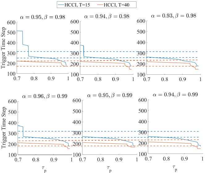
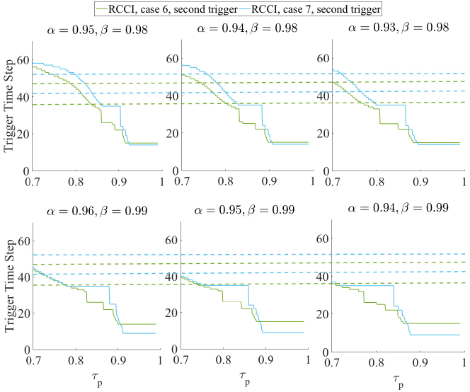
Fig. 7: This figure shows the trigger time steps as a function of $\tau_{P}$ for a variety of configurations of $\alpha$ and $\beta$ for the four use cases desribed in Tab. 2. The horizontal dashed lines indicate the true trigger range identified by our domain expert. The P-indicator is evaluated with percentiles computed using all $N$ grid points for the different use cases, as indicated.

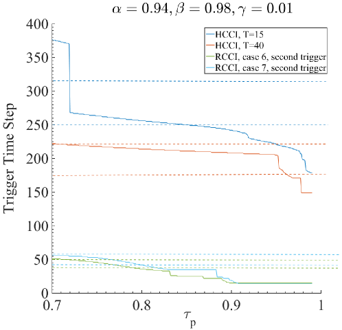
Fig. 8: This figure plots the trigger time steps as a function of $\tau_{P}$ for $P_{\alpha=0.94,\beta=0.98,\gamma=0.01}(t)$. There is a range of viable values of $\tau_{P}\in[0.725,0.885]$ that predict early stage heat release.

4 Computing Indicators and Triggers Efficiently: A Sublinear Approach

The previous section showed that a CEMA-based P-indicator and trigger are robust to noise fluctuations and act as a precursor to rapid heat release in combustion simulations. In this section we provide some details regarding its computational cost, which can be prohibitive for large-scale simulations. We then introduce an efficient method to estimate the P-indicator. Our method is based on quantile sampling and it comes with provable bounds on accuracy as a function of the number of samples. Most importantly, the required number of samples for a specified accuracy is independent of the size of the problem, hence our sampling based algorithms offers excellent scalability.

4.1 Computational Cost of CEMA

Although CEMA is useful for predicting ignition, it is expensive to compute and thus historically has not been used as a predictive measure. Computing CEMA values involves constructing a large, dense matrix at every grid point, and computing its eigendecomposition. For the use cases considered here, the time taken to compute the CEMA values scales as the time taken to compute the eigendecomposition of an $M\times M$ matrix, where $M$ is the number of species. Since the Jacobian does not have any spatial structure, the time taken for the CEMA computation step is $\textbf{O}(M^{3})$, which makes it increasingly expensive for larger chemical mechanisms. As seen in Tab. 3, for the ethanol HCCI case presented here that was simulated with $28$-species, the cost of computing the CEMA value at every grid point was approximately $5$ times the cost of one simulation time-step. The RCCI case, on the other hand included $116$-species and the cost was roughly $60$ times that of a single time step. Although it is infeasible to compute CEMA at every grid point, our indicator function is defined in terms of distribution of CEMA values, ${\cal C}(t)$, and this can be easily approximated by a sampling mechanism, that has provable guarantees on the error.

4.2 Approximating percentiles by sampling

To remind our notation, we have an array $A\in\mathbb{R}^{N}$, in sorted order. Our aim is to estimate the $\alpha$-percentile of $A$. (We use ${p}_{\alpha}$ to denote the percentiles.) Note that this is exactly the entry $A_{\lceil\alpha N\rceil}$. Here is a simple sampling procedure.

1. Sample $k$ independent, uniform indices $r_{1},r_{2},\ldots,r_{k}$ in $\{1,2,\ldots,N\}$.
   Denote by $\widehat{A}$ the sorted array $[A(r_{1}),A(r_{2}),\ldots,A(r_{k})]$.

2. Output the $\alpha$-percentile of $\widehat{A}$ as the estimate, $\widehat{{p}}_{\alpha}$.
   

In the next section, we quantitatively show that our estimation, $\widehat{{p}}_{\alpha}$, is approximately close to the the true ${p}_{\alpha}$. Such sampling arguments were also used in automatic generation of colormaps for massive data [27].

4.3 Theoretical bounds on performance

Our analysis relies on the following fundamental result by Hoeffding, which provides a concentration inequality for sums of independent random variables.

Theorem 1 (Hoeffding [12] or Theorem 1.1 in [9]).

Let $X_{1},X_{2},\dots,X_{k}$ be independent random variables with $0\leq X_{i}\leq 1$ for all $i=1,\dots,k$. Define $X=\frac{1}{k}\sum_{i=1}^{k}X_{i}$. For any positive $t$, we have

$$\Pr[|X-\hbox{\bf E}[X]|\geq t]\leq 2\exp(-2t^{2}/k).$$

Lemma 2.

Fix $\alpha$ and parameters $\delta,\varepsilon\in(0,1)$, such that $\alpha>\varepsilon$ and $\alpha+\varepsilon\leq 1$. Set $k=\lceil\frac{\log(4/\delta)}{2\varepsilon^{2}}\rceil$. Then $\widehat{{p}}_{\alpha}\in[{p}_{\alpha-\varepsilon},{p}_{\alpha+\varepsilon}]$ with probability at least $1-\delta$.

Proof.

Let $X_{i}$ be the (Bernoulli) indicator random variable for the event $r_{i}<(\alpha-\varepsilon)N$. (i.e.,$X_{i}=1$, if $r_{i}<(\alpha-\varepsilon)N$, and zero otherwise.) Note that

$$\hbox{\bf E}[X_{i}]=\Pr[X_{i}=1]=\Pr[r_{i}<(\alpha-\varepsilon)N]<\alpha-\varepsilon.$$

By linearity of expectation, $\hbox{\bf E}[\sum_{i\leq k}X_{i}]<k(\alpha-\varepsilon)$. By Hoeffding’s inequality (Thm. 1),

$$\Pr[\sum_{i\leq k}X_{i}-\hbox{\bf E}[\sum_{i\leq k}X_{i}]\geq\varepsilon k]\leq 2\exp(-2\varepsilon^{2}k).$$

The latter is at most $\delta/2$. Thus, with probability $>1-\delta/2$,

$$\sum_{i\leq k}X_{i}\leq\hbox{\bf E}[\sum_{i\leq k}X_{i}]+\varepsilon k<\alpha k.$$

In plain English, with probability at least $1-\delta/2$, the number of random indices strictly less than $(\alpha-\varepsilon)N$ is strictly less than $\alpha k$.

We repeat a similar argument with indicator random variable $Y_{i}$ for the event $r_{i}<(\alpha+\varepsilon)N$. So $\hbox{\bf E}[Y_{i}]>\alpha+\varepsilon$ and $\hbox{\bf E}[\sum_{i\leq k}Y_{i}]>k(\alpha+\varepsilon)$. By Hoeffding’s inequality,

$$\Pr[\hbox{\bf E}[\sum_{i\leq k}Y_{i}]-\sum_{i\leq k}Y_{i}>\varepsilon k]<\delta/2.$$

With probability at least $1-\delta/2$, the number of random indices at most $(\alpha+\varepsilon)N$ is strictly more than $\alpha k$.

By the union bound on probabilities, both events hold simultaneously with probability $>1-\delta$. In this situation, the $\alpha$-percentile of the sample lies between the ${p}_{\alpha-\varepsilon}$ and ${p}_{\alpha+\varepsilon}$. ∎

Table 3: Additional cost associated with computing CEMA indices at every grid point (no sub-sampling) for two chemical mechanisms. Cost is given in seconds of wall-clock time per overall simulation time step.

Fuel	Mechanism	Cost without	Cost with	Cost
	size (species)	CEMA (sec/ts)	CEMA (sec/ts)	factor
Ethanol	$28$	$0.3$	$1.5$	$5$
Primary Reference
Fuel (PRF)	$116$	$3.0$	$180.0$	$60$

It bears emphasizing that the number of samples, $k$, is independent of the problem size, $N$, and only depends on $\varepsilon,\delta$. So, the required number of samples only depends on the desired accuracy, not on the size of the data. This is the key to the scalability of our approach.

To compute the P-indicator, $P_{\alpha,\beta,\gamma}$, we just employ the procedure above to get estimates $\widehat{{p}}_{\alpha},\widehat{{p}}_{\beta},\widehat{{p}}_{\gamma}$. We can use the same samples (with only an additive increase to $k$) for all estimates, so we do not have to repeat the procedure $3$ times. That yields the approximate P-indicator, denoted by $\widehat{P}_{\alpha,\beta,\gamma}$.

Theorem 3.

Fix $\alpha,\beta,\gamma$ and parameters $\delta,\varepsilon\in(0,1)$ such that $\alpha<\beta-2\varepsilon$ and $\varepsilon<\min(\alpha,\beta,\gamma)$. Set $k=\lceil\frac{\log(12/\delta)}{2\varepsilon^{2}}\rceil$. With probability $>1-\delta$,

$$\widehat{P}_{\alpha,\beta,\gamma}\in[P_{\alpha-\varepsilon,\beta+\varepsilon,\gamma+\varepsilon},P_{\alpha+\varepsilon,\beta-\varepsilon,\gamma-\varepsilon}].$$

Proof.

Apply Lem. 2 for each of $\alpha,\beta,\gamma$ with error parameter $\delta/3$. That gives the value of $k$ as stated in the theorem. By the union bound on probabilities, all the following hold simultaneously with probability $>1-\delta$: $\widehat{{p}}_{\alpha}\in[{p}_{\alpha-\varepsilon},{p}_{\alpha+\varepsilon}]$, $\widehat{{p}}_{\beta}\in[{p}_{\beta-\varepsilon},{p}_{\beta+\varepsilon}]$, and $\widehat{{p}}_{\gamma}\in[{p}_{\gamma-\varepsilon},{p}_{\gamma+\varepsilon}]$, Hence,

$$\widehat{P}_{\alpha,\beta,\gamma}=\frac{\widehat{{p}}_{\alpha}-\widehat{{p}}_{\gamma}}{\widehat{{p}}_{\beta}-\widehat{{p}}_{\gamma}}\leq\frac{{p}_{\alpha+\varepsilon}-\widehat{{p}}_{\gamma}}{{p}_{\beta-\varepsilon}-\widehat{{p}}_{\gamma}}\leq\frac{{p}_{\alpha+\varepsilon}-{p}_{\gamma-\varepsilon}}{{p}_{\beta-\varepsilon}-{p}_{\gamma-\varepsilon}}$$

For the last inequality, observe that for fixed $x<y$, $(x-z)/(y-z)$ is a decreasing function of $z$. An analogous argument proves the lower bound for $\widehat{P}_{\alpha,\beta,\gamma}$. ∎

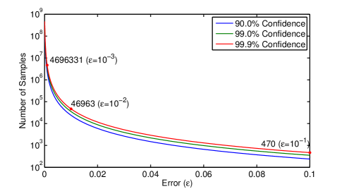
Fig. 9: The number of samples needed for different error rates and different levels of confidence. A few data points at 99.9% confidence are highlighted.

Fig. 9 shows the number of samples needed for different error and confidence rates. We show three different curves for difference confidence levels. Increasing the confidence has minimal impact on the number of samples. The number of samples is fairly low for error rates of 0.1 or 0.01, but it increases with the inverse square of the desired error. Nonetheless, the four million samples required for an error rate of $\varepsilon=.001$ at 99.9% confidence requires only tens of samples per processor at the extreme scales. In practice, $\varepsilon=.01$ at 99.9% confidence, thus 48,000 samples was enough to compute robust estimates.

4.3.1 Interpretation of the bounds

Our bounds on quantile estimations are based on which quantile we sample. That is our sampling algorithm may return the $\alpha+\varepsilon$-th quantile instead of $\alpha$-th quantile, and we can quantify this error, $\varepsilon$, as a function of the number of samples. However, it does not quantify the difference between ${{p}}_{\alpha}$ and $\widehat{{p}}_{\alpha}={{p}}_{\alpha+\varepsilon}$. Subsequently, Thm. 3 shows that the range we sample can be made arbitrarily close to the original range by increasing the number of samples, and bounds the error in the range for any given sample size. Yet, it does not bound the difference between $P_{\alpha,\beta,\gamma}$ and $\widehat{P}_{\alpha,\beta,\gamma}$, which depends on the distribution of the data. However, this is not a critical issue for our purposes, as we argue next, and empirically verify with experimental results in the next section.

The difference between $P_{\alpha,\beta,\gamma}$ and $\widehat{P}_{\alpha,\beta,\gamma}$ will be disproportional to $\varepsilon$ only when there are gaps in the distribution around one of the three parameters, $\alpha$, $\beta$, or $\gamma$. Note that these three parameters are user specified, and they are used to quantify the range of top percentiles. If the underlying distribution is such that we expect many such gaps frequently, then our metric itself will be extremely sensitive to the choice of the input parameters, even if compute the metric exactly. That is our metric should not produce vastly different results when we choose $\alpha=0.940$ or $\alpha=0.941$. However, there is still a possibility that such gaps may form, just like any other low probability event. One trick to improve robustness of our metric against such low probability events is to pick the input parameters randomly from a specified range. That is instead of specifying $\gamma$ as $0.03$ we can pick it randomly in the range $[0.02,0.04]$. By such randomness, even if there is a gap at point, $\phi$, the probability that $\phi$ is in the $[\beta-\varepsilon,\beta+\varepsilon$] range will approach to zero with increasing number of samples and thus decreasing $\varepsilon$.

However, we want to note that this is only a theoretical exercise. From a practical perspective, we have not observed any gaps in the distribution and ${{p}}_{\alpha+\varepsilon}$ is a good estimate for ${{p}}_{\alpha}$, and it gets better with more samples. For the experiments in the remainder of this paper, we have not used the randomization technique when choosing the parameters, $\gamma$, $\alpha$, and $\beta$.

4.4 Empirical evaluation of the sampling based algorithm

In this section we present our empirical evaluation of the proposed sampling techniques. Experiments in this section will focus on only the evaluation of the proposed algorithm, since we first want to verify that the proposed sampling technique accurately estimates the P-indicator. In the next section, we will put all pieces together and study how the P-indicator and the proposed technique perform together in situ as the simulation is running.

In the first set of experiments, we investigate the error in quantile ranges. For these experiments, we use 16 randomly selected instances of CEMA distributions from various HCCI and RCCI simulations. These instances are named such that the first part refers to the simulation type and case, and the last part refers to the time step. We use sampling to estimate the $\alpha=0.94$ percentile, which returns an entry from the distribution. Then we check the percentile of this entry in the full data, say $\alpha+\varepsilon$. In the first set of experiments, we focus on this difference $\varepsilon$, which we bounded in our theoretical analysis.

Fig. 10 (a) presents the results of our investigation into the error of quantile ranges for various data sets and increasing number of samples: 12,000, 24,000, and 48,000. For this figure, we ran our sampling algorithm 100 times for each instance (i.e., a data set and number of samples combination) and computed $\varepsilon$. The figure presents the average $|\varepsilon|$ for each instance. As the figure shows, sampling yields accurate estimations in all data sets, and the error drops with increasing number of samples. It becomes extremely small for 48,000 samples. Here an error of 0.001 means we will be using ${{p}}_{0.941}$ quantile instead of ${{p}}_{0.940}$. We did not find it necessary to investigate increasing the number of samples further.

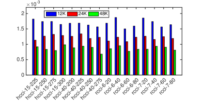
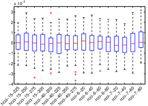
(a)Average error	(b) Distribution of errors

Fig. 10: (a) Error in the percentile sampled as the average of absolute values of 100 runs on various data sets with increasing number of samples. (b) The distribution of errors of each data set for the percentile study using 48,000 samples.

In Fig. 10 (b), we show the distribution of errors in percentiles sampled for the 100 runs of each dataset using 48,000 samples. In this plot, the central mark (red) shows the median error, while the edges of the (blue) box are the 25th and 75th percentiles. The whiskers extend to the most extreme points considered not to be outliers, and the outliers (red plus marks) are plotted individually. As this figure shows, the estimates are consistently accurate, and the results in practice are much better than those indicated by Thm. 3. According this theorem, 48,000 samples lead to an error of $\approx 0.01$ with a confidence of %99. This means in 100 experiments we expect to have 1 run for which the error is $>0.01$. However, in the 16 data sets with 100 runs each the maximum error was $0.005$, half of what the upper bound indicates. These results show that sampling enables us to sample a quantile that is consistently accurate.

In the next set of experiments, we look at how our indicator is affected by the minor errors in the quantile. More specifically, we want to see how the difference between ${{p}}_{\alpha}$ and ${{p}}_{\alpha+\varepsilon}$ affect our indicator. For those experiments, we used 16 randomly selected instances of CEMA distributions from various HCCI and RCCI simulations and computed the P-indicator exactly, and using sampling with parameters, $\gamma=0.01$ $\alpha=0.94$, and $\beta=0.98$.

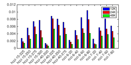
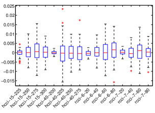
(a) Average Error	(b) Distribution of errors

Fig. 11: (a) Errors in estimation of the P-indicator for increasing number of samples. (b) The distribution of errors in estimation of the P-indicator for 48,000 samples.

While we repeated the same experiments with different parameters, we have not observed any sensitivities of our tests to the choice the parameters, hence we will present results for only this setting.

Fig. 11(a) presents results for our indicator tests for various data sets and increasing number of samples: 12,000, 24,000, and 48,000. For this figure, we ran our sampling algorithm 100 times on each data set and number of samples, and computed the difference between exact and estimated values of the P-indicator for each instance. The figure presents the average absolute error for each instance. As the figure shows, sampling produces accurate estimations in all data sets, and the error drops with increasing number of samples. The bounds on Thm. 3 does not apply in this case. but regardless, the errors are very small, and certainly sufficient to detect any trend in the distribution of the underlying values.

Fig. 11(b) shows the distribution of errors for the P-indicator test for 100 runs of each dataset using 48,000 samples. In this plot, the central mark (red) shows the median error, while the edges of the (blue) box are the 25th and 75th percentiles. The whiskers extend to the most extreme points considered not to be outliers, and the outliers (red plus marks) are plotted individually. As this figure shows, the estimates are consistently accurate.

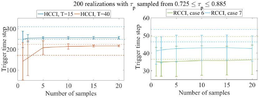
Fig. 12: Plots illustrating the variability of the trigger time steps predicted by the P-indicator and trigger as a function of the number of samples per processors. The data for these plots was generated via 200 realizations of the P-indicator with $\alpha=0.94$, $\beta=0.98$ and $\gamma=0.01$, and with $\tau_{P}$ drawn from $[0.725,0.885]$. The horizontal dashed lines define the range of time steps within which we would like to make the workflow transition (as identified by a domain expert).

Lastly, we performed a series of experiments examining the variation in the trigger time steps as a function of the number of samples used per processor. The data for Fig. 12 was generated via 200 realizations of the P-indicator with $\alpha=0.94$, $\beta=0.98$ and $\gamma=0.01$, and $\tau_{P}$ drawn from $[0.725,0.885]$. The horizontal dashed lines in this figure define the range of true trigger time steps within which we would like to make the workflow transition (as identified by a domain expert). This plot demonstrates that, even across a wide range of $\tau_{P}$ values, with a small number of samples per processor, the quantile sampling approach can accurately estimate the true trigger time steps as defined by the domain expert. The next step will be putting all the pieces together to see how we can predict heat release in situ, within a simulation run.

5 Putting all pieces together: Diagnosing heat release with sublinear algorithms in S3D

The algorithm described in the previous section was deployed in situ for a two-dimensional direct numerical simulation (DNS) of the ethanol HCCI problem (Case HCCI, T=40 in Tab. 2). The DNS was run on half a million grid points with $784$ processors. $20$ points were sampled at random from each processor for the CEMA analysis, generating a total of $15680$ samples for computing the trigger with the P-indicator. The parameters for computing the metric were chosen as follows: $\alpha=0.94$, $\beta=0.98$ and $\gamma=0.01$. This corresponds to less than $4\%$ of the total simulation volume.

Fig. 13 shows the P-indicator being computed in situ inside the simulation code. From top to bottom, the rows show the result when the indicator is computed every $10$, $100$ and $1000$ time steps. As the frequency of computing these indicator increases, the signal tends to get noisier. However, the overall trends and triggers do not change. These images show that our quantile-sampling approach provides a well defined trigger, using $\tau_{P}\in[0.725,0.885]$ and can be used with confidence to predict the rapid rise in the heat release rate that we require to guide temporal and spatial refinement decisions in situ.

As can be inferred from Tab. 3, performing the CEMA analysis on all grid points would increase the cost of the simulation by a factor of $5$, or $400\%$, which is clearly infeasible. Using the sublinear sampling algorithm on the other hand, incurs an overhead of only $1\%$ on the total simulation cost when performed every ten time-steps. The cost savings are even more dramatic in larger, three-dimensional production runs, as the number of samples required does not increase with the number of grid points. Furthermore, we note the cost savings are further increased for larger mechanisms such a primary reference fuel (PRF), composed of a blend of iso-octane and n-heptane. For the PRF mechanism, the CEMA overhead without sublinear sampling would be a factor of $60$ or more. We plan to deploy this algorithm in situ in future large three-dimensional production simulations using S3D, especially with large chemical mechanisms such as PRF.

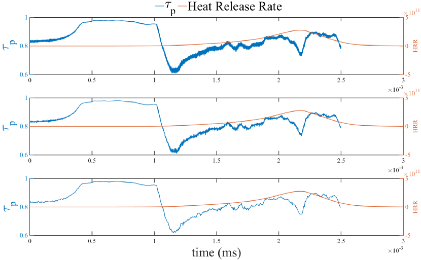
Fig. 13: Plots showing P-indicator being computed every $10$ (top), $100$ (middle) and $1000$ (bottom) time steps.

6 Conclusion

We have proposed an approach for enabling dynamic, adaptive, extreme-scale scientific computing workflows. We introduce the notion of indicators and triggers that are computed in situ, that support data-driven control-flow decisions based on the simulation state. For those indicators and triggers that are computationally prohibitive to compute, we demonstrate how sublinear algorithms enable their estimation with high confidence while incurring extremely low computational overheads.

Throughout this paper, we demonstrate our approach in practice using a proposed indicator to detect changes in the underlying physics of a combustion simulation. The goal of the indicator is to predict rapid heat release in direct numerical simulations of turbulent combustion. We show that chemical explosive mode analysis (CEMA) can be used to devise a noise-tolerant indicator for rapid increase in heat release. Specifically, we study the distribution of CEMA values, and show that heat release is preceded by a decrease in the range of top quantiles in this distribution. We devise an indicator to quantify this intuition and show that it can serve as a robust precursor for heat release. The cost of exhaustive computation of CEMA values dominates the total simulation time, and we propose a sublinear algorithm based on quantile sampling to overcome this computational bottleneck. Our algorithm comes with provable error/confidence bounds, as a function of the number of samples. Most importantly, the number of samples is independent of the problem size, thus our proposed sampling algorithm offers perfect scalability. Our experiments show that our sublinear algorithm is nearly as accurate as an exact algorithm that relies on exhaustive computation, while taking only a fraction of the time. Essentially, sampling in this case provides the algorithmic foundation to turn a critical yet intractable indicator into a practical indicator that takes negligible time. Our experiments on homogeneous charge compression ignition (HCCI) and reactivity controlled compression ignition (RCCI) simulations show that the proposed method can predict heat release, and its computational overhead is negligible.

The impact of this paper is two fold. From the applications’ perspective, we have introduced an important tool that enables adaptive workflows in combustion simulations, an important area of computational science and engineering. Our proposed methods, enable the controlling of mesh granularities, and adaptive I/O frequencies. It is already becoming critically important to have adaptive control over these quantities, but will be crucial as we look ahead to exascale computing. From an algorithmic perspective, our work showcased how sublinear algorithms, a recent development in theoretical computer science can be applied in situ. We believe these algorithmic techniques hold great potential for in situ analysis, and we expect them to be more widely used in the near future.

References

- [1] H. Abbasi, G. Eisenhauer, M. Wolf, K. Schwan, and S. Klasky, Just In Time: Adding Value to The IO Pipelines of High Performance Applications with JITStaging, in Proc. of 20th International Symposium on High Performance Distributed Computing (HPDC’11), June 2011.
- [2] S. Ahern, A. Shoshani, K.-L. Ma, A. Choudhary, T. Critchlow, S. Klasky, V. Pascucci, J. Ahrens, E. W. Bethel, H. Childs, J. Huang, K. Joy, Q. Koziol, G. Lofstead, J. S. Meredith, K. Moreland, G. Ostrouchov, M. Papka, V. Vishwanath, M. Wolf, N. Wright, and K. Wu, Scientific Discovery at the Exascale, a Report from the DOE ASCR 2011 Workshop on Exascale Data Management, Analysis, and Visualization, 2011.
- [3] G. Ballard, T. G. Kolda, A. Pinar, and C. Seshadhri, Diamond sampling for approximate maximum all-pairs dot-product (mad) search, Tech. Report Arxiv:1506.03872, 2015.
- [4] J. C. Bennett, H. Abbasi, P.-T. Bremer, R. Grout, A. Gyulassy, T. Jin, S. Klasky, H. Kolla, M. Parashar, V. Pascucci, P. Pebay, D. Thompson, H. Yu, F. Zhang, and J. Chen, Combining in-situ and in-transit processing to enable extreme-scale scientific analysis, in SC ’12: Proceedings of the International Conference on High Performance Computing, Networking, Storage and Analysis, Salt Lake Convention Center, Salt Lake City, UT, USA, November 10–16, 2012, J. Hollingsworth, ed., pub-IEEE:adr, 2012, IEEE Computer Society Press, pp. 49:1–49:9.
- [5] A. Bhagatwala, J. H. Chen, and T. Lu, Direct numerical simulations of SACI/HCCI with ethanol, Comb. Flame, 161 (2014), pp. 1826–1841.
- [6] A. Bhagatwala, R. Sankaran, S. Kokjohn, and J. H. Chen, Numerical investigation of spontaneous flame propagation under RCCI conditions, Comb. Flame, (Under review).
- [7] J.-M. F. Brad Whitlock and J. S. Meredith, Parallel In Situ Coupling of Simulation with a Fully Featured Visualization System, in Proc. of 11th Eurographics Symposium on Parallel Graphics and Visualization (EGPGV’11), April 2011.
- [8] J. H. Chen, A. Choudhary, B. de Supinski, M. DeVries, E. R. Hawkes, S. Klasky, W. K. Liao, K. L. Ma, J. Mellor-Crummey, N. Podhorski, R. Sankaran, S. Shende, and C. S. Yoo, Terascale direct numerical simulations of turbulent combustion using S3D, Computational Science and Discovery, 2 (2009), pp. 1–31.
- [9] D. Dubhashi and A. Panconesi, Concentration of Measure for the Analysis of Randomized Algorithms, Cambridge University Press, 2009.
- [10] N. Fabian, K. Moreland, D. Thompson, A. Bauer, P. Marion, B. Gevecik, M. Rasquin, and K. Jansen, The paraview coprocessing library: A scalable, general purpose in situ visualization library, in Proc. of IEEE Symposium on Large Data Analysis and Visualization (LDAV), October 2011, pp. 89 –96.
- [11] E. Fischer, The art of uninformed decisions: A primer to property testing, Bulletin of EATCS, 75 (2001), pp. 97–126.
- [12] W. Hoeffding, Probability inequalities for sums of bounded random variables, Journal of the American Statistical Association, 58 (1963), pp. 13–30.
- [13] M. Jha, C. Seshadhri, and A. Pinar, Path sampling: A fast and provable method for estimating 4-vertex subgraph counts, in Proceedings of the 24th International Conference on World Wide Web, WWW ’15, Republic and Canton of Geneva, Switzerland, 2015, International World Wide Web Conferences Steering Committee, pp. 495–505.
- [14] , A space-efficient streaming algorithm for estimating transitivity and triangle counts using the birthday paradox, ACM Trans. Knowl. Discov. Data, 9 (2015), pp. 15:1–15:21.
- [15] S. L. Kokjohn, R. M. Hanson, D. A. Splitter, and R. D. Reitz, Fuel reactivity controlled compression ignition (rcci): A pathway to controlled high-efficiency clean combustion, Int. J. Engine. Res., 12 (2011), pp. 209–226.
- [16] T. G. Kolda, A. Pinar, T. Plantenga, C. Seshadhri, and C. Task, Counting triangles in massive graphs with mapreduce, SIAM Journal on Scientific Computing, 36 (2014), pp. S48–S77.
- [17] T. Lu, C. S. Yoo, J. H. Chen, and C. K. Law, Three-dimensional direct numerical simulation of a turbulent lifted hydrogen flame in heated coflow: a chemical explosive mode analysis, J. Fluid Mech., 652 (2010), pp. 45–64.
- [18] K. Myers, E. Lawrence, M. Fugate, J. Woodring, J. Wendelberger, and J. Ahrens, An in situ approach for approximating complex computer simulations and identifying important time steps, tech. report, 2014. arXiv:1409.0909v1.
- [19] B. Nouanesengsy, J. Woodring, J. Patchett, K. Myers, and J. Ahrens, ADR visualization: A generalized framework for ranking large-scale scientific data using analysis-driven refinement, in Large Data Analysis and Visualization (LDAV), 2014 IEEE 4th Symposium on, IEEE, 2014, pp. 43–50.
- [20] D. Ron, Algorithmic and analysis techniques in property testing, Foundations and Trends in Theoretical Computer Science, 5 (2009), pp. 73–205.
- [21] R. Rubinfeld, Sublinear time algorithms, International Conference of Mathematicians, (2006).
- [22] R. Rubinfeld and M. Sudan, Robust characterization of polynomials with applications to program testing, SIAM Journal of Computing, 25 (1996), pp. 647–668.
- [23] C. Seshadhri, A. Pinar, and T. G. Kolda, Triadic measures on graphs: The power of wedge sampling, in Proceedings of the 2013 SIAM International Conference on Data Mining, 2013, pp. 10–18.
- [24] C. Seshadhri, A. Pinar, and T. G. Kolda, Wedge sampling for computing clustering coefficients and triangle counts on large graphs?, Statistical Analysis and Data Mining, 7 (2014), pp. 294–307.
- [25] R. Shan, C. S. Yoo, J. H. Chen, and T. Lu, Computational diagnostics for n-heptane flames with chemical explosive mode analysis, Comb. Flame, 159 (2012), pp. 3119–3127.
- [26] R. Stevens, A. White, S. Dosanjh, A. Geist, B. Gorda, K. Yelick, J. Morrison, H. Simon, J. Shalf, J. Nichols, and M. Seager, Architectures and technology for extreme scale computing, tech. report, 2009.
- [27] D. Thompson, J. Bennett, C. Seshadhri, and A. Pinar, A provably-robust sampling method for generating colormaps of large data, in Large-Scale Data Analysis and Visualization (LDAV), 2013 IEEE Symposium on, Oct 2013, pp. 77–84.
- [28] V. Vishwanath, M. Hereld, and M. Papka, Toward simulation-time data analysis and i/o acceleration on leadership-class systems, in Proc. of IEEE Symposium on Large Data Analysis and Visualization (LDAV), October 2011.
- [29] H. Yu, C. Wang, R. W. Grout, J. H. Chen, and K.-L. Ma, In-situ visualization for large-scale combustion simulations, IEEE Computer Graphics and Applications, 30 (2010), pp. 45–57.