Greedy Is an Almost Optimal Deque

Abstract

In this paper we extend the geometric binary search tree (BST) model of Demaine, Harmon, Iacono, Kane, and Pǎtraşcu (DHIKP) to accommodate for insertions and deletions. Within this extended model, we study the online Greedy BST algorithm introduced by DHIKP.  Greedy BST is known to be equivalent to a maximally greedy (but inherently offline) algorithm introduced independently by Lucas in 1988 and Munro in 2000, conjectured to be dynamically optimal.

With the application of forbidden-submatrix theory, we prove a quasilinear upper bound on the performance of Greedy BST on deque sequences. It has been conjectured (Tarjan, 1985) that splay trees (Sleator and Tarjan, 1983) can serve such sequences in linear time. Currently neither splay trees, nor other general-purpose BST algorithms are known to fulfill this requirement. As a special case, we show that Greedy BST can serve output-restricted deque sequences in linear time. A similar result is known for splay trees (Tarjan, 1985; Elmasry, 2004).

As a further application of the insert-delete model, we give a simple proof that, given a set $U$ of permutations of $[n]$, the access cost of any BST algorithm is $\Omega(\log|U|+n)$ on “most” of the permutations from $U$. In particular, this implies that the access cost for a random permutation of $[n]$ is $\Omega{(n\log{n})}$ with high probability.

Besides the splay tree noted before, Greedy BST has recently emerged as a plausible candidate for dynamic optimality. Compared to splay trees, much less effort has gone into analyzing Greedy BST. Our work is intended as a step towards a full understanding of Greedy BST, and we remark that forbidden-submatrix arguments seem particularly well suited for carrying out this program.

1 Introduction

Binary search trees (BST) are among the most popular and most thoroughly studied data structures for the dictionary problem. There remain however, several outstanding open questions related to the BST model. In particular, what is the best way to adapt a BST in an online fashion, in reaction to a sequence of operations (e.g. access, insert, and delete), and what are the theoretical limits of such an adaptation? Does there exist a “one-size-fits-all” BST algorithm, asymptotically as efficient as any other dynamic BST algorithm, regardless of the input sequence?

Splay trees have been proposed by Sleator and Tarjan [13] as an efficient BST algorithm, and were shown to be competitive with any static BST (besides a number of other attractive properties, such as the balance, working set, and static finger properties). Furthermore, Sleator and Tarjan conjectured splay trees to be competitive with any dynamic BST algorithm; this is the famous dynamic optimality conjecture [13]. An easier, but similarly unresolved, question asks whether such a dynamically optimal algorithm exists at all. We refer to [7] for a survey of work related to the conjecture.

A different BST algorithm (later called GreedyFuture) has been proposed independently by Lucas [8] and by Munro [9]. GreedyFuture is an offline algorithm: it anticipates future accesses, preparing for them according to a greedy strategy. In a breakthrough result, Demaine, Harmon, Iacono, Kane, and Pǎtraşcu (DHIKP) transformed GreedyFuture into an online algorithm (called here Greedy BST), and presented a geometric view of BST that facilitates the analysis of access costs (while abstracting away many details of the BST model).

At present, our understanding of both splay trees and Greedy BST is incomplete. For splay trees, besides the above-mentioned four properties (essentially subsumed by a single statement called the access lemma), a few other corollaries of dynamic optimality have been shown, including the sequential access [15] and the dynamic finger [2, 1] theorems. The only known proof of the latter result uses very sophisticated arguments, which makes one pessimistic about the possibility of proving even stronger statements.

A further property conjectured for splay trees is a linear cost on deque sequences (stated as the “deque conjecture” by Tarjan [15] in 1985). Informally, a deque sequence consists of insert and delete operations at minimum or maximum elements of the current dictionary. Upper bounds for the cost of splay on a sequence of $n$ deque operations are $O(n\alpha(n))$ by Sundar [14] and $O(n\alpha^{\ast}(n))$ by Pettie [10]. Here $\alpha$ is the extremely slowly growing inverse Ackermann function, and $\alpha^{\ast}$ is its iterated version. A linear bound for splay trees on output-restricted deque sequences (i.e. where deletes occur only at minima) has been shown by Tarjan [15], and later improved by Elmasry [5].

In general, our understanding of Greedy BST is even more limited. Fox [6] has shown that Greedy BST satisfies the access lemma and the sequential access theorem, but no other nontrivial bounds appear to be known. One might optimistically ascribe this to a (relative) lack of trying, rather than to insurmountable technical obstacles. This motivates our attempt at the deque conjecture for Greedy BST.

As mentioned earlier, a deque sequence consists of insert and delete operations. In the tree-view, e.g. for splay trees, such operations have a straightforward implementation. Unfortunately, the geometric view in which Greedy BST can be most naturally expressed only concerns with accesses. Thus, prior to our work there was no way to formulate the deque conjecture in a managable way for Greedy BST.

Our contributions.

We augment the geometric model of DHIKP to allow insert and delete operations (exemplified by the extension of the Greedy BST algorithm), and we show the offline and online equivalence of a sequence of operations in geometric view with the corresponding sequence in tree-view. This extended model allows us to formulate the deque conjecture for Greedy BST. We transcribe the geometric view of Greedy BST in matrix form, and we apply the forbidden-submatrix technique to derive the quasilinear bound $O(m2^{\alpha(m,m+n)}+n)$ on the cost of Greedy BST, while serving a deque sequence of length $m$ on keys from $[n]$.

We also prove an $O(m+n)$ upper bound for the special case of output-restricted deque sequences. We find this proof considerably simpler than the corresponding proofs for splay trees, and we observe that a slight modification of the argument gives a new (and perhaps simpler) proof of the sequential access theorem for Greedy BST.

As a further application of the insert-delete model we show through a reduction to sorting that for any BST algorithm, most representatives from a set $U$ of permutations on $[n]$ have an access cost of $\Omega(\log{|U|}+n)$. In particular, this implies that a random permutation of $[n]$ has access cost $\Omega(n\log{n})$ with high probability. A similar result has been shown by Wilber [16] for random access sequences (that might not be permutations). Our proof is self-contained, not relying on Wilber’s BST lower bound. Permutation access sequences are important, since it is known that the existence of a BST algorithm that is constant-competitive on permutations implies the existence of a dynamically optimal algorithm (on arbitrary access sequences).

Related work.

A linear cost for deque sequences is achieved by the multi-splay algorithm [4, Thm 3] in the special case when the initial tree is empty; by contrast, the results in this paper make no assumption on the initial tree.

Most relevant to our work is the deque bound of Pettie for splay trees [10]. That result relies on bounds for Davenport-Schinzel sequences, which can be reformulated in the forbidden-submatrix framework. Indeed, the use of forbidden-submatrix theory for proving data structure bounds was pioneered by Pettie, who reproved the sequential access theorem for splay trees [11] (among other data structure results). Our application of forbidden-submatrix theory is somewhat simpler and perhaps more intuitive: the geometric view of Greedy BST seems particularly suitable for these types of arguments, as the structure of BST accesses is readily available in a matrix form, without the need for an extra “transcribing” step.

2 Geometric Formulation of BST with Insertion/Deletion

In this section we extend the model of DHIKP [3] to allow for insertions and deletions. After defining our geometric model, we prove the equivalence of the arboreal (i.e. tree-view) and the geometric views of BSTs.

2.1 Rotations and Updates

Definition 1 (Valid Reconfiguration)

Given a BST $T_{1}$, a (connected) subtree $\tau$ of $T_{1}$ containing the root, and a tree $\tau^{\prime}$ on the same nodes as $\tau$, except that one node may be missing or newly added, we say that $T_{1}$ can be reconfigured by an operation $\tau\rightarrow\tau^{\prime}$ to another BST $T_{2}$ if $T_{2}$ is identical to $T_{1}$ except for $\tau$ being replaced by $\tau^{\prime}$, meaning that the child pointers of elements not in $\tau$ do not change. The cost of the reconfiguration is $\max\{|\tau|,|\tau^{\prime}|\}$.

This definition differs from [3, Def.2] in that $\tau^{\prime}$ need not be defined on the same nodes as $\tau$. Note that, according to the definition, if an operation $\tau\rightarrow\tau^{\prime}$ changes a child pointer of an element $x$, then $x\in\tau$. See Figure 1 for examples.

Definition 2 (Execution of Update Sequence)

Given an update sequence

$$S=\langle(s_{1},\mathtt{op}_{1}),(s_{2},\mathtt{op}_{2}),\dots,(s_{m},\mathtt{op}_{m})\rangle,\text{ where }\mathtt{op}_{i}\in\{\mathtt{access},\mathtt{insert},\mathtt{delete}\},$$

we say that a BST algorithm executes $S$ by an execution $E=\langle T_{0},\tau_{1}\rightarrow\tau_{1}^{\prime},\dots,\tau_{m}\rightarrow\tau_{m}^{\prime}\rangle$ if all reconfigurations $\tau_{t}\rightarrow\tau_{t}^{\prime}$ transforming $T_{t-1}$ to $T_{t}$ are valid, and for all $t$

• if $\mathtt{op}_{t}=\mathtt{access},$ then $s_{t}\in\tau_{t}$ and $\tau_{t}^{\prime}=\tau_{t}$ as a set,

• if $\mathtt{op}_{t}=\mathtt{insert},$ then $\tau_{t}^{\prime}=\{s_{t}\}\dot{\cup}\tau_{t}$ as a set,

• if $\mathtt{op}_{t}=\mathtt{delete},$ then $\tau_{t}=\{s_{t}\}\dot{\cup}\tau_{t}^{\prime}$ as a set.

We also say that $E$ executes $S$. The cost of execution of $E$ is the sum over all reconfiguration costs. If an element $x\in\tau_{t}\cup\tau_{t}^{\prime}$, we say that $x$ is touched at time $t$.

Figure 1: (left) Examples of valid insert/delete operations. Circled elements indicate $\tau$ and $\tau^{\prime}$; (right) Examples of invalid operations: $\tau$ does not contain root (above) and $\tau^{\prime}$ cannot link all pendant trees (below).

We assume that we work over the set $[n]$. Each element can be inserted or deleted many times, but insertions and deletions on the same element must be alternating. We also assume that every element is accessed or updated at least once.

2.2 Valid Sets

Definition 3 (Geometric View of Update Sequence)

The geometric view of an update sequence $S$ is a point set $P(S)=A(S)\dot{\cup}I(S)\dot{\cup}D(S)$ in the integer grid $[n]\times[m]$ consisting of access points $A(S)=\{(s_{t},t)\mid\mathtt{op}_{t}=\mathtt{access}\}$, insertion points $I(S)=\{(s_{t},t)\mid\mathtt{op}_{t}=\mathtt{insert}\}$, and deletion points $D(S)=\{(s_{t},t)\mid\mathtt{op}_{t}=\mathtt{delete}\}$. Update points are $U(S)=I(S)\dot{\cup}D(S)$.

We usually omit the parameter $S$ and simply write $A,I,D,U$ when the choice of $S$ is clear from context. We denote the $x$-coordinate and $t$-coordinate of a point $p$ by $(p_{x},p_{t})$. By element $x$, we mean the column $x$. By time $t$, we mean the row $t$.

Definition 4 (Valid Point)

Given a point set $P(S)$ in the integer grid $[n]\times[m]$, let $p$ be a point ($p$ may not be in $P(S)$), and let $p^{\prime},p^{\prime\prime}\in U(S)$ denote the update points nearest to $p$, below (resp. above) $p$, i.e. $p^{\prime}_{x}=p^{\prime\prime}_{x}=p_{x}$, and $p^{\prime}_{t}<p_{t}<p^{\prime\prime}_{t}$. One or both of $p^{\prime}$ and $p^{\prime\prime}$ might not exist. We say that $p$ is valid in $P(S)$, iff:

• $p\notin U(S)$, $p^{\prime}\in I(S)$ (or does not exist), and $p^{\prime\prime}\in D(S)$ (or does not exist), or

• $p\in I(S)$, $p^{\prime}\in D(S)$ (or does not exist), and $p^{\prime\prime}\in D(S)$ (or does not exist), or

• $p\in D(S)$, $p^{\prime}\in I(S)$ (or does not exist), and $p^{\prime\prime}\in I(S)$ (or does not exist).

Let $T_{t}$ denote the resulting tree at time $t$ during an execution of the BST algorithm $E$ on the update sequence $S$. Observe that Definition 4 allows elements to be accessed or deleted without having been inserted before. Such elements are (implicitly) in the initial tree $T_{0}$.

Fact 2.1

A point $x$ can be touched at time $t$ iff $(x,t)$ is valid.

Suppose that $(x,t)$ is valid. If $(x,t)$ is a deletion point, then $x$ is in $T_{t-1}$ but not $T_{t}$, and it is touched. If $(x,t)$ is an insertion point, then $x$ is in $T_{t}$ but not $T_{t-1}$, and it is touched. If $(x,t)$ is not an update point, then $x$ is in both trees, and might or might not be touched. See Figure 2 for an illustration.

Definition 5 (Predecessor/Successor of a Point)

Given $P(S)$, the predecessor ${\mathit{pred}}(p)$ of a point $p$ is the largest element $x^{\prime}$ smaller than $p_{x}$ such that $(x^{\prime},p_{t})$ is valid. We also write ${\mathit{pred}}(p)=(x^{\prime},p_{t})$ as a point. The successor $\mathit{succ}(p)$ of $p$ is symmetrically defined.

Definition 6 (Valid Set)

A point set $P\supseteq P(S)$ is valid iff every point $p\in P$ is valid.

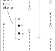
Figure 2: A point set with insert ($\ocircle$) and delete ($\times$) points. Dashed lines indicate valid points. Observe that $\mathit{succ}(x)=v_{3}$, $\mathit{succ}(y)=v_{2}$, and ${\mathit{pred}}(x)={\mathit{pred}}(y)=v_{1}$.

For any node $x$ in a tree $T$, let ${\mathit{pred}}_{T}(x)$ and $\mathit{succ}_{T}(x)$ denote the predecessor, respectively successor of $x$ in $T$. The following lemma shows that points in a valid set, and their predecessor and successor, are associated with nodes in the tree at the corresponding time.

Lemma 1

Let $P\supseteq P(S)$ be a valid point set, and $E$ executes $S$. For any $p\in U(S)$, we have ${\mathit{pred}}(p)={\mathit{pred}}_{T_{p_{t}}}(p_{x})$ and $\mathit{succ}(p)=\mathit{succ}_{T_{p_{t}}}(p_{x})$.

Proof

Let $x^{\prime}={\mathit{pred}}(p)$ and hence $(x^{\prime},p_{t})$ is valid by definition. By Fact 2.1, $x^{\prime}$ can be touched at time $p_{t}$. Since $x^{\prime}$ is not an updated element, we have $x^{\prime}\in T_{p_{t}}$. Moreover, $x^{\prime}$ is the closest element on the left of $p_{x}$ at this time. So $x^{\prime}={\mathit{pred}}_{T_{p_{t}}}(p_{x})$. The proof for successor is symmetric.

Definition 7 (Active Time of Points)

Let $p$ be a point in a valid point set $P\supseteq P(S)$. The active time $act(p)$ of $p$ is the maximal consecutive interval of time $[t_{ins}(p),t_{del}(p)]$ containing $p_{t}$ such that, for all $t\in act(p)$, $(p_{x},t)$ is valid. We call $t_{ins}(p)$ insertion time of $p$, and $t_{del}(p)$ deletion time of $p$.

2.3 Arboreally Satisfied Set

Definition 8 (Geometric View of BST Execution)

The geometric view of a BST execution $E=\langle T_{0},\tau_{1}\rightarrow\tau_{1}^{\prime},\dots,\tau_{m}\rightarrow\tau_{m}^{\prime}\rangle$ of some update sequence $S$ is the point set $P(E)=\{(x,t)\mid x\in\tau_{t}\cup\tau_{t}^{\prime}\}$ in the integer grid, indicating which element is touched at which time. Note that $P(E)\supseteq P(S)$.

Definition 9 (Arboreally Satisfied Set)

A valid point set $P\supseteq P(S)$ is (arboreally) satisfied iff the following holds:

• For each pair $p,q\in P$ that are both active from time $p_{t}$ to $q_{t}$ (called an active pair), either both $p$ and $q$ lie in the same vertical/horizontal line, or there is a point $r\in\square_{pq}\cap P\setminus\{p,q\}$. If $r$ is on the bottommost row of $\square_{pq}$, then $r$ cannot be a deletion point. If $r$ is on the topmost row of $\square_{pq}$, then $r$ cannot be an insertion point.

• For each update point $p\in U$, if both ${\mathit{pred}}(p)$ and $\mathit{succ}(p)$ exist, then either ${\mathit{pred}}(p)$ or $\mathit{succ}(p)$ is also in $P$.

The first condition is almost the same as the one in [3, Def. 2.3] but focused only on active pairs (they are active from $p_{t}$ to $q_{t}$), and with additional technical condition due to update points. The second condition says that if the updated element is not the current minimum/maximum, then one of its adjacent elements must be touched.

Note that if there are no update points, then all points are active the whole time and our definition is equivalent to [3, Def. 2.3]. We defer the proof of the following fact to the appendix.

Fact 2.2

Suppose that $P$ is satisfied. Then, for each pair $p,q\in P$ which are both active from time $p_{t}$ to $q_{t}$ and $p_{t}<q_{t}$, there exists a point in $P\setminus\{p,q\}$ on a side of $\square_{pq}$ incident to $p$, that is either a non-deletion point, or the corner $(p_{x},q_{t})$. Similarly, there exists a point in $P\setminus\{p,q\}$ on a side of $\square_{pq}$ incident to $q$, that is either a non-insertion point, or the corner $(q_{x},p_{t})$.

3 Equivalence of Arboreal and Geometric Views

In this section we prove the following theorem:

Theorem 3.1

A point set $P$ is satisfied iff $P=P(E)$ for some BST execution $E$.

The first direction of the proof involves considering a BST algorithm and showing that it generates a satisfied point set (tree to geometry). The second direction is showing how to convert a satisfied point set to a BST algorithm (geometry to tree).

3.1 Tree to Geometry

Lemma 2

Let $x$ and $z$ be elements with consecutive values in a BST $T$, with $x<z$. Then one of $x$ and $z$ is an ancestor of the other.

Proof

Suppose not. Then the lowest common ancestor of $x$ and $z$ is another element $y$. We know $x<y<z$ which is a contradiction.

Lemma 3

Suppose that $y$ is not the minimum or maximum element in a BST $T$. To insert or delete $y$ in $T$, either ${\mathit{pred}}_{T}(y)$ or $\mathit{succ}_{T}(y)$ must be touched.

Lemma 4

For any execution $E$, a point set $P(E)$ is satisfied.

Proof

There are two conditions that need to be checked.

For the first condition, let $p,q$ be a pair of points in $P(E)$ active from time $p_{t}$ to $q_{t}$. Suppose that $p,q$ violate the condition. Hence, they are not vertically or horizontally aligned. We assume that $p_{t}<q_{t}$ and $p_{x}<q_{x}$. Since $p_{x}$ and $q_{x}$ are active at time $p_{t}$, by Fact 2.1 and the statement below the fact, they exist in the tree $T_{p_{t}}$. Hence, a lowest common ancestor $a$ of $p_{x}$ and $q_{x}$ in $T_{p_{t}}$ is well-defined. There are two cases.

If $a=p_{x}$, then $p_{x}$ is an ancestor of $q_{x}$. Since $\square_{pq}$ is not satisfied, $q_{x}$ is not touched from time $p_{t}$ to $q_{t}-1$ and $p_{x}$ remains an ancestor of $q_{x}$ right before time $q_{t}$. Thus, to touch $q_{x}$ at time $q_{t}$, $p_{x}$ must be touched, and so $(p_{x},q_{t})\in\square_{pq}$. Only insertion point can be in the topmost row of unsatisfied $\square_{pq}$. So $(p_{x},q_{t})$ an insertion point. But this implies that $p$ and $q$ are not active pair, which is a contradiction.

If $a\neq p_{x}$, then $a$ must be touched at time $p_{t}$. As $a$ has value between $p_{x}$ and $q_{x}$, we have $(a,p_{t})\in\square_{pq}$. Since $\square_{pq}$ is not satisfied, $(a,p_{t})$ is a deletion point and, moreover, $p_{x}$ must be its predecessor. Hence $p_{x}$ becomes an ancestor of $q_{x}$ right after time $p_{t}$ and we can use the previous argument again.

For the second condition, suppose that $p\in U$ is an update point. That is, we update $p_{x}$ in the BST $T_{p_{t}}$. If both ${\mathit{pred}}(p)$ and $\mathit{succ}(p)$ exist, then $p_{x}$ is not a minimum or maximum in $T_{p_{t}}$. By Lemma 3, either ${\mathit{pred}}_{T_{p_{t}}}(p_{x})$ or $\mathit{succ}_{T_{p_{t}}}(p_{x})$ is touched at time $p_{t}$. By Lemma 1, ${\mathit{pred}}_{T_{p_{t}}}(p_{x})={\mathit{pred}}(p)$ and $\mathit{succ}_{T_{p_{t}}}(p_{x})=\mathit{succ}(p)$, and we are done.

3.2 Geometry to Tree

Now we show how to convert a valid point set to an offline algorithm first. We need the following lemma, which is essentially a converse of Lemma 3, saying that if we touch either ${\mathit{pred}}_{T}(y)$ or $\mathit{succ}_{T}(y)$, then we can insert or delete $y$. We defer the proofs of the following two statements to the appendix.

Lemma 5

Suppose either ${\mathit{pred}}_{T}(y)$ or $\mathit{succ}_{T}(y)$ is in a subtree $\tau$ containing the root of $T$, or $y$ is the minimum or maximum element in $T$. Then (i) any reconfiguration $\tau\rightarrow\tau^{\prime}$, where $\tau^{\prime}=\tau\dot{\cup}\{y\}$ as a set, is valid, and (ii) any reconfiguration $\tau\rightarrow\tau^{\prime}$, where $\tau=\tau^{\prime}\dot{\cup}\{y\}$ as a set, is valid.

Lemma 6 (Offline Equivalence)

For any satisfied set $X$, there is a point set $P(E)=X$ for some execution $E$. We call $E$ a tree view of $X$.

By Lemma 4 and 6, this concludes the proof of Theorem 3.1.

Observe that if $X=P(E)$, the quantity $|X|$ is exactly the execution cost of $E$.

3.3 Geometry to Tree: Online

The discussion in § 3.2 assumes that a satisfied set $X$ is available all at once, and we show that there exists an execution $E$ (i.e. an offline BST algorithm) whose point set $P(E)$ is exactly $X$.

We call an online geometric algorithm an algorithm that, given a geometric update sequence $P(S)\subseteq[n]\times[m]$, outputs a satisfied superset $P\supseteq P(S)$, with the condition that both the input and output are revealed row-by-row (i.e. the decision on which points to touch can depend only on the current and preceding rows of the input). We remark that Greedy BST (as extended in § 4) is such an algorithm.

Analogously, by an online BST algorithm we mean a procedure that, given an initial set $S_{0}\subseteq[n]$, and an update sequence $S$, outputs an execution $E$, with the condition that both the input and output are revealed item-by-item (i.e. the decision on which reconfiguration to perform can depend only on the current and preceding update operations).

Theorem 3.2 (Online Equivalence)

For any online geometric algorithm $\mathcal{A}$, there exists an online BST algorithm $\mathcal{A^{\prime}}$ such that, on any update sequence, the cost of $\mathcal{A^{\prime}}$ is bounded by a constant times the cost of $\mathcal{A}$.

The proof of Theorem 3.2 is an adaptation of the proof of Lemma $2.3$ in [3] to the new geometric setting, and is analogous to the proof of Lemma 6. We omit the proof in this extended abstract.

4 Defining Greedy BST with Insertion/Deletion

Greedy BST is an online algorithm for constructing a satisfied set given an update sequence $S$. At each time $t$, Greedy BST minimally satisfies the point set up to time $t$. Having defined satisfied sets when there are update points, we naturally obtain the extension of Greedy BST that can handle insertions and deletions.

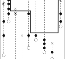
Figure 3: A Greedy BST execution with insert ($\ocircle$), delete ($\times$), access ($\odot$), touched ($\newmoon$) points, and touched points at time $p_{t}$ ($\Diamondblack$). Thick line shows stair of $p$. Observe that a non-(min/max) insert or delete must access a neighbor as well.

We develop some notation for describing the algorithm. A rectangle $\square_{pq}$ is unsatisfied if there is no other point in the proper (closed) rectangle formed by points $p$ and $q$. We say that $p$ and $q$ are an active pair if they are active from time $p_{t}$ to $q_{t}$. The stair of point $p$ is denoted by ${\mathit{stair}}(p)=\{p\}\cup\{q\mid\square_{pq}$ is unsatisfied rectangle formed by an active pair $p$ and $q$ where $q$ is below $p\}$. The stair of element $x$ at time $t$ is the stair of the point $(x,t)$. Satisfying/touching ${\mathit{stair}}(x,t)$ means visiting/touching, at time $t$, the elements of points in the stair: $\{(q_{x},t)\mid q\in{\mathit{stair}}(x,t)\}$. These elements are then added to the row at time $t$.

Fact 4.1

Touching the stair ${\mathit{stair}}(p)$ is to minimally satisfy the point $p$.

Therefore, when Greedy BST gets an access point $p$, it touches only ${\mathit{stair}}(p)$. For an update point $p$, if $p$ is not the minimum or maximum, then Greedy BST chooses the smaller set between ${\mathit{stair}}(p)\cup{\mathit{stair}}({\mathit{pred}}(p))$ and ${\mathit{stair}}(p)\cup{\mathit{stair}}(\mathit{succ}(p))$. This is because of the second condition of satisfied set. If $p$ is the minimum or maximum, then Greedy BST just touches ${\mathit{stair}}(p)$. The execution of Greedy BST is illustrated in Figure 3.

The following observation is useful for deque sequences. For insertion point $p$, observe that ${\mathit{stair}}(p)=\{p\}$ because the active time of $p$ begins at time $p_{t}$ itself (for any point $q$ below $p$, $p$ and $q$ are not an active pair by definition).

Fact 4.2

To insert $p$ such that $p$ is the minimum or maximum, Greedy BST touches only $p$.

5 Performance of Greedy BST on Deque Sequences

Definition 10 (Deque Sequence)

An update sequence is a deque sequence if it has only insertions and deletions at the current minimum or maximum element, and no access operations.

Definition 11 (Output-restricted)

A deque sequence is output-restricted if it has deletions only at minimum elements.

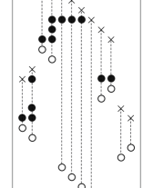
Figure 4: Sample execution of Greedy BST on a concentrated deque sequence with insert ($\ocircle$), delete ($\times$), and touched ($\newmoon$) points. Dashed lines show the active times of elements.

Theorem 5.1

The cost of executing a deque sequence on $[n]$ of length $m$ by Greedy BST is at most $O(m2^{\alpha(m,n+m)}+n)$, where $\alpha$ is the inverse Ackermann function.

Theorem 5.2

The cost of executing an output-restricted deque sequence on $[n]$ of length $m$ by Greedy BST is at most $24m+12n$.

Remark.

The bound in Theorem 5.2 refers to the cost of the online geometric Greedy BST. In the online tree-view equivalent the constants can be larger, hinging on the details of Theorem 3.2, but the bound remains of the form $O(m+n)$.

The rest of this section is devoted to the proofs of Theorems 5.1 and 5.2.

5.1 Concentrated Deque Sequences

We first reduce the analysis of Greedy BST on any deque sequence to that on a special type of deque sequence that we call a concentrated deque sequence. Recall that in a deque sequence we can delete only the current minimum or maximum. We define two sets of elements as follows: let $L_{t}$ be the set of elements which are deleted (from the left) before time $t$ when they were the minimum at their deletion time, and $R_{t}$ be the set of elements which are deleted (from the right) before time $t$ when they were not the minimum at their deletion time. Observe that $L_{t}\cap R_{t}=\varnothing$.

Definition 12 (Concentrated Deque Sequence)

A deque sequence is concentrated if, for any time $t$, if the inserted element $x$ is the minimum, then $y<x$ for all $y\in L_{t}$, and if $x$ is the maximum, then $x<y$ for all $y\in R_{t}$.

Note that the definition implies that each element in a concentrated deque sequence can be inserted and deleted at most once. We defer the proof of the following lemma to the appendix.

Lemma 7

For any deque sequence $S$, there is a concentrated deque sequence $S^{\prime}$ such that the execution of any BST algorithm on $S^{\prime}$ and $S$ have the same cost.

5.2 Greedy BST on a Concentrated Deque Sequence

Now we analyze the performance of Greedy BST on concentrated deque sequences (see Figure 4 for an example). Because of Lemma 7, we can view the points touched by Greedy BST as an $(m\times(n+m))$ binary matrix (i.e. with entries $0$ and $1$), with all touched points represented as ones, and all other grid elements as zeroes. Notice that the number of columns is $n+m$ instead of $n$ because of the reduction in Lemma 7 which allows each element to be inserted and deleted at most once. We further observe that if a deque sequence is output-restricted, then the transformation of Lemma 7 yields a concentrated deque sequences that is similarly output-restricted.

Definition 13 (Forbidden Pattern)

A binary matrix $M$ is said to avoid a binary matrix $P$ (called a pattern) if there exists no submatrix $M^{\prime}$ of $M$ with same dimensions as $P$, such that for all $1$-entries of $P$, the corresponding entry in $M^{\prime}$ is $1$ (the $0$-entries of $P$ are “don’t care” values).

We denote by $\mathrm{Ex}(P,m,n)$ the largest number of $1$s in an $(m\times n)$ matrix $M$ that avoids pattern $P$. In this work, we refer to the following patterns (as customary, we write dots for $1$-entries and empty spaces for $0$-entries).

$$P_{5}=\left(\begin{matrix}\bullet&\ &\bullet&\ &\bullet\\ \ &\bullet&\ &\bullet&\ \end{matrix}\right)\quad and\quad P_{4}=\left(\begin{matrix}\bullet&\ &\ &\ \\ \ &\ &\bullet&\ \\ \ &\bullet&\ &\ \\ \ \ &\ &\ &\bullet\\ \end{matrix}\right)$$

Lemma 8

The execution of Greedy BST on concentrated deque sequences avoids the pattern $P_{5}$.

Proof

Suppose that $P_{5}$ appears in the Greedy BST execution, and name the touched points matched to the $1$-entries in $P_{5}$ from left to right as $a,b,c,d,$ and $e$.

Let $t>b_{t}$ be smallest such that $(c_{x},t)$ is touched. Then $t\leq c_{t}$ and either $b$ or $d$ must have been deleted within the time interval $[b_{t},t]$. Otherwise, any update point in the interval $[b_{t},t]$ is outside the interval $[b_{x},d_{x}]$ and $c_{x}$ is “hidden” by $b$ and $d$ (it cannot be on the stair of any update point).

Assume w.l.o.g. that $b$ is deleted. If $b$ is deleted by a minimum-delete, then $a$ cannot be touched. If $b$ is deleted by a maximum-delete, then $e$ cannot be touched. This is because the sequence is concentrated.

Lemma 9

The execution of Greedy BST on concentrated output-restricted deque sequences avoids the pattern $P_{4}$.

Proof

Suppose that $P_{4}$ appears in the Greedy BST execution, and name the touched points matched to the $1$-entries in $P_{4}$ from left to right as $a,b,c,$ and $d$. We claim that in order to touch $c$, there has to be a deletion point in the interval $[b_{x},d_{x}]$ in the time interval $[d_{t},c_{t}]$. Otherwise, any deletion point in the time interval $[d_{t},c_{t}]$ is left of $b_{x}$ (as deletes happen only at the minimum). Furthermore, all insertion points in the time interval $[b_{t},c_{t}]$ must be outside of $[b_{x},d_{x}]$ (since both $b$ and $d$ are active at time $b_{t}$). We remind that insertion touches nothing else besides the insertion point itself. This means that $c$ cannot be touched: it is “hidden” to deletion points on the left of $b_{x}$ by $b$.

Denote the deletion point in the rectangle $[b_{x},d_{x}]\times[d_{t},c_{t}]$ as $d^{\prime}$. Observe that $a$ is to the left of and above $d^{\prime}$, and since we only delete minima, $a$ is not active at time $d^{\prime}_{t}$. In order to be touched, $a$ must become active after $d^{\prime}_{t}$ via an insertion, contradicting that the sequence is concentrated.

Fact 5.3

(​ [12, Thm $3.4$] ).  $\mathrm{Ex}(P_{5},u,v)=O(u2^{\alpha(u,v)}+v)$.

Fact 5.4

(​ [12, Thm $1.5(5)$] ).  $\mathrm{Ex}(P_{4},u,v)<12(u+v)$.

Proof of Theorem 5.1:

By Lemma 7, it is enough to analyze the cost of Greedy BST on concentrated deque sequences. This cost is bounded by $O(m2^{\alpha(m,m+n)}+n)$ using Lemma 8 and Fact 5.3.

Proof of Theorem 5.2:

By Lemma 7, it is enough to analyze the cost of Greedy BST on concentrated deque sequences. This cost is bounded by $24m+12n$ using Lemma 9 and Fact 5.4.

Remark.

The proof of Theorem 5.2 can be minimally adjusted to prove the sequential access theorem for Greedy BST. Sequential access can be simulated as a sequence of minimum-deletions. In this way we undercount the cost by exactly one touched point above each access, which adds a linear term to the bound.

6 A Lower Bound on Accessing a Set of Permutations

Let $U$ be a set of permutations on $[n]$. In this section we prove the following theorem:

Theorem 6.1

Fix a BST algorithm $\mathcal{A}$ and a constant $\epsilon<1$. There exists $U^{{}^{\prime}}\subseteq U$ of size $|U^{{}^{\prime}}|\geq(1-\frac{1}{{|U|}^{\epsilon}})|U|$ such that $\mathcal{A}$ requires $\Omega(\log|U|+n)$ access cost on any permutation in $U^{{}^{\prime}}$.

Proof

The proof utilizes the geometric view of insertions, and uses two reductions. We first claim that there exists an algorithm $\mathcal{B}$ that is capable of insertions such that the cost of $\mathcal{A}$ to access a permutation $\pi$ is no less than the cost of $\mathcal{B}$ to insert $\pi$. Note that since $\mathcal{A}$ is accessing $\pi$, all the points are active by definition. We will describe $\mathcal{B}$ in the geometric view simply by requiring that upon inserting $\pi(t)$ at time $t$, $\mathcal{B}$ touches all the points that $\mathcal{A}$ touches while accessing $\pi(t)$ at time $t$. Note that $\mathcal{A}$ touches at least all the points in ${\mathit{stair}}(\pi(t),t)$, and $\mathcal{B}$ is required only to touch either ${\mathit{pred}}(\pi(t))$ and its stair, or $\mathit{succ}(\pi(t))$ and its stair (Definition $11$). Since ${\mathit{pred}}(\pi(t))$ belongs to ${\mathit{stair}}(\pi(t),t)$, one easily sees that ${\mathit{stair}}({\mathit{pred}}(p))\subset{\mathit{stair}}(\pi(t),t)$, and this defines a valid insertion algorithm.

We now reduce $\mathcal{B}$ to an algorithm for sorting $\pi$. Just by a traversal of the tree maintained by $\mathcal{B}$ at time $n$, we can produce the sorted order of $\pi$ after incurring a cost of $O(n)$. However, we know that to sort a set $U$ of permutations, any (comparison-based) sorting algorithm must require $\Omega(\log|U|+n)$ comparisons on at least a $1-\frac{1}{{|U|}^{\epsilon}}$ fraction of the permutations in $U$. To see this, note that the decision tree of any sorting algorithm must have at least $|U|$ leaves (note that here we are assuming the weaker hypothesis that $\mathcal{A}$ and hence the sorting algorithm, are only designed to work on $U$; they may fail outside $U$). The number of leaves at height at most $(1-\epsilon)\log|U|$ is at most ${|U|}^{1-\epsilon}$, and hence at least a $1-\frac{1}{{|U|}^{\epsilon}}$ fraction require at least $(1-\epsilon)\log|U|=\Omega(\log|U|)$ comparisons. Adding the trivial bound of $\Omega(n)$ to scan the input permutation gives us the desired bound.

Remark.

Upper bounds proved for our model do not directly translate into bounds for algorithms. For example, when a new maximum is inserted, this can be done at a cost of one by making the element the root of the tree, respectively, only touching the element inserted. Note that this requires the promise that the element inserted is actually a new maximum. A slight extension makes the model algorithmic. This is best described in tree-view. We put all nodes of the tree in in-order into a doubly-linked list. Then, in the case of an insertion one can actually stop the search once the predecessor or the successor of the new element has been reached in the search because by also comparing the new element with the neighboring list element, one can verify that a node contains the predecessor or successor. Thus at the cost of a constant factor, bounds proved for our model are algorithmic.

Acknowledgement.

We thank an anonymous reviewer for valuable comments.

Appendix 0.A Proof Omitted from Section 2

0.A.1 Proof of Fact 2.2

We give the proof only for $p$, as it is symmetric for $q$.

Since $P$ is satisfied, there is a point $r$ in $\square_{pq}\cap P\setminus\{p,q\}$ that satisfies $\square_{pq}$. If $r$ is on the horizontal side incident to $p$, then it is not a deletion point, otherwise it would not satisfy $\square_{pq}$ by the first condition of Definition 9. If $r$ is on the vertical side incident to $p$, and not $(p_{x},q_{t})$, then it is not a deletion point, otherwise $p$ and $q$ would not be an active pair. Thus, if $r$ is on a side of $\square_{pq}$ incident to $p$, we are done. Suppose this is not the case, and let $r$ be a point in $\square_{pq}\cap P\setminus\{p,q\}$ satisfying $\square_{pq}$ such that $t_{ins}(r)$ is minimum. We claim that $t_{ins}(r)\leq p_{t}$.

First, we have $t_{ins}(r)<q_{t}$ because otherwise $t_{ins}(r)=q_{t}$ and hence $r$ is an insertion point on the topmost row of $\square_{pq}$, and cannot satisfy $\square_{pq}$ due to the first condition of Definition 9. Then there must be some other point in $\square_{pq}\cap P\setminus\{p,q\}$, whose insertion time is before $q_{t}$, a contradiction.

Next, suppose $t_{ins}(r)>p_{t}$ then the point $r^{\prime}=(r_{x},t_{ins}(r))$ is an insertion point, and, by the second condition of Definition 9, there is another point $r^{\prime\prime}\in\square_{pq}$ which is either ${\mathit{pred}}(r^{\prime})$ or $\mathit{succ}(r^{\prime})$. Note that $r^{\prime\prime}\neq p,q$ because $p_{t}<t_{ins}(r)<q_{t}$. Observe that $t_{ins}(r^{\prime\prime})<t_{ins}(r)$, contradicting the choice of $r$.

Now, since $t_{ins}(r)\leq p_{t}$, $p$ and $r$ are both active from time $p_{t}$ to $r_{t}$, and we can repeat the same argument as long as $r$ is not on the sides of $\square_{pq}$ incident to $p$.

Appendix 0.B Proof Omitted from Section 3

0.B.1 Proof of Lemma 3

Since $y$ is not the minimum or maximum, both predecessor ${\mathit{pred}}_{T}(y)$ and successor $\mathit{succ}_{T}(y)$ of $y$ exist. Let $x={\mathit{pred}}_{T}(y)$ and $z=\mathit{succ}_{T}(y)$. We consider two cases: insertion and deletion.

For insertion of $y$, before we insert, $y\notin T$ holds. Then $x$ and $z$ are consecutive, and, by Lemma 2, we assume by symmetry that $x$ is an ancestor of $z$. In particular, $x$ has right child. After insertion, $x$ and $y$ are consecutive. So, by Lemma 2, either $x$ or $y$ is an ancestor of the other. If $x$ is an ancestor of $y$, then $x$ must have been touched so that we can change pointers below $x$. Otherwise, $y$ is an ancestor of $x$ and $x$ cannot have a right child. Thus, $x$’s right child pointer must have been changed to null, meaning that $x$ has been touched.

For deletion of $y$, suppose that we do not touch both $x$ and $z$. If $y$ has at most one child, then one of $x$ and $z$ is an ancestor of $y$, but we must touch all the ancestors of $y$, a contradiction. If $y$ has two children, then $x$ has no right child and $z$ has no left child. Suppose we delete $y$ without touching $x$ and $z$. Therefore, $x$ still has no right child and $z$ still has no left child even after $y\notin T$. This contradicts Lemma 2.

0.B.2 Proof of Lemma 5

Suppose that $x={\mathit{pred}}_{T}(y)\in\tau$. The proof when $\mathit{succ}_{T}(y)\in\tau$ is symmetric. There are two statements to be proved regarding insertion and deletion of $y$, respectively. Let $\mathit{child}_{R}(x)$ denote a right child pointer of element $x$.

For insertion, we show that $\tau\rightarrow\tau^{\prime}$ where $\tau^{\prime}=\tau\dot{\cup}\{y\}$ is valid. First, we insert $y$ into $\tau$ as a right child of $x$. The only pointer changes are: $\mathit{child}_{R}(y)\leftarrow\mathit{child}_{R}(x)$ and $\mathit{child}_{R}(x)\leftarrow y$. Finally, we rotate the resulting subtree, which includes $y$, to get $\tau^{\prime}$.

For deletion, we show that $\tau\rightarrow\tau^{\prime}$ where $\tau=\tau^{\prime}\dot{\cup}\{y\}$ is valid. Again, we rotate $\tau$ such that $y$ is a right child of $x$, and then remove $y$. The only pointer change is: $\mathit{child}_{R}(x)\leftarrow\mathit{child}_{R}(y)$. Then we rotate the resulting subtree, which excludes $y$, to get $\tau^{\prime}$.

0.B.3 Proof of Lemma 6

We use the almost same argument as in [3, Lemma 2.2] but we need to make sure that we can also update elements while touching all points in $X$ exactly. The argument is as follows.

Define the next touch time $N(x,t_{0})$ of $x$ at time $t_{0}$ in $X$ to be the minimum $t$-coordinate of any point in $X$ on the ray from $(x,t_{0})$ to $(x,\infty)$. If there is no such point, then $N(x,t_{0})=\infty$.

Let $T_{t}$ be the treap defined on all points $(x,N(x,t))$ active right after time $t$. Recall that a treap is a BST on the first coordinate and a heap on the second. Let $X_{t}$ denote the set of elements in the row $t$ of $X$. Since $T_{t}$ is a treap with heap priority $N(\cdot,t)$, $\tau_{t}=X_{t}\cap T_{t}$ is connected subtree containing the root of $T_{t}$. So we have $\tau_{t}=X_{t}$, and $\tau_{t}=X_{t}\setminus\{y\}$ if we insert $y$ at time $t$, as desired.

If there is an update element $y$ in $X_{t}$, and ${\mathit{pred}}_{T}(y)$ and $\mathit{succ}_{T}(y)$ exist, by Lemma 5, we just need to show that either ${\mathit{pred}}_{T_{t}}(y)\in X_{t}$ or $\mathit{succ}_{T_{t}}(y)\in X_{t}$. Since $X$ is satisfied, either ${\mathit{pred}}(y,t)\in X_{t}$ or $\mathit{succ}(y,t)\in X_{t}$, say ${\mathit{pred}}(y,t)\in X_{t}$. By Fact 1, ${\mathit{pred}}_{T_{t}}(y)={\mathit{pred}}(y,t)$. Therefore, $\tau_{t}\rightarrow\tau_{t}^{\prime}$ is a valid reconfiguration where $\tau_{t}\cup\tau_{t}^{\prime}=X_{t}$.

After, we update $y$ in $\tau_{t}$ and get $\tau_{t}^{\prime}$, we want to get $T_{t+1}$ which is a treap defined on $N(\cdot,t+1)$. To get this, we just heapify $\tau_{t}^{\prime}$ based on $N(\cdot,t+1)$. We claim that the whole tree is now $T_{t+1}$. The following argument is exactly same as in [3, Lemma 2.2]. Suppose there is a parent/child $(q,r)$ that heap property does not hold. Both $q,r$ cannot be in $\tau^{\prime}_{t}$ by construction. The next touch time of elements outside $\tau_{t}^{\prime}$ does not change, so both $q,r$ cannot be outside $\tau_{t}^{\prime}$.

Now, we have $q\in\tau_{t}^{\prime}$ and $r\notin\tau_{t}^{\prime}$ where $N(r,t+1)<N(q,t+1)$. The rectangle defined from $(q,t)$ and $(r,N(r,t+1))$ will contradict Fact 2.2. There are two sides to be considered. First, there is no point on the vertical side $((q,t),(q,N(r,t+1)]$ because $N(r,t+1)<N(q,t+1)$. Next, all elements in $T_{t+1}$ between $q$ and $r$ must be descendants of $r$, and they cannot be touched as $r$ is not touched at time $t$. So the horizontal side $((q,t),(r,t)]$ can only have one deletion point $s$ which has $q_{x}$ as a predecessor/successor. This violates Fact 2.2 and completes the proof.

Appendix 0.C Proof Omitted from Section 5

0.C.1 Proof of Lemma 7

Suppose that $S$ is not concentrated, and let $t_{0}$ be the first time when $S$ violates this condition. We modify the sequence and obtain another sequence $S^{\prime}$ such that the first violation time is later than $t_{0}$, and the executions of $S$ and $S^{\prime}$ on any BST algorithm are the same, and repeat the argument.

So, assume w.l.o.g. that the element $x$ is inserted as the minimum at time $t_{0}$. Since the condition is violated, $x<y$ for some $y\in L_{t}$. Let $x^{\prime}$ be an element such that $y<x^{\prime}$, for all $y\in L_{t_{0}}$, and $x^{\prime}$ is less than all elements in the current tree $T_{t_{0}}$. Note that $x^{\prime}$ must exist, because there is no violation before time $t_{0}$.

Now, since BST is a comparison-based model, as long as the relative values of all following update elements are preserved, even when the sequence is modified, the BST algorithm would behave the same.

Therefore, we modify $S$ such that we set the value of $x$ to be $x^{\prime}$ while preserving the relative values of all following update elements. So now the condition is not violated at time $t_{0}$ while the execution of the modified sequence is unchanged.

References

- [1] R. Cole. On the dynamic finger conjecture for splay trees. part ii: The proof. SIAM Journal on Computing, 30(1):44–85, 2000.
- [2] Richard Cole, Bud Mishra, Jeanette Schmidt, and Alan Siegel. On the dynamic finger conjecture for splay trees. part i: Splay sorting log n-block sequences. SIAM J. Comput., 30(1):1–43, April 2000.
- [3] Erik D. Demaine, Dion Harmon, John Iacono, Daniel M. Kane, and Mihai Patrascu. The geometry of binary search trees. In SODA 2009, pages 496–505, 2009.
- [4] Jonathan Derryberry, Daniel Sleator, and Chengwen Chris Wang. Properties of multi-splay trees, 2009.
- [5] Amr Elmasry. On the sequential access theorem and deque conjecture for splay trees. Theor. Comput. Sci., 314(3):459–466, 2004.
- [6] Kyle Fox. Upper bounds for maximally greedy binary search trees. In WADS 2011, pages 411–422, 2011.
- [7] John Iacono. In pursuit of the dynamic optimality conjecture. In Space-Efficient Data Structures, Streams, and Algorithms - Papers in Honor of J. Ian Munro on the Occasion of His 66th Birthday, pages 236–250, 2013.
- [8] Joan M. Lucas. Canonical forms for competitive binary search tree algorithms. Tech. Rep. DCS-TR-250, Rutgers University, 1988.
- [9] J.Ian Munro. On the competitiveness of linear search. In MikeS. Paterson, editor, Algorithms - ESA 2000, volume 1879 of Lecture Notes in Computer Science, pages 338–345. Springer Berlin Heidelberg, 2000.
- [10] Seth Pettie. Splay trees, davenport-schinzel sequences, and the deque conjecture. In SODA 2008, pages 1115–1124, 2008.
- [11] Seth Pettie. Applications of forbidden 0-1 matrices to search tree and path compression-based data structures. In SODA 2010, pages 1457–1467, 2010.
- [12] Seth Pettie. Generalized davenport–schinzel sequences and their 0–1 matrix counterparts. Journal of Combinatorial Theory, Series A, 118(6):1863–1895, 2011.
- [13] Daniel Dominic Sleator and Robert Endre Tarjan. Self-adjusting binary search trees. J. ACM, 32(3):652–686, 1985.
- [14] Rajamani Sundar. On the deque conjecture for the splay algorithm. Combinatorica, 12(1):95–124, 1992.
- [15] Robert Endre Tarjan. Sequential access in splay trees takes linear time. Combinatorica, 5(4):367–378, 1985.
- [16] R. Wilber. Lower bounds for accessing binary search trees with rotations. SIAM Journal on Computing, 18(1):56–67, 1989.