Least Energy Approximation for Processes
with Stationary Increments

Abstract

A function $f=f_{T}$ is called least energy approximation to a function $B$ on the interval $[0,T]$ with penalty $Q$ if it solves the variational problem

$$\int_{0}^{T}\left[f^{\prime}(t)^{2}+Q(f(t)-B(t))\right]dt\searrow\min.$$

For quadratic penalty the least energy approximation can be found explicitly. If $B$ is a random process with stationary increments, then on large intervals $f_{T}$ also is close to a process of the same class and the relation between the corresponding spectral measures can be found. We show that in a long run (when $T\to\infty$) the expectation of energy of optimal approximation per unit of time converges to some limit which we compute explicitly. For Gaussian and Lévy processes we complete this result with almost sure and $L^{1}$ convergence.

As an example, the asymptotic expression of approximation energy is found for fractional Brownian motion.

2010 AMS Mathematics Subject Classification: Primary: 60G10; Secondary: 60G15, 49J40, 41A00.

Key words and phrases: least energy approximation, Gaussian process, Lévy process, fractional Brownian motion, process with stationary increments, taut string, variational calculus.

1 Introduction

Least energy approximations play important role both in pure and applied mathematics. The most important approximation of this kind is known under the name of taut string.

Given a target function $B(\cdot)$ and a nonnegative width function $r(\cdot)$ defined on a time interval $[0,T]$ the taut string is a function $f_{T}$ providing minimum for the energy functional

$$L_{T}(h):=\int_{0}^{T}h^{\prime}(t)^{2}\,dt$$

among all absolutely continuous functions $h$ with given starting and final values and satisfying

$$B(t)-r(t)\leq h(t)\leq B(t)+r(t),\qquad 0\leq t\leq T.$$

The same function optimizes (under the same restrictions) the graph length $\int_{0}^{T}\sqrt{1+h^{\prime}(t)^{2}}dt$, variation $\int_{0}^{T}|h^{\prime}(t)|dt$, and other functionals represented as integrals of a convex function of $h^{\prime}$.

Taut string is a classical object well known in Variational Calculus, in Mathematical Statistics, see [2], [7], and in a broad range of applications such as image processing, see [12, Chapter 4, Subsection 4.4] or communication theory, see [13].

For the case when a random function $B(\cdot)$ is approximated, very few information is available. Lifshits and Setterqvist studied in [6] the energy of taut string accompanying Wiener process.

Unfortunately the taut string is rather hard to describe and to compute explicitly. Therefore, the study of other least energy approximations makes sense. One possible alternative is to replace the rigid boundary restrictions by introducing some penalty function that controls the deviation from the target function.

A function $f=f_{T}$ is called least energy approximation to a function $B$ on the interval $[0,T]$ with penalty $Q$, if it solves the variational problem

$$\int_{0}^{T}\left[f^{\prime}(t)^{2}+Q(f(t)-B(t))\right]dt\searrow\min.$$

Notice that this approach is very much in the spirit of interpolation theory from functional analysis. The classical taut string can be formally included in this setting by using time-inhomogeneous penalty

$$Q(x,t):=\begin{cases}0,&|x|\leq r(t),\\ +\infty,&|x|>r(t).\end{cases}$$

One of the most natural choices for penalty is the quadratic penalty $Q(y)=y^{2}$ where one can advance sufficiently far with explicit calculations.

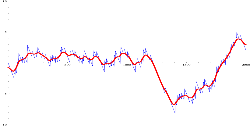
Figure 1: The least energy approximation of centered Poisson process.

For quadratic penalty the least energy approximation can be found explicitly. We study its behavior in a long run (when $T\to\infty$) and show that under weak assumption on $B$ it converges to some limit with exponential rate.

In Section 2 we provide necessary exact and asymptotic formulas for the least energy approximation of a deterministic function. In Section 3 the central results of the article related to the approximation of a random process with stationary increments are obtained. If $B$ is a random process with stationary increments, then on large intervals its least energy approximation (cf. Figure 1) also is close to a process of the same class and the relation between the corresponding spectral measures can be found. We show that in a long run (when $T\to\infty$) the expectation of energy of optimal approximation per unit of time converges to some limit. For Gaussian and Lévy processes we complete this result with almost sure and $L^{1}$ convergence. As an example, the asymptotic expression of approximation energy is found for fractional Brownian motion. In view of the importance of Wiener process, we propose an alternative approach to its least energy approximation in Section 4.

Finally, we wish to notice that our results can be considered as a complement to those of traditional stochastic control theory, where the best approximating function is chosen among the adapted ones, i.e. its value at time $t$ must be determined by the values of the target function $B(s)$, $s\leq t$. Adaptive approach is more realistic but it leads to the problems solvable mainly for Markov target processes (see e.g. [5], [6] for the least energy approximation of Wiener process). One may consider our results as the lower bounds for the least energy achievable by adaptive control in case it is unknown, or as the evaluation of price to be paid for not knowing the future, in case when both optimal adaptive and non-adaptive least energy approximations are known.

2 Least energy approximation: deterministic setting

2.1 Approximation on a fixed interval

The following variational problem (which is our starting point) and its solution are quite standard facts from variational calculus. We provide the proof for the sake of completeness but postpone it to the end of the article.

Let $B(\cdot)$ be a fixed deterministic function on an interval $[0,T]$. In this section we deal with minimization problem of the functional

$${\mathcal{E}}_{T}(f):=\int_{0}^{T}\left[f^{\prime}(t)^{2}+Q(f(t)-B(t))\right]dt$$

over the Sobolev space ${\mathbb{W}}_{2}^{1}[0,T]$ of all absolutely continuous functions $f:[0,T]\to\mathbb{R}$ having square integrable derivative. Here $Q(\cdot)$ is an appropriate penalty function.

Proposition 2.1

Let $B(\cdot)$ be a measurable function on $[0,T]$ and let $Q(\cdot)$ be a strictly convex non-negative differentiable function on $\mathbb{R}$ such that

$$\lim_{x\to\pm\infty}Q(x)=+\infty.$$

Assume that either $B$ is bounded or for some $A>0$, $p\geq 0$ it is true that $B\in L_{p+1}[0,T]$ and

$$|Q^{\prime}(x)|\leq A(|x|^{p}+1),\qquad x\in\mathbb{R}.$$ (1)

Then there exists a unique solution $f_{T}$ of the problem

$${\mathcal{E}}_{T}(f)\searrow\min,\quad f\in{\mathbb{W}}_{2}^{1}[0,T]\,.$$ (2)

This solution has absolutely continuous first derivative $f_{T}^{\prime}(\cdot)$ and satisfies the equation

$$2\,f_{T}^{\prime\prime}(t)=Q^{\prime}(f_{T}(t)-B(t)),\qquad\textrm{for a.e. }t\in(0,T),$$

and the boundary conditions $(f_{T})_{+}^{\prime}(0)=(f_{T})_{-}^{\prime}(T)=0$.

Remark 2.2

In the following we will apply this proposition to random functions $B$ that are not necessarily bounded but belong to $L_{2}[0,T]$ almost surely. Therefore, assumption (1) is adequate.

For the rest of the paper, we restrict attention to the quadratic penalty $Q(y)=y^{2}$ because in this case we are able to obtain explicit and quite meaningful results.

Proposition 2.3

Let $B\in L_{2}[0,T]$. The solution of the minimization problem with quadratic penalty

$${\mathcal{E}}_{T}(f):=\int_{0}^{T}\left[f^{\prime}(t)^{2}+|f(t)-B(t)|^{2}\right]dt\searrow\min$$

is given for $0\leq t\leq T$ by

$$f_{T}(t)=-\int_{0}^{t}B(s)\sinh(t-s)\,ds+\frac{\int_{0}^{T}B(s)\cosh(T-s)\,ds}{e^{T}-e^{-T}}\left(e^{t}+e^{-t}\right).$$ (3)

Moreover, for $0<t<T$ we have

$$f_{T}^{\prime}(t)=-\int_{0}^{t}B(s)\cosh(t-s)\,ds+\frac{\int_{0}^{T}B(s)\cosh(T-s)\,ds}{e^{T}-e^{-T}}\left(e^{t}-e^{-t}\right).$$ (4)

Proof: From Proposition 2.1 we know that the minimizer $f_{T}$ exists uniquely and solves the differential equation

$$f^{\prime\prime}(t)=f(t)-B(t)$$ (5)

with boundary conditions

$$f_{+}^{\prime}(0)=f_{-}^{\prime}(T)=0.$$

The general form of the solution for linear equation (5) without boundary conditions is

$$f(t)=f_{*}(t)+C_{1}e^{t}+C_{2}e^{-t}$$

where $f_{*}$ is any fixed solution of (5).

Let us check that

$$f_{*}(t):=-\int_{0}^{t}B(s)\sinh(t-s)ds=\frac{1}{2}\left[e^{-t}\int_{0}^{t}B(s)e^{s}ds-e^{t}\int_{0}^{t}B(s)e^{-s}ds\right]$$

indeed provides a solution of (5). We have

$$f^{\prime}_{*}(t) = \frac{1}{2}\left[-e^{-t}\int_{0}^{t}B(s)e^{s}ds+e^{-t}B(t)e^{t}-e^{t}\int_{0}^{t}B(s)e^{-s}ds-e^{t}B(t)e^{-t}\right]$$ (6)

$$= -\frac{1}{2}\left[e^{-t}\int_{0}^{t}B(s)e^{s}ds+e^{t}\int_{0}^{t}B(s)e^{-s}ds\right]$$

$$= -\int_{0}^{t}B(s)\cosh(t-s)ds.$$

It follows that

$$f^{\prime\prime}_{*}(t) = -\frac{1}{2}\left[-e^{-t}\int_{0}^{t}B(s)e^{s}ds+e^{-t}B(t)e^{t}+e^{t}\int_{0}^{t}B(s)e^{-s}ds+e^{t}B(t)e^{-t}\right]$$

$$= \frac{1}{2}\left[e^{-t}\int_{0}^{t}B(s)e^{s}ds-e^{t}\int_{0}^{t}B(s)e^{-s}ds-2B(t)\right]$$

$$= f_{*}(t)-B(t),$$

and we see that (5) holds.

Next, we adjust the coefficients $C_{1}$ and $C_{2}$ by using boundary conditions. From

$$0=f_{+}^{\prime}(0)=(f_{*})_{+}^{\prime}(0)+C_{1}-C_{2}=C_{1}-C_{2}$$

we derive $C_{1}=C_{2}$. From

$$0=f_{-}^{\prime}(T)=(f_{*})_{-}^{\prime}(T)+C_{1}\,e^{T}-C_{2}\,e^{-T}=(f_{*})_{-}^{\prime}(T)+C_{1}\,(e^{T}-e^{-T})$$

by using (6) we obtain

$$C_{1}=\frac{-(f_{*})_{-}^{\prime}(T)}{e^{T}-e^{-T}}=\frac{\int_{0}^{T}B(s)\cosh(T-s)\,ds}{e^{T}-e^{-T}}$$

and arrive at formulas (3) and (4). $\square$

2.2 Approximation in a long run

We are going now to study the behavior of the least energy approximation in a long run, i.e. when the subject of approximation, function $B(\cdot)$, is fixed while the interval length $T$ goes to infinity.

In view of future applications it will be more convenient for us to let $B(\cdot)$ be defined on the entire real line. Although approximation problem involves only the restriction of $B$ on the positive half-line, if necessary, one can always extend $B$ to the negative half-line by assigning it zero values.

Recall that the function $f_{T}(\cdot)$ defined by formula (3) provides the least energy approximation to $B(\cdot)$ on the interval $[0,T]$.

We first derive a simple approximative heuristics for $f_{T}$, then transform this heuristics into a rigorous result.

2.2.1 Heuristics

We will simplify the expressions for (3) and (4) as follows. Assume that $t,T,T-t,T-s\to+\infty$ and drop all small exponential terms $e^{-t}$, $e^{-T}$, $e^{-(T-t)}$, $e^{-(T-s)}$ where appropriate.

In particular we let

$$\frac{\cosh(T-s)}{e^{T}-e^{-T}}\left(e^{t}+e^{-t}\right) \approx \frac{1}{2}\left(e^{T-s}+e^{s-T}\right)e^{-T}e^{t}=\frac{1}{2}\left(e^{t-s}+e^{s+t-2T}\right)$$

$$= \frac{1}{2}\left(e^{t-s}+e^{s-t-2(T-t)}\right)\approx\frac{1}{2}\ e^{t-s}.$$

By plugging this into (3) and (4), we get

$$f_{T}(t) \approx \int_{0}^{t}B(s)\left(\sinh(s-t)-\frac{1}{2}\ e^{t-s}\right)ds+\int_{t}^{T}B(s)\frac{1}{2}\ e^{t-s}ds$$

$$= \frac{1}{2}\int_{0}^{t}B(s)\ e^{s-t}ds+\frac{1}{2}\int_{t}^{T}B(s)\ e^{t-s}ds$$

$$= \frac{1}{2}\int_{0}^{T}B(s)\ e^{-|s-t|}ds.$$

Similarly,

$$f_{T}^{\prime}(t)\approx\frac{1}{2}\int_{0}^{T}B(s)\operatorname{sgn}(s-t)\ e^{-|s-t|}ds.$$

Assuming that the function $B(\cdot)$ is defined on entire $\mathbb{R}$, it is more natural to use approximations based on ”stationary” kernels, i.e.  $f_{T}(t)\approx{\widehat{f}}(t)$ and $f_{T}^{\prime}(t)\approx{\widehat{f}}\,^{\prime}(t)$, where

$${\widehat{f}}(t):=\frac{1}{2}\int_{-\infty}^{\infty}B(s)\ e^{-|s-t|}ds$$ (7)

and

$${\widehat{f}}\,^{\prime}(t)=\frac{1}{2}\int_{-\infty}^{\infty}B(s)\operatorname{sgn}(s-t)\ e^{-|s-t|}ds.$$ (8)

Notice that the approximations ${\widehat{f}}$ and ${\widehat{f}}\,^{\prime}$ do not depend on $T$. This shows a local nature of the least energy approximation in a long run.

2.2.2 Rigorous result

The following result shows that the least energy approximation is exponentially close to its stationary approximation at the bulk values of time.

Proposition 2.4

Assume that

$$|B(s)|\leq C(|s|+1)^{p},\qquad s\in\mathbb{R},$$ (9)

for some $C,p>0$. Let $f_{T}$ be the least energy approximation given by (3) and let approximation ${\widehat{f}}$ be given by (7).

Then for all $T\geq 1$ and all $t\in[0,T]$ we have

$$|f_{T}(t)-{\widehat{f}}(t)|\leq C\,A_{p}\,(T+1)^{p}\left(e^{-t}+e^{-T}+e^{-(T-t)}\right),$$ (10)

and

$$|f^{\prime}_{T}(t)-{\widehat{f}}\,^{\prime}(t)|\leq C\,A_{p}\,(T+1)^{p}\left(e^{-t}+e^{-T}+e^{-(T-t)}\right),$$ (11)

where a constant $A_{p}$ depends only on $p$.

Remark 2.5

Since we are tempted by maximal generality in what concerns $B$, we will not use this proposition directly in the stochastic part of the article because of the weak but still a bit restrictive assumption (9). Instead, we will use the elements of its proof later on.

Proof of Proposition 2.4: Using the definitions (3) and (7) we see that

$$|f_{T}(t)-{\widehat{f}}(t)|\leq I_{1}+I_{2}+I_{3},$$

where

$$I_{1} = \frac{1}{2}\int_{-\infty}^{0}|B(s)|e^{-(t-s)}\,ds,$$

$$I_{2} = \int_{0}^{T}|B(s)|\,\left|K_{T}(s,t)-e^{t-s}/2\right|\,ds,$$

$$I_{3} = \frac{1}{2}\int_{T}^{\infty}|B(s)|e^{-(s-t)}\,ds,$$

and

$$K_{T}(s,t) := \frac{\cosh(T-s)}{e^{T}-e^{-T}}\left(e^{t}+e^{-t}\right)$$

$$= \frac{e^{t-s}}{2}\,\left(1+e^{-2(T-s)}\right)\left(1+e^{-2t}\right)\left(1-e^{-2T}\right)^{-1}.$$

By (9) we have

$$I_{1}\leq\frac{Ce^{-t}}{2}\int_{-\infty}^{0}(|s|+1)^{p}\,e^{s}\,ds:=C\,A_{p}^{(1)}\,e^{-t}$$

and

$$I_{3} \leq \frac{Ce^{-(T-t)}}{2}\int_{T}^{\infty}(s+1)^{p}e^{-(s-T)}\,ds$$

$$= \frac{Ce^{-(T-t)}}{2}\int_{0}^{\infty}(T+1+u)^{p}\,e^{-u}\,du$$

$$\leq \frac{C2^{p}e^{-(T-t)}}{2}\int_{0}^{\infty}((T+1)^{p}+u^{p})\,e^{-u}\,du$$

$$\leq C\,A_{p}^{(2)}(T+1)^{p}\ e^{-(T-t)}.$$

In order to evaluate $I_{2}$, notice that

$$K_{T}(s,t)-\frac{e^{t-s}}{2}=\frac{e^{t-s}}{2}\left[(1+h_{1})(1+h_{2})(1-h_{3})^{-1}-1\right]$$

where $h_{1}:=e^{-2(T-s)}$, $h_{2}:=e^{-2t}$, $h_{3}:=e^{-2T}$. Notice that assumption $T\geq 1$ yields $0\leq h_{3}\leq\tfrac{1}{2}$  . Therefore, we have

$$(1-h_{3})^{-1}=1+\frac{h_{3}}{1-h_{3}}\leq 1+2h_{3}.$$

Furthermore, inequalities $0\leq h_{1}\leq 1$, $0\leq h_{2}\leq 1$, $0\leq h_{3}\leq\tfrac{1}{2}$ yield

$$(1+h_{1})(1+h_{2})(1+2h_{3})\leq 1+4h_{1}+2h_{2}+2h_{3}.$$

We infer that

$$0 \leq K_{T}(s,t)-\frac{e^{t-s}}{2}$$ (12)

$$\leq \frac{e^{t-s}}{2}\left(4h_{1}+2h_{2}+2h_{3}\right)$$

$$\leq 2\,e^{t-s}\left(e^{-2(T-s)}+e^{-2t}+e^{-2T}\right)$$

$$= 2\left(e^{-2T+t+s}+e^{-t-s}+e^{t-s-2T}\right).$$

It follows that

$$I_{2}\leq 2\left(I_{5}+I_{6}+I_{7}\right),$$

where

$$I_{5} := C\,e^{-2T+t}\int_{0}^{T}(s+1)^{p}e^{s}\,ds\leq Ce^{-(T-t)}(T+1)^{p},$$

$$I_{6} := C\,e^{-t}\int_{0}^{T}(s+1)^{p}\,e^{-s}\,ds\leq C\,A_{p}^{(3)}\,e^{-t},\qquad A_{p}^{(3)}=e\,\Gamma(p+1),$$

$$I_{7} := C\,e^{t-2T}\int_{0}^{T}(s+1)^{p}\,e^{-s}\,ds\leq C\,A_{p}^{(3)}\,e^{-(T-t)}.$$

By combining all estimates we obtain (10).

The proof of (11) is completely similar. One should use the function

$${\widehat{K}}_{T}(s,t):=\frac{\cosh(T-s)}{e^{T}-e^{-T}}\left(e^{t}-e^{-t}\right)$$

instead of $K_{T}(s,t)$. Then (12) is replaced by

$$-e^{-t-s}\leq{\widehat{K}}_{T}(s,t)-\frac{e^{t-s}}{2}\leq\left(e^{-2T+t+s}+e^{t-s-2T}\right),$$ (13)

and all calculations go in the same way. $\square$

Once the proposition is proved, we have straightforward integral estimates. Let $||\cdot||_{2,T}$ denote the norm in the space $L_{2}[0,T]$.

Corollary 2.6

Under assumptions of Proposition 2.1, we have

$$\|f_{T}-{\widehat{f}}\|_{2,T}\leq 2\,C\,A_{p}\,(T+1)^{p}$$

and

$$\|f^{\prime}_{T}-{\widehat{f}}\,^{\prime}\|_{2,T}\leq 2\,C\,A_{p}\,(T+1)^{p}.$$ (14)

Proof: We have

$$\|f_{T}-{\widehat{f}}\|_{2,T}^{2} = \int_{0}^{T}\|f_{T}(t)-{\widehat{f}}(t)|^{2}dt$$

$$\leq C^{2}\,A_{p}^{2}\,(T+1)^{2p}\int_{0}^{T}\left(e^{-t}+e^{-T}+e^{-(T-t)}\right)^{2}dt$$

$$\leq 3\,C^{2}\,A_{p}^{2}\,(T+1)^{2p}\int_{0}^{T}\left(e^{-2t}+e^{-2T}+e^{-2(T-t)}\right)dt$$

$$\leq 3\,C^{2}\,A_{p}^{2}\,(T+1)^{2p}\left(\frac{1}{2}+Te^{-2T}+\frac{1}{2}\right)$$

$$\leq 4\,C^{2}\,A_{p}^{2}\,(T+1)^{2p},$$

where at the last step we used assumption $T\geq 1$.

The proof of (14) is completely similar. $\square$

3 Application to processes with stationary increments

3.1 A brief reminder on the processes with stationary increments

A complex-valued random process $B(t),t\in\mathbb{R}$, is called process with stationary increments in the wide sense if it has finite second moments and the mean and the covariance of the process $B_{t_{0}}(t):=B(t_{0}+t)-B(t_{0})$ are the same for all $t_{0}\in\mathbb{R}$. If such process is stochastically continuous, then it admits a spectral representation of the form

$$B(t)=B_{0}+D_{0}t+\int_{\mathbb{R}\backslash\{0\}}(e^{itu}-1)X(du),$$ (15)

where $B_{0},D_{0}$ are random variables with finite second moment and $X(du)$ is a complex-valued zero mean uncorrelated random measure on $\mathbb{R}\backslash\{0\}$, uncorrelated with $D_{0}$, see [14]. In the following we assume $B_{0}=0$ since the initial value is irrelevant to our purposes.

Recall that the covariance structure of $B$ is characterized by a deterministic spectral measure $\mu_{B}$ on $\mathbb{R}\backslash\{0\}$ defined by $\mu_{B}(A):=\mathbb{E}\,|X(A)|^{2}$. The spectral measure may be infinite but it must satisfy Lévy’s integrability condition

$$\int_{\mathbb{R}\backslash\{0\}}\min(u^{2},1)\mu_{B}(du)<\infty.$$

In the sequel, $B(t),t\in\mathbb{R}$, denotes a stochastically continuous, real-valued process with stationary increments in the wide sense such that $B(0)=0$. We always work with a measurable version of $B$. Let us stress that even though $B$ is a real-valued process, the random measure $X$ may be complex, yet it must satisfy condition $X(-A)=\overline{X(A)}$.

The standard deviation of $B$ grows at most linearly. We will use the following estimate:

$$\mathbb{E}\,|B(t)|^{2} = \mathbb{E}\,|D_{0}|^{2}t^{2}+\int_{\mathbb{R}\backslash\{0\}}|e^{itu}-1|^{2}\mu_{B}(du)$$

$$\leq \mathbb{E}\,|D_{0}|^{2}t^{2}+\int_{-1}^{1}u^{2}\mu_{B}(du)t^{2}+4\mu_{B}\{\mathbb{R}\backslash[-1,1]\}$$

$$\leq A(t^{2}+1),$$

where

$$A:=\max\left\{\mathbb{E}\,|D_{0}|^{2}+\int_{-1}^{1}u^{2}\mu_{B}(du),4\mu_{B}\{\mathbb{R}\backslash[-1,1]\}\right\}.$$

It follows that for any $T>0$

$$\mathbb{E}\,\int_{0}^{T}|B(t)|^{2}dt<\infty,$$

therefore $B\in L_{2}[0,T]$ almost surely, and Proposition 2.1 applies to the sample paths of $B$ with $p=1$.

If we additionally assume that the random measure $X$ is Gaussian, then the process $B$ is also Gaussian. Fractional Brownian motions $W^{(H)}(t)$, $0<H\leq 1$, are the most known Gaussian processes with stationary increments. The range of parameter $0<H<1$ is associated to the family of spectral measures

$$\mu_{H}(du):=\frac{M_{H}\,du}{|u|^{2H+1}}\,,\qquad M_{H}:=\frac{\Gamma(2H+1)\sin(\pi H)}{2\pi}\,,$$

with $D_{0}=0$. We have a power-type variance

$$\mathbb{E}\,|W^{(H)}(t)|^{2} = \int_{-\infty}^{\infty}|e^{itu}-1|^{2}\frac{M_{H}\,du}{|u|^{2H+1}}$$

$$= 2\int_{-\infty}^{\infty}(1-\cos(tu))\,\frac{M_{H}\,du}{|u|^{2H+1}}$$

$$= 4M_{H}\,|t|^{2H}\int_{0}^{\infty}(1-\cos v)\,\frac{dv}{v^{2H+1}}$$

$$= 4M_{H}\,|t|^{2H}(2H)^{-1}\int_{0}^{\infty}\sin v\,\frac{dv}{v^{2H}}$$

$$= 4M_{H}\,|t|^{2H}(2H)^{-1}\ \frac{\pi}{2\Gamma(2H)\sin(\pi H)}$$

$$= |t|^{2H}.$$

The case $H=1$ is degenerate linear, i.e. $W^{(1)}(t)=D_{0}t$ with $D_{0}$ being a standard Gaussian random variable. The remarkable properties of fractional Brownian motions are described e.g. in [11, Section 7.2] and in [3, Chapter 4].

Wiener process $W$ is a special case of fractional Brownian motion corresponding to $H=\tfrac{1}{2}$. It has a spectral measure $\mu_{W}(du)=\tfrac{du}{2\pi|u|^{2}}$.

3.2 Convergence of average least energy

The following result describes the behavior of the average least energy approximation for arbitrary process with (wide-sense) stationary increments. We call

$${\mathcal{E}}_{T}(f,B):=\int_{0}^{T}\left[(f(s)-B(s))^{2}+f^{\prime}(s)^{2}\right]ds$$

the energy of function $f$ with respect to $B$ on the interval $[0,T]$. If the function $B$ is fixed, we omit it from the notation.

Theorem 3.1

Let $B(t),t\in\mathbb{R}$, be a stochastically continuous process with wide-sense stationary increments given by its spectral representation (15). Recall that $f_{T}$ denotes the minimizer of ${\mathcal{E}}_{T}(f,B)$ over all $f\in{\mathbb{W}}_{2}^{1}[0,T]$. Then,

$$\lim_{T\to\infty}T^{-1}\mathbb{E}\,{\mathcal{E}}_{T}(f_{T},B)={\mathcal{C}},$$ (16)

where

$${\mathcal{C}}:=\mathbb{E}\,|D_{0}|^{2}+\int_{\mathbb{R}\backslash\{0\}}\frac{u^{2}}{1+u^{2}}\ \mu_{B}(du).$$ (17)

The constant ${\mathcal{C}}$ means the smallest average amount of energy per unit of time needed for approximation of $B$.

Corollary 3.2

For the fractional Brownian motion we have

$${\mathcal{C}} = \int_{\mathbb{R}\backslash\{0\}}\frac{u^{2}}{1+u^{2}}\ \frac{M_{H}du}{|u|^{2H+1}}=2M_{H}\int_{0}^{\infty}\ \frac{u^{1-2H}\,du}{1+u^{2}}$$

$$= M_{H}\int_{0}^{\infty}\ \frac{v^{-H}\,dv}{1+v}$$

$$= M_{H}\cdot\frac{\pi}{\sin(\pi H)}=\frac{\Gamma(2H+1)}{2}.$$

For the Wiener process $H=\tfrac{1}{2}$ this yields the constant

$${\mathcal{C}}=\frac{1}{2}$$ (18)

that can be also obtained by other method (see Section 4 below).

Remark 3.3

We can give an alternative non-spectral representation for the constant ${\mathcal{C}}$, namely,

$${\mathcal{C}}=(\mathbb{E}\,\,D_{0})^{2}+\frac{1}{2}\int_{0}^{\infty}\operatorname{Var}(B(s))\,e^{-s}ds.$$

Indeed,

$$(\mathbb{E}\,D_{0})^{2}+\frac{1}{2}\int_{0}^{\infty}\operatorname{Var}(B(s))\,e^{-s}ds$$

$$= (\mathbb{E}\,D_{0})^{2}+\frac{1}{2}\int_{0}^{\infty}\operatorname{Var}(D_{0})\,s^{2}e^{-s}ds$$

$$+\frac{1}{2}\int_{0}^{\infty}\left(\int_{\mathbb{R}\backslash\{0\}}|1-e^{isu}|^{2}\ \mu_{B}(du)\right)e^{-s}ds$$

$$= \mathbb{E}\,D_{0}^{2}+\frac{1}{2}\int_{\mathbb{R}\backslash\{0\}}\left(\int_{0}^{\infty}(2-e^{isu}-e^{isu})\,e^{-s}ds\right)\mu_{B}(du)$$

$$= \mathbb{E}\,D_{0}^{2}+\frac{1}{2}\int_{\mathbb{R}\backslash\{0\}}\left(2-\frac{1}{1-iu}-\frac{1}{1+iu}\right)\mu_{B}(du)$$

$$= \mathbb{E}\,D_{0}^{2}+\int_{\mathbb{R}\backslash\{0\}}\frac{u^{2}}{1+u^{2}}\ \mu_{B}(du)={\mathcal{C}}.$$

Remark 3.4

Would we introduce a viscosity constant $\kappa>0$, i.e. change the penalty to $Q(y)=\kappa^{2}y^{2}$, by a linear time change the minimal energy approximation problem on $[0,T]$ for $B$ reduces to that for the process $\widetilde{B}(t):=B(t/\kappa)$ on the interval $[0,\kappa T]$ with $\kappa=1$. Thus the limit energy constant from (17) becomes

$${\mathcal{C}}_{\kappa}:=\mathbb{E}\,|D_{0}|^{2}+\int_{\mathbb{R}\backslash\{0\}}\frac{\kappa^{2}u^{2}}{\kappa^{2}+u^{2}}\ \mu_{B}(du)$$

in this case.

Remark 3.5

It is worthwhile to compare the least energy approximation constant for Wiener process (18) with analogous result of adaptive control, see [5, p.319]. It turns out that the optimal adaptive control requires two times more energy than the non-adaptive one.

Proof of Theorem 3.1: Consider approximations (7) and (8) related to $B$. They become

$${\widehat{f}}(t) = D_{0}t+\frac{1}{2}\int_{-\infty}^{\infty}\int_{\mathbb{R}\backslash\{0\}}\ e^{-|s-t|}\left(e^{isu}-1\right)X(du)\,ds$$

$$:= D_{0}t+\int_{\mathbb{R}\backslash\{0\}}K^{(0)}(t,u)X(du)$$

and

$${\widehat{f}}\,^{\prime}(t) = D_{0}+\frac{1}{2}\int_{-\infty}^{\infty}\int_{\mathbb{R}\backslash\{0\}}\operatorname{sgn}(s-t)\ e^{-|s-t|}\left(e^{isu}-1\right)X(du)\,ds$$

$$:= D_{0}+\int_{\mathbb{R}\backslash\{0\}}K^{(1)}(t,u)X(du),$$

where we have expressions for respective kernels

$$K^{(0)}(t,u) = \frac{1}{2}\,\int_{-\infty}^{\infty}\ e^{-|s-t|}\left(e^{isu}-1\right)ds$$

$$= \frac{1}{2}\ e^{itu}\int_{-\infty}^{\infty}\ e^{-|v|}e^{ivu}dv-1$$

$$= \frac{1}{2}\ e^{itu}\left(\int_{-\infty}^{0}\ e^{(1+iu)v}dv+\int_{0}^{\infty}\ e^{-(1-iu)v}dv\right)-1$$

$$= \frac{1}{2}\ e^{itu}\left(\frac{1}{1+iu}+\frac{1}{1-iu}\right)-1$$

$$= \frac{e^{itu}}{1+u^{2}}-1,$$

and

$$K^{(1)}(t,u) = \frac{1}{2}\int_{-\infty}^{\infty}\ \operatorname{sgn}(s-t)\,e^{-|s-t|}\,\left(e^{isu}-1\right)\,ds$$

$$= \frac{1}{2}\ e^{itu}\int_{-\infty}^{\infty}\ \operatorname{sgn}(v)\,e^{-|v|}\,e^{ivu}\,dv$$

$$= \frac{1}{2}\ e^{itu}\left(-\int_{-\infty}^{0}\ e^{(1+iu)v}dv+\int_{0}^{\infty}\ e^{-(1-iu)v}\,dv\right)$$

$$= \frac{1}{2}\ e^{itu}\left(-\frac{1}{1+iu}+\frac{1}{1-iu}\right)$$

$$= \frac{iu\,e^{itu}}{1+u^{2}}\ .$$

We conclude that

$${\widehat{f}}(t)-B(t)=\int_{\mathbb{R}\backslash\{0\}}\left(\frac{1}{1+u^{2}}-1\right)\,e^{itu}\,X(du)=\int_{\mathbb{R}\backslash\{0\}}\frac{-u^{2}}{1+u^{2}}\ e^{itu}\,X(du)$$

and

$${\widehat{f}}\,^{\prime}(t)=D_{0}+\int_{\mathbb{R}\backslash\{0\}}\frac{iu}{1+u^{2}}\ e^{itu}\,X(du).$$ (19)

We see that both deviation ${\widehat{f}}-B$ and derivative ${\widehat{f}}\,^{\prime}$ are wide sense stationary processes. By the well known isometric property we have

$$\mathbb{E}\,|{\widehat{f}}(t)-B(t)|^{2}=\int_{\mathbb{R}\backslash\{0\}}\frac{u^{4}}{(1+u^{2})^{2}}\ \mu_{B}(du),\qquad t\in\mathbb{R},$$

and

$$\mathbb{E}\,|{\widehat{f}}\,^{\prime}(t)|^{2}=\mathbb{E}\,|D_{0}|^{2}+\int_{\mathbb{R}\backslash\{0\}}\frac{u^{2}}{(1+u^{2})^{2}}\ \mu_{B}(du),\qquad t\in\mathbb{R}.$$

Hence, for any $T>0$ we have

$$\mathbb{E}\,{\mathcal{E}}_{T}({\widehat{f}},B) = \int_{0}^{T}\left[\mathbb{E}\,|{\widehat{f}}(t)-B(t)|^{2}+\mathbb{E}\,|{\widehat{f}}\,^{\prime}(t)|^{2}\right]dt$$

$$= T\left[\mathbb{E}\,|{\widehat{f}}(0)-B(0)|^{2}+\mathbb{E}\,|{\widehat{f}}\,^{\prime}(0)|^{2}\right]$$

$$= T\left[\mathbb{E}\,|D_{0}|^{2}+\int_{\mathbb{R}\backslash\{0\}}\frac{u^{4}+u^{2}}{(1+u^{2})^{2}}\ \mu_{B}(du)\right]$$

$$= T\left[\mathbb{E}\,|D_{0}|^{2}+\int_{\mathbb{R}\backslash\{0\}}\frac{u^{2}}{1+u^{2}}\ \mu_{B}(du)\right].$$

$$= T\,{\mathcal{C}}.$$

It remains to show that the average energy of the least energy approximation $f_{T}$ and that of stationary approximation ${\widehat{f}}$ are sufficiently close, i.e.

$$\lim_{T\to\infty}T^{-1}[\mathbb{E}\,{\mathcal{E}}_{T}(f_{T},B)-\mathbb{E}\,{\mathcal{E}}_{T}({\widehat{f}},B)]=0.$$ (20)

Notice that by triangle inequality in $L_{2}[0,1]$ we have

$$\left|\sqrt{{\mathcal{E}}_{T}(f_{T},B)}-\sqrt{{\mathcal{E}}_{T}({\widehat{f}},B)}\right|\leq\sqrt{{\mathcal{E}}_{T}(f_{T}-{\widehat{f}},0)},$$

hence,

$$\left|{\mathcal{E}}_{T}(f_{T},B)-{\mathcal{E}}_{T}({\widehat{f}},B)\right|\leq{\mathcal{E}}_{T}(f_{T}-{\widehat{f}},0)+2\sqrt{{\mathcal{E}}_{T}({\widehat{f}},B)}\ \sqrt{{\mathcal{E}}_{T}(f_{T}-{\widehat{f}},0)}$$

and

$$\left|\mathbb{E}\,{\mathcal{E}}_{T}(f_{T},B)-\mathbb{E}\,{\mathcal{E}}_{T}({\widehat{f}},B)\right|\leq\mathbb{E}\,\left|{\mathcal{E}}_{T}(f_{T},B)-{\mathcal{E}}_{T}({\widehat{f}},B)\right|$$ (21)

$$\leq \mathbb{E}\,{\mathcal{E}}_{T}(f_{T}-{\widehat{f}},0)+2\,\mathbb{E}\,\left(\sqrt{{\mathcal{E}}_{T}({\widehat{f}},B)}\ \sqrt{{\mathcal{E}}_{T}(f_{T}-{\widehat{f}},0)}\right)$$

$$\leq \mathbb{E}\,{\mathcal{E}}_{T}(f_{T}-{\widehat{f}},0)+2\,\sqrt{\mathbb{E}\,{\mathcal{E}}_{T}({\widehat{f}},B)\ \mathbb{E}\,{\mathcal{E}}_{T}(f_{T}-{\widehat{f}},0)}$$

$$= \mathbb{E}\,{\mathcal{E}}_{T}(f_{T}-{\widehat{f}},0)+2\,\sqrt{{\mathcal{C}}T\,{\mathcal{E}}_{T}(f_{T}-{\widehat{f}},0)}.$$

We see that

$$\lim_{T\to\infty}T^{-1}[\mathbb{E}\,{\mathcal{E}}_{T}(f_{T}-{\widehat{f}},0)]=0$$ (22)

would imply the desired relation (20).

We first analyze the potential energy and prove that

$$\sup_{T>0}\sup_{0\leq t\leq T}\mathbb{E}\,|f_{T}(t)-B(t)|^{2}<\infty,$$ (23)

$$\sup_{t\geq 0}\mathbb{E}\,|{\widehat{f}}(t)-B(t)|^{2}<\infty.$$ (24)

The part concerning ${\widehat{f}}$ is trivial because ${\widehat{f}}-B$ is stationary. Furthermore, let us represent

$$f_{T}(t)-B(t)=\int_{0}^{T}R_{T}(s,t)(B(s)-B(t))ds$$

where for $s\in[t,T]$ we have by (12)

$$0 \leq R_{T}(s,t):=K_{T}(s,t)$$

$$\leq \frac{e^{t-s}}{2}+2\left(e^{-2T+t+s}+e^{-t-s}+e^{t-s-2T}\right)$$

$$= \frac{e^{t-s}}{2}+2\left(e^{(t-s)+2(s-T)}+e^{(t-s)-2t}+e^{(t-s)-2T}\right)$$

$$\leq 7e^{t-s}=7e^{-|t-s|},$$

while for $s\in[0,t]$ we have

$$0 \leq R_{T}(s,t):=K_{T}(s,t)-\sinh(t-s)$$

$$= \left(K_{T}(s,t)-\frac{e^{t-s}}{2}\right)+\frac{e^{s-t}}{2}$$

$$\leq \ \left(e^{-2T+t+s}+e^{-t-s}+e^{t-s-2T}\right)+\frac{e^{s-t}}{2}$$

$$= \ \left(e^{(s-t)-2(T-t)}+e^{(s-t)-2s}+e^{(s-t)-2(T-(t-s))}\right)+\frac{e^{s-t}}{2}$$

$$\leq 7e^{s-t}=7e^{-|t-s|}.$$

Hence,

$$\mathbb{E}\,|f_{T}(t)-B(t)|^{2} \leq \mathbb{E}\,\left(7\int_{0}^{T}e^{-|t-s|}|B(s)-B(t)|ds\right)^{2}$$

$$\leq c\,\mathbb{E}\,\int_{0}^{T}e^{-|t-s|}|B(s)-B(t)|^{2}ds$$

$$\leq c\,A\int_{0}^{T}e^{-|t-s|}[(s-t)^{2}+1]ds$$

and (23) follows. By using also (24) we obtain

$$\sup_{T>0}\sup_{0\leq t\leq T}\mathbb{E}\,|f_{T}(t)-{\widehat{f}}(t)|^{2}<\infty.$$ (25)

This estimate is still too crude, and we continue as follows.

$$f_{T}(t)-{\widehat{f}}(t) = -\int_{-\infty}^{0}e^{-(t-s)}B(s)ds$$

$$+\int_{0}^{T}(K_{T}(s,t)-e^{t-s}/2)B(s)ds-\int_{T}^{\infty}e^{-(s-t)}B(s)ds$$

$$:= G_{1}(t)+G_{2}(t)+G_{3}(t).$$

For $G_{1}$ we have

$$\mathbb{E}\,|G_{1}(t)|^{2} \leq e^{-2t}\,\mathbb{E}\,\left(\int_{-\infty}^{0}e^{s}|B(s)|ds\right)^{2}$$

$$\leq e^{-2t}\,\mathbb{E}\,\left(\int_{-\infty}^{0}e^{s}|B(s)|^{2}ds\right)$$

$$\leq e^{-2t}A\int_{-\infty}^{0}e^{s}(|s|^{2}+1)ds:=c\,e^{-2t}.$$

For $G_{3}$ we have

$$\mathbb{E}\,|G_{3}(t)|^{2} \leq e^{-2(T-t)}\mathbb{E}\,\left(\int_{T}^{\infty}e^{T-s}|B(s)|\,ds\right)^{2}$$

$$\leq e^{-2(T-t)}\mathbb{E}\,\left(\int_{T}^{\infty}e^{T-s}|B(s)|^{2}\,ds\right)$$

$$\leq e^{-2(T-t)}A\int_{T}^{\infty}e^{T-s}(s^{2}+1)\,ds$$

$$\leq e^{-2(T-t)}A\int_{T}^{\infty}e^{T-s}(2(s-T)^{2}+2T^{2}+1)\,ds$$

$$\leq cA(T^{2}+1)\,e^{-2(T-t)}.$$

This estimate is not good enough when $t$ is close to $T$. This is why we need (25). For $G_{2}$ we have by (12)

$$|G_{2}(t)|\leq 2(G_{2,1}(t)+G_{2,2}(t)+G_{2,3}(t)),$$

where

$$G_{2,1}(t) = \int_{0}^{T}e^{t-2T+s}|B(s)|ds,$$

$$G_{2,2}(t) = \int_{0}^{T}e^{-t-s}|B(s)|ds,$$

$$G_{2,3}(t) = \int_{0}^{T}e^{t-s-2T}|B(s)|ds.$$

Moreover,

$$\mathbb{E}\,|G_{2,1}(t)|^{2} = e^{2t-4T}\mathbb{E}\,\left(\int_{0}^{T}e^{s}|B(s)|ds\right)^{2}$$

$$\leq e^{2t-4T}\mathbb{E}\,\left(e^{T}\int_{0}^{T}e^{s}|B(s)|^{2}ds\right)$$

$$\leq e^{2t-3T}A\int_{0}^{T}e^{s}(s^{2}+1)ds$$

$$\leq 2A\,e^{-2(T-t)}(T^{2}+1),$$

$$\mathbb{E}\,|G_{2,2}(t)|^{2} = e^{-2t}\mathbb{E}\,\left(\int_{0}^{T}e^{-s}|B(s)|ds\right)^{2}$$

$$\leq e^{-2t}\mathbb{E}\,\left(\int_{0}^{T}e^{-s}|B(s)|^{2}ds\right)$$

$$\leq e^{-2t}A\int_{0}^{T}e^{-s}(s^{2}+1)ds$$

$$\leq 3A\,e^{-2t},$$

$$\mathbb{E}\,|G_{2,3}(t)|^{2} = e^{2t-4T}\mathbb{E}\,\left(\int_{0}^{T}e^{-s}|B(s)|ds\right)^{2}$$

$$\leq e^{2t-4T}\mathbb{E}\,\left(\int_{0}^{T}e^{-s}|B(s)|^{2}ds\right)$$

$$\leq e^{2t-4T}\int_{0}^{T}e^{-s}(s^{2}+1)ds$$

$$\leq 3Ae^{-2(T-t)}.$$

We summarize the latter calculations as

$$\mathbb{E}\,|f_{T}(t)-{\widehat{f}}(t)|^{2}\leq cA\left(e^{-2t}+e^{-2(T-t)}(T^{2}+1)\right).$$ (26)

Now we proceed with integration over $[0,T]$. By applying (26) on the interval $[0,T-3\ln T]$ and (25) on the interval $[T-3\ln T,T]$ we obtain

$$\mathbb{E}\,\int_{0}^{T}|f_{T}(t)-{\widehat{f}}(t)|^{2}dt\leq cA(1+\ln T)=o(T).$$ (27)

Kinetic energy is studied in the same fashion. By using (13) instead of (12), we replace (23), (24) with

$$\sup_{T>0}\sup_{0\leq t\leq T}\mathbb{E}\,|f^{\prime}_{T}(t)|^{2}<\infty,$$

$$\sup_{t\geq 0}\mathbb{E}\,|{\widehat{f}}\,^{\prime}(t)|^{2}<\infty.$$

Hence may be (25) replaced by

$$\sup_{T>0}\sup_{0\leq t\leq T}\mathbb{E}\,|f_{T}(t)-{\widehat{f}}(t)|^{2}<\infty.$$

Further, using again (13) we replace (26) with

$$\mathbb{E}\,|f^{\prime}_{T}(t)-{\widehat{f}}\,^{\prime}(t)|^{2}\leq cA\left(e^{-2t}+e^{-2(T-t)}(T^{2}+1)\right).$$

Integration yields

$$\mathbb{E}\,\int_{0}^{T}|f^{\prime}_{T}(t)-{\widehat{f}}\,^{\prime}(t)|^{2}dt\leq cA(1+\ln T).$$ (28)

By merging (27) and (28) we get

$$\mathbb{E}\,{\mathcal{E}}_{T}(f_{T}-{\widehat{f}},0)\leq cA(1+\ln T),$$ (29)

which is a quantitative version of the remaining relation (22). $\square$

3.3 Almost sure and $L_{1}$ convergence

The random variable

$$Z := |D_{0}|^{2}-\mathbb{E}\,|D_{0}|^{2}+{\mathcal{C}}$$

$$= |D_{0}|^{2}+\int_{\mathbb{R}\backslash\{0\}}\frac{u^{2}}{1+u^{2}}\,\mu_{B}(du)$$

is a right candidate for the a.s. least energy limit. Notice that if $B$ has no systematic drift (i.e. $D_{0}=0$), then $Z={\mathcal{C}}$ is a deterministic constant.

We first develop a reduction tool showing that almost sure and $L_{1}$ convergence of the least approximation energy are reduced to the stationary case.

Proposition 3.6

If $T^{-1}{\mathcal{E}}_{T}({\widehat{f}},B)\ {\buildrel\hbox{\scriptsize a.s. }\over{\to}}\ Z$, then $T^{-1}{\mathcal{E}}_{T}(f_{T},B)\ {\buildrel\hbox{\scriptsize a.s. }\over{\to}}\ Z$.

If $T^{-1}{\mathcal{E}}_{T}({\widehat{f}},B)\ {\buildrel L_{1}\over{\to}}\ Z$, then $T^{-1}{\mathcal{E}}_{T}(f_{T},B)\ {\buildrel L_{1}\over{\to}}\ Z$.

Proof: We know from (21) and (29) that for any $T$

$$\mathbb{E}\,\left|{\mathcal{E}}_{T}(f_{T},B)-{\mathcal{E}}_{T}({\widehat{f}},B)\right|\leq cA\sqrt{T(1+\ln T)}.$$ (30)

Let us fix any $a>1$ and consider geometric sequence of times $T_{n}:=a^{n}$. It follows from (30) that

$$\mathbb{E}\,\sum_{n=1}^{\infty}T_{n}^{-1}\left|{\mathcal{E}}_{T_{n}}(f_{T_{n}},B)-{\mathcal{E}}_{T_{n}}({\widehat{f}},B)\right|<\infty.$$

Therefore,

$$T_{n}^{-1}\left|{\mathcal{E}}_{T_{n}}(f_{T_{n}},B)-{\mathcal{E}}_{T_{n}}({\widehat{f}},B)\right|\to 0$$

almost surely and in $L_{1}$. Under assumptions of our proposition we obtain

$$T_{n}^{-1}{\mathcal{E}}_{T_{n}}(f_{T_{n}},B)\to Z$$

almost surely (resp. in $L_{1}$).

Furthermore, since the least approximation energy ${\mathcal{E}}_{T}(f_{T},B)$ is an increasing function of $T$, we have for any $T\in[T_{n},T_{n+1}]$

$$\left|T^{-1}{\mathcal{E}}_{T}(f_{T},B)-Z\right|$$

$$\leq \max\left\{\left|T^{-1}{\mathcal{E}}_{T_{n}}(f_{T_{n}},B)-Z\right|,\left|T^{-1}{\mathcal{E}}_{T_{n+1}}(f_{T_{n+1}},B)-Z\right|\right\}$$

$$\leq a\max\left\{\left|T_{n}^{-1}{\mathcal{E}}_{T_{n}}(f_{T_{n}},B)-Z\right|,\left|T_{n+1}^{-1}{\mathcal{E}}_{T_{n+1}}(f_{T_{n+1}},B)-Z\right|\right\}+(a-1)Z.$$

Now the a.s. convergence (resp. $L_{1}$-convergence) of $T^{-1}{\mathcal{E}}_{T}(f_{T},B)$ to $Z$ follows from that of $T_{n}^{-1}{\mathcal{E}}_{T_{n}}(f_{T_{n}},B)$ by letting $a\searrow 1$. $\square$

Proposition 3.7

If the process $B$ is Gaussian and its spectral measure $\mu_{B}$ has no atoms, then $T^{-1}{\mathcal{E}}_{T}(f_{T},B)\to Z$ in $L_{1}$ and almost surely, as $T\to\infty$.

Proof: According to Proposition 3.6, it is sufficient to prove that

$$T^{-1}{\mathcal{E}}_{T}({\widehat{f}},B)\to Z,\qquad\textrm{as }T\to\infty,$$

in $L_{1}$ and almost surely. We may split the energy into potential and kinetic parts and check that

$$T^{-1}\int_{0}^{T}|{\widehat{f}}(t)-B(t)|^{2}dt\to\int_{\mathbb{R}\backslash\{0\}}\frac{u^{4}}{(1+u^{2})^{2}}\ \mu_{B}(du)$$

and

$$T^{-1}\int_{0}^{T}|{\widehat{f}}\,^{\prime}(t)|^{2}dt\to|D_{0}|^{2}+\int_{\mathbb{R}\backslash\{0\}}\frac{u^{2}}{(1+u^{2})^{2}}\ \mu_{B}(du).$$

Recall that by (19) we have a representation

$${\widehat{f}}\,^{\prime}(t)=D_{0}+Y(t),$$

where $Y$ is a centered stationary Gaussian process with the spectral measure

$$\nu(du)=\frac{u^{2}}{(1+u^{2})^{2}}\,\mu_{B}(du).$$

It follows that

$$T^{-1}\int_{0}^{T}|{\widehat{f}}\,^{\prime}(t)|^{2}dt=|D_{0}|^{2}+2T^{-1}D_{0}\int_{0}^{T}Y(t)dt+T^{-1}\int_{0}^{T}|Y(t)|^{2}dt.$$

Recall that Gaussian stationary processes whose spectral measure has no atoms are ergodic, see [4], [8]. Since both $B(t)-{\widehat{f}}(t)$ and $Y(t)$ belong to this class, we may use Birkhoff ergodic theorem and obtain convergence of time-averages to the corresponding expectations in any $L_{p}$, $p\in(1,\infty)$, and almost surely, i.e.

$$T^{-1}\int_{0}^{T}|{\widehat{f}}(t)-B(t)|^{2}dt \to \int_{\mathbb{R}\backslash\{0\}}\frac{u^{4}}{(1+u^{2})^{2}}\ \mu_{B}(du),$$

$$T^{-1}\int_{0}^{T}Y(t)dt \to 0,$$

$$T^{-1}\int_{0}^{T}|Y(t)|^{2}dt \to \int_{\mathbb{R}\backslash\{0\}}\frac{u^{2}}{(1+u^{2})^{2}}\ \mu_{B}(du),$$

and we are done. $\square$

Another interesting class of examples where we can provide an affirmative answer for the least energy convergence is given by Lévy processes (i.e. processes with independent stationary increments).

Proposition 3.8

Let $B(t),t\geq 0$, be Lévy process having finite second moments. Then $T^{-1}{\mathcal{E}}_{T}(f_{T},B)\ {\buildrel L_{1}\over{\to}}\ Z$, and $T^{-1}{\mathcal{E}}_{T}(f_{T},B)\ {\buildrel\hbox{\scriptsize a.s. }\over{\to}}\ Z$, as $T\to\infty$, where

$$Z={\mathcal{C}}=|\mathbb{E}\,B(1)|^{2}+\frac{\operatorname{Var}B(1)}{2}.$$

Proof: Without loss of generality, we may extend $B$ to the negative half-axis in such a way that $-B(-t),t\leq 0$, is an independent equidistributed copy of $B(t),t\geq 0$. Looking at $B$ as a process with stationary increments in the wide sense, we see that its linear part $D_{0}t$ is deterministic, and $\mathbb{E}\,B(t)=D_{0}t$, while the spectral measure $\mu_{B}$ is the same as that of Wiener process up to the numerical factor $\operatorname{Var}B(1)$. It follows that the hypothetic energy limit $Z$ indeed has the form given in proposition.

Given the two-sided process $B(t),t\in\mathbb{R}$, we may define an associated Lévy noise (an independently scattered homogeneous random measure) $X(du)$ on $\mathbb{R}$ by

$$X((t_{1},t_{2}]):=B(t_{2})-B(t_{1}),\quad t_{1}\leq t_{2}.$$

Elementary calculations show that

$${\widehat{f}}(t)-B(t) = \frac{1}{2}\int_{\mathbb{R}}e^{-|\tau|}B(t+\tau)d\tau-B(t)$$

$$= \frac{1}{2}\int_{\mathbb{R}}e^{-|t-u|}\operatorname{sgn}(t-u)X(du).$$

and

$${\widehat{f}}\,^{\prime}(t) = \frac{1}{2}\int_{\mathbb{R}}e^{-|\tau|}\operatorname{sgn}(\tau)B(t+\tau)d\tau$$

$$= \frac{1}{2}\int_{\mathbb{R}}e^{-|t-u|}X(du).$$

Both processes belong to the class of Ornstein–Uhlenbeck processes driven by Lévy noise. As such, they are ergodic, cf. [9, Theorem 5], [10], and their squares satisfy almost sure and $L_{1}$ ergodic theorems. By applying Proposition 3.6 we complete the proof. $\square$

Remark 3.9

There exist strong invariance principles providing certain closeness between sample paths of a Wiener process and a Lévy process. However, they don’t seem to be good enough for the transfer of least energy approximation estimates.

We conclude this series of examples by mentioning an interesting open problem. Let $B(t),t\geq 0$, be an $\alpha$-stable Lévy process with $0<\alpha<2$. Then the sample paths of $B$ are locally bounded, thus the least energy approximation problem is perfectly meaningful. However, since $B(t)$ has infinite second moment for any $t>0$, the results of the present paper do not apply. We conjecture that in this case the least approximation energy would not grow in a quasi-deterministic linear way, but rather imitate a stable subordinator of order $\alpha/2$ with scaling $T^{2/\alpha}$ because every jump of $B$ of large size $r$ would be reflected by a fast accumulation of energy for approximation function of size $r^{2}$ during a finite time interval. The handling of such different behavior would be obviously beyond the size of the present contribution.

4 Wiener process: alternative approach

In view of the importance of the Wiener process $W:=W^{(1/2)}$ we find it reasonable to trace an alternative approach to its least energy approximation. We prove that

$$\mathbb{E}\,{\mathcal{E}}_{T}(f_{T},W)\sim\frac{T}{2}\,,\quad\textrm{as }T\to\infty,$$ (31)

as obtained before in (18). By the scaling property of the Wiener process, the optimization problem

$${\mathcal{E}}_{T}(f,W)=\int_{0}^{T}\left(|f(t)-W(t)|^{2}+f^{\prime}(t)^{2}\right)dt\searrow\min,\;f\in{\mathbb{W}}_{2}^{1}[0,T],$$

is equivalent to the problem

$${\mathcal{E}}_{T}^{*}(f,W):=\int_{0}^{1}\left(T^{2}|f(t)-W(t)|^{2}+f^{\prime}(t)^{2}\right)dt\searrow\min,\;f\in{\mathbb{W}}_{2}^{1}[0,1].$$ (32)

Let $(e_{j})_{j\geq 1}$ be the eigenbase of the covariance operator of $W$ in $L_{2}[0,1]$ and let $(\gamma_{j})_{j\geq 1}$ be the corresponding eigenvalues. It is well known that

$$\gamma_{j}=\frac{1}{\pi^{2}(j-1/2)^{2}}\,,\qquad e_{j}(t)=\sqrt{2}\,\sin((j-\tfrac{1}{2})\pi t),\qquad j=1,2,\dots.$$

Denoting by $w_{1},w_{2},\ldots$ independent Gaussian random variables with $\mathbb{E}\,w_{j}=0$ and $\operatorname{Var}w_{j}=\gamma_{j}$, we have the Karhunen–Loève expansion of the Wiener process

$$W(t)=\sum_{j=1}^{\infty}w_{j}e_{j}(t),\quad t\in[0,1].$$

For any absolutely continuous function $f$ having square integrable derivative we may write expansions

$$f-f(0):=\sum_{j=1}^{\infty}f_{j}\,e_{j}$$

and

$$f^{\prime}=\sum_{j=1}^{\infty}f_{j}\,e_{j}^{\prime}=\sum_{j=1}^{\infty}\gamma_{j}^{-1/2}f_{j}\,\gamma_{j}^{1/2}e^{\prime}_{j}.$$

Since the system of functions $(\gamma_{j}^{1/2}e^{\prime}_{j})_{j\geq 1}$ is orthonormal, we have

$$\int_{0}^{1}f^{\prime}(t)^{2}dt=\sum_{j=1}^{\infty}\gamma_{j}^{-1}f_{j}^{2}\,.$$

It follows that the problem (32) takes a coordinate form

$$T^{2}\int_{0}^{1}\left|f(0)+\sum_{j=1}^{\infty}(f_{j}-w_{j})e_{j}\right|^{2}dt+\sum_{j=1}^{\infty}\gamma_{j}^{-1}f_{j}^{2}\\ =T^{2}\left(f(0)^{2}+2f(0)S+\sum_{j=1}^{\infty}|f_{j}-w_{j}|^{2}\right)+\sum_{j=1}^{\infty}\gamma_{j}^{-1}f_{j}^{2}\searrow\min,$$ (33)

where

$$S:=\sum_{j=1}^{\infty}(f_{j}-w_{j})\sqrt{2\gamma_{j}}.$$ (34)

We first optimize over initial value $f(0)$ with other coordinates $f_{j}$ fixed and find $f(0)=-S$. Now, the optimization problem becomes

$${\mathcal{E}}_{T}^{*}(f,W)=-T^{2}S^{2}+\sum_{j=1}^{\infty}\left(\left(T^{2}+\frac{1}{\gamma_{j}}\right)f_{j}^{2}-2T^{2}f_{j}w_{j}+T^{2}w_{j}^{2}\right)\searrow\min.$$ (35)

Since partial derivatives in each $f_{j}$ must vanish, we find

$$f_{j}=T^{2}\ \frac{S\sqrt{2\gamma_{j}}+w_{j}}{T^{2}+\frac{1}{\gamma_{j}}},\quad j=1,2,\ldots.$$ (36)

It follows that

$$\left(T^{2}+\frac{1}{\gamma_{j}}\right)f_{j}^{2}=\frac{T^{4}(2S^{2}\gamma_{j}+2\sqrt{2\gamma_{j}}Sw_{j}+w_{j}^{2})}{T^{2}+\frac{1}{\gamma_{j}}}\ ,$$

$$2T^{2}f_{j}w_{j}=\frac{2T^{4}\sqrt{2\gamma_{j}}Sw_{j}+2T^{4}w_{j}^{2}}{T^{2}+\frac{1}{\gamma_{j}}}\ .$$

We plug these expressions into (35), notice that the terms containing $Sw_{j}$ cancel and obtain the least approximation energy

$${\mathcal{E}}_{T}(f_{T},W) = -T^{2}S^{2}+\sum_{j=1}^{\infty}\frac{2T^{4}\gamma_{j}}{T^{2}+\frac{1}{\gamma_{j}}}\ S^{2}+\sum_{j=1}^{\infty}\left(T^{2}-\frac{T^{4}}{T^{2}+\frac{1}{\gamma_{j}}}\right)w_{j}^{2}\,.$$

By using the identity

$$\sum_{j=1}^{\infty}(2\gamma_{j})=1$$ (37)

we may rewrite the least energy as

$${\mathcal{E}}_{T}(f_{T},W) = -\sum_{j=1}^{\infty}\frac{2T^{2}}{T^{2}+\frac{1}{\gamma_{j}}}\ S^{2}+\sum_{j=1}^{\infty}\frac{T^{2}\,\frac{1}{\gamma_{j}}}{T^{2}+\frac{1}{\gamma_{j}}}\ w_{j}^{2}\,.$$

Recall that $\mathbb{E}\,w_{j}^{2}=\gamma_{j}$. We find the average least energy

$$\mathbb{E}\,{\mathcal{E}}_{T}(f_{T},W)=\left(-2\mathbb{E}\,[S^{2}]+1\right)\sum_{j=1}^{\infty}\frac{1}{1+\frac{1}{T^{2}\gamma_{j}}}\ .$$

Since

$$\sum_{j=1}^{\infty}\frac{1}{1+\frac{1}{T^{2}\gamma_{j}}}\sim\frac{T}{\pi}\ \int_{0}^{\infty}\frac{dx}{1+x^{2}}=\frac{T}{2},\quad\text{as }T\to\infty,$$ (38)

and, as we will see,

$$\mathbb{E}\,S^{2}\sim\frac{1}{T},\quad\text{as }T\to\infty,$$ (39)

we arrive at (31).

It remains to analyze the behavior of $S$. By using the definition of $S$ in (34) and formulae (36) we get an equation

$$S=\sum_{j=1}^{\infty}\sqrt{2\gamma_{j}}\left(T^{2}\ \frac{S\sqrt{2\gamma_{j}}+w_{j}}{T^{2}+\frac{1}{\gamma_{j}}}-w_{j}\right).$$

Solving it in $S$ we get

$$S=\frac{A(T)}{D(T)}$$

with

$$A(T) = \sum_{j=1}^{\infty}\frac{w_{j}\sqrt{2\gamma_{j}}}{T^{2}\gamma_{j}+1}\ ,$$

$$D(T) = \left(\sum_{j=1}^{\infty}\frac{2\gamma_{j}}{1+\frac{1}{T^{2}\gamma_{j}}}\right)-1.$$

Notice that $A(T)$ is a centered normal random variable with variance

$$\mathbb{E}\,|A(T)|^{2}=\sum_{j=1}^{\infty}\frac{2\gamma_{j}^{2}}{(T^{2}\gamma_{j}+1)^{2}}\sim\frac{2}{\pi}\int_{0}^{\infty}\frac{dx}{(1+x^{2})^{2}}\ T^{-3}\sim\frac{1}{T^{3}}$$

and for the non-random denominator $D(T)$ by using (37) and (38) we have

$$D(T)=-\frac{2}{T^{2}}\sum_{j=1}^{\infty}\frac{1}{1+\frac{1}{T^{2}\gamma_{j}}}\sim-\frac{1}{T}\,.$$

Now (39) is confirmed and we are done.

5 Addendum: Proof of Proposition 2.1

Proof of Proposition 2.1: We first notice that

$$\inf_{f\in{\mathbb{W}}_{2}^{1}[0,T]}{\mathcal{E}}_{T}(f)\leq{\mathcal{E}}_{T}(0)=\int_{0}^{T}Q(-B(t))\,dt<\infty.$$

Indeed, if $B(\cdot)$ is bounded, then $Q(-B(\cdot))$ is bounded. If (1) holds, then we have

$$Q(x)\leq\widetilde{A}\,(|x|^{p+1}+1),\qquad x\in\mathbb{R},$$

with $\widetilde{A}:=2A+Q(0)$. Hence, if $B\in L_{p+1}[0,T]$, then

$$\int_{0}^{T}Q(-B(t))\,dt\leq\widetilde{A}\int_{0}^{T}(|B(t)|^{p+1}+1)\,dt<\infty.$$

Second, we show that we may restrict the minimization in (2) on a subclass

$${\mathbb{W}}_{C,M}:=\left\{f\in{\mathbb{W}}_{2}^{1}[0,T]:\,\int_{0}^{T}f^{\prime}(t)^{2}dt\leq C,\max_{0\leq t\leq T}|f(t)|\leq M\right\}$$ (40)

with sufficiently large parameters $C$ and $M$. To justify this statement, it is sufficient to show that for each $r>0$ there exist $C,M$ such that

$$\left\{f:{\mathcal{E}}_{T}(f)\leq r\right\}\subset{\mathbb{W}}_{C,M}.$$

Let $f$ be such that ${\mathcal{E}}_{T}(f)\leq r$. Then

$$\int_{0}^{T}f^{\prime}(t)^{2}dt\leq{\mathcal{E}}_{T}(f)\leq r$$

and we may let $C:=r$. Moreover, for any $0\leq s,t\leq T$ we have $|f(s)-f(t)|\leq\sqrt{rT}$ by using Hölder inequality. Therefore, if $|f(s)|\geq M$ holds for some $s\in[0,T]$, then $|f(t)|\geq M-\sqrt{rT}$ for all $t\in[0,T]$. We see that

$$r \geq {\mathcal{E}}_{T}(f)\geq\int_{\{t:|B(t)|\leq(M-\sqrt{rT})/2\}}Q(f(t)-B(t))\,dt$$

$$\geq \operatorname{Leb}\{t:|B(t)|\leq(M-\sqrt{rT})/2\}\ \inf\{Q(x):|x|\geq(M-\sqrt{rT})/2\}.$$

When $M$ goes to infinity, then the first term tends to $T$, while the second tends to infinity due to the assumption $\lim_{x\to\pm\infty}Q(x)=+\infty$. Therefore for large $M$ we obtain a contradiction. Hence, for such $M$ assumption $|f(s)|\geq M$ cannot hold, and (40) is confirmed.

Next, we show that the minimum of the problem (2) is attained. Since the functional ${\mathcal{E}}_{T}(\cdot)$ is lower semi-continuous with respect to the uniform convergence (notice that the potential part of the energy is even continuous), and since ${\mathbb{W}}_{C,M}$ is relatively compact with respect to the topology of uniform convergence, the minimum of ${\mathcal{E}}_{T}(\cdot)$ on ${\mathbb{W}}_{C,M}$ is indeed attained on some set of minimizers.

Next, since $Q(\cdot)$ is strictly convex, the functional ${\mathcal{E}}_{T}(\cdot)$ is also strictly convex, hence the minimizer is unique. Let us denote it $f_{T}$.

By Lebesgue theorem, Gâteaux (directional) derivative of ${\mathcal{E}}_{T}(\cdot)$

$$\delta{\mathcal{E}}_{T}(f_{T},\varepsilon) := \lim_{h\to 0}h^{-1}\left({\mathcal{E}}_{T}(f_{T}+h\varepsilon)-{\mathcal{E}}_{T}(f_{T})\right)$$

$$= \int_{0}^{T}\left[2f_{T}^{\prime}(t)\varepsilon^{\prime}(t)+Q^{\prime}(f_{T}(t)-B(t))\varepsilon(t)\right]dt$$

is well defined and must vanish at $f_{T}$ for any $\varepsilon\in{\mathbb{W}}_{2}^{1}[0,T]$. We have thus

$$\int_{0}^{T}\left[2f_{T}^{\prime}(t)\varepsilon^{\prime}(t)+Q^{\prime}(f_{T}(t)-B(t))\varepsilon(t)\right]dt=0.$$ (41)

To justify the application of Lebesgue dominated convergence theorem to the integrals

$$\int_{0}^{T}h^{-1}\left[Q(f_{T}(t)+h\varepsilon(t)-B(t))-Q(f_{T}(t)-B(t))\right]dt,$$

notice that both functions $f_{T}$ and $\varepsilon_{T}$ are bounded, say, $\max|f_{T}(t)|\leq M_{1}$, $\max|\varepsilon(t)|\leq M_{2}$. Therefore, if $B(\cdot)$ is bounded, say, $\max|B(t)|\leq M_{3}$, then for $h\leq 1$ the integrand is uniformly bounded by a constant $M_{2}\sup_{|x|\leq M_{1}+M_{2}+M_{3}}|Q^{\prime}(x)|$ and we use the fact that the derivative of a convex function (if it exists everywhere) is locally bounded.

Alternatively, if (1) holds, we have

$$h^{-1}\left|Q(f_{T}(t)+h\varepsilon(t)-B(t))-Q(f_{T}(t)-B(t))\right|$$

$$= |Q^{\prime}(f_{T}(t)+\theta h\varepsilon(t)-B(t))|\ |\varepsilon(t)|$$

$$\leq A((M_{1}+M_{2}+|B(t)|)^{p}+1)M_{2},$$

which also provides an integrable majorant due to $B\in L_{p}[0,T]$.

Let us fix some $\tau\in(0,T]$ and apply (41) to the functions

$$\varepsilon_{u}(t):=\begin{cases}1,&0\leq t\leq\tau-u;\\ 0,&t\geq\tau;\\ u^{-1}(\tau-t),&\tau-u\leq t\leq\tau,\end{cases}$$

with $0<u<\tau$. We obtain

$$0 = \int_{0}^{T}\left[2f_{T}^{\prime}(t)\varepsilon_{u}^{\prime}(t)+Q^{\prime}(f_{T}(t)-B(t))\varepsilon_{u}(t)\right]dt$$

$$= -2u^{-1}\int_{\tau-u}^{\tau}f_{T}^{\prime}(t)dt$$

$$+\int_{0}^{\tau-u}Q^{\prime}(f_{T}(t)-B(t))\,dt+\int_{\tau-u}^{\tau}Q^{\prime}(f_{T}(t)-B(t))\varepsilon_{u}(t)\,dt$$

$$= -2u^{-1}(f_{T}(\tau)-f_{T}(\tau-u))$$

$$+\int_{0}^{\tau-u}Q^{\prime}(f_{T}(t)-B(t))\,dt+\int_{\tau-u}^{\tau}Q^{\prime}(f_{T}(t)-B(t))\varepsilon_{u}(t)\,dt.$$

Now we let $u\searrow 0$ and see that the left derivative $(f_{T})_{-}^{\prime}(\tau)$ exists and

$$2\,(f_{T})_{-}^{\prime}(\tau)=\int_{0}^{\tau}Q^{\prime}(f_{T}(t)-B(t))\,dt.$$ (42)

In exactly the same way one obtains

$$2\,(f_{T})_{+}^{\prime}(\tau)=-\int_{\tau}^{T}Q^{\prime}(f_{T}(t)-B(t))\,dt,$$ (43)

Since $f_{T}^{\prime}(\cdot)$ exists almost everywhere, for some $\tau\in(0,T)$ we have $(f_{T})_{-}^{\prime}(\tau)=(f_{T})_{+}^{\prime}(\tau)$, i.e.

$$\int_{0}^{T}Q^{\prime}(f_{T}(t)-B(t))\,dt=0.$$ (44)

This fact in turn proves that $(f_{T})_{-}^{\prime}(\tau)=(f_{T})_{+}^{\prime}(\tau)$ for every $\tau\in(0,T)$, i.e. the function $f_{T}(\cdot)$ is differentiable everywhere and we have

$$2\,f_{T}^{\prime}(\tau)=-\int_{0}^{\tau}Q^{\prime}(f_{T}(t)-B(t))\,dt,\qquad\tau\in(0,T).$$

By (44), the boundary conditions $(f_{T})_{+}^{\prime}(0)=(f_{T})_{-}^{\prime}(T)=0$ also follow from representations (42) and (43). $\square$

6 Concluding remark

Of course, one would like to handle the case of more or less general penalty functions $Q$. But in this case the equation replacing (5) is not linear and we don’t know whether we may proceed with some, may be inexplicit, analogues of exponential functions. It would be also nice to guess a stationary approximation for least energy functions related to general penalty $Q$.

7 Compliance with ethical standards

The authors declare that they have no conflict of interest.

References

• [1]
• [2] Davies P.L., Kovac, A. Local extremes, runs, strings and multiresolution. Ann. Statist., 29, No. 1, 1–65 (2001)
• [3] Embrechts, P., Maejima, M. Selfsimilar Processes. Princeton University Press, Princeton (2002)
• [4] Grenander, U. Stochastic processes and statistical inference. Arkiv Mat., 1, 195–277 (1950)
• [5] Karatzas, I. On a stochastic representation for the principal eigenvalue of a second order differential equation. Stochastics, 3, 305–321 (1980)
• [6] Lifshits, M., Setterqvist, E. Energy of taut string accompanying Wiener process, Stoch. Proc. Appl., 125, 401–427 (2015)
• [7] Mammen, E., van de Geer, S. Locally adaptive regression splines. Ann. Statist., 25, No. 1, 387–413 (1997)
• [8] Maruyama, G. The harmonic analysis of stationary stochastic processes. Mem. Fac. Sci. Kyusyu Univ. A4, 45–106 (1949)
• [9] Rosinski, J., Zak, T. Simple conditions for mixing of infinitely divisible processes. Stoch. Proc. Appl., 61, 277–288 (1996)
• [10] Rosinski, J., Zak, T. The equivalence of ergodicity and weak mixing for infinitely divisible processes, J. Theor. Probab., 10, 73–86 (1997)
• [11] Samorodnitsky, G., Taqqu, M.S. Stable Non-Gaussian Random Processes. Chapman & Hall, New York (1994)
• [12] Scherzer, O. et al. Variational Methods in Imaging, Ser. Applied Mathematical Sciences, Vol. 167, Springer, New York (2009)
• [13] Setterqvist, E., Forchheimer, R. Application of $\varphi$-stable sets to a buffered real-time communication system. Proceedings of the 10th Swedish National Computer Networking Workshop (2014)
• [14] Yaglom, A.M. An Introduction to the Theory of Stationary Random Functions. Revised English edition. Prentice Hall Inc., Englewood Cliffs, N.J. (1962)