Chiral currents in one-dimensional fractional quantum Hall states

Abstract

We study bosonic and fermionic quantum two-leg ladders with orbital magnetic flux. In such systems, the ratio, $\nu$, of particle density to magnetic flux shapes the phase-space, as in quantum Hall effects. In fermionic (bosonic) ladders, when $\nu$ equals one over an odd (even) integer, Laughlin fractional quantum Hall (FQH) states are stabilized for sufficiently long ranged repulsive interactions. As a signature of these fractional states, we find a unique dependence of the chiral currents on particle density and on magnetic flux. This dependence is characterized by the fractional filling factor $\nu$, and forms a stringent test for the realization of FQH states in ladders, using either numerical simulations or future ultracold-atom experiments. The two-leg model is equivalent to a single spinful chain with spin-orbit interactions and a Zeeman magnetic field, and results can thus be directly borrowed from one model to the other.

I Introduction

Can the quantized Hall effect be observed in one dimension (1D)? Whereas a single 1D chain does not allow for any orbital magnetic field effects, a ladder system as shown in Fig. 1 is the minimal extension where these are permitted. Recently, a realization of bosonic ladders was reported by Atala et al. Atala et al. (2014) using ultracold-atoms exposed to a uniform artificial magnetic field created by laser-assisted tunnelling Aidelsburger et al. (2011); Goldman et al. (2014); Jaksch and Zoller (2003); Gerbier and Dalibard (2010); Kolovsky (2011). They reported an observation of the chiral currents flowing around the ladder due to the effective magnetic field Atala et al. (2014); Hügel and Paredes (2014). Motivated by this experimental ability, the coupled wire realization of the bosonic Laughling ${\nu=1/2}$ fractional quantum Hall effect (FQHE) introduced by Kane et al. kan , was recently suggested in two-leg ladders for strong on-site interactions Petrescu and Le Hur (2015); Grusdt and Höning (2014).

An equivalent 1D setup is a single chain with spinful particles; spin-orbit interactions play the role of an orbital magnetic field, and a noncommuting Zeeman field acts as inter-chain hopping. This has been extensively discussed in semiconductor quantum wires with strong Rashba spin-orbit interactions, specifically in the context of helical liquids Oreg et al. (2010); Lutchyn et al. (2010); when the system is strongly interacting, the possibility of a “fractional helical liquid” was suggested Oreg et al. (2014). As an alternative to spin-orbit interactions in electronic systems, effective spin-orbit coupling and Zeeman field may also be generated in systems of ultracold-atoms confined to 1D Lin ; Cheuk et al. (2012); Wang et al. (2012); Cui et al. (2013). Recently, an observation of chiral edge states was achieved using fermionic Mancini et al. (2015) and bosonic Stuhl et al. (2015) 1D gases with an extra synthetic dimension originating from nuclear spin degrees of freedom. This setup was theoretically envisioned to stabilise exotic states such as the fractional helical state, and numerically studied using density matrix renormalization group (DMRG) methods Barbarino et al. (2015); Zeng et al. (2015).

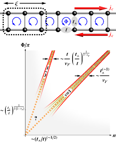
Figure 1: Top: Two-leg ladder model with magnetic flux per plaquette $\Phi$ leading to chiral currents $j_{c}$ flowing around the ladder. $\xi$ denotes interaction range. Bottom: Schematic fermionic chiral current contours of Eq. (2) marked by thin lines in the $n$-$\Phi$ plane, within an integer and a fractional QH phase. The phase transition lines out of the QH states are marked by solid thick lines, and the thick dotted lines correspond to fillings ${n=\nu\Phi/\pi}$. The validity regime is discussed in the text.

The aim of this paper is (i) to analytically establish realizations of FQH phases in concrete 1D lattice models and (ii) propose a physical quantity that unambiguously signals these phases’ fractional quantum Hall nature. By FQH in 1D, we refer to the coupled wire construction introduced by Kane et al. kan . While the 2D limit of this construction corresponds to the robust quantum Hall liquid, we herein study the thin-stripe regime, in which the system is sensitive to small perturbations, and hence finding detectable signatures is more demanding.

In Sec. II, we introduce the instructive noninteracting integer model; in Sec. III, we elaborate on the realizations of fractional quantum Hall states in 1D two-leg ladders of either interacting bosons or interacting fermions. These FQH instabilities occur when the 1D density $n$ is related to the flux per plaquette $\Phi$ as

$$n=\nu\frac{\Phi}{\pi},$$ (1)

with ${\nu=1/m}$, and where $m$ is either odd for fermions or even for bosons; see dotted lines in Fig. 1. The FQH phases support finite deviations from this density, as schematically shown in Fig. 1, which increase with the inter-chain coupling $t_{\perp}$ and represent the finite compressibility of the system analogous to the 2D edge states. Upon increasing the range of interactions, we find that arbitrary Laughlin ${\nu=1/m}$ states can be stabilized even at small inter-chain coupling. The required range of interactions increases Barbarino et al. (2015) for low filling factors; the ${\nu=1/3}$ state already requires interactions between nearest neighbour rungs, while the ${\nu=1/2}$ bosonic state is stabilized for sufficiently strong but only on-rung interactions Petrescu and Le Hur (2015). Interestingly, in the synthetic dimension realizations of quantum ladders, the interactions become non-local in the synthetic dimension Mancini et al. (2015); Stuhl et al. (2015); Yan et al. (2015) (along the rungs), allowing one to reach this bosonic FQH state.

In Sec. IV, we address the question: What are manifestations of the FQHE in 1D ladders? In Refs. Oreg et al., 2014; Meng et al., 2014; Cornfeld et al., 2015 transport was considered through leads connected to the 1D fractional helical state. In contrast, we herein wish to discuss thermodynamic bulk observables which may be detected in cold-atom experiments and simple simulations, where transport can not be directly measured. Such an observable is the chiral current $j_{c}$ that flows in the ground state due to the magnetic flux; see Fig. 1. The possibility that chiral currents screen the orbital magnetic field in a kind of a Meissner phase, was pointed out Orignac and Giamarchi (2001); Petrescu and Le Hur (2013); Piraud et al. (2015) and recently observed experimentally Atala et al. (2014); Mue ; here we focus on the FQH phase.

We show that within the FQH phase the current depends on density $n$ and flux $\Phi$ as

$$j_{c}\propto\left(n-\frac{\nu}{\pi}\Phi\right),$$ (2)

up corrections that vanish for small inter-chain coupling $t_{\perp}$ and are discussed in detail in Sec. IV. Therefore, for small $t_{\perp}$, the behaviour described by Eq. (2) can be detected in the current map of the $n$-$\Phi$ plane as shown in Fig. 1; contours of constant current are asymptotically parallel to the constant filling factor line, Eq. (1), which is depicted by the dotted line in Fig. 1.

These current contour are determined by the fractional filling $\nu$ and hence allows one to measure it. As we show, this result implies the emergence of fractional “edge” states on the two-leg ladder and thus forms a stringent test for the stabilization of FQH states in ladders. The constraints on the validity regime of this result are discussed in Secs. III.1 and IV.3. Under these constraints the phase diagram in Fig. 1 is exhaustive and no additional phases occur.

We conclude in Sec. V providing perspectives on the experimental relevance in ultracold-atomic systems.

II Noninteracting model

We consider a spinless two-leg ladder of either fermions or bosons as shown in Fig. 1. Our main attention in this paper is devoted to the combined effect of interactions and magnetic flux $\Phi$. It is instructive, however, to first display the simple physics of the noninteracting fermionic model, and investigate the properties of the chiral currents in this simpler case, as done in this section.

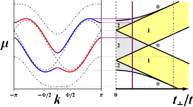
Figure 2: Left: dispersion relation $\epsilon_{k}^{\pm}$ for representative values of $t_{\perp}/t$. Right: phase diagram for noninteracting fermions; ${c=0,1,2}$ labels the number of pairs of Fermi points (central charge).

The noninteracting model Hamiltonian is $H=H_{0}+H_{\perp}$, where

$$H_{0}=-t\sum_{j,y}\left(c^{\dagger}_{j,y}c^{\phantom{\dagger}}_{j+1,y}+\mathrm{h.c.}\right)$$ (3)

describes hopping within each chain ${y=1,2}$, and the inter-chain hopping is

$$H_{\perp}=-t_{\perp}\sum_{j}\left(c^{\dagger}_{j,1}c^{\phantom{\dagger}}_{j,2}e^{i\Phi j}+\mathrm{h.c.}\right).$$ (4)

Here $\Phi$ is the magnetic flux per plaquette. It is convenient to make the gauge transformation ${c^{\prime}_{j1}=c_{j1}e^{-i\frac{1}{2}\Phi j}}$, ${c^{\prime}_{j2}=c_{j2}e^{i\frac{1}{2}\Phi j}}$, which moves the phase factor $e^{i\Phi j}$ from inter- to intra-chain hopping, yielding the Bloch Hamiltonian

$$H_{k}=\left(\begin{array}[]{cc}-2t\cos(k-\frac{\Phi}{2})&t_{\perp}\\ t_{\perp}&-2t\cos(k+\frac{\Phi}{2})\\ \end{array}\right)$$ (5)

(the lattice constant is set to unity). Its eigenvalues $\epsilon_{k}^{\pm}$ are plotted in Fig. 2 for various values of $t_{\perp}/t$. At ${t_{\perp}=0}$ we have two cosine dispersions shifted horizontally by ${\pm\frac{\Phi}{2}}$ (dashed lines). Any small inter-chain coupling $t_{\perp}$ opens a gap at the crossing points (full lines). As seen in the right panel of Fig. 2, upon scanning the chemical potential one finds two partially gapped “chiral” regions with only one pair (${c=1}$) [rather than two pairs (${c=2}$)] of Fermi points, where $c$ denotes the central charge. In these chiral phases, the left- and right-moving modes reside on distinct chains; see color code in Fig. 2. Upon further increasing $t_{\perp}$, the chiral nature of the 1D modes is gradually reduced, and one eventually obtains (dot-dashed) dispersion curves which are nonoverlapping bands dominated by the inter-chain hopping.

We shall focus on the regime of ${t_{\perp}\ll t}$ near the instability leading to the opening of the lower partially gapped ${c=1}$ region in the the phase diagram. The particle density is defined as ${n=\sum_{y=1,2}\langle c^{\dagger}_{j,y}c^{\phantom{\dagger}}_{j,y}\rangle}$, and the gap opens at the Fermi level when ${n=\frac{\Phi}{\pi}}$. Borrowing the 2D definition of filling factor, namely the ratio of particle density per site, ${\langle c^{\dagger}_{j,y}c^{\phantom{\dagger}}_{j,y}\rangle=\frac{n}{2}}$, to the density of flux quanta per plaquette,

$$\nu=\frac{\pi n}{\Phi},$$ (6)

we see that the gap opening at small $t_{\perp}$ occurs at unit filling factor ${\nu=1}$. This gap opening is just the two wire version of the wire-construction of the quantum Hall effect kan . One pair of modes is gapped out, and one pair remains gapless in analogy with the chiral edge states in the integer quantum Hall effect.

The two-leg ladder is equivalent to a Rashba wire upon reinterpretation of (i) the two legs of the ladder as a spin degree of freedom, (ii) the inter-chain hopping $t_{\perp}$ as a spin-flipping Zeeman field, and (iii) the magnetic flux $\Phi$ as a Rashba spin orbit coupling causing a momentum shift ${\pm k_{SO}}$ of the two dispersions,

$$\begin{array}[]{ccc}y=1,2&\leftrightarrow&\sigma=\uparrow,\downarrow,\\ t_{\perp}&\leftrightarrow&B_{\mathrm{Zeeman}},\\ \Phi&\leftrightarrow&2k_{\mathrm{SO}}.\end{array}$$ (7)

After this relabeling of indices and parameters, the partially gapped chiral state with ${c=1}$ corresponds to a helical state with the two spins propagating to opposite directions Oreg et al. (2010); Lutchyn et al. (2010). In this context, $j_{c}$ is simply a persistent spin current Yi . We next discuss the persistent current $j_{c}$ generated by the magnetic flux in the two-leg ladder.

II.1 Chiral current in the $n$-$\Phi$ plane

The magnetic flux induces a persistent current in the ground state (GS), see Fig. 1,

$$j_{c}=-\left\langle\frac{\partial H}{\partial\Phi_{\mathrm{tot}}}\right\rangle_{\mathrm{GS}}=-\frac{1}{L}\frac{\partial E_{\mathrm{GS}}}{\partial\Phi},$$ (8)

where ${\Phi_{\mathrm{tot}}=L\Phi}$ is the total flux in a two-leg ladder of length $L$. Here, we expressed the current as the derivative of the ground state energy ${E_{\mathrm{GS}}=\langle H\rangle_{\mathrm{GS}}}$ with respect to $\Phi$. We shall see that the current can be used to probe 1D quantum Hall physics.

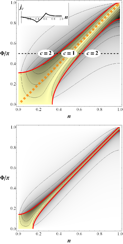
Figure 3: Contours of the chiral current $j_{c}$ marked by thin lines in the $\Phi$-$n$ plane for ${t_{\perp}=0.5t}$ (top) and ${t_{\perp}=0.1t}$ (bottom). The phase transition lines are marked by solid thick lines, and the thick dotted line corresponds to ${n=\Phi/\pi}$. The inset (top) depicts the chiral current along the horizontal dashed line.

One may explore the current dependence on density $n$ and flux $\Phi$. In a noninteracting model the ground state energy is the sum over individual occupied states. In the ${c=1}$ regime only one band contributes,

$$j_{c}(n,\Phi)=-\int_{-\pi n}^{\pi n}\frac{dk}{2\pi}\frac{\partial\epsilon_{k}^{-}}{\partial\Phi}.$$ (9)

The contours of ${j_{c}(n,\Phi)}$ are plotted in Fig. 3 for two values of ${t_{\perp}/t}$ both in and out of the chiral ${c=1}$ phase. The phase transitions are marked as thick red lines, and the current has cusp singularities at these transitions, as shown in the inset. We see that within the ${c=1}$ chiral phase and for not too small a density, the current contours are approximately parallel to the line defined in Eq. (6). This behaviour becomes more pronounced as ${t_{\perp}/t}$ becomes smaller; see lower panel of Fig. 3.

For a quantitative description of this assertion we decompose the symmetric integral Eq. (9) into contributions from the Fermi sea and from near the Fermi surface (${n\simeq\frac{1}{\pi}\Phi}$), as ${j_{c}=j_{c}^{\mathrm{sea}}+j_{c}^{\mathrm{surf}}}$, where

$$j_{c}^{\mathrm{sea}}=-\int_{0}^{\Phi}\frac{dk}{\pi}\frac{\partial\epsilon_{k}^{-}}{\partial\Phi},~{}~{}~{}j_{c}^{\mathrm{surf}}=-\int_{\Phi}^{\pi n}\frac{dk}{\pi}\frac{\partial\epsilon_{k}^{-}}{\partial\Phi}.$$ (10)

Relegating details to Appendix A, using this decomposition we find that the total current satisfies

$$(\partial_{n}+\pi\partial_{\Phi})j_{c}=A^{\mathrm{surf}}\cdot(n-\tfrac{\Phi}{\pi})+A^{\mathrm{sea}}\cdot\tfrac{t_{\perp}^{2}}{t^{2}}\ln\tfrac{t}{t_{\perp}}+\mathcal{O}(\tfrac{t_{\perp}^{2}}{t^{2}}).$$ (11)

The two terms in the right hand side arise from the Fermi surface and the Fermi sea, their coefficients $A^{\mathrm{surf}}$ and $A^{\mathrm{sea}}$ are derived in Appendix A. The Fermi surface contribution originates from the band curvature and is given by ${A^{\mathrm{surf}}=\tfrac{1}{4\pi}\partial_{n}^{2}\mu}$.

As herein explained, two terms on the right hand side of Eq. (11) form a small correction. If one tunes the density to the exact filling factor ${\nu=1}$, the first correction term vanishes. Deviations of the density ${\delta n}$ within the ${c=1}$ phase are of the order of the energy gap ${E_{\mathrm{gap}}=\epsilon_{k=0}^{+}-\epsilon_{k=0}^{-}=2t_{\perp}}$ times the density of states $\frac{1}{\pi v_{F}}$, where $v_{F}$ is the Fermi velocity. The first correction term thus approaches values of order ${\mathcal{O}(t_{\perp}/t)}$ near the boundaries of the ${c=1}$ region. As a consequence, this leading correction, as well as the second term and other subleading corrections, are altogether negligible for small inter-chain coupling, ${t_{\perp}\ll t}$, resulting in ${(\partial_{n}+\pi\partial_{\Phi})j_{c}\simeq 0}$. It implies that indeed, contours of the current are nearly parallel to the dashed line ${n=\Phi/\pi}$ as seen in Fig. 3 for gradually decreasing $t_{\perp}$.

This behaviour is valid for density ${\sqrt{t_{\perp}/t}\ll n\ll 1}$. For too small a density, one reaches the situation where the Fermi energy ${\thicksim tn^{2}}$ becomes smaller than the energy gap ${\thicksim t_{\perp}}$, giving the lower bound. For too high a density of order unity, the partial gaps of electrons and holes (see Fig. 2) approach each other and cause undesired lattice effects. Thus, for ${t_{\perp}/t\ll 1}$ we have a large region in the parameter space where the contours are asymptotically parallel to ${n=\Phi/\pi}$. This is a general feature which holds true for the interacting fractional case, as we find in Sec. IV.

III Fractional states in lattice models with long range interactions

We now consider either interacting fermions or bosons on the two-leg ladder, and add interactions to the lattice model, ${H=H_{0}+H_{\perp}+H_{\mathrm{int}}}$, with

$$H_{\mathrm{int}}=\sum_{r\geq 0}V(r)\sum_{j}n_{j}n_{j+r}.$$ (12)

Here, ${c^{\phantom{\dagger}}_{j,y}c^{\dagger}_{j^{\prime},y^{\prime}}-(+)c^{\dagger}_{j^{\prime},y^{\prime}}c^{\phantom{\dagger}}_{j,y}=\delta_{y,y^{\prime}}\delta_{j,j^{\prime}}}$ for bosons (fermions) and, ${n_{j}=\sum_{y=1,2}c^{\dagger}_{j,y}c^{\phantom{\dagger}}_{j,y}}$. In this model, the interaction potential is independent of the rungs’ indices $y$ and $y^{\prime}$, and depends solely on the linear distance $r$ via ${V(r)}$, specified below. Similar to the Hubbard model, the dependence of the interaction only on the total density ${\sum_{y}c^{\dagger}_{j,y}c^{\phantom{\dagger}}_{j,y}}$ makes the model ${H_{0}+H_{\mathrm{int}}}$ to be ${\mathrm{SU}(2)}$ invariant with respect to rotations of the spinor ${(c_{j,1},c_{j,2})}$.

To treat these interactions, we utilize the Luttinger liquid theory. For a generic interaction $H_{\mathrm{int}}$ and at ${t_{\perp}=0}$, the long wavelength behaviour of the quantum ladder can be described by a two component Luttinger liquid (LL) Gia . The free part of the Hamiltonian is expressible in terms of the density operators of the two chains. It is convenient to introduce bosonic fields $\phi_{\mu}$, so that the long wavelength fluctuations of the total charge $(\rho)$ and the relative density ($\sigma$), denoted “charge” and “spin”, respectively, are represented by

$$c^{\dagger}_{j,1}c^{\phantom{\dagger}}_{j,1}+c^{\dagger}_{j,2}c^{\phantom{\dagger}}_{j,2} \thicksim n-\frac{\sqrt{2}}{\pi}\nabla\phi_{\rho}(x),\hbox{ and}$$

$$c^{\dagger}_{j,1}c^{\phantom{\dagger}}_{j,1}-c^{\dagger}_{j,2}c^{\phantom{\dagger}}_{j,2} \thicksim-\frac{\sqrt{2}}{\pi}\nabla\phi_{\sigma}(x).$$ (13)

The free Hamiltonian can be written as

$$\mathcal{H}_{\mathrm{LL}}=\sum_{\mu=\rho,\sigma}\frac{1}{2\pi}\int dx\left[v_{\mu}K_{\mu}(\pi\Pi_{\mu})^{2}+\frac{v_{\mu}}{K_{\mu}}(\nabla\phi_{\mu})^{2}\right],$$ (14)

where the $\Pi_{\mu}$ fields are canonically conjugate to the densities, ${[\phi_{\mu}(x),\Pi_{\nu}(x^{\prime})]=i\delta_{\mu\nu}\delta(x-x^{\prime})}$. The velocities $v_{\rho,\sigma}$ and LL parameters $K_{\rho,\sigma}$ depend on the strength of interactions and on the density; in the noninteracting fermionic case ${K_{\rho}=K_{\sigma}=1}$ and ${v_{\rho}=v_{\sigma}=v_{F}}$. Note, that for generic interactions, one still has ${K_{\sigma}=1}$ if the model is SU(2) symmetric Gia , as holds true in our model at ${t_{\perp}=0}$.

The remaining of the section is divided into two parts. We first list the possible perturbations to the Luttinger liquid model Orignac and Giamarchi (2001); Oreg et al. (2014); Petrescu and Le Hur (2013), which include the FQH instability on which we focus. This enables one to obtain conditions for the Luttinger liquid parameter $K_{\rho}$ and density $n$, under which operators identified as opening FQH gaps are most relevant in the renormalization group (RG) sense. We then discuss a specific form of the interaction ${V(r)}$, corresponding to a finite range with hard core interactions, for which $K_{\rho}$ can be computed exactly for ${t_{\perp}=0}$, assuring that the FQH instability dominates for finite small inter-chain coupling $t_{\perp}$.

III.1 Luttinger liquid instabilities

There are various operators correcting the LL Hamiltonian. We may group them as ${\mathcal{H}=\mathcal{H}_{\mathrm{LL}}+\delta\mathcal{H}+\delta\mathcal{H}_{\perp}}$, where ${\delta\mathcal{H}_{\perp}}$ includes terms generated by $t_{\perp}$, while ${\delta\mathcal{H}}$ includes terms which exist at ${t_{\perp}=0}$. We systematically list these various operators in Appendix B.

The interesting FQH physics would not occur without the inter-chain coupling

$$c^{\dagger}_{j1}c^{\phantom{\dagger}}_{j2}e^{i\Phi j}+\mathrm{h.c.}.$$ (15)

We may express the particle creation and annihilation operators in the bosonized language,

$$\begin{gathered}c^{\dagger}_{j,y}\to\Psi^{\dagger}_{y}(x)\sim\sum_{p}\psi^{\dagger}_{y,p}(x),\\ \psi_{y,p}^{\dagger}(x)=e^{i2p(\pi\frac{n}{2}x-\phi_{y}(x))}e^{-i\theta_{y}(x)}\\ \phi_{\rho,\sigma}=\tfrac{\phi_{1}\pm\phi_{2}}{\sqrt{2}},~{}~{}\theta_{\rho,\sigma}=\tfrac{\theta_{1}\pm\theta_{2}}{\sqrt{2}},~{}~{}~{}\pi\Pi_{\mu}=\nabla\theta_{\mu}(x),\end{gathered}$$ (16)

where the sum over $p$ runs over integers for bosons or half integers for fermions Gia . The operators generated by this expansion are of the form

$$\mathcal{O}_{p}\thicksim\psi^{\dagger}_{1,-p}\psi^{\phantom{\dagger}}_{2,p}e^{i\Phi x}+\mathrm{h.c.}.$$ (17)

Such operators may be incorporated into the bosonised LL Hamiltonian using

$$\mathcal{O}_{p}\thicksim g_{p}\int dx\cos(\sqrt{2}\theta_{\sigma}-2p\sqrt{2}\phi_{\rho}-(\Phi-2p\pi n)x),$$ (18)

with a coupling constant $g_{p}$ generated by interactions and by the inter-chain coupling $t_{\perp}$. These operators are oscillating unless

$$2p\pi n=\Phi.$$ (19)

When relevant, such operators may open an energy gap even for a finite deviation from this exact flux up to a commensurate-incommensurate transition Orignac and Giamarchi (2001); Petrescu and Le Hur (2013). The above condition is met when the filling factor Eq. (6) is given by

$$\nu=\frac{1}{2p},$$ (20)

which is the inverse of an even(odd) integer for bosons(fermions). The states generated by this operator correspond to the Laughlin FQH phases as constructed by coupled wires kan . The scaling dimension of $\mathcal{O}_{p}$ is given by

$$x_{p}=\frac{1}{2}\left(\frac{1}{K_{\sigma}}+(2p)^{2}K_{\rho}\right).$$ (21)

In the ${\mathrm{SU}(2)}$ symmetric case of ${K_{\sigma}=1}$, its relevancy ${x_{p}<2}$ is ensured by a small value of the charge LL parameter

$$K_{\rho}<\frac{3}{(2p)^{2}}=3\nu^{2}.$$ (22)

In this symmetric case, usual RG analysis Gia shows that the energy gap scales as

$$E_{\mathrm{gap}}\thicksim t(t_{\perp}/t)^{\frac{1}{2-x_{p}}}.$$ (23)

In the noninteracting case for example, the scaling dimension equals ${x_{p}=1}$ which is consistent with the energy gap ${E_{\mathrm{gap}}=2t_{\perp}}$.

Additional phases generated by $t_{\perp}$, described in Ref. Petrescu and Le Hur, 2015, are included for completeness in Appendix B, such as the Meissner phase and the vortex lattice Orignac and Giamarchi (2001). In order to stabilize a given FQH state, one needs to (i) have a small value of $K_{\rho}$ satisfying Eq. (22), and (ii) make sure that other instabilities are less relevant. Below we consider a specific interaction ${V(r)}$ with a finite range $\xi$, and determine the range required to satisfy these conditions and observe a FQH state at any desired fractional filling $\nu$.

III.2 Solvable Lattice Model

We now specialize to an interaction potential that vanishes beyond the interaction range $\xi$, see Fig. 1,

$$V(r)=\begin{cases}Uv(r)&\mbox{for }r\leq\xi,\\ 0&\mbox{for }r>\xi.\end{cases}$$ (24)

Here, ${v(r)}$ is a positive decreasing function whose specific form is not important, with ${v(0)=1}$ and ${v(r)=\mathcal{O}(1)}$ for ${r\leq\xi}$. The case $\xi=0$ corresponds to on-rung interactions, namely ${V(r=0)}$ comprises both on-site interactions (meaningful for bosons) and interactions between particles on different sites of the same rung (as in the Hubbard model).

We focus on the regime ${U\gg t}$, for general interaction range $\xi$. The analysis starts by assuming infinite $U$, for which ${H_{0}+H_{\mathrm{int}}}$ is exactly solvable, and then relaxes this assumption to finite but large $U$. In this hard-core limit, the interaction becomes a constraint: states containing two particles horizontally separated by $\xi$ sites or less acquire a very high energy ${\mathcal{O}(U)}$. One can construct a low-energy subspace where the shortest linear inter-particle distance exceeds $\xi$. The allowed states for $N$ bosonic or fermionic particles on the ladder of length $L$ and open boundary conditions are then in one to one correspondence Sela and Pereira (2011); Sela et al. (2011) with the states of a constrained model. This model consists of $N$ fictitious particles on a ladder of reduced length ${L^{\prime}=L-(N-1)\xi}$ subject to an additional constraint of not having two fictitious particles on the same rung. Each particle in the reduced lattice corresponds to one particle and $\xi$ empty rungs to its right on the original lattice.

For ${t_{\perp}=0}$, the leg index ${y=1,2}$ of each particle is conserved i.e. the sequence of $y$ values for $N$ particles from left to right ${\{y_{1},y_{2},...,y_{N}\}}$ is conserved (considering open boundary conditions for simplicity). For a fixed value of this list, the $\xi-$constrained motion of the $N$ particles, with states labeled by ${\{j_{1},j_{2},...,j_{N}\}}$ on the ladder, becomes equivalent to free fermions on a single chain of length $L^{\prime}$; the Pauli principle fully accounts for the interaction constraint. Following the methods described in Ref. Sela et al., 2011 and detailed in Appendix C, we find that the Luttinger liquid parameter describing the model ${H_{0}+H_{\mathrm{int}}}$ depends on the density per rung $n$ and interaction range $\xi$ as

$$K_{\rho}\xrightarrow[U\to\infty]{}\frac{1}{2}(1-n\xi)^{2}.$$ (25)

For ${\xi=0}$ this result coincides with the exact solution of the Hubbard model i.e. ${K_{\rho}=\frac{1}{2}}$ for infinite repulsion. This result enables us to choose values for $\xi$ and $n$ that yield a sufficiently small $K_{\rho}$ that satisfies Eq. (22). Thus we can use the exact solvability of ${H_{0}+H_{\mathrm{int}}}$, and proceed using usual RG methods to treat $t_{\perp}$ as a perturbation, and deduce under which conditions is the FQH cosine perturbation relevant and flows to strong coupling.

The Luttinger parameter ${K_{\rho}=K_{\rho}[U/t]}$ is a continuous decreasing function of ${U/t}$, hence having a large enough but finite value of ${U/t}$ leads only to negligible (positive) corrections to the lower bound of $K_{\rho}$ in Eq. (25). At the same time, as is known for the Hubbard model, in the strict ${U=\infty}$ limit one has a vanishing spin velocity ${v_{\sigma}\to 0}$, making the Luttinger liquid description pathological. This is not the case, however, for finite $U$ on which we focus, where the spin velocity remains finite.

In the infinite $U$ limit and for an interaction range $\xi$, the maximal possible density is ${n<\frac{1}{1+\xi}}$. On the other hand, Eq. (25) and the relevancy condition Eq. (22) impose a minimal possible density as well,

$$\frac{1-\sqrt{6}\nu}{\xi}<n<\frac{1}{1+\xi}.$$ (26)

Comparing the minimal and maximal densities, one finds that the required interaction range for a relevant FQH perturbation at filling factor $\nu$ is

$$\xi\geq\left\lceil\frac{1}{\sqrt{6}\nu}-1\right\rceil.$$ (27)

For bosons at ${\nu=1/2}$, this relevancy condition is satisfied for on-rung interactions ${\xi=0}$ Petrescu and Le Hur (2013). However for fermions at ${\nu=1/3}$, or bosons at ${\nu=1/4}$, one needs at least nearest neighbour interactions, ${\xi=1}$. This is summarized in Table 1.

Table 1: Conditions for the realization of the 1D FQH states at filling factor $\nu$ in a two-leg ladder with hard-core interaction of range $\xi$ given in Eq. (26) and Eq. (27) .

	$\nu=\frac{1}{2}$	$\nu=\frac{1}{3}$	$\nu=\frac{1}{4}$	$\nu=\frac{1}{5}$
$\xi=0$	$0<n$	-	-	-	$n<1$
$\xi=1$	$0<n$	$0.18<n$	$0.38<n$	-	$n<0.5$
$\xi=2$	$0<n$	$0.09<n$	$0.19<n$	$0.25<n$	$n<0.33$
$\xi=3$	$0<n$	$0.06<n$	$0.12<n$	$0.17<n$	$n<0.25$

Note, that in the hard core limit with interaction range $\xi$, the kinetic motion freezes at the maximal allowed density of ${n=\frac{1}{1+\xi}}$. This corresponds to a Mott insulating state. However, this charge-density wave (CDW) instability is not relevant and hence prevented for ${n<\frac{1}{1+\xi}}$. Going through the list of operators detailed in Appendix B we find that there are no other nonoscillating relevant operators that compete with the relevant FQH operator Eq. (18).

III.2.1 Spin lattice implementation of hard core bosons

We discuss a simplification and a specific implementation of the bosonic ${\nu=1/2}$ state for on-rung interactions $\xi=0$. In order to substantially reduce the size of the Hilbert space keeping the essential physics intact, as we are interested in the limit of large $U$, we can switch from bosons, to a spin-$1/2$ lattice Piraud et al. (2015), using the replacement

$$c^{\dagger}_{j,y}\rightarrow S^{+}_{j,y},~{}~{}~{}~{}c_{j,y}\rightarrow S_{j,y}^{-},~{}~{}~{}n_{j}\rightarrow 1+\sum_{y=1,2}S^{z}_{j,y}.$$ (28)

The two-leg ladder model becomes

$$H =-t\sum_{j,y=1,2}\left(S^{+}_{j,y}S^{-}_{j+1,y}+\mathrm{h.c.}\right)$$

$$-t_{\perp}\sum_{j}\left(S^{+}_{j,1}S^{-}_{j,2}e^{i\Phi j}+\mathrm{h.c.}\right)$$

$$+2U\sum_{j}S^{z}_{j,1}S^{z}_{j,2}.$$ (29)

Recently, integer Chern insulating phases have been directly discussed in similar XY spin chains Graß et al. (2015) with a synthetic magnetic flux.

As a self-consistent example, one may consider a ladder of length ${L\thicksim 100}$ in the vicinity of ${\Phi=0.8\pi}$ and ${n=0.4}$ (or equivalently ${\langle S^{z}\rangle=-0.3}$). There are 2 particles (up spins) every 5 rungs, and hence, given the short range repulsion, the system is far from any CDW instability. For this setup, ${x_{p}=3/2}$ and the gap scales as ${E_{gap}\thicksim t(t_{\perp}/t)^{2}}$. The length scale over which the gap is formed scales as

$$\ell^{*}\thicksim(t/t_{\perp})^{2}.$$ (30)

The length of the ladder, $L$, should be larger than this crossover scale for the RG flow to fully develop the cosine perturbation from weak to strong coupling. This limits the inter-chain coupling ${t_{\perp}/}t$ to be not smaller than of order ${\sim 10^{-1}}$.

To conclude this section, we have shown that FQH states occur as ground states in two-leg ladders with interactions of sufficiently long range. However, what are signatures of the fractional filling in these ground states? Below, we shall focus on this question.

IV Chiral current

So far we have discussed explicit lattice realizations of FQH states in 1D ladders. However, when such models are realized, e.g. in an experiment or a numerical simulation, it is not obvious what are their signatures. Here, we explore the chiral current flowing around the ladder, and find signatures in the $n$-$\Phi$ plane that are characteristic of the fractional filling factor $\nu$, generalizing the behaviour found for the noninteracting case in Sec. II.1.

The below calculation of the current and its derivatives with respect to $\Phi$ and $n$ is done using bosonization. It is known that all filled states contribute to the chiral current, which is a persistent current; the chiral current in the ladder is thus generally not an infra-red phenomenon and cannot be fully accounted for by an effective low-energy theory Narozhny et al. (2005); Carr et al. (2006). Nevertheless, certain aspects of the persistent current, such as its derivative with respect to particle number or flux, can be computed from the low-energy theory Simon and Affleck (2001). Indeed, in Sec. II.1, we have identified two contributions to the current in the noninteracting case, one of which is a Fermi surface effect and the other is a Fermi sea effect. When generalizing to the interacting fractional case, the former can be safely extracted from the low-energy theory of bosonization.

We take the following three steps which eventually provide a complete picture of the current in the $n$-$\Phi$ plane: (i) In Sec. IV.1, we analyse the effects of the cosine perturbation Eq. (18), which being a relevant operator, flows to strong coupling ${g_{p}\to\infty}$. It yields straight current contours parallel to the line ${n=\nu\Phi/\pi}$. (ii) Then, in Sec. IV.2, we include band curvature irrelevant cubic terms, such as ${(\nabla\phi_{\rho})^{3}}$, in the bosonized Hamiltonian; see Eq. (42) below. These terms contribute to corrections analogous to the term ${A^{\mathrm{surf}}\cdot(n-\frac{\Phi}{\pi})}$ in Eq. (11), and signal deviations of the density from the exact fractional filling. (iii) Finally, in Sec. IV.3, we add additional quadratic operators in the LL theory which were not allowed at ${t_{\perp}=0}$, such as

$$\nabla\phi_{\rho}\nabla\theta_{\sigma},~{}~{}~{}{\mathrm{and}}~{}~{}~{}\nabla\phi_{\sigma}\nabla\theta_{\rho}.$$ (31)

These corrections give additional distortions of the current contours, which may be nevertheless neglected for small ${(t_{\perp}/t)^{2}}$.

The result of these calculations is summarized in the schematic Fig. 1.

IV.1 Chiral current in FQH states

We treat $v_{\rho,\sigma}$ and $K_{\rho,\sigma}$ in Eq. (14) as the effective parameters resulting from the RG flow, and treat the strong coupling limit of Eq. (18). We wish to find a relation between the three susceptibilities

$$\chi_{ab}=\frac{1}{L}\frac{\partial^{2}E_{\mathrm{GS}}}{\partial a\partial b},~{}~{}~{}a,b=n,\Phi.$$ (32)

Here $\chi_{nn}$ is the charge susceptibility, $\chi_{\Phi\Phi}$ is the diamagnetic susceptibility, and the mixed susceptibility ${\chi_{n\Phi}=\chi_{\Phi n}}$ describes the change of the persistent current ${j_{c}=-\frac{1}{L}\partial_{\Phi}E_{\mathrm{GS}}}$ with respect to particle addition.

We may opt to treat the fields $\phi_{\rho},\theta_{\sigma}$ as generalized coordinates ($q$) and their canonical conjugates $\nabla\theta_{\rho},\nabla\phi_{\sigma}$ as momenta ($p$). This is a useful choice as the Hamiltonian naturally decomposes to ${\mathcal{H}=\mathcal{H}_{p}+\mathcal{H}_{q}}$ as

$$\mathcal{H}_{p}=\frac{1}{2\pi} \int dx\left[v_{\rho}K_{\rho}(\nabla\theta_{\rho})^{2}+\frac{v_{\sigma}}{K_{\sigma}}(\nabla\phi_{\sigma})^{2}\right],$$ (33)

$$\mathcal{H}_{q}=\frac{1}{2\pi} \int dx\left[\frac{v_{\rho}}{K_{\rho}}(\nabla\phi_{\rho})^{2}+v_{\sigma}K_{\sigma}(\nabla\theta_{\sigma})^{2}\right]$$

$$+g_{p} \int dx\cos\left(\sqrt{2}\theta_{\sigma}-\sqrt{2}\nu^{-1}\phi_{\rho}+\delta\Phi x\right),$$ (34)

where ${\delta\Phi=\Phi-\tfrac{\pi n}{\nu}}$. The argument of the cosine is pinned in the strong coupling limit and we thus integrate out the $\theta_{\sigma}$ field so the Hamiltonian $\mathcal{H}_{q}$ takes the form

$$\mathcal{H}_{q}=\frac{1}{2\pi}\int dx\left[v_{\sigma}K_{\sigma}(\tfrac{1}{\nu}\nabla\phi_{\rho}+\tfrac{1}{\sqrt{2}}\delta\Phi)^{2}+\frac{v_{\rho}}{K_{\rho}}(\nabla\phi_{\rho})^{2}\right].$$ (35)

By recalling Eq. (III) one sees that a variation of the density is equivalent to setting ${\nabla\phi_{\rho}=-\frac{\pi}{\sqrt{2}}\delta n}$, and hence

$$\tfrac{1}{L}E_{\mathrm{GS}}\simeq\frac{\pi}{4}\left[v_{\sigma}K_{\sigma}(\tfrac{1}{\nu}\delta n-\tfrac{1}{\pi}\delta\Phi)^{2}+\frac{v_{\rho}}{K_{\rho}}{\delta n}^{2}\right].$$ (36)

Notice that both “momenta” fields $\theta_{\rho},\phi_{\sigma}$ appear quadratically in $\mathcal{H}_{p}$ and it may be rigorously integrated out by choosing the gauge of ${\partial_{t}\Phi=0}$ in the Lagrangian formalism. This allows us to directly read off the susceptibilities

$$\chi_{n\Phi}=-\frac{1}{2\nu}v_{\sigma}K_{\sigma},~{}~{}~{}\chi_{\Phi\Phi}=\frac{1}{2\pi}v_{\sigma}K_{\sigma},$$

$$\chi_{nn}=\frac{\pi}{2}\left(\frac{v_{\rho}}{K_{\rho}}+\frac{1}{\nu^{2}}v_{\sigma}K_{\sigma}\right).$$ (37)

The relation ${\partial_{n}\partial_{\Phi}E_{\mathrm{GS}}=-\frac{\pi}{\nu}\partial_{\Phi}\partial_{\Phi}E_{\mathrm{GS}}}$ allows one to extract the fractional filling factor $\nu$ from a ratio of two thermodynamic susceptibilities. Equivalently, from the definition of the chiral current Eq. (8) we obtain

$$\left(\partial_{n}+\frac{\pi}{\nu}\partial_{\Phi}\right)j_{c}=0.$$ (38)

Notice that this relation does not depend on any of the LL parameters. Below we see that corrections to this relation are only of order ${\mathcal{O}(\delta n,\delta\Phi)}$ and are thus small in ${t_{\perp}/t}$. Moreover, the current can be obtained by differentiation of Eq. (36),

$$j_{c}=\frac{1}{2\nu}K_{\sigma}v_{\sigma}\left(n-\frac{\nu}{\pi}\Phi\right).$$ (39)

These results suggest that in the $n$-$\Phi$ plane the current is constant parallel to the line of fractional filling, ${n=\nu\Phi/\pi}$, within the partially gapped phase; see dotted lines in Fig. 1.

It is desirable to arrive at a physical interpretation of these results (for this discussion, we retain the electron charge $e$ and Plank constant $\hbar$).

Consider the physics on the edge of an incompressible FQH droplet at filling factor ${\nu=1/m}$. The dynamical degree of freedom is the density of the chiral edge, $n_{c}$, which is a deformation of the edge of the incompressible liquid wen ; the chiral current is given by ${j_{c}=evn_{c}}$, where $v$ is the velocity of the edge. Electrodynamics on the edge is quite unusual, as the electron charge is intrinsically entangled with the electromagnetic potential on the edge Eza

$$n_{c}\to n_{c}-\frac{e}{2\pi m\hbar}A_{\parallel}.$$ (40)

It coincides with the minimal substitution argument for the vector potential $A_{\parallel}$ along the edge. This implies Eza the celebrated Laughlin argument of an adiabatic insertion of a flux quantum ${\delta A_{\parallel}=\frac{2\pi\hbar}{eL_{\mathrm{edge}}}}$ leading to the total change in the charge of the edge by a fractional amount ${e/m}$ (and creating a quasihole in the flux insertion point). As a consequence, Eq. (40) demonstrates that the current

$$j_{c}=ev\left(n_{c}-\frac{e}{2\pi m\hbar}A_{\parallel}\right),$$ (41)

remains invariant for a simultaneous change of the particle number and of the magnetic flux while keeping their ratio pinned to the filling factor. The two-leg ladder thus can be thought of as an ultra thin FQH droplet, with one chiral edge on the ${y=1}$ sites and the opposite chiral edge on the ${y=2}$ sites. We conclude that the physical meaning of current contours along the ${n=\nu\Phi/\pi}$ lines is the emergence of a fractional chiral edge. It is important to note that even in the 2D quantum Hall limit, the contours are not exact straight lines. As is discussed below, the main contribution to deviations from linear behaviour stems from band curvature effects, reflecting the dependence of the edge velocity $v$ on the chemical potential, which holds true even in the 2D limit.

IV.2 Band curvature

At ${t_{\perp}\to 0}$ where the ${\mathrm{SU}(2)}$ symmetry holds, there are only four cubic terms that may be added to the LL Hamiltonian,

$$\mathcal{H}_{3}=\int dx\left[c_{1}\nabla\phi_{\rho}(\nabla\theta_{\sigma})^{2}+c_{2}(\nabla\phi_{\rho})^{3}\right.\\ \left.+c_{3}\nabla\phi_{\rho}(\nabla\phi_{\sigma})^{2}+c_{4}\nabla\phi_{\sigma}\nabla\theta_{\sigma}\nabla\theta_{\rho}\right].$$ (42)

As the other coefficients of cubic terms Imambekov et al. (2012); Pereira and Sela (2010), $c_{1}$ satisfies the phenomenological relation

$$c_{1}=-\frac{1}{\sqrt{2}\pi^{2}}\frac{\partial\left(v_{\sigma}K_{\sigma}\right)}{\partial n}.$$ (43)

When rigorously integrating out these interactions, various polynomial and rational function terms appear in the Hamiltonian. Nevertheless, by following the same procedure and doing some tedious algebra, one obtains the linear correction of order ${\mathcal{O}(\delta n,\delta\Phi)}$ to Eq. (38),

$$\left(\partial_{n}+\frac{\pi}{\nu}\partial_{\Phi}\right)j_{c}=A^{\mathrm{surf}}\cdot\left(n-\frac{\nu}{\pi}\Phi\right),$$ (44)

where ${A^{\mathrm{surf}}=\frac{1}{2\nu}(\partial_{n}+\frac{\pi}{\nu}\partial_{\Phi})[v_{\sigma}K_{\sigma}]}$. The band-curvature term ${c_{1}\propto\partial_{n}[v_{\sigma}K_{\sigma}]}$ can be incorporated into a density dependence of the parameter ${v_{\sigma}K_{\sigma}}$ in the LL theory Eq. (14). The dependence of the current on the density and magnetic flux in Eq. (39) thus remains the same up to order ${\mathcal{O}(\delta n,\delta\Phi)^{2}}$.

The result Eq. (44) generalizes the noninteracitng formula Eq. (11) to the fractional case. As a consistency check, in the noninteracting ${\nu=1}$ case, one has ${K_{\sigma}=1}$ and ${v_{\sigma}=\frac{1}{\pi}\partial_{n}\mu}$, and hence ${A^{\mathrm{surf}}=-\frac{\pi^{2}c_{1}}{\sqrt{2}}=\frac{1}{4\pi}\partial_{n}^{2}\mu}$, which exactly matches the direct results of Sec. II.1.

IV.3 Further corrections and validity regime

We now consider the terms in Eq. (31). It can be shown that they are generated via RG by finite inter-chain hopping ${t_{\perp}\Psi^{\dagger}_{1}\Psi^{\phantom{\dagger}}_{2}}$ to second order. It is straightforward to include these terms in the analysis of the current by re-evaluating the susceptibilities $\chi_{ab}$, and obtain additional corrections to the right hand side of Eq. (38) which are quadratic in $t_{\perp}$. Having already identified the quadratic (and logarithmic) corrections in the noninteracting case from the Fermi sea contribution of all filled states, see Eq. (11), we deduce that the low-energy theory is not appropriate to evaluate them. Indeed, it misses the logarithmic correction in the term ${A^{\mathrm{sea}}t_{\perp}^{2}\ln t_{\perp}}$ term in Eq. (11). Hence, the explicit calculation of the order ${\mathcal{O}\left(t_{\perp}^{2}/t^{2}\right)}$ corrections is superfluous. We conclude that additional corrections to the right hand side of Eq. (44) are quadratic in the small parameter ${t_{\perp}/t}$ up to logarithmic corrections.

We wish to compare this quadratic correction with the right hand side of Eq. (44), ${A^{\mathrm{surf}}\cdot\left(n-\frac{\nu}{\pi}\Phi\right)}$. The density deviation, ${\delta n}$, within the partially gapped phase scales as ${E_{\mathrm{gap}}\propto t_{\perp}^{\frac{1}{2-x_{p}}}}$ (which for the noninteracting case ${x_{p}=1}$ behaves like $t_{\perp}$). We see that as long as the cosine is relevant with scaling dimension ${x_{p}<3/2}$, the quadratic correction is negligible in the entire FQH phase for small enough ${t_{\perp}/t}$; this is assumed in Fig. 1. Otherwise, one may still focus on the vicinity of the exact filling factor and observe lines parallel to ${n=\nu\Phi/\pi}$.

The lowest density for which the linearity of the contours apply is determined by requiring that the kinetic energy ${\thicksim tn^{2}}$ well exceeds the energy gap. This yields ${n\gg(t_{\perp}/t)^{\frac{1}{2(2-x_{p})}}}$; see Fig. 1. On the other hand, the density should be small compared to unity, otherwise, lattice effects would take effect Barbarino et al. (2015). Therefore, we expect the behavior in Fig. 1 to apply for ${(t_{\perp}/t)^{\frac{1}{2(2-x_{p})}}\ll n\ll 1}$.

V Discussion

We have studied two-leg ladders of interacting particles with an orbital magnetic field. For sufficiently strong and long ranged interactions, fractional quantum Hall phases are stabilized. Inside these phases there are chiral currents whose contours in the plane of density versus flux are approximately parallel to the line with fractional filling factor, similar to the Landau fan. This behaviour of the current is a signature of the emergence fractional chiral excitations. It distinguishes the 1D FQH state from other phases containing chiral currents such as the Mott insulator phases Piraud et al. (2015); Petrescu and Le Hur (2015); Dhar et al. (2013); Wei and Mueller (2014); Keleş and Oktel (2015); Natu (2015).

Stabilization of FQH phases for small inter-chain coupling and low filling factors ${\nu<1/2}$ requires interaction range beyond on-rung. The cold-atomic technology (see e.g. Refs. Atala et al., 2014; Mancini et al., 2015) however involves primarily on-atom interactions. Nevertheless, the on-atom interaction becomes nonlocal in the synthetic dimension Mancini et al. (2015); Stuhl et al. (2015); Yan et al. (2015). This is sufficient to realize simple bosonic Laughlin states with ${\nu=1/2}$ even for small inter-chain coupling.

Moreover, many-body systems with tailored long-range interactions have been achieved in Rydberg atoms Luk ; Urb due to strong van der Waals interaction, yielding Rydberg crystallization Weimer and Büchler (2010); Sela et al. (2011) as observed experimentally Schauß et al. (2015). Arbitrarily small values of $K_{\rho}$ may be reached in principle for a particle-particle interaction of the form ${V(r)\propto r^{-\beta}}$ for which values of $K_{\rho}$ have been found analytically Dalmonte et al. (2010), and where ${\beta=3}$ corresponds to dipolar atoms. Yet, the combination of a synthetic magnetic field and long range interactions, required for the low filling factor FQH states, remains an experimental task.

Nevertheless, powerful numerical techniques Barbarino et al. (2015); Zeng et al. (2015) have been recently used to simulate the fractional states considered here. With the findings of the current paper it becomes possible to test their fractional quantum Hall nature.

Appendix A Chiral current vs. $n$ and $\Phi$ in the noninteracting case

In this appendix we explicitly calculate, to leading orders in $t_{\perp}$, the contributions to the chiral current from the Fermi surface and the Fermi sea in Eq. (11).

A.1 Fermi surface contribution

Expanding the Fermi surface contribution in Eq. (10) around small deviations from the ${n=\Phi/\pi}$ filling we get

$$j_{c}^{\mathrm{surf}}=-(n-\tfrac{\Phi}{\pi})\partial_{\Phi}\mu,$$ (45)

where ${\mu=\epsilon^{-}_{k=\pi n}(\Phi)}$. We take the derivative along the constant filling factor to get

$$(\partial_{n}+\pi\partial_{\Phi})j_{c}^{\mathrm{surf}}=-(n-\tfrac{\Phi}{\pi})(\partial_{n}+\pi\partial_{\Phi})\partial_{\Phi}\mu.$$ (46)

We use the property ${2\pi\partial_{\Phi}\mu+\partial_{n}\mu=O(t_{\perp}^{2})}$ and relate this expression to the band curvature to leading order in $t_{\perp}$

$$(\partial_{n}+\pi\partial_{\Phi})j_{c}^{\mathrm{surf}}=(n-\tfrac{\Phi}{\pi})A^{\mathrm{surf}},$$ (47)

where a direct calculation yields

$$A^{\mathrm{surf}}\equiv\tfrac{1}{4\pi}\partial_{n}^{2}\mu=t\tfrac{\pi}{2}\cos\tfrac{\Phi}{2}+O(t_{\perp}^{2}).$$ (48)

A.2 Fermi sea contribution

We turn our attention to the Fermi sea contribution in Eq. (10). In the limit of ${t_{\perp}=0}$, the relation ${2\partial_{\Phi}\epsilon^{-}_{k}(\Phi)+\partial_{k}\epsilon^{-}_{k}(\Phi)=0}$ yields

$$\left.j_{c}^{\mathrm{sea}}\right|_{t_{\perp}=0}=-\int_{0}^{\Phi}\frac{dk}{2\pi}\partial_{k}\epsilon^{-}_{k}(\Phi)=-\frac{1}{2\pi}(\epsilon^{-}_{k}(\Phi)-\epsilon^{-}_{k}(0))=0.$$ (49)

Hence, by noticing that the main contribution to the integral arises from ${k\ll\Phi}$ we impose a cutoff ${\frac{t_{\perp}}{t}\ll\Lambda\ll\Phi}$

$$j_{c}^{\mathrm{sea}}\simeq-\int_{0}^{\Lambda}\frac{dk}{\pi}\left\{\partial_{\Phi}\epsilon^{-}_{k}(\Phi)-[\partial_{\Phi}\epsilon^{-}_{k}(\Phi)]_{t_{\perp}=0}\right\}.$$ (50)

This integral may be directly evaluated in the limit of small ${\Lambda\ll\Phi}$

$$\left.\partial_{\Phi}\epsilon^{-}_{k}(\Phi)\right|_{k\leq\Lambda}\simeq t\cos k\sin\tfrac{\Phi}{2}-\tfrac{t^{2}k^{2}\sin\Phi}{\sqrt{t_{\perp}^{2}+2t^{2}(1-\cos\Phi)k^{2}}},$$ (51)

$$\begin{split}j_{c}^{\mathrm{sea}}\simeq t\left[\frac{t_{\perp}}{t}\right]^{2}\left\{a_{-1}(\Phi)\ln\frac{t\Lambda}{t_{\perp}}+\sum_{j=0}^{\infty}a_{j}(\Phi)\left[\frac{t_{\perp}}{t\Lambda}\right]^{j}\right\}\\ =ta_{-1}(\Phi)\left[\frac{t_{\perp}}{t}\right]^{2}\ln\frac{t}{t_{\perp}}+O(t_{\perp}^{2}).\end{split}$$ (52)

We identify ${A^{\mathrm{sea}}\equiv t\pi\partial_{\Phi}a_{-1}=t\frac{1+\cos^{2}\frac{\Phi}{2}}{16\sin^{3}\frac{\Phi}{2}}}$. This completes the derivation of Eq. (11).

Appendix B Luttinger liquid instabilities for interacting ladders

In this appendix we review the construction of corrections to the Luttinger liquid Hamiltonian Eq. (14), leading to the operators with scaling dimension and commensurability conditions summarized in Table  B.1.

Using Eq. (16), charge conservation in each chain at ${t_{\perp}=0}$ restricts general operators to be of the form

$$\mathcal{O}_{p_{1},p_{2},p_{3},p_{4}}=(\psi^{\dagger}_{1,p_{1}}\psi^{\phantom{\dagger}}_{1,p_{2}})(\psi^{\dagger}_{2,p_{3}}\psi^{\phantom{\dagger}}_{2,p_{4}}).$$ (53)

Thus ${\delta\mathcal{H}=\sum_{\{p_{i}\}}g_{\{p_{i}\}}\mathcal{O}_{\{p_{i}\}}}$ where ${g_{\{p_{i}\}}=g_{p_{1},p_{2},p_{3},p_{4}}}$ are coupling constants. Using Eq. (16) it is easy to see that this operator reads

$$\mathcal{O}_{p_{1},p_{2},p_{3},p_{4}}\thicksim e^{i2(p_{1}-p_{2}+p_{3}-p_{4})\pi\frac{n}{2}x}\\ \cdot e^{-i\sqrt{2}(p_{1}-p_{2}+p_{3}-p_{4})\phi_{\rho}}\cdot e^{-i\sqrt{2}(p_{1}-p_{2}-p_{3}-p_{4})\phi_{\sigma}}$$ (54)

We see that the $e^{i\theta_{\mu}}$’s, which signal particle creation, cancel. When the oscillating part is absent, as in the cases discussed below, the couplings $g_{\{p_{i}\}}$ flow according to the RG equation ${\frac{dg_{\{p_{i}\}}}{d\ell}=(2-x_{\{p_{i}\}})dg_{\{p_{i}\}}}$, with the scaling dimension

$$x_{\{p_{i}\}}=\tfrac{(p_{1}-p_{2}+p_{3}-p_{4})^{2}K_{\rho}+(p_{1}-p_{2}-p_{3}+p_{4})^{2}K_{\sigma}}{2}.$$ (55)

Here, ${d\ell=d\ln\frac{\Lambda_{0}}{\Lambda}}$, with $\Lambda_{0}$ being the ultraviolet momentum cutoff. Such an operator becomes relevant for ${x_{\{p_{i}\}}<2}$. The leading operators are: (i) the spin density wave (SDW) operator obtained from Eq. (53) with ${(p_{1}-p_{2})=-(p_{3}-p_{4})=1}$ which is exactly marginal at ${K_{\sigma}=1}$ and nonoscillating; (ii) the level $\ell$ charge density wave (CDW) umklapp operator, obtained from Eq. (53) with ${(p_{1}-p_{2})=(p_{3}-p_{4})=\ell}$. This operator contains an oscillating exponent $e^{i2\pi\ell\frac{n}{2}x}$. On the lattice, $x$ takes integer values. Hence, such an operator is constant only if ${\ell\frac{n}{2}\in\mathbb{N}}$.

We herein perturbatively include the inter-chain coupling $t_{\perp}$. Operators that do conserve the total but not the relative charge of the two chains are therefore allowed, leading to an additional list of operators ${\delta\mathcal{H}_{\perp}}$, thus ${\mathcal{H}=\mathcal{H}_{\mathrm{LL}}+\delta\mathcal{H}+\delta\mathcal{H}_{\perp}}$. Using Eq. (16), we may classify the various inter-chain coupling operators. They originate from the operators ${(\psi^{\dagger}_{1,p^{\prime}}\psi^{\phantom{\dagger}}_{2,p\phantom{{}^{\prime}}})^{q}}$ with integer q. We first analyse the ${q=1}$ case

$$\mathcal{O}_{pp^{\prime}}\thicksim\psi^{\dagger}_{1,p^{\prime}}\psi^{\phantom{\dagger}}_{2,p\phantom{{}^{\prime}}},$$ (56)

which takes the form of

$$\int dx\cos[\theta_{1}-\theta_{2}+(p-p^{\prime})\pi nx+2(p^{\prime}\phi_{1}-p\phi_{2})+\Phi x].$$ (57)

Thus, we include ${\delta\mathcal{H}_{\perp}=\sum_{p,p^{\prime}}g_{pp^{\prime}}\mathcal{O}_{pp^{\prime}}}$ with $g_{pp^{\prime}}\propto t_{\perp}$. Demanding that this operator commutes with itself at different points requires

$$p^{\prime}=-p.$$ (58)

These operators are oscillating except for

$$(p-p^{\prime})\pi n=\Phi,~{}~{}~{}(p\geq p^{\prime}).$$ (59)

The general operator $\mathcal{O}_{pp^{\prime}}$ has a scaling dimension

$$x_{pp^{\prime}}=\frac{1}{2}\left(\frac{1}{K_{\sigma}}+(p+p^{\prime})^{2}K_{\sigma}+(p-p^{\prime})^{2}K_{\rho}\right).$$ (60)

It corresponds to some of the following various interesting phases.

Meissner phase - In the case of ${p=p^{\prime}=0}$ (bosons) at zero flux the operator Eq. (57) is relevant for ${K_{\sigma}<4}$. It is nonoscillating at zero flux, while it becomes oscillating at nonzero flux. Yet, in a grand-canonical ensemble defined by a chemical potential $\mu$ rather than the density $n$, there is a finite range of nonzero flux where a gap opens, up to a commensurate-incommensurate transition Orignac and Giamarchi (2001); Petrescu and Le Hur (2013), even though the condition in Eq. (59) is not satisfied.

FQH state - In the case of operators with ${p=-p^{\prime}\neq 0}$, which matches Eq. (18), the absence of oscillations occurs at finite flux when the filling factor is given by ${\nu=\frac{1}{2p}}$, which is the inverse of an even(odd) integer for bosons(fermions).

Vortex lattice - Another type of inter-chain coupling operators that could be included in ${\delta\mathcal{H}_{\perp}}$ originates from the special case of ${(\psi^{\dagger}_{1,0}\psi^{\phantom{\dagger}}_{2,0})^{q}}$, which becomes nonoscillating when the magnetic flux is commensurate Orignac and Giamarchi (2001), leading to a vortex lattice (VL) state.

The instabilities along with scaling dimensions and commensurability conditions are summarized in Table B.1.

Table B.1: Scaling dimensions and commensurability conditions of possible instabilities.

instability	$\cos[\sqrt{2}(\dots)]$	dimension	commensurability
SDW	$2\phi_{\sigma}$	$\scriptstyle{2K_{\sigma}}$	-
CDW	$\ell\phi_{\rho}$	$\scriptstyle{\frac{1}{2}\ell^{2}K_{\rho}}$	$\ell\frac{n}{2}\in\mathbb{N}$
FQH	$\theta_{\sigma}+2p\phi_{\rho}$	$\scriptstyle{\frac{1}{2}\left(K_{\sigma}^{-1}+(2p)^{2}K_{\rho}\right)}$	$\nu=\frac{\pi n}{\Phi}=\frac{1}{2p}$
VL Orignac and Giamarchi (2001)	$q\theta_{\sigma}$	$\scriptstyle{\frac{1}{2}K_{\sigma}^{-1}q^{2}}$	$\frac{q\Phi}{2\pi}\in\mathbb{N}$ (bosons)

Appendix C Solutions of the exactly solvable models

In this appendix we complete the derivation of the Luttinger charge-parameter $K_{\rho}$ for the two-leg ladder solvable model ${H_{0}+H_{int}}$ with hard core interaction of range $\xi$, presented in Sec. III.2. This is done using the methods of Ref. Sela et al., 2011. We continue by generalizing this mapping to enable the treatment of a special class of finite $t_{\perp}$ models.

C.1 Luttinger Parameter

Since ${t_{\perp}=0}$, we start by mapping the two-leg ladder to a single chain of length ${L^{\prime}=L-(N-1)\xi}$, and represent the low-energy space, which does not contain pair of particles horizontally separated by $\xi$ sites or less, using free fermions. Their momenta in the reduced chain take values of

$$k_{m}=\frac{2\pi m}{L^{\prime}}=\frac{2\pi m}{L(1-n\xi)},~{}~{}~{}m\in\mathbb{N}.$$ (61)

Filling up the cosine dispersion, the ground state energy is

$$E_{\mathrm{GS}}=-2t\sum_{m=-\frac{1}{2}nL}^{\frac{1}{2}nL}\cos k_{m}.$$ (62)

Thus, we can compute the inverse compressibility to be

$$\frac{1}{L}\frac{\partial^{2}E_{\mathrm{GS}}}{\partial n^{2}}=\frac{2\pi}{(1-n\xi)^{3}}\sin\left(\frac{n\pi}{1-n\xi}\right).$$ (63)

An additional thermodynamic quantity can be computed to determine the parameters of the low-energy theory. Consider an Aharonov-Bohm flux corresponding to a phase $\Phi_{L}$ in the original model when closed into a loop. It can be included in one of the links of the Hamiltonian. Alternatively, the same total phase can be included uniformly as a phase factor $e^{i\frac{1}{L}\Phi_{L}}$ to every link. The fermions experience this uniform phase over $L^{\prime}$ sites, and hence, their total Aharonov-Bohm phase is ${\Phi^{\prime}_{L}=\Phi_{L}\frac{L^{\prime}}{L}}$. In the presence of this phase, their momenta is quantized as

$$k_{m}=\frac{2\pi m}{L^{\prime}}+\frac{\Phi^{\prime}_{L}}{L^{\prime}}=\frac{2\pi m}{L(1-n\xi)}+\frac{\Phi_{L}}{L},~{}~{}~{}m\in\mathbb{N}.$$ (64)

The total energy is still computed with Eq. (62). Thus, we can calculate the phase stiffness,

$$L\frac{\partial^{2}E_{\mathrm{GS}}}{\partial\Phi_{L}^{2}}=\frac{2(1-n\xi)}{\pi}\sin\left(\frac{n\pi}{1-n\xi}\right).$$ (65)

Those two thermodynamic quantities are sufficient to compute the charge Luttinger parameter Gia . The term ${(\nabla\phi_{\rho})^{2}}$ is responsible for the compressibility, yielding the relation

$$\frac{1}{L}\frac{\partial^{2}E_{\mathrm{GS}}}{\partial n^{2}}=\frac{\pi v_{\rho}}{2K_{\rho}}.$$ (66)

The phase $\Phi_{L}$ corresponds to the same flux and hence to a vector potential ${A=\frac{1}{L}\Phi_{L}}$. The vector potential couples to the current $j_{\rho}$, which according to the continuity equation is given by

$$j_{\rho}=-i[\mathcal{H},-\tfrac{\sqrt{2}}{\pi}\phi_{\rho}]=\sqrt{2}v_{\rho}K_{\rho}\Pi_{\rho}.$$ (67)

From the form of the coupling term ${\thicksim j_{\rho}A}$, one can immediately see that the second derivative of the energy with respect to the phase $\Phi_{L}$ is related to the coefficient of $j_{\rho}^{2}$ term in the Luttinger liquid Hamiltonian

$$L\frac{\partial^{2}E_{\mathrm{GS}}}{\partial\Phi_{L}^{2}}=\frac{2v_{\rho}K_{\rho}}{\pi}.$$ (68)

We hence obtain the Luttinger parameter

$$K_{\rho}=\frac{\pi}{2}\sqrt{\frac{L\frac{\partial^{2}E_{\mathrm{GS}}}{\partial\Phi_{L}^{2}}}{\frac{1}{L}\frac{\partial^{2}E_{\mathrm{GS}}}{\partial n^{2}}}}.$$ (69)

Therefore, using Eq. (63) and (65), the low-energy physics of the model, Eq. (12) and (24), is described by a Luttinger liquid with

$$K_{\rho}=\frac{1}{2}(1-n\xi)^{2}.$$ (70)

C.2 Mapping to a $\nu=1$ phase of zero-range interacting fermions

We may follow the same mapping from $L$ rungs to ${L^{\prime}=L-(N-1)\xi}$ rungs in the limit ${U\to\infty}$ at finite $t_{\perp}$, and map the two-leg ladder to a reduced two-leg ladder. We restrict our attention to fermions, with the treatment of bosons generalized below. The part ${H_{0}+H_{\mathrm{int}}}$ takes the shape of a ${\xi^{\prime}=0}$ Hamiltonian. Since site $j$ in the new lattice correspond to location ${j+\xi(\sum_{j^{\prime}=1}^{j-1}n_{j^{\prime}})}$ in the original lattice, the inter-chain coupling becomes

$$H_{\perp}^{\prime}=-t_{\perp}\sum_{j}\left(c^{\dagger}_{j,1}c^{\phantom{\dagger}}_{j,2}e^{i\Phi[j+\xi(\sum_{j^{\prime}=1}^{j-1}n_{j^{\prime}})]}+\mathrm{h.c.}\right),$$ (71)

which is nonlocal. However, the nonlocality disappears for a special value of the flux

$$\Phi=\frac{2\pi m}{\xi},$$ (72)

where $m$ is a nonnegative integer. Thus, the new particles are subject to the same value of flux ${\Phi^{\prime}=\Phi}$. For a given filling ${\nu}$, the density of the original particles is

$$n=\nu\frac{\Phi}{\pi}=\nu\frac{2m}{\xi}.$$ (73)

In the thermodynamic limit, $L^{\prime}=L-N\xi$, and therefore, ${\frac{L^{\prime}}{L}=\frac{\nu}{\nu^{\prime}}=1-n\xi=1-\nu 2m}$. The density of the new particles is ${n^{\prime}=\frac{N}{L^{\prime}}=\frac{1}{n^{-1}-\xi}}$, and the new filling factor is thus

$$\nu^{\prime}=\frac{n^{\prime}\pi}{\Phi^{\prime}}=\frac{1}{\nu^{-1}-2m}.$$ (74)

Since ${\xi=0}$ in the new system, the Luttinger parameter is ${K_{\rho}^{\prime}=\frac{1}{2}}$ and the scaling dimension $x$ may be expressed in either the new system or the original one,

$$x=\frac{1}{2}\left(1+(\nu^{\prime})^{-2}\cdot\frac{1}{2}\right)=\frac{1}{2}\left(1+\nu^{-2}\cdot\frac{1}{2}(1-n\xi)^{2}\right).$$ (75)

As the density should not exceed $\frac{1}{\xi+1}$, the integer $m$ is a constrained by ${m<\frac{1}{2\nu}\frac{\xi}{\xi+1}}$. One interesting case where the constraint is satisfied is

$$\begin{array}[]{llll}\nu\phantom{{}^{\prime}}=\frac{1}{2m+1},&\xi\phantom{{}^{\prime}}=2m+1,&\Phi\phantom{{}^{\prime}}=\frac{2\pi m}{2m+1},&n=\frac{2m}{(2m+1)^{2}},\\ \nu^{\prime}=1,&\xi^{\prime}=0,&\Phi^{\prime}=\frac{2\pi m}{2m+1},&n^{\prime}=\frac{2m}{2m+1}.\end{array}$$ (76)

For example, ${m=1}$ corresponds to ${\nu=\frac{1}{3}}$, ${\xi=1}$, ${\Phi=\frac{2\pi}{3}}$, ${n=\frac{2}{9}}$, ${n^{\prime}=\frac{2}{3}}$. This example demonstrates that the ${\nu^{\prime}=1}$ gap for the ${\xi^{\prime}=0}$ model is equivalent to ${\nu=\frac{1}{3}}$ of the original particles. It is always relevant as ${x=\frac{3}{4}}$, showing that there should be gap opening at small $t_{\perp}$.

Starting from bosons, one can reach similar mapping by including a Jordan-Wigner transformation Gia . This leads to Eq. (76) with half integer $m$. For example, ${m=\frac{1}{2}}$ corresponds to ${\nu=\frac{1}{2}}$, ${\xi=2}$, ${\Phi=\frac{\pi}{2}}$, ${n=\frac{1}{4}}$, ${n^{\prime}=\frac{1}{2}}$. Thus, it constitutes a mapping of the bosonic ${\nu=\frac{1}{2}}$ state to the fermionic ${\nu^{\prime}=1}$ state.

The choice of parameters discussed here illustrates an important point. For weak interactions, the coefficient of the cosine operator driving the FQH instability is perturbatively small, behaving as a high power of the interactions Oreg et al. (2014). However, Eq. (71) implies that for very strong interactions, the coefficient of the cosine operator becomes simply $t_{\perp}$, as in the non-interacting fermionic case. Indeed, this is observed by substituting the bosonized expression for the density,

$$\sum_{j^{\prime}=1}^{j-1}n_{j^{\prime}}=n\cdot x-\frac{\sqrt{2}}{\pi}\phi_{\rho}(x),$$ (77)

into Eq. (71). Upon bosonizing $c^{\dagger}_{j,1}c^{\phantom{\dagger}}_{j,2}$, the cosine operator Eq. (18) is recovered with $g_{p}=t_{\perp}$ for $\Phi\xi=2\pi m$.

Thus, while in the weakly interacting case, the cosine interaction Eq. (18) is generated by RG, we see via this explicit case study, that the FQH coupling constant, $g_{p}$, is non-perturbative in the strongly interacting regime.

References

- Atala et al. (2014) M. Atala, M. Aidelsburger, M. Lohse, J. T. Barreiro, B. Paredes, and I. Bloch, Nature Physics 10, 588 (2014).
- Aidelsburger et al. (2011) M. Aidelsburger, M. Atala, S. Nascimbène, S. Trotzky, Y.-A. Chen, and I. Bloch, Phys. Rev. Lett. 107, 255301 (2011).
- Goldman et al. (2014) N. Goldman, G. Juzeliūnas, P. Öhberg, and I. B. Spielman, Reports on Progress in Physics 77, 126401 (2014).
- Jaksch and Zoller (2003) D. Jaksch and P. Zoller, New Journal of Physics 5, 56 (2003).
- Gerbier and Dalibard (2010) F. Gerbier and J. Dalibard, New Journal of Physics 12, 033007 (2010).
- Kolovsky (2011) A. R. Kolovsky, EPL (Europhysics Letters) 93, 20003 (2011).
- Hügel and Paredes (2014) D. Hügel and B. Paredes, Phys. Rev. A 89, 023619 (2014).
- (8) C. L. Kane, R. Mukhopadhyay, and T. C. Lubensky, Phys. Rev. Lett. 88, 036401 (2002); J. C. Y. Teo and C. L. Kane, Phys. Rev. B 89, 085101 (2014).
- Petrescu and Le Hur (2015) A. Petrescu and K. Le Hur, Phys. Rev. B 91, 054520 (2015).
- Grusdt and Höning (2014) F. Grusdt and M. Höning, Phys. Rev. A 90, 053623 (2014).
- Oreg et al. (2010) Y. Oreg, G. Refael, and F. von Oppen, Phys. Rev. Lett. 105, 177002 (2010).
- Lutchyn et al. (2010) R. M. Lutchyn, J. D. Sau, and S. Das Sarma, Phys. Rev. Lett. 105, 077001 (2010).
- Oreg et al. (2014) Y. Oreg, E. Sela, and A. Stern, Phys. Rev. B 89, 115402 (2014).
- (14) Y.-J. Lin, K. Jiménez-García, and I. B. Spielman, Nature 471, 83 (2011).
- Cheuk et al. (2012) L. W. Cheuk, A. T. Sommer, Z. Hadzibabic, T. Yefsah, W. S. Bakr, and M. W. Zwierlein, Phys. Rev. Lett. 109, 095302 (2012).
- Wang et al. (2012) P. Wang, Z.-Q. Yu, Z. Fu, J. Miao, L. Huang, S. Chai, H. Zhai, and J. Zhang, Phys. Rev. Lett. 109, 095301 (2012).
- Cui et al. (2013) X. Cui, B. Lian, T.-L. Ho, B. L. Lev, and H. Zhai, Phys. Rev. A 88, 011601 (2013).
- Mancini et al. (2015) M. Mancini, G. Pagano, G. Cappellini, L. Livi, M. Rider, J. Catani, C. Sias, P. Zoller, M. Inguscio, M. Dalmonte, et al., ArXiv e-prints (2015), eprint 1502.02495.
- Stuhl et al. (2015) B. K. Stuhl, H.-I. Lu, L. M. Aycock, D. Genkina, and I. B. Spielman, ArXiv e-prints (2015), eprint 1502.02496.
- Barbarino et al. (2015) S. Barbarino, L. Taddia, D. Rossini, L. Mazza, and R. Fazio, ArXiv e-prints (2015), eprint 1504.00164.
- Zeng et al. (2015) T.-S. Zeng, C. Wang, and H. Zhai, ArXiv e-prints (2015), eprint 1504.02263.
- Yan et al. (2015) Z. Yan, S. Wan, and Z. Wang, ArXiv e-prints (2015), eprint 1504.03223.
- Meng et al. (2014) T. Meng, L. Fritz, D. Schuricht, and D. Loss, Phys. Rev. B 89, 045111 (2014).
- Cornfeld et al. (2015) E. Cornfeld, I. Neder, and E. Sela, Phys. Rev. B 91, 115427 (2015).
- Orignac and Giamarchi (2001) E. Orignac and T. Giamarchi, Phys. Rev. B 64, 144515 (2001).
- Petrescu and Le Hur (2013) A. Petrescu and K. Le Hur, Phys. Rev. Lett. 111, 150601 (2013).
- Piraud et al. (2015) M. Piraud, F. Heidrich-Meisner, I. P. McCulloch, S. Greschner, T. Vekua, and U. Schollwöck, Phys. Rev. B 91, 140406 (2015).
- (28) E. Mueller, Nature Physics 10, 554–555 (2014).
- Yi (0) W. Yi, S. Wei and Z. Guang-Hui, Chinese Phys. Lett. 23 3065 (2006).
- (30) T. Giamarchi, Quantum Physics in One Dimension (Oxford University Press, New York, 2004).
- Sela and Pereira (2011) E. Sela and R. G. Pereira, Phys. Rev. B 84, 014407 (2011).
- Sela et al. (2011) E. Sela, M. Punk, and M. Garst, Phys. Rev. B 84, 085434 (2011).
- Graß et al. (2015) T. Graß, C. Muschik, A. Celi, R. W. Chhajlany, and M. Lewenstein, Phys. Rev. A 91, 063612 (2015).
- Narozhny et al. (2005) B. N. Narozhny, S. T. Carr, and A. A. Nersesyan, Phys. Rev. B 71, 161101 (2005).
- Carr et al. (2006) S. T. Carr, B. N. Narozhny, and A. A. Nersesyan, Phys. Rev. B 73, 195114 (2006).
- Simon and Affleck (2001) P. Simon and I. Affleck, Phys. Rev. B 64, 085308 (2001).
- (37) X.-G. Wen, Quantum Field Theory of Many-body Systems (Oxford University Press, New York, 2007).
- (38) Zyun. F. Ezawa, Quantum Hall Effects (World Scientific, Singapore, 2013) (page 317).
- Imambekov et al. (2012) A. Imambekov, T. L. Schmidt, and L. I. Glazman, Rev. Mod. Phys. 84, 1253 (2012).
- Pereira and Sela (2010) R. G. Pereira and E. Sela, Phys. Rev. B 82, 115324 (2010).
- Dhar et al. (2013) A. Dhar, T. Mishra, M. Maji, R. V. Pai, S. Mukerjee, and A. Paramekanti, Phys. Rev. B 87, 174501 (2013).
- Wei and Mueller (2014) R. Wei and E. J. Mueller, Phys. Rev. A 89, 063617 (2014).
- Keleş and Oktel (2015) A. Keleş and M. O. Oktel, Phys. Rev. A 91, 013629 (2015).
- Natu (2015) S. S. Natu, ArXiv e-prints (2015), eprint 1506.04346.
- (45) M. D. Lukin, M. Fleischhauer, R. Cote, L. M. Duan, D. Jaksch, J. I. Cirac, and P. Zoller, Phys. Rev. Lett. 87, 037901 (2001); D. Jaksch, J. I. Cirac, P. Zoller, S. L. Rolston, R. Côté, and M. D. Lukin, ibid. 85, 2208 (2000).
- (46) E. Urban, T. A. Johnson, T. Henage, L. Isenhower, D. D. Yavuz, T. G. Walker, and M. Saffman, Nat. Phys. 5, 110 (2009); A. Gaëtan, Y. Miroshnychenko, T. Wilk, A. Chotia, M. Viteau, D. Comparat, P. Pillet, A. Browaeys, and P. Grangier, ibid. 5, 115 (2009).
- Weimer and Büchler (2010) H. Weimer and H. P. Büchler, Phys. Rev. Lett. 105, 230403 (2010).
- Schauß et al. (2015) P. Schauß, J. Zeiher, T. Fukuhara, S. Hild, M. Cheneau, T. Macrì, T. Pohl, I. Bloch, and C. Gross, Science 347, 1455 (2015).
- Dalmonte et al. (2010) M. Dalmonte, G. Pupillo, and P. Zoller, Phys. Rev. Lett. 105, 140401 (2010).