A multiple scattering theory approach to solving the
time-dependent Schrödinger equation with an asymmetric
rectangular potential

Abstract

An exact time-dependent solution for the wave function $\psi(\mathbf{r},t)$ of a  particle moving in the presence of an asymmetric rectangular well/barrier potential varying in one dimension is obtained by applying a novel for this problem approach using multiple scattering theory (MST) for the calculation of the space-time propagator. This approach, based on the localized at the potential jumps effective potentials responsible for transmission through and reflection from the considered rectangular potential, enables considering these processes from a particle (rather than a wave) point of view. The solution describes these quantum phenomena as a function of time and is related to the fundamental issues (such as measuring time) of quantum mechanics. It is presented in terms of integrals of elementary functions and is a sum of the forward- and backward-moving components of the wave packet. The relative contribution of these components and their interference as well as of the potential asymmetry to the probability density $\left|\psi(x,t)\right|^{2}$ and particle dwell time is considered and numerically visualized for narrow and broad energy (momentum) distributions of the initial Gaussian wave packet. The obtained solution is also related to the kinetic theory of nanostructures due to the fact that the considered potential can model the spin-dependent potential profile of the magnetic multilayers used in spintronics devices.

Keywords:

multiple-scattering theory, time-dependent Schrodinger equation,

rectangular asymmetric well/barrier potential; backward-moving  wave,

dwell time, magnetic nanostructures

Corresponding author

Victor F. Los, victorlos@mail.ru

Phone/Fax:+38-044-424-1020

1 Introduction

The time-dependent aspects of reflection from and transmission through a potential step/barrier/well raised several questions that have not yet been completely clarified and have recently acquired relevance in view of renewed interest in the fundamental problem of measuring time in quantum mechanics (see [1]). The tunneling time can serve as an example (see, e.g. a review [2]).

The mentioned phenomena are less surprising when we think of a wave being, e.g., reflected from a downward potential step. In the stationary case, these quantum phenomena easily follow from standard textbook analysis, which reduces to solving the stationary Schrödinger equation by matching the wave function of a plane wave of energy $E$ and its derivative across the potential jumps. However, in this case, there are no real transport phenomena, i.e. in the absence of energy dispersion, $\Delta E=0$, the particle time of transmission through or of arrival (TOA) to the potential jumps is indefinite ($\Delta t\backsim\hbar/\Delta E$).

These processes are more surprising from the particle point of view, and it is interesting to verify the mentioned non-classical phenomena by considering the time-dependent picture in a realistic situation, when a particle, originally localized outside the potential well/barrier, moves towards the potential and experiences scattering at the potential jumps. In order to describe these time-dependent processes, the corresponding time-dependent Schrödinger equation with a rectangular potential should be solved, which is much more involved compared to the conventional stationary case. From the particle point of view, it also seems desirable to be able to apply the multiple scattering theory (MST) to this principally important situation. The MST is conventionally formulated in terms of a ”free” particle Green function (propagator) modified by the scatterings at the inhomogeneities such as the interfaces between different media. It is clear that the scattering events occur in the interface area and are stipulated by some fairly localized potentials. Thus one faces an interesting problem of finding a localized potential responsible for particle scattering from a potential inhomogeneity.

In addition, there is one striking and classically forbidden counterintuitive (and often overlooked) effect even in the simplest 1D time-dependent scattering by the mentioned potentials. A wave packet representing an ensemble of particles, confined initially (at $t=t_{0}$), say, somewhere to the region $x<0$, consists of both positive and negative momentum components due to the fact that a particle cannot be completely localized at $x<0$ if the wave packet contains only $p>0$ components. One would expect that only particles with positive momenta $p$ may arrive at positive positions $x>0$ at $t>t_{0}$. However, the wave packet’s negative momentum components (restricted to a half line in momentum space) are necessarily different from zero in the whole $x$ space ($-\infty\div\infty$), represent the particles’ presence at $x>0$ at initial moment of time $t_{0}$, and, therefore, may contribute, for example, to the distribution of the particles’ time of arrival (TOA) to $x>0$ [3, 4]. It is worth noting that the contribution of the backward-moving (negative momentum) components in the initial-value problem is in some sense equivalent to the contribution of the negative energy (evanescent) components in the source solution [3]. Thus, the correct treatment of some aspects of the kinetics of the wave packet (even in the 1D case and even for ”free” motion) becomes a nontrivial problem and is closely related to the fundamental problem of measuring time in quantum mechanics, such as TOA, the dwell time, and tunneling time.

On the other hand, the mentioned rather academic (but fundamentally important) problems have acquired reality and significance due to important practical applications in the newly emerged field of nanoscience and nanotechnology. Rectangular potential barriers/wells may often satisfactorily approximate the one-dimensional potential profiles in layered magnetic nanostructures (with sharp interfaces). In such nanostructures, the giant magnetoresistance (GMR) [5] and tunneling magnetoresistance (TMR) [6] effects occur. These effects, which stem, particularly, from quantum mechanical spin-dependent electrons tunneling through potential barriers or their reflection from potential wells, have led to very important commercial applications of spintronic devices.

The solution to the time-dependent Schrödinger equation can be obtained with the help of the spacetime propagator (Green’s function), which has been conveniently calculated by the path-integral method. The list of exact solutions for this propagator is very short. For example, there is an exact solution to the space-time propagator by the path-integral method in the one-dimensional square barrier case obtained in [7], but this solution is very complicated, implicit and not easy to analyze (see also [8, 9, 10]).

Recently, we have suggested a method [11] for the calculation of the spacetime propagator which is based on the energy integration of the spectral density matrix (discontinuity of the energy-dependent Green function across the real energy axis). The energy-dependent Green function is then easily obtained for the step/barrier/well potentials with multiple-scattering theory (MST) using the effective energy-dependent potentials found in [11], which are responsible for reflection from and transmission through the potential step. The obtained $\delta$-like potentials describing the quantum scattering from a potential step provide a clear picture of the particle’s scattering taking place at the interfaces and make it convenient to calculate the energy-dependent Green function and the space-time propagator especially when the scattering from more than one interface needs to be accounted for and there are other sources of scattering by the point-like scatterers. Such a situation is typical for real multilayers with disordered interfaces [12, 13, 14] and for the Casimir effect [15]. An important advantage of our approach to propagator calculation is also that it allows for a natural decomposition of the general initial wave function evolution in time into both the forward- ($p=\hbar k>0$) and backward-moving (negative momentum $p<0$) components and an analysis of the contribution of both these terms and their interference to particle reflection and transmission. This approach has been further applied to the analysis of the time-dependent properties of the scattering by the imaginary step [16] (related to calculation of the particle time of arrival) and rectangular symmetric barrier/well potentials [17, 18].

In this paper, we generalize our approach to the solution of the time-dependent Schrödinger equation in the case when a particle moves towards a rectangular asymmetric (spin-dependent) potential. Tunneling through asymmetric potentials has already important applications in semiconductor heterostructures. The asymmetric (spin-dependent) rectangular potential barrier/well can also model the potential profile of the magnetic threelayer switched from the parallel configuration of magnetic layers (symmetric potential) to the anti-parallel configuration of layers. Although this potential, which models the spin-dependent potential profile in magnetic nanostructures, changes only in the $x$ (perpendicular to interfaces) direction, the system under consideration in this paper is a real three-dimensional one. A simple exact solution for the time-dependent propagator in terms of integrals of elementary functions is obtained, which is valid for both the well and barrier cases. This solution fully resolves the corresponding time-dependent Schrödinger equation and provides exact analytical expressions for the wave function $\psi(\mathbf{r},t)$ in the spatial regions before, inside and after the potential with account for the backward-moving terms caused by the negative momentum components of the initial wave function. It is important that the obtained solution allows for numerical visualization of the observables defined by the wave function $\psi(\mathbf{r},t)$ in the mentioned spatial regions. Thus, the corresponding probability densities $\left|\psi(\mathbf{r},t)\right|^{2}$ are analyzed and numerically visualized for the Gaussian initial wave packet with special attention to the counterintuitive contribution (see [3, 4]) of the backward-moving wave packet components and the potential asymmetry. We show (and visualize) that the contribution of the backward-moving components of the wave packet is small in the quasiclassical case but is otherwise important. It is also shown that the influence of the potential asymmetry is more pronounced when the contribution of the backward-moving wave packet components is essential. The dwell time, which characterizes the average time spent by a particle in the potential region and is related to the enduring quantum physics problem of calculating the tunneling time, is considered for the asymmetric rectangular potential. The obtained results can also provide a foundation for a kinetic theory of nanostructures.

2 Multiple-scattering calculation of the space-time propagator and time-dependent solution for the Schrödinger equation

We consider a particle moving toward the following asymmetric one-dimensional rectangular potential of the width $d$ placed in the interval $(0<x<d)$

$$V(x)=[\theta(x)-\theta(x-d)]U+\theta(x-d)\Delta,$$ (1)

where $\theta(x)$ is the Heaviside step function, and the potential parameter $U$ can acquire positive (barrier) as well as negative (well) values. The wave packet, modeling a particle, will approach a potential (1) from the left (where the particle potential energy is zero) and the parameter $\Delta$ is supposed to be non-negative ($\Delta\geq 0$). With the potential (1) we can model, e.g, the spin-dependent potential of a threelayer, which consists of a spacer (metallic or insulator) sandwiched between two magnetic (infinite) layers. An asymmetry (spin-dependence) of the potential (1) is defined by the parameter $\Delta$ via the electron spectrum in different magnetic layers as

$$k_{<}^{0}(E;\mathbf{k}_{||}) =k(E;\mathbf{k}_{||}),k_{>}^{d}(E;\mathbf{k}_{||})=k_{\Delta}(E;\mathbf{k}_{||}),$$

$$k(E;\mathbf{k}_{||}) =\sqrt{\frac{2m}{\hbar^{2}}E-\mathbf{k}_{||}^{2}},k_{\Delta}(E;\mathbf{k}_{||})=\sqrt{\frac{2m}{\hbar^{2}}(E-\Delta)-\mathbf{k}_{||}^{2}},$$

$$k_{>}^{0}(E;\mathbf{k}_{||}) =k_{<}^{d}(E;\mathbf{k}_{||})=k_{u}(E;\mathbf{k}_{||}),k_{u}(E;\mathbf{k}_{||})=\sqrt{\frac{2m}{\hbar^{2}}(E-U)-\mathbf{k}_{||}^{2}},$$ (2)

where $k_{>(<)}^{0}(E;\mathbf{k}_{||})$ and $k_{>(<)}^{d}(E;\mathbf{k}_{||})$ are the perpendicular-to-interfaces (located at $x=0$ and $x=d$) components of the particle wave vector $\mathbf{k}$ to the right ($>$) or to the left ($<$) of the corresponding interface, while $\mathbf{k}_{||}$ is the parallel-to-interfaces component of an electron wave vector, which is conserved for the sharp interfaces under consideration. The two-dimensional vector $\mathbf{k}_{||}$ defines the angle of electron incidence at the interface.

From the particle propagation point of view, the partial reflection from and transmission through a potential inhomogeneity may be explained by the quantum mechanical rules of computing the probabilities of different events. These rules represent the quantum mechanical generalization of the Huygens-Fresnel principle and were introduced by Feynman as the path-integral formalism [19]. It states that a wave function of a single particle moving in a perturbing potential $V(\mathbf{r},t)$ may be presented as

$$\Psi(\mathbf{r},t)=\int d\mathbf{r}^{\prime}K(\mathbf{r},t;\mathbf{r}^{\prime},t_{0})\Psi(\mathbf{r}^{\prime},t_{0}).$$ (3)

Equation (3) shows (in accordance with the Huygens-Fresnel principle) that the wave function $\Psi(\mathbf{r},t)$ at the spacetime point ($\mathbf{r},t$) is the sum of the contributions of all points of space where the wave function $\Psi(\mathbf{r}^{\prime},t_{0})$ at $t=t_{0}$ is nonzero. The propagator $K(\mathbf{r},t;\mathbf{r}^{\prime},t_{0})$ is the probability amplitude for the particle’s transition from the initial spacetime point ($\mathbf{r}^{\prime},t_{0}$) to the final point ($\mathbf{r},t$) by means of all possible paths. It provides the complete information on the particle’s dynamics and resolves the corresponding time-dependent Schrödinger equation.

Thus, the problem is to find the propagator $K(\mathbf{r},t;\mathbf{r}^{\prime},t_{0})$ for the given potential $V(\mathbf{r},t)$. In some cases, for example when the potential is quadratic in the space variable, the kernel $K(\mathbf{r},t;\mathbf{r}^{\prime},t_{0})$ may be calculated exactly. In the case when the potential changes smoothly enough, a quasi-classical approximation can be employed. It is not, however, the case for the singular potential (1).

According to [11], the time-dependent retarded (operator) propagator $K(t;t^{\prime})=\theta(t-t^{\prime})\exp\left[-\frac{i}{\hbar}H(t-t^{\prime})\right]$ can be calculated with the use of the following definition

$$K(t;t^{\prime})=\theta(t-t^{\prime})\frac{i}{2\pi}{\displaystyle\int\limits_{-\infty}^{\infty}}e^{-\frac{i}{\hbar}E(t-t^{\prime})}\left[G(E+i\varepsilon)-G(E-i\varepsilon)\right]dE,\varepsilon\rightarrow+0,$$ (4)

where

$$G(E)=\frac{1}{E-H}$$ (5)

is the resolvent operator, $E$ stands for the energy and $H$ is the Hamiltonian of the system under consideration. Correspondingly, $G(E\pm i\varepsilon)=G^{\pm}(E)$ defines the retarded ($G^{+}$) or the advanced ($G^{-}$) Green function. The $E$-resolving Fourier transformation (4) is useful for the calculation of the propagator $K(t;t^{\prime})$ when the Green functions $G^{\pm}(E)$ may be found for each value of $E$, i.e. when the considered processes are energy-conserved as is the case considered in this paper.

We are looking for the spacetime propagator $K(\mathbf{r},t;\mathbf{r}^{\prime},0)=<\mathbf{r}|K(t;0)|\mathbf{r}^{\prime}>$ , defining the probability amplitude for a particle’s transition from the initial point ($\mathbf{r}^{\prime},0$) to the final destination ($\mathbf{r,}t$) in the presence of the potential (1). For the considered geometry, it is convenient to present the $r$-representation of the Green function with the Hamiltonian $H$, $G(\mathbf{r,r}^{\prime};E)=$ $<\mathbf{r}|\frac{1}{E-H}|\mathbf{r}^{\prime}>$, as follows

$$G(\mathbf{r},\mathbf{r}^{/};E)=\frac{1}{A}{\textstyle\sum\limits_{\mathbf{k}_{||}}}e^{i\mathbf{k}_{||}(\mathbf{\rho}-\mathbf{\rho}^{\prime})}G(x,x^{\prime};E;\mathbf{k}_{||}),$$ (6)

where $\mathbf{\rho=(}y,z\mathbf{)}$ is a two-dimensional parallel-to-interface vector and $A$ is the area of the interface. Thus, the problem is reduced to finding the one-dimensional Green’s function $G(x,x^{\prime};E;\mathbf{k}_{||})$ dependent on the conserved particle energy and parallel-to-interface component of the wave vector. In the following calculation of this function we will suppress for simplicity the dependence on the argument $\mathbf{k}_{||}$, which will be recovered at the end of calculation.

We showed in [11] that the Hamiltonian corresponding to the energy-conserving processes of scattering at potential steps can be presented as

$$H =H_{0}+H_{i}(x;E),$$

$$H_{i}(x;E) ={\displaystyle\sum\limits_{s}}H_{i}^{s}(E)\delta(x-x_{s}).$$ (7)

Here, $H_{i}(x;E)$ describes the perturbation of the ”free” particle motion (defined by $H_{0}=-\frac{\hbar^{2}}{2m}\frac{\partial^{2}}{\partial\mathbf{r}^{2}}$) localized at the potential steps with coordinates $x_{s}$ (in the case of the potential (1), there are two potential steps at $x_{s}=0$ and $x_{s}=d$)

$$H_{i>}^{s}(E) =\frac{i\hbar}{2}[v_{>}^{s}(E)-v_{<}^{s}(E)],$$

$$H_{i<}^{s}(E) =\frac{i\hbar}{2}[v_{<}^{s}(E)-v_{>}^{s}(E)],$$

$$H_{i><}^{s}(E) =\frac{2i\hbar v_{>}^{s}(E)v_{<}^{s}(E)}{[\sqrt{v_{>}^{s}(E)}+\sqrt{v_{<}^{s}(E)}]^{2}},$$ (8)

where $H_{i>(<)}^{s}(E)$ is the reflection (from the potential step at $x=x_{s}$, $s\in\{0,d\}$) potential amplitude, the index $>(<)$ indicates the side on which the particle approaches the interface at $x=x_{s}$: right ($>$) or left ($<$); $H_{i><}^{s}(E)$ is the transmission potential amplitude, and the velocities $v_{>(<)}^{s}(E)=\hbar k_{>(<)}^{s}(E)/m,$ ($k_{>(<)}^{s}(E)$ are given by (2)). Note that the perturbation Hamiltonian $H_{i}^{s}$ ’s dependence on $\mathbf{k}_{||}$ (which is omitted for brevity) comes from Eq. (2).

The perturbation expansion for the retarded Green function $G^{+}(x,x^{\prime};E)$ in the case of the rectangular potential (1), which can be effectively represented by the two-step effective Hamiltonian (7), reads for different source (given by $x^{\prime}$) and destination (determined by $x$) areas of interest as (see also [17, 18])

$$G^{+}(x,x^{\prime};E) =G_{0}^{+}(x,d;E)T^{+}(E)G_{0}^{+}(0,x^{\prime};E),x^{\prime}<0,x>d,$$

$$G^{+}(x,x^{\prime};E) =G_{0}^{+}(x,0;E)T^{+}(E)G_{0}^{+}(d,x^{\prime};E),x^{\prime}>d,x<0,$$

$$G^{+}(x,x^{\prime};E) =G_{0}^{+}(x,0;E)T^{\prime+}(E)G_{0}^{+}(0,x^{\prime};E)+G_{0}^{+}(x,d;E)R^{\prime+}(E)G_{0}^{+}(0,x^{\prime};E),x^{/}<0,0<x<d,$$

$$G^{+}(x,x^{\prime};E) =G_{0}^{+}(x,0;E)T^{\prime+}(E)G_{0}^{+}(0,x^{\prime};E)+G_{0}^{+}(x,0;E)R^{\prime+}(E)G_{0}^{+}(d,x^{\prime};E),0<x^{/}<d,x<0,$$

$$G^{+}(x,x^{\prime};E) =G_{0}^{+}(x,x^{\prime};E)+G_{0}^{+}(x,0;E)R^{+}(E)G_{0}^{+}(0,x^{\prime};E),x^{\prime}<0,x<0,$$ (9)

where the transmission and reflection matrices are

$$T^{+}(E) =\frac{T_{><}^{d+}(E)G_{0}^{+}(d,0;E)T_{><}^{0+}(E)}{D^{+}(E)},$$

$$T^{\prime+}(E) =\frac{T_{><}^{0+}(E)}{D^{+}(E)},R^{\prime+}(E)=T_{<}^{d+}(E)G_{0}^{+}(d,0;E)T^{\prime+}(E),$$

$$R^{+}(E) =T_{<}^{0+}(E)+\frac{T_{><}^{0+}(E)G_{0}^{+}(0,d;E)T_{<}^{d+}(E)G_{0}^{+}(d,0;E)T_{><}^{0+}(E)}{D^{+}(E)}$$

$$D^{+}(E) =1-G_{0}^{+}(d,0;E)T_{>}^{0+}(E)G_{0}^{+}(0,d;E)T_{<}^{d+}(E).$$ (10)

The one-dimensional retarded Green function $G_{0}^{+}(x,x^{\prime};E)$ corresponding to a free particle moving in constant potential $V(x)=0$ or $V(x)=U($or $\Delta)$ is (see, e.g. [20])

$$G_{0}^{+}(x,x^{\prime};E) =\frac{m}{i\hbar^{2}k(E)}\exp[ik(E)|x-x^{\prime}|],V(x)=0,$$

$$G_{0}^{+}(x,x^{\prime};E) =\frac{m}{i\hbar^{2}k_{u(\Delta)}(E)}\exp[ik_{u(\Delta)}(E)|x-x^{\prime}|],V(x)=U(\text{or }\Delta),$$ (11)

where the wave numbers are determined by (2). The scattering (at the step located at $x=x_{s}$) t-matrices are defined by the following perturbation expansion:

$$T^{s}(E) =H_{i}^{s}(E)+H_{i}^{s}(E)G_{0}(x_{s},x_{s};E)H_{i}^{s}(E)+\ldots$$

$$=\frac{H_{i}^{s}(E)}{1-G_{0}(x_{s},x_{s};E)H_{i}^{s}(E)},$$ (12)

where $H_{i}^{s}(E)$ and the interface Green function $G_{0}(x_{s},x_{s};E)$ are defined differently for reflection and transmission processes [11]: the step-localized effective potential is given by Eq. (8) and the retarded Green functions at the interface for the considered reflection and transmission processes are, correspondingly,

$$G_{0>(<)}^{+}(x_{s},x_{s};E) =1/i\hbar v_{>(<)}^{s}(E)$$

$$G_{0><}^{+}(x_{s},x_{s};E) =1/i\hbar\sqrt{v_{>}^{s}(E)v_{<}^{s}(E)}$$ (13)

in accordance with (11).

From (8), (12) and (13), we have for the reflection $T_{>(<)}^{s+}(E)$ and transmission $T_{><}^{s+}(E)$ t-matrices, used in (10) ($s\in\{0,d\}$), corresponding to the retarded Green function and scattering at the interface located at $x=x_{s}\in\{0,d\}$,

$$T_{>(<)}^{s+}(E) =i\hbar v_{>(<)}^{s}r_{>(<)}^{s},$$

$$T_{><}^{s+}(E) =i\hbar\sqrt{v_{>}^{s}v_{<}^{s}}t^{s},$$ (14)

where $r_{>(<)}^{s}(E)$ and $t^{s}(E)$ are the standard amplitudes for reflection to the right (left) of the potential step at $x=x_{s}$ and transmission through this step

$$r_{>}^{s}(E) =\frac{k_{>}^{s}-k_{<}^{s}}{k_{>}^{s}+k_{<}^{s}},r_{<}^{s}(E)=\frac{k_{<}^{s}-k_{>}^{s}}{k_{>}^{s}+k_{<}^{s}},$$

$$t^{s}(E) =\frac{2\sqrt{k_{>}^{s}k_{<}^{s}}}{k_{>}^{s}+k_{<}^{s}},$$ (15)

and the argument $E$ in the wave vectors is omitted for brevity.

Using Eqs. (2),(9), (10), (11), (14) and (15), we obtain

$$G^{+}(x,x^{\prime};E) =\frac{m}{i\hbar^{2}\sqrt{kk_{\Delta}}}e^{ik_{\Delta}(x-d)}t(E)e^{-ikx^{\prime}},x^{\prime}<0,x>d,$$

$$G^{+}(x,x^{\prime};E) =\frac{m}{i\hbar^{2}\sqrt{kk_{\Delta}}}e^{-ikx}t(E)e^{ik_{\Delta}(x^{\prime}-d)},x^{\prime}>d,x<0,$$

$$G^{+}(x,x^{\prime};E) =\frac{m}{i\hbar^{2}\sqrt{kk_{u}}}\left[e^{ik_{u}x}t^{\prime}(E)e^{-ikx^{\prime}}+e^{-ik_{u}x}r^{\prime}(E)e^{-ikx^{\prime}}\right],x^{\prime}<0,0<x<d,$$

$$G^{+}(x,x^{\prime};E) =\frac{m}{i\hbar^{2}\sqrt{kk_{u}}}\left[e^{-ikx}t^{\prime}(E)e^{ik_{u}x^{\prime}}+e^{-ikx}r^{\prime}(E)e^{-ik_{u}x^{\prime}}\right],x<0,0<x^{\prime}<d,$$

$$G^{+}(x,x^{\prime};E) =\frac{m}{i\hbar^{2}k}\left[e^{ik\left|x-x^{\prime}\right|}+r(E)e^{-ik(x+x^{\prime})}\right],x<0,x^{\prime}<0,$$ (16)

where the transmission and reflection amplitudes are defined as

$$t(E) =\frac{4\sqrt{kk_{\Delta}}k_{u}e^{ik_{u}d}}{d(E)},t^{\prime}(E)=\frac{2\sqrt{kk_{u}}(k_{\Delta}+k_{u})}{d(E)},$$

$$r^{\prime}(E) =\frac{2\sqrt{kk_{u}}(k_{u}-k_{\Delta})e^{2ik_{u}d}}{d(E)},r(E)=\frac{(k-k_{u})(k_{\Delta}+k_{u})-(k+k_{u})(k_{\Delta}-k_{u})e^{2ik_{u}d}}{d(E)},$$

$$d(E) =(k+k_{u})(k_{\Delta}+k_{u})-(k-k_{u})(k_{\Delta}-k_{u})e^{2ik_{u}d}.$$ (17)

We remind that $k$, $k_{u}$ and $k_{\Delta}$ are the perpendicular-to-interface components of the particle wave vector in different spatial areas which depend on the energy $E$ and $\mathbf{k}_{||}$ as indicated in (2), and $\mathbf{k}_{||}$ is the parallel-to-interface component of this vector which is conserved for the considered specular scattering at the interfaces. Using the same approach, it is not difficult to obtain the Green function $G^{+}(x,x^{\prime};E)$ for other areas of arguments $x$ and $x^{\prime}$.

The transmission probability $\left|t(E)\right|^{2}$ through and reflection probability $\left|r(E)\right|^{2}$ from the asymmetric potential (1), which follow from (17) for real $k_{u}$ and $k_{\Delta}$, are given by

$$\left|t(E)\right|^{2} =\frac{4kk_{u}^{2}k_{\Delta}}{(k+k_{\Delta})^{2}k_{u}^{2}+(k^{2}-k_{u}^{2})(k_{\Delta}^{2}-k_{u}^{2})\sin^{2}(k_{u}d)},$$

$$\left|r(E)\right|^{2} =\frac{k_{u}^{2}(k-k_{\Delta})^{2}+(k^{2}-k_{u}^{2})(k_{\Delta}^{2}-k_{u}^{2})\sin^{2}(k_{u}d)}{(k+k_{\Delta})^{2}k_{u}^{2}+(k^{2}-k_{u}^{2})(k_{\Delta}^{2}-k_{u}^{2})\sin^{2}(k_{u}d)}.$$ (18)

Note that when $k_{u}d=n\pi$ ($n$ is integer), the resonance transmission ($\left|t(E)\right|^{2}=1$ and $\left|r(E)\right|^{2}=0$) happens only for a symmetric rectangular potential with $\Delta=0$ ($k_{\Delta}=k$).

In accordance with the obtained results for Green’s functions, we will consider the situation when a particle, given originally by a wave packet localized to the left of the potential area, i.e. at $x^{\prime}<0$, moves towards the potential (1). We also choose $\Delta\geqslant 0$, which corresponds to the case when, e.g., the spin-up electrons of the left magnetic layer ($x^{\prime}<0$) move through the nonmagnetic spacer to the right magnetic layer ($x>d$) aligned either in parallel ($\Delta=0$) or antiparallel ($\Delta>0$) to the left magnetic layer. At the same time, the amplitude $U$ in the potential (1) may acquire both positive (barrier) and negative (well) values.

From Eqs. (16) we see that $G^{+}(x,x^{\prime};E)=G^{+}(x^{\prime},x;E)$, and, therefore, the advanced Green function $G^{-}(x,x^{\prime};E)=\left[G^{+}(x^{\prime},x;E)\right]^{\ast}=\left[G^{+}(x,x^{\prime};E)\right]^{\ast}$ (see, e.g. [20]). Thus, the transmission amplitude (4) is determined by the imaginary part of the Green function and can be written as

$$K(x,t;x^{\prime},t_{0})=-\theta(t-t_{0})\frac{1}{\pi}{\displaystyle\int\limits_{-\infty}^{\infty}}dEe^{-\frac{i}{\hbar}E(t-t_{0})}\operatorname{Im}G^{+}(x,x^{\prime};E).$$ (19)

Formulas (16) - (19) present the exact solution for the particle propagator in the presence of the potential (1) in terms of integrals of elementary functions for a given angle ($\mathbf{k}_{||}$) of a particle’s arrival at the potential (1). Thus the Green function and propagator are dependent on the additional argument $\mathbf{k}_{||}$, i.e. actually we have obtained the solution for $G^{+}(x,x^{\prime};E;\mathbf{k}_{||})$ and $K(x,t;x^{\prime},t_{0};\mathbf{k}_{||})$. It should be kept in mind that the wave numbers (2) and, therefore, the quantities $t(E;\mathbf{k}_{||})$, $t^{\prime}(E;\mathbf{k}_{||})$, $r^{\prime}(E;\mathbf{k}_{||})$, and $r(E;\mathbf{k}_{||})$ in (17) are different in the ${\displaystyle\int\limits_{-\infty}^{\hbar^{2}\mathbf{k}_{||}^{2}/2m}}dE$ and ${\displaystyle\int\limits_{\hbar^{2}\mathbf{k}_{||}^{2}/2m}^{\infty}}dE$ energy integration areas: in the former case, $k(E;\mathbf{k}_{||})$ and $k_{\Delta}(E;\mathbf{k}_{||})$ ($\Delta\geqslant 0$) should be replaced with $i\overline{k}(E;\mathbf{k}_{||})$ and $i\overline{k}_{\Delta}(E;\mathbf{k}_{||})$, where $\overline{k}(E;\mathbf{k}_{||})=\sqrt{\mathbf{k}_{||}^{2}-2mE/\hbar^{2}}$ and $\overline{k}_{\Delta}(E;\mathbf{k}_{||})=\sqrt{\mathbf{k}_{||}^{2}+2m(\Delta-E)/\hbar^{2}}$. At the same time, for energies $E<\hbar^{2}\mathbf{k}_{||}^{2}/2m$, the wave number $k_{u}=i\overline{k}_{u}$, $\overline{k}_{u}=\sqrt{\mathbf{k}_{||}^{2}+2m(U-E)/h^{2}}$, for $U>0$ (barrier), but for $U<0$ it is real, i.e. $k_{u}=\sqrt{2m(E+\left|U\right|)/\hbar^{2}-\mathbf{k}_{||}^{2}}$, if $E>\hbar^{2}\mathbf{k}_{||}^{2}/2m-\left|U\right|$ and $k_{u}=i\overline{k}_{u}$, $\overline{k}_{u}=\sqrt{\mathbf{k}_{||}^{2}-2m(E+\left|U\right|)/\hbar^{2}}$ if $E<\hbar^{2}\mathbf{k}_{||}^{2}/2m-\left|U\right|$. It follows that the ”free” Green function $G_{0}^{+}(x,x^{\prime};E)=\frac{m}{i\hbar^{2}k}e^{ik\left|x-x^{\prime}\right|}$ is real in the energy interval ($-\infty\div\hbar^{2}\mathbf{k}_{||}^{2}/2m$) and, therefore, does not contribute in this interval to the corresponding ”free” propagator $K_{0}(x,t;x^{\prime},t_{0})$ defined by (19). It is also remarkable that for energies $E<\hbar^{2}\mathbf{k}_{||}^{2}/2m$ the imaginary parts of the Green functions vanish in all spatial regions, as is seen from definitions (16) and (17) (e.g., $\operatorname{Im}t(E)=0$ and $\operatorname{Im}r(E)=0$ for $E<\hbar^{2}\mathbf{k}_{||}^{2}/2m$). Therefore, the energy interval ($-\infty\div\hbar^{2}\mathbf{k}_{||}^{2}/2m$) does not contribute to the propagation of the particles through the potential well/barrier region.

From Eqs. (2), (16) and (17) we see that the dependence of the Green function on $E$ and $\mathbf{k}_{||}$ comes in the combination $E-\hbar^{2}\mathbf{k}_{||}^{2}/2m$, and, therefore, it is convenient to shift to this new energy variable, which is the perpendicular-to-interface component of the total particle energy. Thus, accounting for (16) - (19) and that for the new energy variable the energy interval ($-\infty\div 0$) does not contribute to the propagator, we have for $t>t_{0}$

$$K(x,t;x^{\prime},t_{0};\mathbf{k}_{||})=\frac{e^{-\frac{i}{\hbar}\frac{\hbar^{2}\mathbf{k}_{||}^{2}}{2m}(t-t_{0})}}{\pi\hbar}{\displaystyle\int\limits_{0}^{\infty}}dEe^{-\frac{i}{\hbar}E(t-t_{0})}\frac{1}{\sqrt{v(E)}}\operatorname{Re}\left[\frac{1}{\sqrt{v_{\Delta}(E)}}t(E)e^{ik_{\Delta}(E)(x-d)}e^{-ik(E)x^{\prime}}\right],$$

$$x^{\prime}<0,x>d,$$

$$K(x,t;x^{\prime},t_{0};\mathbf{k}_{||})=\frac{e^{-\frac{i}{\hbar}\frac{\hbar^{2}\mathbf{k}_{||}^{2}}{2m}(t-t_{0})}}{\pi\hbar}{\displaystyle\int\limits_{0}^{\infty}}dEe^{-\frac{i}{\hbar}E(t-t_{0})}\frac{1}{\sqrt{v(E)}}\operatorname{Re}\left\{\frac{e^{-ik(E)x^{\prime}}}{\sqrt{v_{u}(E)}}\left[t^{\prime}(E)e^{ik_{u}(E)x}+r^{\prime}(E)e^{-ik_{u}(E)x}\right]\right\},$$

$$x^{\prime}<0,0<x<d,$$

$$K(x,t;x^{\prime},t_{0};\mathbf{k}_{||})=\frac{e^{-\frac{i}{\hbar}\frac{\hbar^{2}\mathbf{k}_{||}^{2}}{2m}(t-t_{0})}}{\pi\hbar}{\displaystyle\int\limits_{0}^{\infty}}dEe^{-\frac{i}{\hbar}E(t-t_{0})}\frac{1}{v(E)}\operatorname{Re}[e^{ik(E)\left|x-x^{\prime}\right|}+r(E)e^{-ik(E)(x+x^{\prime})}],x^{\prime}<0,x<0,$$ (20)

where (see (2))

$$v(E) =\hbar k(E)/m,k(E)=\sqrt{2mE/\hbar^{2}},$$

$$v_{\Delta}(E) =\hbar k_{\Delta}(E)/m,k_{\Delta}(E)=\sqrt{2m(E-\Delta)/\hbar^{2}},$$

$$v_{u}(E) =\hbar k_{u}(E)/m,k_{u}(E)=\sqrt{2m(E-U)/\hbar^{2}}.$$ (21)

The transmission and reflection amplitudes $t(E)$, $r(E)$, $t^{\prime}(E)$ and $r^{\prime}(E)$ in (20) are defined by (17) with the wave numbers (21).

It is easy to verify that the integration over $E$ and $\mathbf{k}_{||}$ (according to (6)) of the first term in the last line of (20) results in the known formula for the space-time propagator for a freely moving particle

$$K_{0}(\mathbf{r},t;\mathbf{r}^{\prime},t_{0})=\theta(t-t_{0})\left[\frac{m}{2\pi i\hbar(t-t_{0})}\right]^{3/2}\exp\left[\frac{im(\mathbf{r}-\mathbf{r}^{\prime})^{2}}{2\hbar(t-t_{0})}\right],x<0,x^{\prime}<0.$$ (22)

The obtained results for the particle propagator completely resolve (by means of Eq. (3)) the time-dependent Schrödinger equation for a particle moving under the influence of the rectangular potential (1).

3 Time-dependent probability density of finding a particle in different spatial regions

Using Eqs. (3), (6), (16) and (19), we can present the wave function in different spatial regions at $t>t_{0}$ as

$$\psi(\mathbf{r,}t)=\psi_{>}(\mathbf{r,}t)+\psi_{<}(\mathbf{r,}t).$$ (23)

Here

$$\psi_{>}(\mathbf{r},t) =\frac{1}{\sqrt{2\pi\hbar}}{\displaystyle\int\limits_{0}^{\infty}}dEe^{-\frac{i}{\hbar}E(t-t_{0})}\frac{1}{\sqrt{v_{\Delta}(E)}}t(E)e^{ik_{\Delta}(E)(x-d)}\psi_{>}(E;\mathbf{\rho,}t),x>d,$$

$$\psi_{<}(\mathbf{r},t) =\frac{1}{\sqrt{2\pi\hbar}}{\displaystyle\int\limits_{0}^{\infty}}dEe^{-\frac{i}{\hbar}E(t-t_{0})}\frac{1}{\sqrt{v_{\Delta}^{\ast}(E)}}t^{\ast}(E)e^{-ik_{\Delta}^{\ast}(E)(x-d)}\psi_{<}(E;\mathbf{\rho,}t),x>d,$$

$$\psi_{>}(\mathbf{r},t) =\frac{1}{\sqrt{2\pi\hbar}}{\displaystyle\int\limits_{0}^{\infty}}dEe^{-\frac{i}{\hbar}E(t-t_{0})}\frac{1}{\sqrt{v_{u}(E)}}[t^{\prime}(E)e^{ik_{u}(E)x}+r^{\prime}(E)e^{-ik_{u}(E)x}]\psi_{>}(E;\mathbf{\rho,}t),0<x<d,$$

$$\psi_{<}(\mathbf{r},t) =\frac{1}{\sqrt{2\pi\hbar}}{\displaystyle\int\limits_{0}^{\infty}}dEe^{-\frac{i}{\hbar}E(t-t_{0})}\frac{1}{\sqrt{v_{u}^{\ast}(E)}}[t^{\prime\ast}(E)e^{-ik_{u}^{\ast}(E)x}+r^{\prime\ast}(E)e^{ik_{u}^{\ast}(E)x}]\psi_{<}(E;\mathbf{\rho,}t),0<x<d,$$

$$\psi_{>}(\mathbf{r},t) =\frac{1}{\sqrt{2\pi\hbar}}{\displaystyle\int\limits_{0}^{\infty}}dEe^{-\frac{i}{\hbar}E(t-t_{0})}\frac{1}{\sqrt{v(E)}}[e^{ik(E)x}+r(E)e^{-ik(E)x}]\psi_{>}(E;\mathbf{\rho,}t),x<0,$$

$$\psi_{<}(\mathbf{r},t) =\frac{1}{\sqrt{2\pi\hbar}}{\displaystyle\int\limits_{0}^{\infty}}dEe^{-\frac{i}{\hbar}E(t-t_{0})}\frac{1}{\sqrt{v(E)}}[e^{-ik(E)x}+r^{\ast}(E)e^{ik(E)x}]\psi_{<}(E;\mathbf{\rho,}t),x<0$$ (24)

and $\mathbf{r=(}x,\mathbf{\rho)}$. The wave function in the $E$-representation $\psi_{>(<)}(E;\mathbf{\rho,}t)$ is related to its $k$-representation $\psi_{>(<)}[k(E);\mathbf{\rho,}t)]$ as

$$\psi_{>}(E;\mathbf{\rho,}t) =\frac{1}{\sqrt{2\pi\hbar v(E)}}\psi_{>}[k(E);\mathbf{\rho,}t],\psi_{<}(E;\mathbf{\rho,}t)=\frac{1}{\sqrt{2\pi\hbar v(E)}}\psi_{<}[k(E);\mathbf{\rho,}t],$$

$$\psi_{>}[k(E);\mathbf{\rho,}t] =\int d\mathbf{\rho}^{\prime}K(\mathbf{\rho,}t;\mathbf{\rho}^{\prime}\mathbf{,}t_{0}){\displaystyle\int}dx^{\prime}e^{-ik(E)x^{\prime}}\psi(x^{\prime},\mathbf{\rho}^{\prime},t_{0}),$$

$$\psi_{<}[k(E);\mathbf{\rho},t] =\int d\mathbf{\rho}^{\prime}K(\mathbf{\rho,}t;\mathbf{\rho}^{\prime}\mathbf{,}t_{0}){\displaystyle\int}dx^{\prime}e^{ik(E)x^{\prime}}\psi(x^{\prime},\mathbf{\rho}^{\prime},t_{0}),$$

$$K(\mathbf{\rho,}t;\mathbf{\rho}^{\prime}\mathbf{,}t_{0}) =\frac{1}{A}\sum\limits_{\mathbf{k}_{||}}\exp[\mathbf{-}\frac{i}{\hbar}\frac{\hbar^{2}\mathbf{k}_{||}^{2}}{2m}(t-t_{0})]e^{i\mathbf{k}_{||}(\mathbf{\rho-\rho}^{\prime})}=\frac{m}{2\pi i\hbar(t-t_{0})}\exp[-\frac{(\mathbf{\rho-\rho}^{\prime})^{2}m}{2i\hbar(t-t_{0})}],$$ (25)

where $K(\mathbf{\rho,}t;\mathbf{\rho}^{\prime}\mathbf{,}t_{0})$ is the ”free” propagator in the parallel-to-interface ($y,z$) plane (see (6), (20) and (22)).

It can be verified that the wave functions (24) and their derivatives are continuous at $x=0$ and $x=d$. To be definite, we assume that for positive energies $k(E)=\sqrt{2mE/\hbar^{2}}>0$ and, therefore, $\psi_{>}[k(E);\mathbf{\rho},t]$ is related to the component of the initial wave function $\psi(x^{\prime},\mathbf{\rho}^{\prime},t_{0})$ corresponding to propagation to the right along the $x$ axis, and, accordingly, $\psi_{<}[k(E);\mathbf{\rho},t]$ represents propagation to the left. When the potential $V(x)\neq 0$, integration over $x^{\prime}$ in (25) is restricted to the negative semispace ($x^{\prime}<0$), as it follows from the expressions (20) for the particle propagator.

The result, given by Eqs. (23), (24) and (25), indicates that, generally, the contribution of the wave function, originated at $t=t_{0}$ to the left of the potential (1) ($x^{\prime}<0$), to the wave function in the region of the potential ($0<x<d$) and to the right of it ($x>d$) comes at $t>t_{0}$ from both: the components moving to the right, $\psi_{>}$, and to the left, $\psi_{<}$. This rather paradoxical result follows from the fact that if the initial wave packet has the non-negligible negative momentum components (restricted to a half line in the momentum space), the corresponding spatial wave function is different from zero in the entire $x$-region ($-\infty,\infty$), interacting with the potential even at $t<t_{0}$, and is thus modified by this interaction (see also [21], [3]). As a result, the backward-moving components contribute to the behavior of the wave function at $t>t_{0}$ in the spatial regions to the right of the original wave packet localization.

Consequently, the probability density of finding a particle in the spacetime point ($\mathbf{r},t$), $\left|\psi(\mathbf{r},t)\right|^{2}$ is determined by the forward- and backward-moving terms, as well as their interference:

$$\left|\psi(\mathbf{r},t)\right|^{2}=\left|\psi_{>}(\mathbf{r},t)\right|^{2}+\left|\psi_{<}(\mathbf{r},t)\right|^{2}+2\operatorname{Re}\psi_{>}(\mathbf{r},t)\psi_{<}^{\ast}(\mathbf{r},t).$$ (26)

Equations (24) - (26) generally resolve the problem of finding a particle in the spatial region of interest at time $t$ for a given initial wave function $\psi(\mathbf{r}^{\prime},t_{0})$. These equations can be used for numerical modeling of the corresponding probability density in the different space-time regions (see below) and for determining some characteristics of the particle dynamics under the influence of the potential (1).

In order to estimate the actual contribution of the backward-moving and interference terms to the obtained general formulas, we should consider a physically relevant situation as to the initial wave packet. Let us consider the case when the moving particles are associated with a wave packet which is initially sufficiently well localized to the left of the potential (1). Thus we now consider the problem for a particular case of the initial state corresponding to the wave packet

$$\psi(\mathbf{r}^{\prime},t_{0})=\frac{1}{(2\pi\sigma^{2})^{3/4}}\exp\left[-\frac{(\mathbf{r}^{\prime}-\mathbf{r}_{i})^{2}}{4\sigma^{2}}+i\mathbf{k}_{i}\mathbf{r}^{\prime}\right],x_{i}<0,k_{i}>0,$$ (27)

located in the vicinity of $\mathbf{r}_{i}=(x_{i},\mathbf{\rho}_{i})$ and moving in the positive $x$ direction with the average momentum $\mathbf{p}_{i}=\hbar\mathbf{k}_{i}$, $k_{i}=k_{x}>0$ ($\mathbf{k}_{i}=(k_{i},\mathbf{k}_{||}^{i}),\mathbf{r}^{\prime}=(x^{\prime},\mathbf{\rho}^{\prime})$). Thus, we consider a general situation, when a particle, associated with the wave packet (27), comes to the potential (1) from the left with the positive perpendicular-to-interface momentum component $\hbar k_{i}>0$ at the angle defined by the parallel-to-inteface momentum component $\hbar\mathbf{k}_{||}^{i}$. Now, we can perform integration over spatial variables $x^{\prime}$, $\mathbf{\rho}^{\prime}$, as it follows from (25) and (27).The result is

$$\psi_{>}(E;\mathbf{\rho,}t) =C_{||}(\mathbf{\rho,}t)\psi_{>}(E),\psi_{<}(E;\mathbf{\rho,}t)=C_{||}(\mathbf{\rho,}t)\psi_{<}(E),$$

$$\psi_{>}(E) =\frac{1}{\sqrt{\pi\hbar v(E)}}(2\pi\sigma^{2})^{1/4}e^{i[k_{i}-k(E)]x_{i}}e^{-[k_{i}-k(E)]^{2}\sigma^{2}},$$

$$\psi_{<}(E) =\frac{1}{\sqrt{\pi\hbar v(E)}}(2\pi\sigma^{2})^{1/4}e^{i[k_{i}+k(E)]x_{i}}e^{-[k_{i}+k(E)]^{2}\sigma^{2}},$$

$$C_{||}(\mathbf{\rho,}t) =\sqrt{\frac{2}{\pi}}\frac{m\sigma}{i\hbar(t-t_{0})+2m\sigma^{2}}\exp[-\frac{(\mathbf{\rho}-\mathbf{\rho}_{i}-2i\mathbf{k}_{||}^{i}\sigma^{2})^{2}m}{2i\hbar(t-t_{0})+4m\sigma^{2}}]e^{i\mathbf{k}_{||}^{i}\mathbf{\rho}_{i}}e^{-(\mathbf{k}_{||}^{i}\sigma)^{2}},$$ (28)

where the factor $C_{||}(\mathbf{\rho,}t)$ defines the dependence on the parallel-to-interface components of the vectors involved. Thus, the forward- and backward-moving components of the wave function $\psi_{>(<)}(\mathbf{r,}t)$ (24) for the initial wave packet (27) reduce to the one-dimensional integral over energy $E$ with the energy-dependent functions $\psi_{>(<)}(E)$ and the common factor $C_{||}(\mathbf{\rho,}t)$.

We note that

$$\int d\mathbf{\rho}\left|C_{||}(\mathbf{\rho,}t)\right|^{2}=1,$$ (29)

and, therefore, the total probability density of finding a particle in the given space-time point ($x,t$)

$$\left|\psi(x,t)\right|^{2} =\int d\mathbf{\rho}\left|\psi(\mathbf{r},t)\right|^{2}$$

$$=\left|\psi_{>}(x,t)\right|^{2}+\left|\psi_{<}(x,t)\right|^{2}+2\operatorname{Re}\psi_{>}(x,t)\psi_{<}^{\ast}(x,t),$$ (30)

as it follows from (26), and the functions $\psi_{>(<)}(x,t)$ are determined by Eqs. (24) where $\psi_{>(<)}(E;\mathbf{\rho,}t)$ is replaced with $\psi_{>(<)}(E)$ (see (28)).

A physically relevant situation occurs when the initial wave function vanishes at $x>0$ (well localized within the $x<0$ half-line) because the propagator (20) transmits this function from the $x^{\prime}<0$ region to the $x>0$ or $x<0$ regions. This can be achieved if we define the initial wave function as (27) at $x^{\prime}<0$ and set it zero at $x^{\prime}>0$. It can be shown that when the condition

$$\left|\frac{x_{i}}{2\sigma}\right|\gg 1$$ (31)

holds (i.e. when the tail of the initial wave packet (27) is very small near the arrival point $x=0$), the Fourier transform of the initial wave packet matches the Fourier transform of a cutoff Gaussian wave packet, defined as (27) at $x^{\prime}<0$ and zero at $x^{\prime}>0$ (see [22]).

Generally, both the $\psi_{>}(\mathbf{r},t)$ and $\psi_{<}(\mathbf{r},t)$ components contribute to the probability density $\left|\psi(\mathbf{r},t)\right|^{2}$ (see (26)). We can also assume that

$$k_{i}\sigma\gg 1,$$ (32)

which implies that the perpendicular-to-interface momentum dispersion $\hbar/2\sigma$ is much smaller than the corresponding characteristic momentum $p_{i}=\hbar k_{i}$, or, equivalently,

$$\frac{\hbar^{2}}{2m\sigma^{2}} \ll E_{\bot},$$

$$E_{\bot} =\frac{\hbar^{2}k_{i}^{2}}{2m}=E_{i}-\frac{\hbar^{2}\mathbf{k}_{||}^{i2}}{2m},$$ (33)

i.e., the energy dispersion $\hbar^{2}/8m\sigma^{2}$ is much smaller than the perpendicular component $E_{\bot}$ of the incident particle energy $E_{i}=(\hbar^{2}/2m)(k_{i}^{2}+\mathbf{k}_{||}^{i2})$. Then one can see from (24) and (28) that in the case when condition (32) holds, the contribution of the backward-moving term $\psi_{<}(\mathbf{r},t)$ to the probability density is significantly smaller than that of the forward-moving term $\psi_{>}(\mathbf{r},t)$, and, therefore, in the first approximation the former can be neglected. Thus, the backward-moving term $\psi_{<}(\mathbf{r},t)$ is not essential in the quasi-classical approximation when both inequalities (31) and (32) are satisfied and, therefore, the particle scattering at the potential (1) is associated with the wave packet (27) characterized by a well-defined location relative to the potential and well-defined momentum. However, if the inequality (32) (or (33)) is violated, then both the forward- and backward-moving components of the wave function (24) equally contribute to the probability density $\left|\psi(\mathbf{r,}t)\right|^{2}$. In this case the quasi-classical approximation is not relevant and the particle is associated with the well-localized wave packet which has the broad perpendicular-to-interface momentum (energy) distribution.

4 Stationary case and numerical modeling

We will consider the probability density $\left|\psi(x\mathbf{,}t)\right|^{2}$ (30). It is convenient to shift to dimensionless variables. As seen from (24), there is a natural spatial scale $d$, an energy scale $E_{d}=\hbar^{2}/2md^{2}$ (the energy uncertainty due to particle localization within a barrier of width $d$), and a corresponding time scale $t_{d}=\hbar/E_{d}$. Then, using (24) and (28) (with $C_{||}(\mathbf{\rho},t)=1$), we can obtain the wave function $\psi(x,t)$ in the different spatial regions resulting from the evolution of the initial Gaussian wave packet (27) in the presence of the potential barrier (1). Thus, the one-dimensional wave function, following from (24) and needed for the calculation of the probability density (30), in the dimensionless variables is

$$\psi(\widetilde{x},\widetilde{t})=\psi_{>}(\widetilde{x},\widetilde{t})+\psi_{<}(\widetilde{x},\widetilde{t}),\widetilde{t}>\widetilde{t}_{0},$$

$$\psi_{>}(\widetilde{x},\widetilde{t})=\frac{1}{\sqrt{2}(2\pi)^{3/4}}\frac{\widetilde{\sigma}^{1/2}}{d^{1/2}}e^{ik_{i}x_{i}}{\displaystyle\int\limits_{0}^{\infty}}\frac{d\widetilde{E}}{\widetilde{E}^{1/4}(\widetilde{E}-\widetilde{\Delta})^{1/4}}e^{-i\widetilde{E}(\widetilde{t}-\widetilde{t}_{0})}t(\widetilde{E})$$

$$\times e^{-(\sqrt{\widetilde{E}}-\sqrt{\widetilde{E}}_{\perp})^{2}\widetilde{\sigma}^{2}}e^{i\sqrt{\widetilde{E}-\widetilde{\Delta}}(\widetilde{x}-1)}e^{-i\sqrt{\widetilde{E}}\widetilde{x}_{i}},\widetilde{x}>1,$$

$$\psi_{<}(\widetilde{x},\widetilde{t})=\frac{1}{\sqrt{2}(2\pi)^{3/4}}\frac{\widetilde{\sigma}^{1/2}}{d^{1/2}}e^{ik_{i}x_{i}}{\displaystyle\int\limits_{0}^{\infty}}\frac{d\widetilde{E}}{\widetilde{E}^{1/4}[(\widetilde{E}-\widetilde{\Delta})^{1/4}]^{\ast}}e^{-i\widetilde{E}(\widetilde{t}-\widetilde{t}_{0})}t^{\ast}(\widetilde{E})$$

$$e^{-(\sqrt{\widetilde{E}}+\sqrt{\widetilde{E}}_{\perp})^{2}\widetilde{\sigma}^{2}}e^{-i(\sqrt{\widetilde{E}-\widetilde{\Delta}})^{\ast}(\widetilde{x}-1)}e^{i\sqrt{\widetilde{E}}\widetilde{x}_{i}},\widetilde{x}>1,$$

$$\psi_{>}(\widetilde{x},\widetilde{t})=\frac{1}{\sqrt{2}(2\pi)^{3/4}}\frac{\widetilde{\sigma}^{1/2}}{d^{1/2}}e^{ik_{i}x_{i}}{\displaystyle\int\limits_{0}^{\infty}}\frac{d\widetilde{E}}{\widetilde{E}^{1/4}(\widetilde{E}-\widetilde{U})^{1/4}}e^{-i\widetilde{E}(\widetilde{t}-\widetilde{t}_{0})}[t^{\prime}(\widetilde{E})e^{i\sqrt{\widetilde{E}-\widetilde{U}}\widetilde{x}}$$

$$+r^{\prime}(\widetilde{E})e^{-i\sqrt{\widetilde{E}-\widetilde{U}}\widetilde{x}}]e^{-(\sqrt{\widetilde{E}}-\sqrt{\widetilde{E}}_{\perp})^{2}\widetilde{\sigma}^{2}}e^{-i\sqrt{\widetilde{E}}\widetilde{x}_{i}},0<\widetilde{x}<1,$$

$$\psi_{<}(\widetilde{x},\widetilde{t})=\frac{1}{\sqrt{2}(2\pi)^{3/4}}\frac{\widetilde{\sigma}^{1/2}}{d^{1/2}}e^{ik_{i}x_{i}}{\displaystyle\int\limits_{0}^{\infty}}\frac{d\widetilde{E}}{\widetilde{E}^{1/4}[(\widetilde{E}-\widetilde{U})^{1/4}]^{\ast}}e^{-i\widetilde{E}(\widetilde{t}-\widetilde{t}_{0})}[t^{\prime}(\widetilde{E})e^{i\sqrt{\widetilde{E}-\widetilde{U}}\widetilde{x}}$$

$$+r^{\prime}(\widetilde{E})e^{-i\sqrt{\widetilde{E}-\widetilde{U}}\widetilde{x}}]^{\ast}e^{-(\sqrt{\widetilde{E}}+\sqrt{\widetilde{E}}_{\perp})^{2}\widetilde{\sigma}^{2}}e^{i\sqrt{\widetilde{E}}\widetilde{x}_{i}},0<\widetilde{x}<1,$$

$$\psi_{>}(\widetilde{x},\widetilde{t})=\frac{1}{\sqrt{2}(2\pi)^{3/4}}\frac{\widetilde{\sigma}^{1/2}}{d^{1/2}}e^{ik_{i}x_{i}}{\displaystyle\int\limits_{0}^{\infty}}\frac{d\widetilde{E}}{\sqrt{\widetilde{E}}}e^{-i\widetilde{E}(\widetilde{t}-\widetilde{t}_{0})}[e^{i\sqrt{\widetilde{E}}\widetilde{x}}$$

$$+r(\widetilde{E})e^{-i\sqrt{\widetilde{E}}\widetilde{x}}]e^{-(\sqrt{\widetilde{E}}-\sqrt{\widetilde{E}}_{\perp})^{2}\widetilde{\sigma}^{2}}e^{-i\sqrt{\widetilde{E}}\widetilde{x}_{i}},\widetilde{x}<0,$$

$$\psi_{<}(\widetilde{x},\widetilde{t})=\frac{1}{\sqrt{2}(2\pi)^{3/4}}\frac{\widetilde{\sigma}^{1/2}}{d^{1/2}}e^{ik_{i}x_{i}}{\displaystyle\int\limits_{0}^{\infty}}\frac{d\widetilde{E}}{\sqrt{\widetilde{E}}}e^{-i\widetilde{E}(\widetilde{t}-\widetilde{t}_{0})}[e^{-i\sqrt{\widetilde{E}}\widetilde{x}}$$

$$+r^{\ast}(\widetilde{E})e^{i\sqrt{\widetilde{E}}\widetilde{x}}]e^{-(\sqrt{\widetilde{E}}+\sqrt{\widetilde{E}}_{\perp})^{2}\widetilde{\sigma}^{2}}e^{i\sqrt{\widetilde{E}}\widetilde{x}_{i}},\widetilde{x}<0,$$ (34)

where

$$t(\widetilde{E}) =\frac{4\widetilde{E}^{1/4}\sqrt{\widetilde{E}-\widetilde{U}}(\widetilde{E}-\widetilde{\Delta})^{1/4}e^{i\sqrt{\widetilde{E}-\widetilde{U}}}}{d(\widetilde{E})},$$

$$t^{\prime}(\widetilde{E}) =\frac{2\widetilde{E}^{1/4}(\widetilde{E}-\widetilde{U})^{1/4}(\sqrt{\widetilde{E}-\widetilde{\Delta}}+\sqrt{\widetilde{E}-\widetilde{U}})}{d(\widetilde{E})},$$

$$r^{\prime}(\widetilde{E}) =\frac{2\widetilde{E}^{1/4}(\widetilde{E}-\widetilde{U})^{1/4}(\sqrt{\widetilde{E}-\widetilde{U}}-\sqrt{\widetilde{E}-\widetilde{\Delta}})e^{2i\sqrt{\widetilde{E}-\widetilde{U}}}}{d(\widetilde{E})},$$

$$r(\widetilde{E}) =\frac{\begin{array}[c]{c}(\sqrt{\widetilde{E}}-\sqrt{\widetilde{E}-\widetilde{U}})(\sqrt{\widetilde{E}-\widetilde{\Delta}}+\sqrt{\widetilde{E}-\widetilde{U}})\\ -(\sqrt{\widetilde{E}}+\sqrt{\widetilde{E}-\widetilde{U}})(\sqrt{\widetilde{E}-\widetilde{\Delta}}-\sqrt{\widetilde{E}-\widetilde{U}})e^{2i\sqrt{\widetilde{E}-\widetilde{U}}}\end{array}}{d(\widetilde{E})},$$ (37)

$$d(\widetilde{E}) =(\sqrt{\widetilde{E}}+\sqrt{\widetilde{E}-\widetilde{U}})(\sqrt{\widetilde{E}-\widetilde{\Delta}}+\sqrt{\widetilde{E}-\widetilde{U}})$$

$$-(\sqrt{\widetilde{E}}-\sqrt{\widetilde{E}-\widetilde{U}})(\sqrt{\widetilde{E}-\widetilde{\Delta}}-\sqrt{\widetilde{E}-\widetilde{U}})e^{2i\sqrt{\widetilde{E}-\widetilde{U}}},$$ (38)

and $\widetilde{E}=E/E_{d}$, $\widetilde{U}=U/E_{d}$, $\widetilde{\Delta}=\Delta/E_{d}$, $\widetilde{E}_{\bot}=E_{\bot}/E_{d}$, $E_{\bot}=\hbar^{2}k_{i}^{2}/2m$, $\widetilde{t}=t/t_{d}$, $\widetilde{t}_{0}=t_{0}/t_{d}$, $\widetilde{\sigma}=\sigma/d$, $\widetilde{x}=x/d$, $\widetilde{x}_{i}=x_{i}/d$. The conditions (31) and (33) read in the dimensionless variables, correspondingly,

$$\left|\widetilde{x}_{i}\right|\gg 2\widetilde{\sigma},\widetilde{E}_{\bot}\gg 1/\widetilde{\sigma}^{2}.$$ (39)

It is instructive to consider first the limiting case defined by the second inequality (39). In this case, the forward-moving terms $\psi_{>}(\widetilde{x},\widetilde{t})$ in Eqs. (34) give the main contribution to the total wave function, i.e., $\psi(\widetilde{x},\widetilde{t})\thickapprox\psi_{>}(\widetilde{x},\widetilde{t})$. Also, the integrals over energy in $\psi_{>}(\widetilde{x},\widetilde{t})$ (34) can be asymptotically evaluated at $\lambda=\widetilde{E}_{i}\widetilde{\sigma}^{2}\gg 1$ due to the fact that the contribution to these integrals mainly comes from the energy region $\widetilde{E}\thickapprox\widetilde{E}_{\perp}$. In this case, the wave functions $\psi_{>}(\widetilde{x},\widetilde{t})$ reduce (in the first approximation with $\frac{1}{\widetilde{E}_{\bot}\widetilde{\sigma}^{2}}\ll 1$) to the stationary (for $\widetilde{E}=\widetilde{E}_{\bot}$) results, oscillating with time as $\exp[-i\widetilde{E}_{\bot}(\widetilde{t}-\widetilde{t}_{0})]$. Thus, if we present Eqs. (34) for $\psi_{>}(\widetilde{x},\widetilde{t})$ as

$$\psi_{>}(\widetilde{x},\widetilde{t}) =\int\limits_{0}^{\infty}\varphi(\widetilde{x},\widetilde{x}_{i};\widetilde{E})\exp[-i\widetilde{E}(\widetilde{t}-\widetilde{t}_{0})]\exp[\lambda f(\widetilde{E})]d\widetilde{E},$$

$$\lambda =\widetilde{E}_{\bot}\widetilde{\sigma}^{2}\gg 1,f(\widetilde{E})=-(\sqrt{\widetilde{E}}-\sqrt{\widetilde{E}_{\bot}})^{2}/\widetilde{E}_{\bot},$$ (40)

where $\varphi(\widetilde{x},\widetilde{x}_{i};\widetilde{E})$ stands for any integrand in (34) multiplied by exponentials of (40), the asymptotic value of (40) is

$$\psi_{>}(\widetilde{x},\widetilde{t})\backsim\frac{2\sqrt{\pi}}{\widetilde{\sigma}}\sqrt{\widetilde{E}_{\bot}}\varphi(\widetilde{x},\widetilde{x}_{i};\widetilde{E}_{\bot})\exp[-i\widetilde{E}_{\bot}(\widetilde{t}-\widetilde{t}_{0})].$$ (41)

Accordingly, this stationary result leads to the square modulus of the wave function $\left|\psi_{>}(\widetilde{x},\widetilde{t})\right|^{2}$, defined by Eqs. (34), which is independent of time. For the case of the potential well ($U<0$) as well as for the potential barrier ($U>0$), we obtain at $E_{\bot}>\Delta$ (in the original non-scaled variables)

$$\left|\psi_{>}(x)\right|^{2} =\frac{1}{\sqrt{2\pi}\sigma}\frac{16E_{\bot}\left|E_{\bot}-U\right|}{\left|d(E_{\bot})\right|^{2}},x>d,$$

$$\left|\psi_{>}(x)\right|^{2} =\frac{1}{\sqrt{2\pi}\sigma}\frac{16E_{\bot}}{\left|d(E_{\bot})\right|^{2}}\left|E_{\bot}-\Delta-(U-\Delta)\cos^{2}[\sqrt{2m(E_{\bot}-U)/\hbar^{2}}(x-d)]\right|,0<x<d,$$

$$\left|d(E_{\bot})\right|^{2} =\left|4(\sqrt{E_{\bot}}+\sqrt{E_{\bot}-\Delta})^{2}(E_{\bot}-U)+4U(U-\Delta)\sin^{2}[\sqrt{2m(E_{\bot}-U)/\hbar^{2}}d]\right|,$$

$$E_{\bot} \gg\hbar^{2}/2m\sigma^{2}.$$ (42)

Note that when a particle tunnels through a barrier ($E_{\bot}>0$, $U>0$, $E_{\bot}<U$), $\cos[\sqrt{2m(E_{\bot}-U)/\hbar^{2}}(x-d)]$ and $\sin[\sqrt{2m(E_{\bot}-U)/\hbar^{2}}d]$ in (42) should be replaced with $\cosh[\sqrt{2m(U-E_{\bot})/\hbar^{2}}(x-d)]$ and $i\sinh[\sqrt{2m(U-E_{\bot})/\hbar^{2}}d]$, respectively.

Formulae (42) provide the spatial dependence of the wave function square modulus at different spatial regions relative to the potential area for the stationary case, when the initial wave packet (27) is characterized by an extra narrow distribution in the energy (perpendicular-to-interface momentum) space. Thus, in this approximation, the transmitted probability density ($x>d$) is constant in space, while in the potential region ($0<x<d$) we have the oscillating interference pattern (for $E_{\bot}>U$).

The picture before the potential ($x<0$) is more complicated and results from the interference of the incoming and reflected waves. The corresponding formula becomes simplified for the resonant case, when $\sqrt{2m(E_{\bot}-U)/\hbar^{2}}d=\pi n$ ($n$ is the integer), and is given by ($E_{\bot}>U,$ $E_{\bot}>\Delta$)

$$\left|\psi_{>}(x)\right|^{2} =\frac{1}{\sqrt{2\pi}\sigma}\frac{4}{(\sqrt{E_{\bot}}+\sqrt{E_{\bot}-\Delta})^{2}}[E_{\bot}-\Delta\sin^{2}(\sqrt{2mE_{\bot}/\hbar^{2}}x)],x<0,$$

$$E_{\bot} \gg\hbar^{2}/2m\sigma^{2},\sqrt{2m(E_{\bot}-U)/\hbar^{2}}d=\pi n.$$ (43)

The oscillating interference picture given by (43) is caused by the earlier-mentioned fact that in the case of an asymmetric potential ($\Delta\neq 0$), the reflection amplitude $r(E)\neq 0$ for the resonant energies $E$ (see (17)). From Eqs. (42) and (43) we see that the norm $\left|\psi_{>}(0)\right|^{2}=\frac{1}{\sqrt{2\pi}\sigma}\frac{4E_{\bot}}{(\sqrt{E_{\bot}}+\sqrt{E_{\bot}-\Delta})^{2}}$ at the potential left boundary $x=0$ is transmitted at the resonance condition $\sqrt{2m(E_{\bot}-U)/\hbar^{2}}d=\pi n$ to the region $x>d$ beyond the potential. Only for a symmetric rectangular potential ($\Delta=0$) the reflection amplitude $r(E)=0$ for the resonant energies and there is only the probability density $\left|\psi_{>}(x)\right|^{2}=1/\sqrt{2\pi}\sigma$ ($x<0$) stemming from an incoming wave and arriving to the $x>d$ area. Thus, the dependence of the constant in space transmitted probability density (42) versus the potential amplitude $U$ will exhibit the oscillating (at $E_{\bot}>U$) pattern beyond the barrier ($x>d$) with an amplitude which is greater for the asymmetric barrier ($\Delta\neq 0$) as compared to the symmetric one ($\Delta=0$). The same is true for the oscillating $x$-dependence of $\left|\psi_{>}(x)\right|^{2}$ inside the potential area ($0<x<d$).

The time dependence of the probability density $\left|\psi(x,t)\right|^{2}$ exhibits itself only when there is a sufficient momentum dispersion, as follows from Eqs. (34). On the other hand, a sufficient momentum dispersion, when $\widetilde{E}_{\bot}\widetilde{\sigma}^{2}\sim 1$, leads to a nonnegligible counterintuitive contribution of the backward-moving components of the wave packet to $\left|\psi(x,t)\right|^{2}$. The spacetime evolution of the scattering process can be visualized by numerical evaluation of the probability density $\left|\psi(\widetilde{x},\widetilde{t})\right|^{2}$ (34) of finding the particle in the scaled space-time point ($\widetilde{x},\widetilde{t}$). We will focus on the influence of the wave packet backward-moving components and the potential asymmetry parameter $\Delta$ on the particle dynamics. As mentioned earlier, the asymmetric rectangular potential can model the potential profile of the magnetic threelayer when it is switched from the parallel configuration of the magnetic layer (modelled by the symmetric potential profile with $\Delta=0$) to the antiparallel orientation. For the case under consideration, when the particle, associated with the Gaussian wave packet, moves towards the potential (1) from the left, one can expect that the influence of the asymmetry parameter $\Delta$ (defining the height of the right potential step of (1)) will be more pronounced if the contribution of the backward-moving components of the wave packet is essential (the numerical evaluation confirms this expectation).

To make the dynamics of the wave packet more particle-like, we accept the condition of the narrow wave packet, $\widetilde{\sigma}<1$, and put $\widetilde{t}_{0}=0$. For an electron and the potential width $d=10^{-7}cm$ ($1nm$), the characteristic energy $E_{d}\sim 3\cdot 10^{-2}ev$ and the characteristic time $t_{d}\sim 2\cdot 10^{-14}s$. In accordance with the accepted conditions, we will posit $\widetilde{E}_{\bot}=10^{2}$, $\widetilde{x}_{i}=-10$, and $\widetilde{\sigma}=1/3$ or $\widetilde{\sigma}=0.1$. We choose $\widetilde{U}=10$ in the case of a potential barrier (over-barrier transmission), and $\widetilde{U}=-10^{2}$ for a potential well. We will compare two cases: $\widetilde{\sigma}=1/3$, when the second inequality (39) is satisfied and the backward-moving positive energies components of the initial wave packet are not essential, and $\widetilde{\sigma}=0.1$, when their contribution matters. The dimensionless time interval $\widetilde{t}=0.1\div 1.5$ is chosen from a simple estimation for the average scaled time $t_{i}/t_{d}$ that it takes a particle with the initial energy $\widetilde{E}_{\bot}=10^{2}$ to reach the potential starting from the point $\widetilde{x}_{i}=-10$: $t_{i}/t_{d}=\left|x_{i}\right|m/\hbar k_{i}t_{d}=\left|\widetilde{x}_{i}\right|/2\sqrt{\widetilde{E}_{\bot}}=1/2$.

Figure 1 shows the probability density $\left|\psi(\widetilde{x},\widetilde{t})\right|^{2}$ of finding the particle at $\widetilde{x}=1$, i.e. on the right-hand side of the barrier (1) ($\widetilde{U}>0$), as a function of $\widetilde{t}$ and $\widetilde{\Delta}$ changing from $\widetilde{\Delta}=0$ to $\widetilde{\Delta}=\widetilde{E}_{\bot}/2$ when $\widetilde{\sigma}=1/3$. Figure 2 shows the same function for $\widetilde{\sigma}=0.1$. We see that in the case when the contribution of the backward-moving components of the wave packet is important ( $\widetilde{\sigma}=0.1$), the time distribution of finding the particle beyond the barrier $\left|\psi(1,\widetilde{t})\right|^{2}$ for the asymmetric potential is essentially different from that for the symmetric one: Beginning from the value of the asymmetry parameter $\widetilde{\Delta}\approx 20$, this distribution becomes more broad and pronouncedly nonmonotonic for $\widetilde{\Delta}>20$.

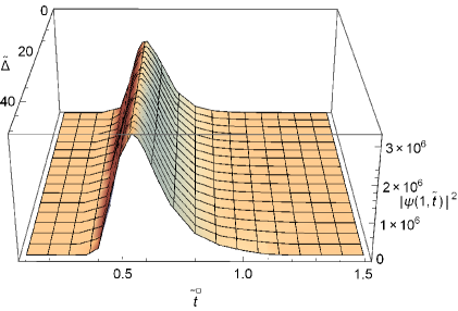
Figure 1: Probability density distribution $\left|\psi(1,\widetilde{t})\right|^{2}$ on the right-hand side of the barrier as a function of time and asymmetry parameter $\widetilde{\Delta}$ for the narrow energy distribution of the initial wave packet ($\widetilde{\sigma}=1/3$).

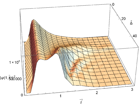
Figure 2: Probability density $\left|\psi(1,\widetilde{t})\right|^{2}$ as a function of $\widetilde{t}$ and $\widetilde{\Delta}$ for the broad energy distribution of the initial wave packet ($\widetilde{\sigma}=0.1$).

For the case of a potential well with $\widetilde{U}=-10^{2}$, we numerically evaluated $\left|\psi(\widetilde{x},\widetilde{t})\right|^{2}$ inside the well ($\widetilde{x}=0\div 1$) for the case of the broad energy distribution of the initial wave packet ($\widetilde{\sigma}=0.1$) and the asymmetry parameter $\widetilde{\Delta}=0$ and $\widetilde{\Delta}=\widetilde{E}_{\bot}/2=\left|\widetilde{U}\right|/2$. Figure 3 shows the interference pattern inside the symmetric well which differs sufficiently from the stationary square cosine type picture, given by Eq. (42) (for $\Delta=0$). It is seen that the amplitude of this pattern grows with time from zero to the maximum value (reached approximately at $\widetilde{t}=0.5$) and then again diminishes to zero, thereby showing the finite time during which a particle exists in the well region before leaving it either for the region before ($\widetilde{x}<0$) or beyond ($\widetilde{x}>1$) the well. We also see that the interference pattern of $\left|\psi(\widetilde{x},\widetilde{t})\right|^{2}$ is more structured in space and time. These changes in the probability density distribution result from the influence of the backward-moving components of the wave function $\psi_{<}(\widetilde{x},\widetilde{t})$, which is essential for the considered case of sufficient energy dispersion ($\widetilde{E}_{\bot}\widetilde{\sigma}^{2}=1$). In Fig. 4, we see the influence of the asymmetry parameter ($\widetilde{\Delta}=50$) on that probability density $\left|\psi(\widetilde{x},\widetilde{t})\right|^{2}$ inside the asymmetric well. The calculated distribution exhibits a very structured and pronouncedly nonmonotonic interference pattern in space and time compared with that displayed in Fig. 3.

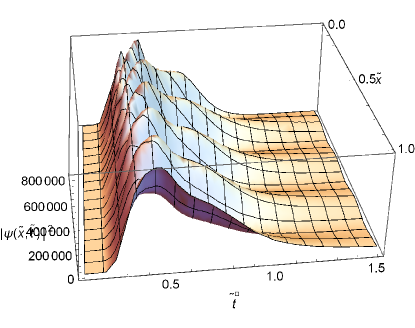
Figure 3: Probability density $\left|\psi(\widetilde{x},\widetilde{t})\right|^{2}$ inside the symmetric well ($\widetilde{\Delta}=0$) for the broad energy distribution of the initial wave packet ($\widetilde{\sigma}=0.1$).

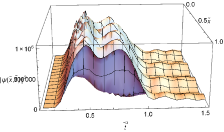
Figure 4: Probability density $\left|\psi(\widetilde{x},\widetilde{t})\right|^{2}$ inside the asymmetric well ($\widetilde{\Delta}=50$) for $\widetilde{\sigma}=0.1$.

5 Dwell time

For a finite spatial interval, the so-called dwell time, i.e. the average time spent in this interval by a particle described by the packet $\psi(x,t)$, is customarily used. The dwell time in the potential region ($0,d$) can be defined in the three-dimensional case for the potential (1) as

$$\tau(0,d)=\lim_{t-t_{0}\rightarrow\infty}{\displaystyle\int\limits_{t_{0}}^{t}}dt{\displaystyle\int\limits_{0}^{d}}dx\int d\mathbf{\rho}\left|\psi(x,\mathbf{\rho,}t)\right|^{2}.$$ (44)

Substituting the third and fourth lines of (24) into the definition (44), we obtain for the initial wave packet (27)

$$\tau(0,d) =\tau_{>}(0,d)+\tau_{<}(0,d)+2\operatorname{Re}\tau_{><}(0,d),$$

$$\tau_{>}(0,d) ={\displaystyle\int\limits_{0}^{\infty}}dE{\displaystyle\int\limits_{0}^{d}}dx\left|\frac{\varphi(x,E)}{\sqrt{v_{u}(E)}}\psi_{>}(E)\right|^{2},\tau_{<}(0,d)={\displaystyle\int\limits_{0}^{\infty}}dE{\displaystyle\int\limits_{0}^{d}}dx\left|\frac{\varphi(x,E)}{\sqrt{v_{u}(E)}}\psi_{<}(E)\right|^{2},$$

$$\tau_{><}(0,d) ={\displaystyle\int\limits_{0}^{\infty}}dE{\displaystyle\int\limits_{0}^{d}}dx\left[\frac{\varphi(x,E)}{\sqrt{v_{u}(E)}}\right]^{2}\psi_{>}(E)\psi_{<}^{\ast}(E),$$

$$\varphi(x,E) =t^{\prime}(E)e^{ik_{u}x}+r^{\prime}(E)e^{-ik_{u}x},$$ (45)

where the functions $\psi_{>(<)}(E)$ are defined by (28) and the equality (29) is taken into account.

We see that, again, the dwell time is determined by the forward- and backward-moving components of the initial wave packet as well as their interference. The entire range of energy ($0\div\infty$) contributes to the dwell time. It is not difficult to get from (45), (17) and (21) that the forward- and backward-moving components of the dwell time are

$$\tau_{>(<)}(0,d)={\displaystyle\int\limits_{0}^{\infty}}dE\tau_{>(<)}(E;d).$$ (46)

The per unit energy interval energy-dependent dwell time $\tau_{>(<)}(E;d)$ caused by the forward- (backward-) moving component of the initial wave packet $\psi_{>(<)}(E)$ is for $E>\Delta$ ($k_{\Delta}=\sqrt{2m(E-\Delta)/\hbar^{2}}$ is real)

$$\tau_{>(<)}(E;d) =t(E;d)\left|\psi_{>(<)}(E)\right|^{2},$$

$$t(E;d) =\frac{k}{v_{u}}\frac{2k_{u}d(k_{u}^{2}+k_{\Delta}^{2})-K_{0}^{2}\sin(2k_{u}d)}{(k+k_{\Delta})^{2}k_{u}^{2}+k_{0}^{2}K_{0}^{2}\sin^{2}(k_{u}d)},E>\Delta\geq 0,$$ (47)

where $K_{0}^{2}=k_{\Delta}^{2}-k_{u}^{2}=\frac{2m}{\hbar^{2}}(U-\Delta)$, $k_{0}^{2}=k^{2}-k_{u}^{2}=\frac{2m}{\hbar^{2}}U$. For $E<\Delta$, $\Delta\geq 0$ ($k_{\Delta}=i\overline{k}_{\Delta}$, $\overline{k}_{\Delta}=\sqrt{2m(\Delta-E)/\hbar^{2}}$)

$$t(E;d)=\frac{k}{v_{u}}\frac{2k_{u}d(k_{u}^{2}+\overline{k}_{\Delta}^{2})-\overline{K}_{0}^{2}\sin(2k_{u}d)+4k_{u}\overline{k}_{\Delta}\sin^{2}(k_{u}d)}{(k+\overline{k}_{\Delta})^{2}k_{u}^{2}+k_{0}^{2}\overline{K}_{0}^{2}\sin^{2}(k_{u}d)+k_{0}^{2}k_{u}\overline{k}_{\Delta}\sin(2k_{u}d)},E<\Delta,\Delta>0,$$ (48)

where $\overline{K}_{0}^{2}=\overline{k}_{\Delta}^{2}-k_{u}^{2}=\frac{2m}{\hbar^{2}}(U+\Delta-2E)$. Both Eq. (47) and Eq. (48) are valid for $k_{u}$ real as well as for the imaginary $k_{u}=i\overline{k}_{u}$, $\overline{k}_{u}=\sqrt{2m(U-E)/\hbar^{2}}$ when $E<U$ (barrier). Note that $\psi_{>(<)}(E)$ has the dimensionality of the inverse square root of energy (see (28)), and thus the expression for $t(E;d)$ has the dimensionality of time and represents the generalization of the energy-dependent dwell time obtained earlier by Buttiker [23] to the case of the asymmetric rectangular potential (1) (if $\Delta=0$, Eq. (47) reduces to the Buttiker result).

The per unit energy interval interference dwell time which follows from (45) can be written as

$$\tau_{><}(E;d) =\operatorname{Re}\left\{\frac{k}{v_{u}}\frac{(k_{u}^{2}+k_{\Delta}^{2})\sin(2k_{u}d)+2(k_{u}^{2}-k_{\Delta}^{2})k_{u}d-4ik_{u}k_{\Delta}\sin^{2}(k_{u}d)}{\left[i(kk_{\Delta}+k_{u}^{2})\sin(k_{u}d)-k_{u}(k+k_{\Delta})\cos(k_{u}d)\right]^{2}}\psi_{>}(E)\psi_{<}^{\ast}(E)\right\},$$

$$\operatorname{Re}\tau_{><}(0,d) ={\textstyle\int\limits_{0}^{\infty}}dE\tau_{><}(E;d).$$ (49)

Note that Eq. (49) holds for both $k_{u}$ real ($E>U$) and imaginary $k_{u}=i\overline{k}_{u}$ ($E<U$), as well as for both the real $k_{\Delta}$ ($E>\Delta$) and imaginary $k_{\Delta}=i\overline{k}_{\Delta}$ ($E<\Delta$).

We see that the total per unit energy dwell time

$$\tau(E;d)=t(E;d)\left[\left|\psi_{>}(E)\right|^{2}+\left|\psi_{<}(E)\right|^{2}\right]+2\tau_{><}(E;d),\tau(0,d)=\int\limits_{0}^{\infty}\tau(E;d)dE$$ (50)

is generally defined by both the forward- and backward-moving components of the initial wave packet as well as their interference. For the resonance energies satisfying the condition $k_{u}d=\pi n$ ($n$ is integer, $k_{u}$ is real), taking place in the cases of $U<0$ and $U>0$ (when $E>U$), Eqs. (47) -(50) reduce, e.g. for $k_{\Delta}$ real ($E\geq\Delta$), to

$$\tau(E;d)=\frac{d}{v}\left\{\frac{2k^{2}(k_{u}^{2}+k_{\Delta}^{2})}{k_{u}^{2}(k+k_{\Delta})^{2}}\left[\left|\psi_{>}(E)\right|^{2}+\left|\psi_{<}(E)\right|^{2}\right]+4\operatorname{Re}\frac{k^{2}(k_{u}^{2}-k_{\Delta}^{2})}{k_{u}^{2}(k+k_{\Delta})^{2}}\left[\psi_{>}(E)\psi_{<}^{\ast}(E)\right]\right\},$$ (51)

where $d/v(E)$ is the time that it takes for a particle with the energy $E$ to propagate through the spatial range $d$ in the absence of a potential. Thus, the expression in the curly brackets in (51) shows the difference between the dwell time in the range of the potential and the ”free” dwell time $d/v(E)$.

From the above it follows that, generally, the dwell time depends on the energy spectrum of the initial wave packet $\psi_{>(<)}(E)$ and cannot be realistically defined, e.g., simply by $t(E;d)$ (47) or (48). Further, we will use $\psi_{>(<)}(E)$ (28), defined for the Gaussian initial wave packet, and shift to the dimensionless variables defined in the previous section. As a result, we obtain from Eqs. (47) - (50)

$$\tau(0,d) ={\displaystyle\int\limits_{0}^{\infty}}d\widetilde{E}\widetilde{\tau}(\widetilde{E};d),\widetilde{\tau}(\widetilde{E};d)=\widetilde{\tau}_{>}(\widetilde{E};d)+\widetilde{\tau}_{<}(\widetilde{E};d)+\widetilde{\tau}_{><}(\widetilde{E};d),$$

$$\widetilde{\tau}_{>}(\widetilde{E};d)+\widetilde{\tau}_{<}(\widetilde{E};d) =\frac{t_{d}\widetilde{\sigma}}{2\sqrt{2\pi}}\frac{1}{\sqrt{\widetilde{E}-\widetilde{U}}}\frac{2\sqrt{\widetilde{E}-\widetilde{U}}(2\widetilde{E}-\widetilde{U}-\widetilde{\Delta})-(\widetilde{U}-\widetilde{\Delta})\sin(2\sqrt{\widetilde{E}-\widetilde{U}})}{(\sqrt{\widetilde{E}}+\sqrt{\widetilde{E}-\widetilde{\Delta}})^{2}(\widetilde{E}-\widetilde{U})+\widetilde{U}(\widetilde{U}-\widetilde{\Delta})\sin^{2}(\sqrt{\widetilde{E}-\widetilde{U}})}$$

$$\times\left\{\exp[-2(\sqrt{\widetilde{E}_{\bot}}-\sqrt{\widetilde{E}})^{2}\widetilde{\sigma}^{2}]+\exp[-2(\sqrt{\widetilde{E}_{\bot}}+\sqrt{\widetilde{E}})^{2}\widetilde{\sigma}^{2}]\right\},\widetilde{E}>\widetilde{\Delta}\geq 0,$$

$$\widetilde{\tau}_{><}(\widetilde{E};d) =\frac{t_{d}\widetilde{\sigma}}{\sqrt{2\pi}}\times$$

$$\operatorname{Re}\frac{1}{\sqrt{\widetilde{E}-\widetilde{U}}}\frac{(2\widetilde{E}-\widetilde{U}-\widetilde{\Delta})\sin(2\sqrt{\widetilde{E}-\widetilde{U}})+2\sqrt{\widetilde{E}-\widetilde{U}}(\widetilde{\Delta}-\widetilde{U})-4i\sqrt{\widetilde{E}-\widetilde{\Delta}}\sqrt{\widetilde{E}-\widetilde{U}}\sin^{2}(\sqrt{\widetilde{E}-\widetilde{U}})}{[i(\sqrt{\widetilde{E}}\sqrt{\widetilde{E}-\widetilde{\Delta}}+\widetilde{E}-\widetilde{U})\sin(\sqrt{\widetilde{E}-\widetilde{U}})-(\sqrt{\widetilde{E}}+\sqrt{\widetilde{E}-\widetilde{\Delta}})\sqrt{\widetilde{E}-\widetilde{U}}\cos(\sqrt{\widetilde{E}-\widetilde{U}})]^{2}}e^{-2i\sqrt{\widetilde{E}}\widetilde{x}_{i}}$$

$$\times\exp[-(\sqrt{\widetilde{E}_{\bot}}-\sqrt{\widetilde{E}})^{2}\widetilde{\sigma}^{2}]\exp[-(\sqrt{\widetilde{E}_{\bot}}+\sqrt{\widetilde{E}})^{2}\widetilde{\sigma}^{2}],$$ (52)

where the characteristic time $t_{d}/2=\hbar/2E_{d}=\frac{d}{v(E)}\sqrt{\widetilde{E}}=\frac{d}{v(E_{\bot})}\sqrt{\widetilde{E}_{\bot}}$, i.e. it is the time spent in the region of the potential width $d$ by a ”free” particle with the energy $E=E_{d}$ ($\widetilde{E}=1$), and thus $\widetilde{\tau}(\widetilde{E};d)$ has the dimensionality of time (for brevity, we do not show Eq. (48) in the dimensionless variables). The relative contribution of the forward- (backward-) moving components $\widetilde{\tau}_{>(<)}(\widetilde{E};d)$ and interference term $\widetilde{\tau}_{><}(\widetilde{E};d)$ to the dwell time $\tau(0,d)$ (52) depends on the value of the parameter $\widetilde{E}_{i}\widetilde{\sigma}^{2}$. If the second inequality (39) is satisfied, i.e., $\widetilde{E}_{\bot}\widetilde{\sigma}^{2}\gg 1$, the contribution of the backward-moving and interference terms to the dwell time (52) is much smaller than that of the forward-moving term $\widetilde{\tau}_{>}(\widetilde{E};d)$, and, therefore, the former terms may be ignored in the first approximation in the limit given by (39). Moreover, the integral of $\widetilde{\tau}_{>}(\widetilde{E};d)$ over $\widetilde{E}$ can be asymptotically estimated due to the sharp maximum of the integrand at $\widetilde{E}=\widetilde{E}_{\bot}$. The result is

$$\tau(0,d) \sim\tau_{>}(0,d)=\frac{d}{v(E_{\bot})}\frac{\widetilde{E}_{\bot}}{\sqrt{\widetilde{E}_{\bot}-\widetilde{U}}}\frac{2\sqrt{\widetilde{E}_{\bot}-\widetilde{U}}(2\widetilde{E}_{\bot}-\widetilde{U}-\widetilde{\Delta})-(\widetilde{U}-\widetilde{\Delta})\sin(2\sqrt{\widetilde{E}_{\bot}-\widetilde{U}})}{(\sqrt{\widetilde{E}_{\bot}}+\sqrt{\widetilde{E}_{\bot}-\widetilde{\Delta}})^{2}(\widetilde{E}_{\bot}-\widetilde{U})+\widetilde{U}(\widetilde{U}-\widetilde{\Delta})\sin^{2}(\sqrt{\widetilde{E}_{\bot}-\widetilde{U}})},$$

$$\widetilde{E}_{\bot} >\widetilde{\Delta}\geq 0,$$ (53)

which coincides with Eq. (47) for $t(E_{\bot};d)$ written in the dimensionless variables. It should be stressed that this result represents only the first term of the asymptotic expansion of ${\displaystyle\int\limits_{0}^{\infty}}d\widetilde{E}\tau_{>}(\widetilde{E};d)$ with a small value of the parameter $1/\widetilde{E}_{\bot}\widetilde{\sigma}^{2}$, i.e. for an initial wave packet characterized by an extra narrow momentum distribution.

For the resonance energies satisfying the condition $k_{u}d=\pi n$ ($n$ is integer, $n\neq 0$, $k_{u}$ is real), which reads in the dimensionless variables as $\widetilde{E}_{\bot}-\widetilde{U}=\pi^{2}n^{2}$, the relative to the ”free” dwell time $d/v(E_{\bot})$ expression (53) reduces to

$$\tau_{>}^{r}(0,d)v(E_{\bot})/d=\frac{2\widetilde{E}_{\bot}(2\widetilde{E}_{\bot}-\widetilde{U}-\widetilde{\Delta})}{(\sqrt{\widetilde{E}_{\bot}}+\sqrt{\widetilde{E}_{\bot}-\widetilde{\Delta}})^{2}(\widetilde{E}_{\bot}-\widetilde{U})}=\frac{2\widetilde{E}_{\bot}(\widetilde{E}_{\bot}-\widetilde{\Delta}+\pi^{2}n^{2})}{(\sqrt{\widetilde{E}_{\bot}}+\sqrt{\widetilde{E}_{\bot}-\widetilde{\Delta}})^{2}\pi^{2}n^{2}}.$$ (54)

At $\widetilde{U}<0$ (dwell), the inequality $\left|\widetilde{U}\right|=\pi^{2}n^{2}-\widetilde{E}_{\bot}>0$ should be satisfied ($n$ is bottom-limited), and when $\pi^{2}n^{2}\gg>\widetilde{E}_{\bot}>\widetilde{E}_{\bot}-\widetilde{\Delta}\geq 0$, which is the case for large enough $\left|\widetilde{U}\right|$, the asymptotic relative resonant dwell time (54) approaches $2\widetilde{E}_{\bot}/(\sqrt{\widetilde{E}_{\bot}}+\sqrt{\widetilde{E}_{\bot}-\widetilde{\Delta}})^{2}$. This value is greater than $1/2$, to which the values of the high order resonances of the dwell time reduce for a symmetric potential ($\widetilde{\Delta}=0$). Thus, the greater the asymmetry parameter $\Delta$, the greater the amplitudes of the dwell time resonances. For $\widetilde{U}>0$ (barrier), the condition $\widetilde{U}=\widetilde{E}_{\bot}-\pi^{2}n^{2}>0$ should hold ($\widetilde{E}_{\bot}>\widetilde{U}$, $n$ is restricted to the small values defined by $\widetilde{E}_{\bot}$), and at $\pi^{2}n^{2}\ll\widetilde{E}_{\bot}-\widetilde{\Delta}<\widetilde{E}_{\bot}$ the dwell time (54) behaves as $2\widetilde{E}_{\bot}(\widetilde{E}_{\bot}-\widetilde{\Delta})/(\sqrt{\widetilde{E}_{\bot}}+\sqrt{\widetilde{E}_{\bot}-\widetilde{\Delta}})^{2}\pi^{2}n^{2}$.

If $\widetilde{E}_{\bot}-\widetilde{U}\rightarrow 0$ (reverse points in classical physics), which can happen only at $\widetilde{U}>0$, the asymptotic relative dwell time $\tau_{>}(0,d)v(E_{\bot})/d$ (53) reduces to

$$\tau_{>}(0,d)v(E_{\bot})/d=\frac{4\widetilde{E}_{\bot}}{(\sqrt{\widetilde{E}_{\bot}}+\sqrt{\widetilde{E}_{\bot}-\widetilde{\Delta}})^{2}+\widetilde{U}(\widetilde{U}-\widetilde{\Delta})}>\frac{4\widetilde{E}_{\bot}}{4\widetilde{E}_{\bot}+\widetilde{U}^{2}}<1,\widetilde{E}_{\bot}-\widetilde{U}\rightarrow 0,$$ (55)

where the value $4\widetilde{E}_{\bot}/(4\widetilde{E}_{\bot}+\widetilde{U}^{2})$ corresponds to a symmetric potential, i.e., the dwell time (55) in the asymmetric case is larger. In particular, at $\widetilde{U}=0$ this dwell time for $\Delta>0$ is larger than the ”free” dwell time $d/v(E_{\bot})$ in the absence of a potential ($\widetilde{U}=0$, $\Delta=0$).

It is interesting to plot the dependence of the relative dwell time (53) on the amplitude of the potential $\widetilde{U}$, which changes from negative values (the well) to positive ones (the barrier), for a symmetric ($\widetilde{\Delta}=0$) and an asymmetric potential. Formula (53) is valid for both the $\widetilde{U}<0$ and $\widetilde{U}>0$ cases, and in the latter case, when $\widetilde{E}_{\bot}-\widetilde{U}<0$, Eq. (53) transfers to

$$\tau_{>}(0,d)v(E_{\bot})/d=\frac{\widetilde{E}_{\bot}}{\sqrt{\widetilde{U}-\widetilde{E}_{\bot}}}\frac{2\sqrt{\widetilde{U}-\widetilde{E}_{\bot}}(\widetilde{U}+\widetilde{\Delta}-2\widetilde{E}_{\bot})+(\widetilde{U}-\widetilde{\Delta})\sinh(2\sqrt{\widetilde{U}-\widetilde{E}_{\bot}})}{(\sqrt{\widetilde{E}_{\bot}}+\sqrt{\widetilde{E}_{\bot}-\widetilde{\Delta}})^{2}(\widetilde{U}-\widetilde{E}_{\bot})+\widetilde{U}(\widetilde{U}-\widetilde{\Delta})\sinh^{2}(\sqrt{\widetilde{U}-\widetilde{E}_{\bot}})}.$$ (56)

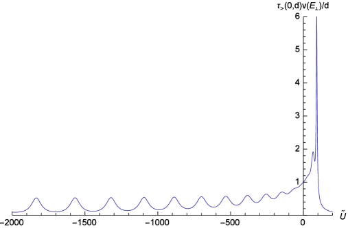
Figure 5: Dependence of the asymptotic dwell time (53) on the well/barrier symmetric potential ($\widetilde{\Delta}=0$).

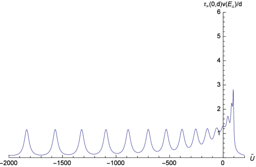
Figure 6: Dependence of the asymptotic dwell time (53) on the well/barrier asymmetric potential ($\widetilde{\Delta}=90$).

Fig. 5 shows the $\widetilde{U}$ - dependence of $\tau_{>}(0,d)v(E_{\bot})/d$ (53) for a symmetric potential ($\widetilde{\Delta}=0$) in the broad range of $\widetilde{U}=-2\times 10^{3}\div 2\times 10^{2}$ and $\widetilde{E}_{\bot}=10^{2}$. One can see the series of resonances at $\widetilde{U}<0$, the amplitudes of which approach $1/2$ for big enough $n$, $n^{2}\gg\widetilde{E}_{\bot}/\pi^{2}$, while at $\widetilde{U}>0$ there is a limited series of resonances with $n^{2}<\widetilde{E}_{\bot}/\pi^{2}$ (for $\widetilde{E}_{\bot}>\widetilde{U}$) with the larger amplitudes because a particle moves more slowly in the presence of a potential barrier than in the region of a potential well. Fig. 6 shows the same $\widetilde{U}$ - dependence of $\tau_{>}(0,d)v(E_{\bot})/d$ (53) for $\widetilde{\Delta}=90$. We see an essential increase of the resonances’ amplitudes inside the well and other details which display the influence of the potential asymmetry on the dwell time in correspondence with the analysis given above.

6 Summary

We have applied the MST to the calculation of the propagator which exactly resolves the time-dependent Schrödinger equation for a particle in the presence of a one-dimensional rectangular asymmetric well/barrier potential (1). This approach, based on the obtained effective potentials (7), (8), which are responsible for reflection from and transmission through the potential steps, is alternative to the matching procedure conventionally used for solving the stationary Schrödinger equation. The advantages of this MST approach are: A natural picture of the considered processes in terms of a particle scattering at the potential jumps (in contrast to the traditional wave point of view); The time-dependent picture of the quantum effects of particle reflection from a potential well and particle transmission through a potential barrier; The natural decomposition of the Schrödinger equation solution into the sum of the forward- and backward-moving terms (with no use of the evanescent states [3]), which takes into account that the initial wave packet, confined to a restricted spatial area and representing a particle moving towards a potential, contains both the positive and negative momentum components. Aside from being related to the fundamental issues of quantum mechanics, the obtained results can be also important for the kinetic theory of nanostructures, where the considered rectangular potential (1) is often used to model the potential profile in the magnetic nanostructures utilized, e.g., in spintronics devices.

The obtained probability density $\left|\psi(x,t)\right|^{2}$ of finding a particle in the space-time point $(x,t)$, when it initially was located in some spatial region and moved in some direction, is generally defined by the probability density corresponding to the wave component moving in this direction $\left|\psi_{>}(x,t)\right|^{2}$ as well as by the probability densities related to the backward-moving component $\left|\psi_{<}(x,t)\right|^{2}$ and the interference of both $2\operatorname{Re}[\psi_{>}(x,t)\psi_{<}^{\ast}(x,t)]$. For the case of the initial Gaussian wave packet, we have shown that the contribution of the backward-moving component to the probability density $\left|\psi(x,t)\right|^{2}$ is small when the initial packet is characterized by a narrow energy (momentum) distribution, which is characteristic of the quasi-classical approximation for a transport phenomenon. We calculated, in this case, the asymptotic time-independent values of $\left|\psi_{>}(x)\right|^{2}$ in the different spatial regions relative to the potential area. This situation (extra narrow energy distribution) actually corresponds to the stationary case with no energy dispersion. Thus, the transmission through and reflection from the potential well/barrier can be described as a function of time only when the momentum (energy) dispersion of the initial wave packet is significant (accordingly, the wave packet spatial localization is narrow). But in this case, the counterintuitive (non-classical) contribution of the backward-moving components of the wave packet should be accounted for. This rather paradoxical quantum mechanical result reveals itself in the problems connected to measuring time in quantum mechanical effects.

Using the exact result for $\left|\psi(x,t)\right|^{2}$, we have numerically plotted the time distribution of finding the particle beyond the barrier ($U>0$), $\left|\psi(1,t)\right|^{2}$ and found that, when the contribution of the backward-moving wave packet components is important (broad wave packet energy distribution), the influence of the potential asymmetry can be essential (Figs. 1,2). Plotting $\left|\psi(x,t)\right|^{2}$ in the well ($U<0$) region, we showed that the backward-moving components of the wave packet fundamentally change the probability density, when the initial wave packet is broad enough in the energy (momentum) space, and the asymmetry of the potential well adds more to the structure of this spacetime distribution (Figs. 3,4).

The obtained solution is applied to the calculation of the particle time dwell time within the potential area. Again, the forward- and backward-moving components of the obtained exact wave function contribute to the particle dwell time. For a narrow momentum distribution of the initial wave packet, the analytical asymptotic value of the main (in this case) term contributing to the dwell time in the potential region, caused by the forward-moving probability density $\left|\psi_{>}(x,t)\right|^{2}$, was obtained and plotted as a function of the potential amplitude $U$ changing from the negative (well) to the positive (barrier) values. The series resonances displayed in Figs. 5,6 show the essential influence of the potential asymmetry on the particle dwell time. These results generalize the known Buttiker results [23] for the dwell time.

References

[1]J. G. Muga, R. Sala Mayato, and I. L. Egusquiza (ed),
Time in Quantum Mechanics, Vol. 1 (Lecture Notes in Physycs, Vol.
734),Springer, Berlin (2008).
J. G. Muga, A. Ruschhaup, and A. del Campo (ed), Time in Quantum
Mechanics, Vol. 2 (Lecture Notes in Physycs, Vol. 789),Springer,
Berlin (2009).
[2]E. H. Hauge and J. A. Stovneng, Rev. Mod.Phys.,61, 917-936 (1989).
[3]A. D. Baute, I. L. Egusquiza, and J. G. Muga,
J. Phys. A: Math. Theor., 34, 4289 (2001).
[4]A. D. Baute, I. L. Egusquiza, and J. G. Muga,
Int. J. Theor. Physics., Group. Theory, Nonlinear Optics,8,
1 (2002); quant-ph/0007079.
[5]M. N. Baibich, J. M. Broto, A. Fert, F. Nguyen Van Dau, F.
Petroff, P. Etienne, G. Creuzet, A. Friederich, and J. Chazelas, Phys.
Rev. Lett.,61, 2472-2475 (1988).
[6]R. Julliere, Phys. Lett., A54, 225-226 (1975).
P. LeClair, J. S. Moodera, and R. Meservay, J. Appl. Phys.,76, 6546 (1994).
[7]A. O. Barut and I. H. Duru, Phys. Rev., A38, 5906-5909 (1988).
[8]L. S. Schulman, Phys. Rev. Lett.,49,
599-601 (1982).
[9]T. O. de Carvalho, Phys. Rev., A 47,
2562-2573 (1993).
[10]J. M. Yearsley, J. Phys. A: Math. Theor.,41, 285301 (2008).
[11]V. F. Los and A. V. Los, J. Phys. A: Math. Theor.,43, 055304 (2010).
[12]D. A. Stewart, W. H. Butler, X.-G. Zhang, and
V. F. Los, Phys. Rev., B 68, 014433 (2003).
[13]V. F. Los, Phys. Rev., B 72, 115441 (2005).
[14]V. F. Los and A. V. Los, Phys. Rev., B
77, 024410 (2008).
[15]K. A. Milton and J. Wagner, J. Phys. A: Math.
Theor.,41, 155402 (2008).
[16]V. F. Los and A. V. Los, J. Phys. A: Math.,
Theor.,44, 215301 (2011).
[17]V. F. Los and M. V. Los, J. Phys. A: Math. Theor.,45, 095302 (2012).
[18]V. F. Los and N. V. Los, Theoretical and
Mathematical Physics,177(3), 1706-1721 (2013).
[19]R. P. Feynman and A. R. Hibbs, Quantum Mechanics and
Path Integrals, MacGraw-Hill, New York (1965).
[20]E. N. Economou, Green’s Functions in Quantum
Physics, Springer, Berlin, Geidelberg, New York (1979).
[21]J. G. Muga, S. Brouard and R. F. Snider,
Phys. Rev., A46, 6075 (1992).
[22]S. Cordero and G. Garcia-Calderón, J. Phys.
A: Math. Theor.,43, 185301 (2010).