Zero-Recoil Sum Rules for $\Lambda_{b}\to\Lambda_{c}$ Form Factors

Abstract

We set up a zero recoil sum rule to constrain the form factors of the $\Lambda_{b}\to\Lambda_{c}$ transition. Our results are compared with the recent lattice calculation for these transitions. We find the same situation as in the case for $B\to D^{*}$: The lattice results practically saturate the sum rules, leaving basically no room for excited states.

I Introduction

The precise determination of the CKM matrix elements $V_{xb}$, $x=c,u$ becomes increasingly important as an input for tests of the standard model at the precision level. Although lattice QCD as well as non-lattice methods – such as QCD sum rules – have made enormous progress, we are still facing a tension between determinations of $V_{xb}$ from inclusive versus exclusive decays Kowalewski and Mannel (2014).

It is generally believed that $|V_{cb}|$ can currently be determined with the best precision via the inclusive decay $B\to X_{c}\ell\bar{\nu}$ Benson et al. (2003); Gambino and Schwanda (2014). In this case one applies an operator product expansion (OPE) in terms of local operators, which sets up and expansion for the total rate, as well as for spectral moments, in powers of $\alpha_{s}$ and $\Lambda_{\rm QCD}/m_{Q}$, $Q=b,c$. This combined expansion seems to converge rapidly, giving us confidence in the precision of the method.

On the other hand, exclusive decays also allow for a precise determination of $V_{cb}$ from the decays $B\to D^{(*)}\ell\bar{\nu}$ by extrapolating to the point of maximal momentum transfer to the leptons Kowalewski and Mannel (2014). At this point, heavy quark symmetries yield an absolute normalization of the form factors, and corrections to the form factor normalizations can be computed on the lattice Bailey et al. (2014); Lattice et al. (2015) as well as from QCD sum rules Bigi et al. (1995); Kapustin et al. (1996); Gambino et al. (2010, 2012).

The aforementioned tension between the inclusive and the exclusive determinations of $|V_{cb}|$ is driven by the lattice values for the form factor normalization for the $B\to D^{(*)}$ form factors. On the other hand, the anatomy of the $b\to c$ transition at zero recoil can be studied with zero-recoil sum rules, which hint at smaller values for the form factor normalizations and which are fully consistent with the inclusive determination. In particular, from the point of sum rules, the current lattice value would imply unexpectedly small contributions from the excited states Gambino et al. (2010, 2012).

More serious seems the problem with the determinations of $|V_{ub}|$. The inclusive determination relies on a light-cone version of the OPE leading to the corresponding heavy mass expansion Kowalewski and Mannel (2014). The hadronic input – the so called shape functions – are not well known (in particular at subleading order), and thus the resulting expansion leads to larger uncertainties compared to ones in the local OPE relevant for semileptonic $b\to c$ decays.

The exclusive determinations on $V_{ub}$ rely mainly on the channel $B\to\pi\ell\bar{\nu}$. For this decay, the form factors need to be computed either on the lattice Bailey et al. (2015) or estimated via light-cone sum rules Khodjamirian et al. (2011). Using these form factors, which turn out to be consistent between the lattice and the QCD sum rules, a value of $|V_{ub}|$ can be extracted that is about three standard deviations smaller than the inclusive one.

Since currently the exclusive determination of $V_{ub}$ rests mainly on a single channel, it is important to have an independent determination from an other channel. Since the purely leptonic decay $B\to\ell\bar{\nu}$ suffers - even for the $\tau$ lepton - from helicity suppression, the existing measurements of $B\to\tau\bar{\nu}$ are currently too imprecise to decide between the exclusive and inclusive value of $V_{ub}$. This tension has also lead to sepeculations (see e.g. Crivelin:2014zpa; Buras et al. (2011) that “new physics” is responsible for the effect, although right-handed currents have recently been excluded as an explanation Feldmann et al. (2015).

Recently the LHCb collaboration published a first measurement of the branching ratio of $\Lambda_{b}\to p\ell\bar{\nu}$ Aaij et al. (2015), which is in principle precise enough to challenge determinations based on $B\to\pi\ell\bar{\nu}$. However, this measurement is normalized to the branching ratio of $\Lambda_{b}\to\Lambda_{c}\ell\bar{\nu}$. Thus, the extraction of the ratio $|V_{ub}/V_{cb}|$ requires the form factors to be calculated for both the $\Lambda_{b}\to p$ as well as for the $\Lambda_{b}\to\Lambda_{c}$ transition. This has been done recently on the lattice for both transitions with sufficient precision in Detmold et al. (2015). Their results for the $\Lambda_{b}\to p$ transitions compare favorably with light-cone sum rule calculations Mannel and Wang (2011), but the precision of these sum rules is intrinsically limited.

In this work, we construct a zero-recoil sum rule (ZRSR) for the $\Lambda_{b}\to\Lambda_{c}$ transitions, along the same lines as for the $B\to D^{*}$ form factor, see e.g. Gambino et al. (2010). We shall investigate in this paper, if the tension present in the lattice calculation versus the zero-recoil sum rule for the mesons persists for the case of the baryons. In the next section we formulate the zero-recoil sum rule for baryons and compute the necessary OPEs to the required level of precision. We apply this method to both the axial vector and the vector current, which eventually yields constraints for a subset of the from factors that describe the $\Lambda_{b}\to\Lambda_{c}$ transitions. Finally we compare our results with the lattice values and conclude.

II Zero Recoil Sum Rule

The sum rule at zero recoil ist set up in the same way as in the case for mesons Gambino et al. (2010) by considering the forward matrix element

$$T_{\Gamma}(v\cdot q)\equiv\frac{1}{N_{\Gamma}}\int d^{4}x\,e^{-i\,(v\cdot x)\,(v\cdot q)}\langle\Lambda_{b}(P)|\mathcal{T}\big{\{}\bar{b}(x)\Gamma c(x),\,\bar{c}(0)\Gamma b(0)\big{\}}|\Lambda_{b}(P)\rangle$$ (1)

where we shall discuss two possible choices of the currents $\Gamma\otimes\Gamma$: $\gamma_{\mu}\otimes\gamma^{\mu}$ $(V\times V)$ and $\gamma_{\mu}\gamma_{5}\otimes\gamma^{\mu}\gamma_{5}$ $(A\times A)$. The normalization constants $N_{\Gamma}$ are chosen to be $N_{V}=1$ and $N_{A}=3$ for the two cases respectively. Furthermore, $P\equiv M_{\Lambda_{b}}v$ is the momentum of the $\Lambda_{b}$ baryon, from which we define the velocity $v$.

We want to set up a sum rule at the kinematical point where the charm quark also moves with the same velocity $v$ which is the point of zero-recoil transferred by the $b\to c$ transition. Thus we redefine the quark fields as

$$\bar{b}(x)=e^{+im_{b}(v\cdot x)}\bar{b}_{v}(x),\qquad\text{and}\qquad c(x)=e^{-im_{c}(v\cdot x)}c_{v}(x)\,,$$ (2)

which suggests to define the parameter $\varepsilon=m_{b}-m_{c}-(v\cdot q)$. We can then reparametrize the forward matrix element in terms of $\varepsilon$, which leads to

$$T_{\Gamma}(\varepsilon)=\frac{1}{N_{\Gamma}}\int d^{4}x\,e^{i\,\,(v\cdot x)\varepsilon}\langle\Lambda_{b}(P)|\mathcal{T}\big{\{}\bar{b}_{v}(x)\Gamma c_{v}(x)\,\bar{c}_{v}(0)\Gamma b_{v}(0)\big{\}}|\Lambda_{b}(P)\rangle$$ (3)

Since $M_{\Lambda_{b}}-M_{\Lambda_{c}}\simeq m_{b}-m_{c}$, the quantity $\varepsilon$ corresponds to the excitation energy of the intermediate charm states above the $\Lambda_{c}$. The steps leading to the sum rule are formally as in Gambino et al. (2010), however, the relevant hadronic matrix elements will be different. Along the lines of Gambino et al. (2010) we define the contour integrals

$$I_{n,\Gamma}(\varepsilon_{M})\equiv\frac{-1}{2\pi i}\oint_{|\varepsilon|=\varepsilon_{M}}\,\varepsilon^{n}\,T_{\Gamma}(\varepsilon)\,\mathrm{d}\varepsilon\,,$$ (4)

where the relevant contour is shown in figure 1.

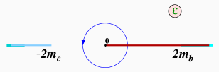
Figure 1: Integration contour for the calculation of $I_{n,\Gamma}(\varepsilon_{M})$; the radius of the contour is $\varepsilon_{M}$. Figure taken from Gambino et al. (2010).

Inserting a complete set of states, the lowest possible state is the $\Lambda_{c}$ moving with velocity $v$, the higher states will excited states of the $\Lambda_{c}$ but also non-resonant contributions such as $\Lambda_{c}\pi$ or $Dp$, where the charmed hadron moves with velocity $v$. Looking first at the integral $I_{0,\Gamma}(\varepsilon_{M})$ the lowest contribution thus is related to the square of the $\Lambda_{b}\to\Lambda_{c}$ matrix elements at zero recoil

$$F\equiv\frac{1}{N_{V}}\sum_{s^{\prime}}\langle\Lambda_{b}(v,s)|\bar{b}_{v}\gamma_{\mu}c_{v}|\Lambda_{c}(v,s^{\prime})\rangle\,\langle\Lambda_{c}(v,s^{\prime})|\bar{c}_{v}\gamma^{\mu}b_{v}|\Lambda_{b}(v,s)\rangle$$ (5)

for the vector current, and

$$G\equiv\frac{1}{N_{A}}\sum_{s^{\prime}}\langle\Lambda_{b}(v,s)|\bar{b}_{v}\gamma_{\mu}\gamma_{5}c_{v}|\Lambda_{c}(v,s^{\prime})\rangle\,\langle\Lambda_{c}(v,s^{\prime})|\bar{c}_{v}\gamma^{\mu}\gamma_{5}b_{v}|\Lambda_{b}(v,s)\rangle\\$$ (6)

for the axial-vector current.

We use the form factors for the $\Lambda_{b}\to\Lambda_{c}$ transitions in the helicity basis, which is introduced in Feldmann and Yip (2012). For the vector current they read

$$\langle\Lambda_{c}(v^{\prime},s^{\prime})|\bar{c}\gamma_{\mu}b|\Lambda_{b}(v,s)\rangle =\bar{u}_{\Lambda_{c}}(v^{\prime},s^{\prime})\left[f_{0}(w)(M_{\Lambda_{b}}-M_{\Lambda_{c}})\frac{q^{\mu}}{q^{2}}\right.$$ (7)

$$+f_{+}(w)\frac{M_{\Lambda_{b}}+M_{\Lambda_{c}}}{s_{+}}\left(M_{\Lambda_{b}}v_{\mu}+M_{\Lambda_{c}}v_{\mu}^{\prime}-(M_{\Lambda_{b}}^{2}-M_{\Lambda_{c}}^{2})\frac{q^{\mu}}{q^{2}}\right)$$ (8)

$$\left.+f_{\perp}(w)\left(\gamma_{\mu}-\frac{2M_{\Lambda_{c}}M_{\Lambda_{b}}}{s_{+}}(v_{\mu}+v_{\mu}^{\prime})\right)\right]u_{\Lambda_{b}}(v,s)\,,$$ (9)

and for the axial vector current one has

$$\langle\Lambda_{c}(v^{\prime},s^{\prime})|\bar{c}\gamma_{5}\gamma_{\mu}b|\Lambda_{b}(v,s)\rangle =-\bar{u}_{\Lambda_{c}}(v^{\prime},s^{\prime})\gamma_{5}\left[g_{0}(w)(M_{\Lambda_{b}}+M_{\Lambda_{c}})\frac{q^{\mu}}{q^{2}}\right.$$ (10)

$$+g_{+}(w)\frac{M_{\Lambda_{b}}-M_{\Lambda_{c}}}{s_{-}}\left(M_{\Lambda_{b}}v_{\mu}+M_{\Lambda_{c}}v_{\mu}^{\prime}-(M_{\Lambda_{b}}^{2}-M_{\Lambda_{c}}^{2})\frac{q^{\mu}}{q^{2}}\right)$$ (11)

$$\left.+g_{\perp}(w)\left(\gamma_{\mu}+\frac{2M_{\Lambda_{c}}M_{\Lambda_{b}}}{s_{+}}(v_{\mu}-v_{\mu}^{\prime})\right)\right]u_{\Lambda_{b}}(v,s)\,.$$ (12)

In terms of the heavy hadron velocities $v$, $v^{\prime}$ and their scalar product $w=vv^{\prime}$ one finds $q=M_{\Lambda_{b}}v-M_{\Lambda_{c}}v^{\prime}$ and $q^{2}=M_{\Lambda_{b}}^{2}+M_{\Lambda_{c}}^{2}-2M_{\Lambda_{b}}M_{\Lambda_{c}}w$. In addition, we abbreviate

$$s_{\pm}=(M_{\Lambda_{b}}\pm M_{\Lambda_{c}})^{2}-q^{2}\,.$$ (13)

With these definitions we obtain

$$F = |f_{0}(w=1)|^{2}\,,\quad\text{and}$$ (14)

$$G = \frac{1}{3}\left[2|g_{\perp}(w=1)|^{2}+|g_{+}(w=1)|^{2}\right]\,.$$ (15)

The form factors $f_{\lambda}$ and $g_{\lambda}$, $\lambda=0,+,\perp$, have been recently calculated on the lattice Detmold et al. (2015), and are published in form of a handful of parameters, including their correlation matrix. Using their results for the form factors, the authors of Detmold et al. (2015) obtain at the zero recoil point $w=1$:

$$F=0.972\pm 0.058\,,\qquad\text{and}\qquad G=0.817\pm 0.044\,.$$ (16)

In the rest of this paper we confront the above lattice results with the constraints obtained form the zero-recoil sum rule

II.1 Axial Vector Sum Rule at Zero Recoil

Parameter	mean value/ $1\sigma$ interval	unit	prior	source/comments
quark-gluon coupling and quark masses
$\alpha_{s}(m_{Z})$	0.1184 $\pm$ 0.0007	—	gaussian $@$ $68\%$	Olive et al. (2014)
$\overline{m}_{b}(\overline{m}_{b})$	4.18 $\pm$ 0.03	GeV	gaussian $@$ $68\%$	Olive et al. (2014)
$\overline{m}_{c}(\overline{m}_{c})$	1.275 $\pm$ 0.025	GeV	gaussian $@$ $68\%$	Olive et al. (2014)
hadronic matrix elements (nominal choice)
$\mu^{2}_{\pi}(1\,\text{GeV})$	0.50 $\pm$ 0.10	$\text{GeV}^{2}$	gaussian $@$ $68\%$	see eq. (24)
$\rho^{3}_{D}(1\,\text{GeV})$	0.17 $\pm$ 0.08	$\text{GeV}^{3}$	gaussian $@$ $68\%$	see eq. (25)

Table 1: Summary of the prior PDFs used in the numeric analyses. The central values lead to $m_{b}^{\text{kin}}(\mu=0.75\,\text{GeV})=4.62\,\text{GeV}$, $m_{c}^{\text{kin}}(\mu=0.75\,\text{GeV})=1.20\,\text{GeV}$, and $\alpha_{s}(\sqrt{m_{b}^{\text{kin}}m_{c}^{\text{kin}}})=0.284$.

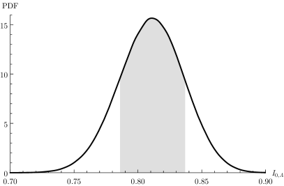
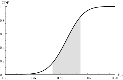
Figure 2: The result PDF (left) and the CDF (right) for the quantity $I_{0,A}$ as obtained from $10^{6}$ random samples of the paameter space. We show the central $68\%$ probability interval as the grey-shaded area.

We start the discussion with the axial vector sum rule

$$I_{0,A}(\varepsilon_{M}) =\frac{1}{N_{A}}\sum_{X_{c},\,\varepsilon\leq\varepsilon_{M}}\bra{\Lambda_{b}(v,s)}\bar{b}_{v}\gamma_{\mu}\gamma_{5}c_{v}\ket{X_{c}(v)}\bra{X_{c}(v)}\bar{c}_{v}\gamma^{\mu}\gamma_{5}b_{v}\ket{\Lambda_{b}(v,s)}$$ (17)

$$\equiv G+G_{\text{inel}}(\varepsilon_{M})$$

In the above, $G_{\text{inel}}(\varepsilon_{M})$ captures all inelastic contributions to the correlation function up to an energy $\varepsilon_{M}$, i.e., all contributions with excitation energies $0<\epsilon\leq\epsilon_{M}$. Note that both terms $G$ and $G_{\text{inel}}(\varepsilon_{M})$ are positive. We can therefore rewrite the sum rule as an upper bound for $G$:

$$G\leq I_{0,A}(\varepsilon_{M})\,.$$ (18)

The left-hand side of eq. (17) can be evaluated in the OPE Gambino et al. (2010), and one obtains

$$I_{0,A}(\epsilon_{M})=\xi^{\rm pert}_{A}(\epsilon_{M},\mu)-\Delta^{A}_{1/m^{2}}(\epsilon_{M},\mu)-\Delta^{A}_{1/m^{3}}(\epsilon_{M},\mu)+\mathcal{O}(\Lambda_{\text{had}}^{4}/m_{b}^{4},\Lambda_{\text{had}}/m_{c}^{4})$$ (19)

where the perturbative contribution is the same as for the mesonic case

$$\xi^{\rm pert}_{A}(\varepsilon_{M}=\mu=0.75\,\text{GeV})=0.970\pm 0.02\,,$$ (20)

which contains the $\alpha_{s}$ and the $\alpha_{s}^{2}$ corrections Gambino et al. (2010).

The power corrections differ from the mesonic results, since a priori the forward matrix elements for the $\Lambda_{b}$ are different from the ones for the $B$ mesons. Furthermore, for the $\Lambda$-like heavy baryons, the matrix elements of all the spin-triplet operators vanish. This is due to the fact that the light degrees of freedom do not have any angular momentum and thus cannot generate a chromomagnetic field. Hence, all matrix elements involving these operators – including $\mu^{2}_{G}(\Lambda_{b})$, $\rho^{3}_{LS}(\Lambda_{b})$ – vanish. The non-perturbative power corrections for the baryonic case therefore read

$$\Delta^{A}_{1/m^{2}} =\frac{\mu_{\pi}^{2}(\Lambda_{b})}{4}\left(\frac{1}{m_{c}^{2}}+\frac{1}{m_{b}^{2}}+\frac{2}{3m_{b}m_{c}}\right)$$ (21)

$$\Delta^{A}_{1/m^{3}} =\frac{\rho_{D}^{3}(\Lambda_{b})}{4m_{c}^{3}}+\frac{\rho_{D}^{3}(\Lambda_{b})}{12m_{b}}\left(\frac{1}{m_{c}^{2}}+\frac{3}{m_{b}^{2}}+\frac{1}{m_{b}m_{c}}\right).$$ (22)

The kinetic energy operator for the $\Lambda_{b}$ baryon has been discussed in the context of the $\Lambda_{b}$ baryon lifetime Neubert and Sachrajda (1997). Using the spin-averaged heavy meson masses one obtains up to terms of order $1/m$

$$\mu_{\pi}^{2}(B)-\mu_{\pi}^{2}(\Lambda_{b})=\frac{2m_{b}m_{c}}{m_{b}-m_{c}}\left((M_{\Lambda_{b}}-M_{\Lambda_{c}})-(\overline{M}_{B}-\overline{M}_{D})\right)(1+\mathcal{O}(1/m^{2}))\,.$$ (23)

The most recent results a of combined fit of the $B$-meson hadronic matrix elements and $V_{cb}$ to the measured lepton-energy moments in $B\to X_{c}\ell\nu$ yield $\mu_{\pi}^{2}(B)=(0.47\pm 0.07)\,\text{GeV}^{2}$ Alberti et al. (2015). Using eq. (24) this translates to

$$\mu_{\pi}^{2}(\Lambda_{b})=(0.50\pm 0.10)\,\text{GeV}^{2}\,,$$ (24)

where we increase the uncertainty to account for the lack of $1/m^{2}$ terms.

Given the small difference between the kinetic energy parameters of baryons and mesons, we use also for the Darwin term of the $\Lambda_{b}$ the same value as for the $B$-meson. The mesonic matrix element is obtained in Alberti et al. (2015); for the $\Lambda_{b}$ we use the same central value and increase the uncertainty by a factor of two,

$$\rho_{D}^{3}(\Lambda_{b})\simeq(0.17\pm 0.08)\,\text{GeV}^{3}\,.$$ (25)

Using these numbers, we obtain

$$\Delta^{A}_{1/m^{2}}(\varepsilon_{M}=\mu=0.75\,\text{GeV}) =0.108\,,$$ (26)

$$\Delta^{A}_{1/m^{3}}(\varepsilon_{M}=\mu=0.75\,\text{GeV}) =0.028\,.$$ (27)

We note that $\Delta_{1/m^{2}}$ is about $20\%$ larger than for the mesonic case, while $\Delta_{1/m^{3}}$ for the $\Lambda_{b}$ baryon yields numerically the same result as for the meson. The above results shall only be illustrative, and have been obtained for our default choice of input parameter.

For a more thorough numerical study, we use and extend EOS van Dyk et al. . This allows us to carry out a Bayesian uncertainty propagation based on Monte Carlo techniques. We choose prior probability density functions (PDFs) for all input parameters based on the principle of maximum entropy Jaynes (1957). We use Gaussian distributions throughout this work, since in all cases the mean and variance of the parameters are known. For a summary of the PDFs, see table 1. We draw $10^{6}$ random samples from $P(I_{0,A})$, the PDF of our quantitiy of interest. The result PDF and the corresponding Cumulative Probability Density Function (CDF) are shown in figure 2. For our choice of the prior PDFs, the result is a gaussian distribution to very good accuracy, with skewness $-0.08$ and excess kurtosis of $-0.04$. From the result PDF we obtain the mode and the central $68\%$ probability interval

$$I_{0,A}(\varepsilon_{M}=\mu=0.75)=0.811^{+0.025}_{-0.026}\,.$$ (28)

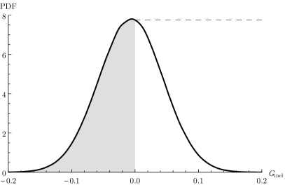
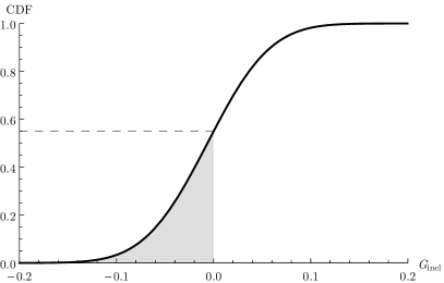
Figure 3: The result PDF (left) and CDF (right) of $G_{\text{inel}}$ as obtained from $10^{6}$ samples of both the OPE result for $I_{0,A}$ and the lattice result for $G$. The grey-shaded area shows those results with $G_{\text{inel}}<0$, which is unphysical. We find that the unphysical range of $G_{\text{inel}}$ accumulates $\sim 55\%$ probability.

Following eq. (17), we can also compute the inelastic contributions $G_{\text{inel}}$ from our nominal results for $I_{0,A}$ and the lattice results for $G$. Using $10^{6}$ samples of both quantities, we obtain the PDF and CDF for the quantity $G_{\text{inel}}$ as shown in figure 3. Again, the PDF is approximately gaussian with skewness of about $-0.01$ and excess kurtosis of about $-0.006$. We obtain the mode of the distribution and the central $68\%$ probability interval as

$$G_{\text{inel}}=-0.005^{+0.049}_{-0.052}\,.$$ (29)

Roughly $55\%$ of the samples of $G_{\text{inel}}$ turn out to be unphysical, since they are negative. Thus we conclude from this statistical analysis that the situation for the $\Lambda_{b}\to\Lambda_{c}$ is very similar as for the $B\to D^{*}$ case: The lattice results for the form factors at zero recoil saturate the corresponding zero-recoil sum rule by a very large degree, leaving almost no room for inelastic contributions. In fact, compared to the mesonic case, the situation seems to be even worse, since the central value obtained from the lattice eq. (16) exceeds the central value for our upper bound. Furthermore, for the mesonic case, one may estimate the inelastic contributions, which turn out to be sizable. This in turn implies that the zero-recoil sum rules would predict a smaller value for the form factors. Unfortunately, the estimates in the mesonic case rely on the so-called BPS limit, which cannot be used in the case of baryons. Since an estimate of the inelastic contributions in the case of the $\Lambda_{b}$ requires (possible even model dependent) input, we will not discuss this in the present paper.

II.2 Vector Sum Rule at Zero Recoil

The vector sum rule is obtained from eq. (3) by inserting $\Gamma\otimes\Gamma=\gamma_{\mu}\otimes\gamma^{\mu}$ and $N_{V}=1$,

$$I_{0,V}(\varepsilon_{M}) =\frac{1}{N_{V}}\sum_{X_{c},\,\varepsilon\leq\varepsilon_{M}}\bra{\Lambda_{b}(v,s)}\bar{b}_{v}\gamma_{\mu}c_{v}\ket{X_{c}(v)}\bra{X_{c}(v)}\bar{c}_{v}\gamma^{\mu}b_{v}\ket{\Lambda_{b}(v,s)}$$ (30)

$$\equiv F+F_{\text{inel}}(\varepsilon_{M})\,.$$

Analogous to the axial vector current, $F_{\text{inel}}(\varepsilon_{M})$ captures all inelastic contributions to the correlation function with excitation energies less than $\varepsilon_{M}$, i.e., all contributions with excitation energies $0<\epsilon\leq\epsilon_{M}$. Again, $F$ and $F_{\text{inel}}(\varepsilon_{M})$ are positive, and we can therefore rewrite the sum rule as an upper bound for the term $F$:

$$F\leq I_{0,V}(\varepsilon_{M})\,.$$ (31)

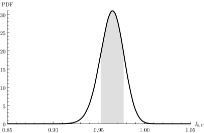
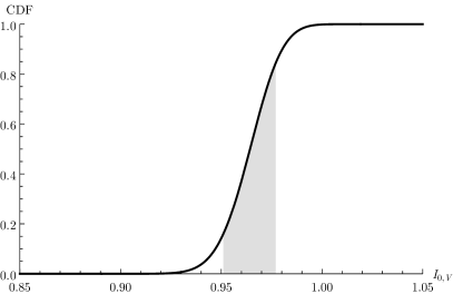
Figure 4: The result PDF (left) and CDF (right) for the quantity $I_{0,V}$ as obtained from $10^{6}$ random samples of the paameter space. We show the central $68\%$ probability interval as the grey-shaded area.

The OPE result for the left-hand side of eq. (30) reads

$$I_{0,V}(\epsilon_{M})=\xi^{\rm pert}_{V}(\epsilon_{M},\mu)-\Delta^{V}_{1/m^{2}}(\epsilon_{M},\mu)-\Delta^{V}_{1/m^{3}}(\epsilon_{M},\mu)+\mathcal{O}(\Lambda_{\text{had}}^{4}/m_{b}^{4},\Lambda_{\text{had}}/m_{c}^{4})$$ (32)

where the perturbative contribution has been evaluated to order $\alpha_{s}$ in Uraltsev (2004). For the central values of the input parameters we obtain

$$\xi^{\rm pert}_{V}(\varepsilon_{M}=\mu=0.75\,\text{GeV})=1.03^{+0.03}_{-0.01}\,,$$ (33)

where the uncertainty is estimated form a variation of the scale $0\leq\mu\leq 1.5$ GeV.

The nonperturbative corrections have been given in Bigi et al. (1995); Uraltsev (2004)

$$\Delta^{V}_{1/m^{2}} =\frac{\mu_{\pi}^{2}(\Lambda_{b})}{4}\left(\frac{1}{m_{c}}-\frac{1}{m_{b}}\right)^{2}$$ (34)

$$\Delta^{V}_{1/m^{3}} =\frac{\rho_{D}^{3}(\Lambda_{b})}{4}\left(\frac{1}{m_{c}}-\frac{1}{m_{b}}\right)^{2}\left(\frac{1}{m_{c}}+\frac{1}{m_{b}}\right)$$ (35)

and reflect the fact that the vector current is conserved in the limit $m_{b}=m_{c}$.

Inserting the central values for the hadronic matrix elements, we obtain

$$\Delta^{V}_{1/m^{2}}(\varepsilon_{M}=\mu=0.75\,\text{GeV}) =0.047\,,$$ (36)

$$\Delta^{V}_{1/m^{3}}(\varepsilon_{M}=\mu=0.75\,\text{GeV}) =0.017\,.$$ (37)

As before, these results are only meant as an illustration, and we repeat the statistical procedure as outlined in section II.1. We obtain for the mode and central $68\%$ probability interval of the result PDF for $I_{0,V}$

$$I_{0,V}(\varepsilon_{M}=\mu=0.75)=0.965\pm 0.013\,,$$ (38)

based on $10^{6}$ samples. We display the resulting PDF and CDF for $I_{0,V}$ in figure 4. We compute the inelastic contribution as well – just as before in the case of the axialvector current – and obtain

$$F_{\text{inel}}=-0.010^{+0.061}_{-0.057}\,.$$ (39)

as the mode and central uncertainty interval at $68\%$ probability; see figure 5 for the respective result PDF and CDF. We further find that $\sim 55\%$ of the drawn samples are unphysical, i.e., they show a negative inelastic contribution.

Thus our findings are qualitatively the same as in the case of the axial current: The lattice result for the scalar vector form factor $f_{0}$ at the non-recoil point again saturates the the zero-recoil sum rule to a very large degree, leaving also for this case almost no room for inelastic contributions.

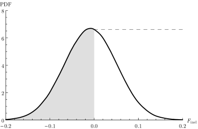
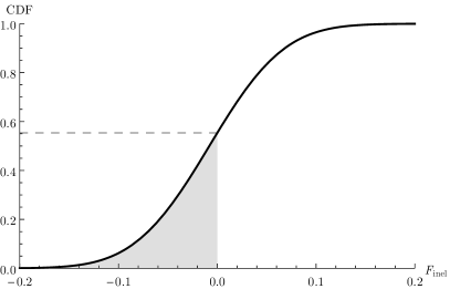
Figure 5: The PDF and the CDF of $F_{\text{inel}}$ as obtained from $10^{6}$ samples of both the OPE result for $I_{0,V}$ and the lattice result for $F$. The grey-shaded area shows those results with $F_{\text{inel}}<0$, which is unphysical. We find that the unphysical range of $F_{\text{inel}}$ accumulates $\sim 55\%$ probability.

III Discussion and Conclusion

The determination of CKM matrix elements from exclusive semileptonic decays requires reliable calculations for the form factors describing the corresponding hadronic transition. Since the form factors are genuinely non-perturbative, the only known “ab initio” calculational method is lattice QCD. The progress in this field made in the last years in the construction of efficient algorithms as well as the increasing computing power has turned lattice calculation of form factors into an indispensable tool in flavor physics.

However, despite this progress it is important to perform checks of the lattice results from “continuum” methods. One of these methods are QCD sum rules. On the one hand they are firmly rooted in QCD, on the other hand they allow for a detailed study of the “anatomy” of the results obtained e.g. for form factors. It has to be clear that a QCD sum rule can never make a precision prediction for a hadronic quantity, since the method is intrinsically limited to a level of a few ten percent.

Nevertheless, QCD sum rules can serve to validate results obtained from other methods, e.g from lattice QCD. In particular, the zero-recoil sum rules can give a hint on the sizes of the from factors at the non-recoil point; in case of the $B\to D^{*}$ transition one can combine the zero-recoil sum rule with an estimate for the inelastic contributions to actually estimate the form factor itself.

In the analysis presented here we have shown that the lattice results Detmold et al. (2015) for the $\Lambda_{b}\to\Lambda_{c}$ transition form factors saturate the zero-recoil sum rule to a large extent. In fact, we found that the central values for the lattice results exceed the sum rule’s upper bounds, leaving practically no room for any inelastic contribution. This seems to be the case for both the axial-vector as well as for the vector current.

In fact, the degree of saturation of the sum rule for the $\Lambda_{b}\to\Lambda_{c}$ seems to be higher than for the $B\to D^{*}$ transition, where the lattice value for the form factor at zero recoil still leaves room for a (too?) small inelastic contribution. Unfortunately, the inelastic contributions for the baryonic case are harder to estimate than in the mesonic case; any estimate of the inelastic contributions for the baryons would require (probably model-dependent) additional input. We leave the discussion of this to future work.