A new approach for image compression using normal matrices

Abstract

In this paper, we present methods for image compression on the basis of eigenvalue decomposition of normal matrices. The proposed methods are convenient and self-explanatory, requiring fewer and easier computations as compared to some existing methods. Through the proposed techniques, the image is transformed to the space of normal matrices. Then, the properties of spectral decomposition are dealt with to obtain compressed images. Experimental results are provided to illustrate the validity of the methods.

Keywords: Image compression, Transform, Normal matrix, Eigenvalue.

1 Introduction

Nowadays, digital images and other multimedia files can become very large in size and, therefore, occupy a lot of storage space. In addition, owing to their size, it takes more time to move them from place to place and a larger bandwidth to download and upload them on the Internet. So, digital images may pose problems if we regard the storage space as well as file sharing. To tackle this problem, image compression which deals with reducing the size of an image (or any other multimedia) file can be used. Image compression actually refers to the reduction of the amount of image data (bits) required for representing a digital image without causing any major degradation of the image quality. By eliminating redundant data and efficiently optimizing the contents of a file image, provided that as much basic meaning as possible is preserved, image compression techniques, make image files smaller and more feasible to share and store.

The study of digital image compression has a long history and has received a great deal of attention especially with respect to its many important applications. References for theory and practice of this method are [13, 14, 6, 16, 12] and [11], to name but a few.

Image compression, as well as other various fields of digital image processing, benefits from the theory of linear algebra as a helpful tool. In particular, Singular Value Decomposition (SVD) is one of the most useful tools for image compression [18, 15].

The matrix $A\in\mathbb{C}^{m\times n}$ can be written in the form of $USV^{*}$, where $U\in\mathbb{C}^{m\times m}$ and $V\in\mathbb{C}^{n\times n}$ are unitary matrices, i.e., $U^{*}U=I_{m},V^{*}V=I_{n}$, where ^∗ denotes complex conjugate transpose and $I_{n}$ is $n\times n$ identity matrix. The matrix $S$ is an $m\times n$ diagonal matrix in such a way that its nonnegative entries are ordered in a non-increasing order (see for example, Theorem 7.3.5 of [9]). With respect to the influences of singular values of $A$ in compressing an image, and considering the important point that the singular values of $A$ are the positive square roots of the eigenvalues of matrices $A^{*}A$ and $AA^{*}$, the present study concerns itself with the eigenvalue of the normal matrices $A+A^{*}$ and $A-A^{*}$ on the purpose of establishing certain techniques for image compression that are efficient, lead to desirable results and need fewer calculations.

In the next section, we briefly present some definitions and concepts about normal matrices. Section 3 consists of two subsections in which the proposed image compression methods are explained. In Section 4, the validity rates of the presented image compression schemes are investigated and compare their efficiencies by experimental results.

2 Normal matrices

In this section, we review the definition and some properties of normal matrices. See [5, 8] and the references mentioned there as the suggested sources on a series of conditions on normal matrices. In the next section, we will describe the proposed method on the basis of these presented properties.

A matrix $M\in\mathbb{C}^{n\times n}$ is called normal if $M^{*}M=MM^{*}$. Assuming $M$ as an $n$-square normal matrix, there exists an orthonormal basis of $\mathbb{C}^{n\times n}$ that consists of eigenvectors of $M$, and $M$ is unitarily diagonalizable. That is, let the scalars $\lambda_{1},\ldots,\lambda_{n}$, counted according to multiplicity, be eigenvalues of the normal matrix $M$ and let $u_{1},\ldots,u_{n}$ be its corresponding orthonormal eigenvectors. Then, the matrix $M$ can be factored as the following:

$$M=U\Lambda U^{*}=\sum\limits_{i=1}^{n}{\lambda_{i}u_{i}u_{i}^{*}},\qquad\Lambda=\mbox{diag}(\lambda_{1},\ldots,\lambda_{n}),\qquad U=[u_{1},\ldots,u_{n}],$$

where the matrix $U$ satisfies $UU^{*}=I_{n}$. Maintaining the generality, assume that eigenvalues are ordered in a non-ascending sequence of magnitude, i.e., $\left|{\lambda_{1}}\right|\geq\left|{\lambda_{2}}\right|\ldots\geq\left|{\lambda_{n}}\right|$.

It is to be noticed that, if all the elements of the matrix $M$ are real, then $M^{*}=M^{T}$, where $M^{T}$ refers to the transpose of the matrix $M$. A square matrix $M$ is called symmetric if $M=M^{T}$ and called skew-symmetric if $M=-M^{T}$. That symmetric and skew-symmetric matrices are normal is easy to see. Also, the whole set of the eigenvalues of a real symmetric matrix are real, but all the eigenvalues of a real skew-symmetric matrix are purely imaginary. A general square matrix $M$ satisfies $M=B+C$, for which the symmetric matrix $B=(M+M^{T})/2$ is called the symmetric part of $M$ and, similarly, the skew-symmetric matrix $C=(M-M^{T})/2$ is called the skew-symmetric part of $M$. As a consequence, every square matrix may be written as the sum of two normal matrices: a symmetric matrix and a skew-symmetric one. We specially use this point in the proposed image compression techniques.

3 Image compression methods

This section consists of two subsections where methods for image compression are presented using normal matrices. To this purpose, the matrix representing the image is transformed into the space of normal matrices. Next, the properties of its eigenvalue decomposition are utilized, and some less significant image data are deleted. Finally, by returning to the original space, the compressed image can be constructed.

Let $X$ be an $n\times n$ matrix to represent the image. Two distinct methods are taken into account. First, the symmetric parts of $X$ are dealt with to establish an image compression scheme. This procedure can be performed in the same way for the skew-symmetric parts of the matrix $X$. Next, another technique is explained using both symmetric and skew-symmetric parts of the matrix $X$. What is noticeable is that finding the eigenvalues and eigenvectors of a matrix requires fewer calculations than finding its singular values and singular vectors. Moreover, it is possible to calculate the eigenvalues and eigenvectors of a normal (especially symmetric or skew-symmetric) matrix by explicit formulas and, therefore, may yet again need less computation [3, 4, 7].

3.1 Image compression method using the symmetric part of $X$

In this subsection, a technique of image compression comes into focus on the basis of the eigenvalue decomposition of the symmetric parts of the matrix $X$. This can be performed in the same way for the skew-symmetric parts of $X$. It is to be noted that, for the same image, the results obtained by these two techniques (i.e. using symmetric or skew-symmetric part) may be different.

Assume $B_{X}$ as the symmetric part of the matrix $X$. The normal matrix $B_{X}$ can be factored as in the following:

$$B_{X}=U_{B_{X}}\Lambda_{B_{X}}U_{B_{X}}^{*}=\sum\limits_{i=1}^{n}{\lambda_{B_{X,i}}u_{B_{X,i}}u_{B_{X,i}}^{*}},\qquad\Lambda_{B_{X}}=\mbox{diag}(\lambda_{B_{X,1}},\ldots,\lambda_{B_{X,n}}),$$

Now, bearing in mind that the eigenvalues are sequenced in a non-ascending order of magnitude, compress the symmetric part of the image by wiping off the small enough eigenvalues of $B_{X}$. If $k$ of the larger eigenvalues remains, then there is

$$\tilde{B}_{X}=\sum\limits_{i=1}^{k}{\lambda_{B_{X,i}}u_{B_{X,i}}u_{B_{X,i}}^{*}}\;;\qquad k\leq n,$$ (1)

where the total storage for $\tilde{B}_{X}$ is $k(n+1)$. Here comes the stage of reconstructing the compressed image $\tilde{X}$ from its symmetric part. To this purpose, all the elements located above the main diagonal of the matrix $X$ are needed, and this calls for ${{n\left({n-1}\right)}}/2$ storage spaces. Because $\tilde{X}$ can be considered as an acceptable approximation of $X$, let us take all the elements above the main diagonal of $\tilde{X}$ as the elements of $X$. Obviously, the elements located below the main diagonal of the matrix $\tilde{X}^{T}$ should be determined too. In addition, it is inferred from the fact $2\tilde{B}_{X}=\tilde{X}+\tilde{X}^{T}$ that the elements located below the main diagonal of $\tilde{X}$ can be obtained by subtracting the elements below the main diagonal of $2\tilde{B}_{X}$ from the elements of $\tilde{X}^{T}$ . See the following equation where $"\checkmark"$ and $"\times"$ denote the given and unknown entries, respectively.

$$2\tilde{B}_{X}=\mathop{\left[{\begin{array}[]{*{20}c}\times&{}\hfil&\checkmark\\ {}\hfil&\ddots&{}\hfil\\ \times&{}\hfil&\times\\ \end{array}}\right]}\limits_{\tilde{X}}+\mathop{\left[{\begin{array}[]{*{20}c}\times&{}\hfil&\times\\ {}\hfil&\ddots&{}\hfil\\ \checkmark&{}\hfil&\times\\ \end{array}}\right]}\limits_{\tilde{X}^{T}}.$$

It is clear that the main diagonal elements of $\tilde{X}$ are the same as those on the main diagonal of $\tilde{B}_{X}$. It is also to be noted that, by this procedure, only the elements located below the main diagonal of $X$ are modified, and its other elements are remain untouched.

Moreover, to reconstruct the compressed image $\tilde{X}$, the elements located below the main diagonal of $X$ may be reserved instead of those above the main diagonal, and then a procedure similar to what has been performed newly is to be followed. Indeed, $X$ can be partitioned into several segments, and those segments may be reserved provided that $\tilde{X}$ is reconstructed. This may be useful specially when some segments of the image have more significance or unchanging (or uncompressing) some partitions of the image is desirable during the image compression.

Finally, it should be pointed out that reconstruction of the compressed image $\tilde{X}$ requires $\left(k(n+1)+\frac{{n\left({n-1}\right)}}{2}\right)$ storage spaces when the symmetric part of $X$ is dealt with. However, if the skew-symmetric part of $X$ is concerned, the diagonal elements of the $\tilde{X}$ cannot be obtained from $\tilde{B}_{X}$ and, therefore, they must be reserved. Reconstructing the compressed image $\tilde{X}$, thus, requires $\left(k(n+1)+\frac{{n\left({n+1}\right)}}{2}\right)$ storage spaces when the skew-symmetric part of $X$ is considered for the image compression method. In the next subsection, another image compression technique is provided, for which reconstructing the compressed image demands fewer storage spaces.

3.2 Image compression method using both symmetric and skew-symmetric parts of $X$

The previous subsection introduced an image compression scheme dealing with almost half of an image. By that technique, more than half of the elements of the image remained unchanged. This may be of some usages and advantages. Compressed images obtained by the presented method have a high quality. However, compressing of just half of the original image may cause the method to lose its reliability as compared to some other image compression schemes. To tackle this problem, a new method is presented here about both symmetric and skew-symmetric parts of the matrix $X$ in order to compress the image all over. This new image compression technique is found to be of a remarkably high reliability.

As previously mentioned, every matrix equals the sum of its symmetric and skew-symmetric parts. To establish the new method, with the definition of $B_{X}$, borne in mind, $C_{X}$ is used to represent the skew-symmetric part of $X$. The matrix $C_{X}$ can be written as follows:

$$C_{X}=U_{C_{X}}\Lambda_{C_{X}}U_{C_{X}}^{*}=\sum\limits_{i=1}^{n}{\lambda_{C_{X,i}}u_{C_{X,i}}u_{C_{X,i}}^{*}},\qquad\Lambda_{C_{X}}=\mbox{diag}(\lambda_{C_{X,1}},\ldots,\lambda_{C_{X,n}}),$$

With respect to the method described in the previous subsection, for an integer $k\leq n$, set

$$\tilde{C}_{X}=\sum\limits_{i=1}^{k}{\lambda_{B_{X,i}}u_{C_{X,i}}u_{C_{X,i}}^{*}},$$ (2)

Through (1) and (2), the compressed image $\mathcal{X}$ will be $\mathcal{X}=\tilde{B}_{X}+\tilde{C}_{X}.$ As in the case of reserving the matrix $\tilde{B}_{X}$, $k(n+1)$ storage spaces are required for saving the matrix $\tilde{C}_{X}$. As a result, the total storage requirement for $\mathcal{X}$ is $2k(n+1)$.

4 Experimental results

In this section, the validity and the influence of the proposed image compression method are examined. Let us note that the ideas presented in this paper, can readily be used to establish a block-based compression scheme. This scheme concerns dividing of an image into non-overlapping blocks and compressing of each block.

The Peak Signal to Noise Ratio (PSNR) is calculated to measure the quality of the compressed image. In the case of gray scale images of size $M\times N$, whose pixels are represented with 8 bits, PSNR is computed as follows:

$$PSNR=10\log_{10}^{\frac{{255^{2}}}{{MSE}}};\qquad MSE=\frac{1}{{MN}}\sum\limits_{i,j}{\left|{X_{i,j}-\mathcal{X}_{i,j}}\right|^{2}},$$

where $X_{i,j}$ and $\mathcal{X}_{i,j}$ refer to the elements of the original and the compressed images respectively. In the above relationship, MSE stands for the Mean Square Error between the original image and the compressed image pixels. In addition, Compression Ratio (CR) may be calculated as an important index to evaluate how much of an image is compressed. CR is the amount of bits in the original image divided by the amount of bits in the compressed image; that is,

$$\mbox{CR}=\frac{\mbox{Original Image Size}}{\mbox{Compressed Image Size}}.$$

For the sake of simplicity, Method #1 and Method #2 are branded as image compression techniques which use the symmetric and the skew-symmetric parts of the matrix representing the image, in the image compression schemes, respectively. In addition, let Method #3 denominate the image compression technique described in Subsection 3.2 and let Method #4 stand for the image compression method using SVD. Consequently, the following relationships emerge for CR of these methods:

$$CR_{Method\#1}=\frac{{n^{2}}}{{\left({k(n+1)+\frac{{n(n-1)}}{2}}\right)}},\qquad CR_{Method\#2}=\frac{{n^{2}}}{{\left({k(n+1)+\frac{{n(n+1)}}{2}}\right)}},$$

$$CR_{Method\#3}=\frac{{n^{2}}}{{2k(n+1)}},\hskip 25.6073pt\mbox{and}\hskip 25.6073ptCR_{Method\#4}=\frac{{n^{2}}}{{k(2n+1)}}.$$

In the experiments conducted in this study, three $512\times 512$ gray scale images were considered, including (a) Lena, (b) Baboon and (c) Gold hill presented in Fig 1. The PSNR results are shown in Tables 1, 2 and 3, for some integer values of $k$, for images Lena, Baboon and Gold hill, respectively. Also, the CR results are given in Table 4 for a $512\times 512$ image. The results obtained by these techniques are compared to those achieved by Method #4 in our tables. Furthermore, Figures 2 and 3 show the compressed image Lena obtained by the proposed techniques as well as image compression method using SVD, Method #4, for $k=50$ and $k=100$, respectively.

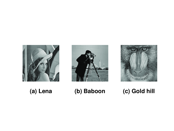
Fig 1: Original Images

Table 1: PSNR results for Lena

$k$	Method#1	Method#2	Method#3	Method #4
10	21.7012	22.3391	22.0050	22.4065
20	24.8722	25.0305	24.9462	25.2937
30	26.8832	27.0315	26.9531	27.2243
40	28.3856	28.5746	28.4751	28.7927
50	29.7358	29.9001	29.8129	30.1761
75	32.5608	32.8031	32.6763	33.1093
100	35.0504	35.1668	35.1047	35.6641
150	39.2993	39.2955	39.2938	39.8988

Table 2: PSNR results for Baboon

$k$	Method#1	Method#2	Method#3	Method #4
10	19.7071	19.7560	19.7270	19.8493
20	20.6441	20.7135	20.6736	20.7510
30	21.3880	21.4336	21.4053	21.5203
40	22.0773	22.1009	22.0842	22.2453
50	22.7319	22.7355	22.7286	22.9306
75	24.2968	24.3207	24.3042	24.5787
100	25.8111	25.7420	25.7723	26.1761
150	28.7678	28.6798	28.7194	29.3173

Table 3: PSNR results for Gold hill

$k$	Method#1	Method#2	Method#3	Method #4
10	23.9494	23.9081	23.9223	24.1270
20	26.3107	26.2783	26.2884	26.6046
30	27.8179	27.8131	27.8092	28.1740
40	29.0044	28.9622	28.9768	29.3828
50	30.0126	29.9975	29.9978	30.4103
75	32.1111	32.1537	32.1254	32.6597
100	33.9084	33.8903	33.8927	34.5614
150	37.0963	37.0375	37.0626	37.8911

Table 4: CR results for an image of size $512\times 512$

$k$	Method#1	Method#2	Method#3	Method #4
10	1.9283	1.9211	25.5501	25.5750
20	1.8582	1.8515	12.7750	12.7875
30	1.7930	1.7867	8.5167	8.5250
40	1.7322	1.7264	6.3875	6.3938
50	1.6754	1.6699	5.1100	5.1150
75	1.5485	1.5438	3.4067	3.4100
100	1.4394	1.4354	2.5550	2.5575
150	1.2617	1.2586	1.7033	1.7050

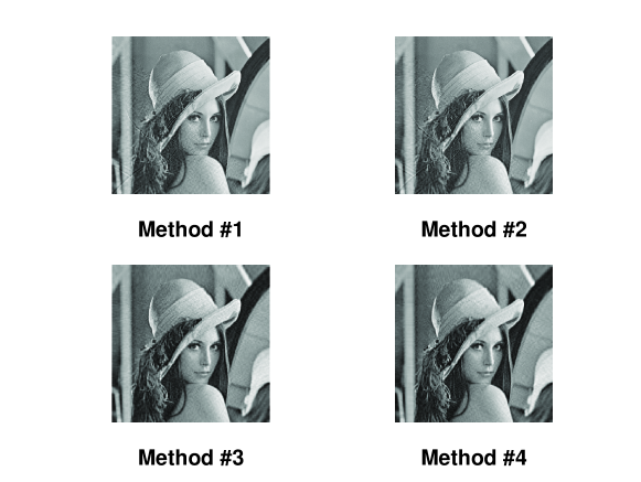
Fig 2: Compressed image Lena for $k=50$.

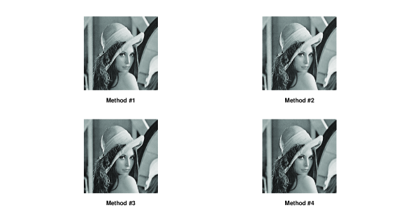
Fig 3: Compressed image Lena for $k=100$.

5 Conclusion

In this paper, the eigenvalue decomposition of symmetric and skew-symmetric matrices, as two important kinds of normal matrices, and their properties were applied to obtain image compression schemes. The proposed method is straightforward and uncomplicated ones requiring clear and fewer computations as compared to some exiting methods. This image compression method is the first one ever introduced and concerns the symmetric part of an image, which can also be applicable in the case of the skew-symmetric part of the image. The method is capable of keeping half (or some selected segments) of an image unchanged, and this feature may be of some usages. However, as observed in this study, just half of the original image could be changed, which causes the compressed image to lose its reliability. This is what makes the technique different from some other image compression techniques. Hence, the second image compression scheme using both symmetric and skew-symmetric parts of the original image was proposed. The experimental results show the high reliability of this method. Finally, it is to be pointed out that the proposed method can be used to devise block-based compression techniques.

References

- [1]
- [2] T.J. Chen, K. Chuang, A Pseudo Lossless Image Compression Method, IEEE, pp. 610–615, (2010).
- [3] J. Cullum, R.A. Willoughby, Computing eigenvalues of very large symmetric matrices An implementation of a Lanczos algorithm with no re-orthogonalization, Journal of Computational Physics, 44 (1981) 329–358.
- [4] E.R. Davidson, The iterative calculation of a few of the lowest eigenvalues and corresponding eigenvectors of large real-symmetric matrices, Journal of Computational Physics, 17 (1975) 87–94.
- [5] L. Elsner, Kh.D. Ikramov, Normal matrices: an update, Linear Algebra and its Applications, 285 (1998) 291–303.
- [6] U. Grasemann, R. Miikkulainen, Effective Image Compression using Evolved Wavelets,.ACM, pp. 1961–1968, (2005).
- [7] R.T. Gregory, Computing eigenvalues and eigenvectors of a symmetric matrix on the ILLIAC, Mathematical Tables and Other Aids to Computation, 7 (1953) pp. 215–220.
- [8] R. Grone, C.R. Johnson, E.M. Sa, H. Wolkowicz, Normal matrices, Linear Algebra and its Applications, 87 (1987) 213–225.
- [9] R.A. Horn, C.R. Johnson, Matrix Analysis, Cambridge University Press, Cambridge, 1985.
- [10] Jia, Yin-jie, Peng-fei Xu, Xu-ming Pei., An Investigation of Image Compression Using Block Singular Value Decomposition., Communications and Information Processing. Springer Berlin Heidelberg, (2012). 723-731.
- [11] V.K. Padmaja B. Chandrasekhar, Literature Review of Image Compression Algorithm, IJSER, (3) 1-6, (2012).
- [12] J.H. Pujar, L.M. Kadlaskar, A New Lossless Method Of Image Compression and Decompression Using Huffman Coding Techniques, JATIT, pp. 18–22, (2012).
- [13] M. Rabbani, P.W. Jones, Digital Image Compression Techniques, SPIE Opt. Eng. Press Bellingham, Washington, 1991.
- [14] A. Said, W. Pearlman, Image compression using the spatial orientation tree, Proc. IEEE Int. Symp. Circ. and Syst., Chicago, IL, pp. 279–282, 1993
- [15] M.S. Tian, W. Luo, L.Z. Liao, An Investigation into using Singular Value Decomposition as a Method of Image Compression., Proceedings of the Fourth International Conference on Machine Learning and Cybernetics, pp. 5200–-5204 (2005).
- [16] M. Yang, N. Bourbakis, An Overview of Lossless Digital Image Compression Techniques,IEEE, pp. 1099–1102, (2005).
- [17] Jia, Yin-jie, Peng-fei Xu, Xu-ming Pei., An Investigation of Image Compression Using Block Singular Value Decomposition., Communications and Information Processing. Springer Berlin Heidelberg, (2012). 723-731.
- [18] J.Z. Wu, A Method of Image Compression Based on Singular Value Decomposition, Computer & Digital Engineering 37(5), 136-–138 (2009).