Statistical Inference Using the Morse-Smale Complex

Abstract

The Morse-Smale complex of a function $f$ decomposes the sample space into cells where $f$ is increasing or decreasing. When applied to nonparametric density estimation and regression, it provides a way to represent, visualize, and compare multivariate functions. In this paper, we present some statistical results on estimating Morse-Smale complexes. This allows us to derive new results for two existing methods: mode clustering and Morse-Smale regression. We also develop two new methods based on the Morse-Smale complex: a visualization technique for multivariate functions and a two-sample, multivariate hypothesis test.

http://arxiv.org/abs/1506.08826

, and , and

1 Introduction

Let $f$ be a smooth, real-valued function defined on a compact set $\mathbb{K}\in\mathbb{R}^{d}$. In this paper, $f$ will be a regression function or a density function. The Morse-Smale complex of $f$ is a partition of $\mathbb{K}$ based on the gradient flow induced by $f$. Roughly speaking, the complex consists of sets, called crystals or cells, comprised of regions where $f$ is increasing or decreasing. Figure 1 shows the Morse-Smale complex for a two-dimensional function. The cells are the intersections of the basins of attractions (under the gradient flow) of the function’s maxima and minima. The function $f$ is piecewise monotonic over cells with respect to some directions. In a sense, the Morse-Smale complex provides a generalization of isotonic regression.

Because the Morse-Smale complex represents a multivariate function in terms of regions on which the function has simple behavior, the Morse-Smale complex has useful applications in statistics, including in clustering, regression, testing, and visualization. For instance, when $f$ is a density function, the basins of attraction of $f$’s modes are the (population) clusters for density-mode clustering (also known as mean shift clustering (Fukunaga and Hostetler, 1975; Chacón et al., 2015)), each of which is a union of cells from the Morse-Smale complex. Similarly, when $f$ is a regression function, the cells of the Morse-Smale complex give regions on which $f$ has simple behavior. Fitting $f$ over the Morse-Smale cells provides a generalization of nonparametric, isotone regression; Gerber et al. (2013) proposes such a method. The Morse-Smale representation of a multivariate function $f$ is a useful tool for visualizing $f$’s structure, as shown by Gerber et al. (2010). In addition, suppose we want to compare two multi-dimensional datasets $X=(X_{1},\ldots,X_{n})$ and $Y=(Y_{1},\ldots,Y_{m})$. We start by forming the Morse-Smale complex of $\widehat{p}-\widehat{q}$ where $\widehat{p}$ is density estimate from $X$ and $\widehat{q}$ is density estimate from $Y$. Figure 2 shows a visualization built from this complex. The circles represent cells of the Morse-Smale complex. Attached to each cell is a pie-chart showing what fraction of the cell has $\widehat{p}$ significantly larger than $\widehat{q}$. This visualization is a multi-dimensional extension of the method proposed for two or three dimensions in Duong (2013).

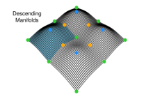
(a) Descending manifold

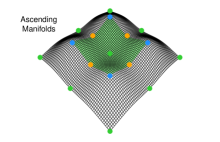
(b) Ascending manifold

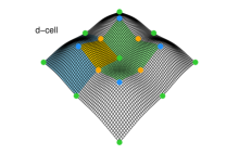
(c) $d$-cell

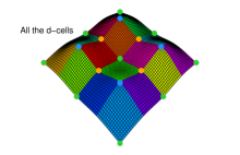
(d) Morse-Smale complex

Figure 1: An example of a Morse-Smale complex. The green dots are local minima; the blue dots are local modes; the violet dots are saddle points. Panels (a) and (b) give examples of descending $d$-manifolds (blue region) and an ascending $0$-manifold (green region). Panel (c) shows the corresponding $d$-cell (yellow region). Panel (d) is shows all $d$-cells.

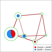
Figure 2: Graft-versus-Host Disease (GvHD) dataset (Brinkman et al., 2007). This is a $d=4$ dimensional dataset. We estimate the density difference based on the kernel density estimator and find regions where the two densities are significantly different. Then we visualize the density difference using the Morse-Smale complex. Each green circle denotes a $d$-cell, which is a partition for the support $\mathbb{K}$. The size of circle is proportional to the size of cell. If two cells are neighborhors, we add a line connecting them; the thickness of the line denotes the amount of boundary they share. The pie charts show the ratio of the regions within each cell where the two densities are significantly different from each other. See Section 3.4 for more details.

For all these applications, the Morse-Smale complex needs to be estimated. To the best of our knowledge, no theory has been developed for this estimation problem, prior to this paper. We have three goals in this paper: to show that many existing problems can be cast in terms of the Morse-Smale complex, to develop some new statistical methods based on the Morse-Smale complex, and to develop the statistical theory for estimating the complex.

Main results. The main results of this paper are:

1. Consistency of the Morse-Smale Complex. We prove the stability of the Morse-Smale complex (Theorem 28) in the following sense: if $B$ and $\widetilde{B}$ are boundaries of the descending $d$-manifolds (or ascending $0$-manifolds) of $p$ and $\widetilde{p}$ (defined in Section 2), then

   $${\sf Haus}(B,\widetilde{B})=O\left(\|\nabla p-\nabla\widetilde{p}\|_{\infty}\right).$$

2. Risk Bound for Mode clustering (mean-shift clustering; section 3.1): We bound the risk of mode clustering in Theorem 2.

3. Morse-Smale regression (section 3.2): In Theorems 4 and 38, we bound the risk of Morse-Smale regression, a multivariate regression method proposed in Gerber et al. (2010); Gerber and Potter (2011); Gerber et al. (2013) that synthesizes nonparametric regression and linear regression.

4. Morse-Smale signatures (section 3.3): We introduce a new visualization method for densities and regression functions.

5. Morse-Smale two-sample testing (section 3.4): We develop a new method for multivariate two-sample testing that can have good power.

Related work. The mathematical foundations for the Morse-Smale complex are from Morse theory (Morse, 1925, 1930; Milnor, 1963). Morse theory has many applications including computer vision (Paris and Durand, 2007), computational geometry (Cohen-Steiner et al., 2007) and topological data analysis (Chazal et al., 2014).

Previous work on the stability of the Morse-Smale complex can be found in Chen et al. (2016) and Chazal et al. (2014) but they only consider critical points rather than the whole Morse-Smale complex. Arias-Castro et al. (2016) prove pointwise convergence for the gradient ascent curves but this is not sufficient for proving the stability of the complex because the convergence of complexes requires convergence of multiple curves and the constants in the convergence rate derived from Arias-Castro et al. (2016) vary from points to points and some constants diverge when we are getting closer to the boundaries of complexes. Thus, we cannot obtain a uniform convergence of gradient ascent curves directly based on their results. Morse-Smale regression and visualization were proposed in Gerber et al. (2010); Gerber and Potter (2011); Gerber et al. (2013).

The R code (Algorithm 1, 2, and 3) used in this paper can be found at https://github.com/yenchic/Morse_Smale.

2 Morse Theory

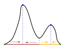
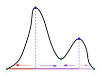
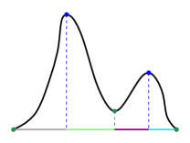
Figure 3: A one dimensional example. The blue dots are local modes and the green dots are local minima. Left panel: the basins of attraction for two local modes are colored by brown and orange. Middle panel: the basin of attraction (negative gradient) for the local minima are colored by red, purple and violet. Right panel: The intersection of the basins, which are called $d$-cells.

To motivate formal definitions, we start with the simple, one-dimensional example depicted in Figure 3. The left panel shows the sets associated with each local maximum (i.e. the basins of attraction of the maxima). The middle panel shows the sets associated with each local minimum. The right panel show the intersections of these basins, which gives the Morse-Smale complex defined by the function. Each interval in the complex, called a cell, is a region where the function is increasing or decreasing.

Now we give a formal definition. Let $f:\mathbb{K}\subset\mathbb{R}^{d}\mapsto\mathbb{R}$ be a function with bounded third derivatives that is defined on a compact set $\mathbb{K}$. Let $g(x)=\nabla f(x)$ and $H(x)=\nabla\nabla f(x)$ be the gradient and Hessian matrix of $f$, respectively, and let $\lambda_{j}(x)$ be the $j$th largest eigenvalue of $H(x)$. Define ${\cal C}=\{x\in\mathbb{K}:g(x)=0\}$ to be the set of all $f$’s critical points, which we call the critical set. Using the signs of the eigenvalues of the Hessian, the critical set ${\cal C}$ can be partitioned into $d+1$ distinct subsets $C_{0},\cdots,C_{d}$, where

$$C_{k}=\{x\in\mathbb{K}:g(x)=0,\lambda_{k}(x)>0,\lambda_{k+1}(x)<0\},\quad k=1,\cdots,d-1.$$ (1)

We define $C_{0},C_{d}$ to be the sets of all local maxima and minima (corresponding to all eigenvalues being negative and positive respectively). The set $C_{k}$ is called $k-$th order critical set.

A smooth function $f$ is called a Morse function (Morse, 1925; Milnor, 1963) if its Hessian matrix is non-degenerate at each critical point. That is, $|\lambda_{j}(x)|>0,\forall x\in{\cal C}$ for all $j$. In what follows we assume $f$ is a Morse function (actually, later we will assume further that $f$ is a Morse-Smale function).

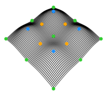
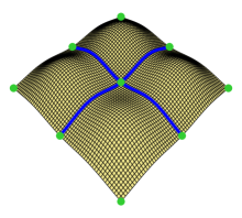
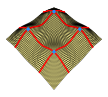
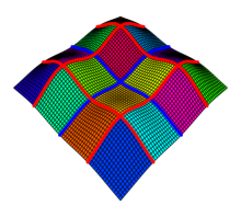
Figure 4: Two-dimensional examples of critical points, descending manifolds, ascending manifolds, and $2$-cells. This is the same function as Figure 1. (a): The set $C_{k}$ for $k=0,1,2$. The four blue dots are $C_{0}$, the collection of local modes (each of them is $c_{0,j}$ some $j=1,\cdots,4$). The four orange dots are $C_{1}$, the collection of saddle points (each of them is $c_{1,j}$ for some $j=1,\cdots,4$). The green dots are $C_{2}$, the collection of local minima (each green dot is $c_{2,j}$ for some $j=1,\cdots,9$). (b): The set $D_{k}$ for $k=0,1,2$. The yellow area is $D_{2}$ (each subregion separated by blue curves are $D_{2,j},j=1,\cdots,4$). The two blue curves are $D_{1}$ (each of the 4 blue segments are $D_{1,j},j=1,\cdots,4$). The green dots are $D_{0}$ (also $C_{2}$), the collection of local minima (each green dot is $D_{0,j}$ for some $j=1,\cdots,9$). (b): The set $A_{k}$ for $k=0,1,2$. The yellow area is $A_{0}$ (each subregion separated by red curves are $A_{0,j},j=1,\cdots,9$). The two red curves are $A_{1}$ (each of the 4 red segments are $A_{1,j},j=1,\cdots,4$). The blue dots are $A_{2}$ (also $C_{0}$), the collection of local modes (each green dot is $A_{0,j}$ for some $j=1,\cdots,4$). (d): Example for $2$-cells. The thick blue curves are $D_{1}$ and thick red curves are $A_{1}$.

Given any point $x\in\mathbb{K}$, we define the gradient ascent flow starting at $x$, $\pi_{x}:\mathbb{R}^{+}\mapsto\mathbb{K}$, by

$$\pi_{x}(0) =x$$ (2)

$$\pi^{\prime}_{x}(t) =g(\pi(t)).$$

A particle on this flow moves along the gradient from $x$ towards a “destination” given by

$$\operatorname{dest}(x)\equiv\lim_{t\rightarrow\infty}\pi_{x}(t).$$

It can be shown that $\operatorname{dest}(x)\in{\cal C}$ for $x\in\mathbb{K}$.

We can thus partition $\mathbb{K}$ based on the value of $\operatorname{dest}(x)$. These partitions are called descending manifolds in Morse theory (Morse, 1925; Milnor, 1963). Recall $C_{k}$ is the $k$-th order critical points, we assume $C_{k}=\{c_{k,1},\cdots,c_{k,m_{k}}\}$ contains $m_{k}$ distinct elements. For each $k$, define

$$D_{k} =\left\{x:\operatorname{dest}(x)\in C_{d-k}\right\}$$ (3)

$$D_{k,j} =\left\{x:\operatorname{dest}(x)=c_{d-k,j}\right\},\quad j=1,\cdots m_{d-k}.$$

That is, $D_{k}$ is the collection of all points whose gradient ascent flow converges to a $(d-k)$-th order critical point and $D_{k,j}$ is the collection of points whose gradient ascent flow converges to the $j$-th element of $C_{d-k}$. Thus, $D_{k}=\bigcup_{j=1}^{m_{d-k}}D_{k,j}$. From Theorem 4.2 in Banyaga and Hurtubise (2004), each $D_{k}$ is a disjoint union of $k$-dimensional manifolds ($D_{k,j}$ is a $k$-dimensional manifold). We call $D_{k,j}$ a descending k-manifold of $f$. Each descending k-manifold is a $k$-dimensional manifold such that the gradient flow from every point converges to the same $(d-k)$-th order critical point. Note that $\{D_{0},\cdots,D_{k}\}$ forms a partition of $\mathbb{K}$. The top panels of Figure 4 give an example of the descending manifolds for a two dimensional case.

The ascending manifolds are similar to descending manifolds but are defined through the gradient descent flow. More precisely, given any $x\in\mathbb{K}$, a gradient descent flow $\gamma:\mathbb{R}^{+}\mapsto\mathbb{K}$ starting from $x$ is given by

$$\gamma_{x}(0) =x$$ (4)

$$\gamma^{\prime}_{x}(t) =-g(\pi(t)).$$

Unlike the ascending flow defined in (2), $\gamma_{x}$ is a flow that moves along the gradient descent direction. The descent flow $\gamma_{x}$ shares similar properties to the ascent flow $\pi_{x}$; the limiting point $\lim_{t\rightarrow\infty}\gamma_{x}(t)\in{\cal C}$ is also in critical set when $f$ is a Morse function. Thus, similarly to $D_{k}$ and $D_{k,j}$, we define

$$A_{k} =\left\{x:\lim_{t\rightarrow\infty}\gamma_{x}(t)\in C_{d-k}\right\}$$ (5)

$$A_{k,j} =\left\{x:\lim_{t\rightarrow\infty}\gamma_{x}(t)=c_{d-k,j}\right\},\quad j=1,\cdots,m_{j-k}.$$

$A_{k}$ and $A_{k,j}$ have dimension $d-k$ and each $A_{k,j}$ is a partition for $A_{k}$ and $\{A_{0},\cdots,A_{d}\}$ consist of a partition for $\mathbb{K}$. We call each $A_{k,j}$ an ascending k-manifold to $f$.

A smooth function $f$ is called a Morse-Smale function if it is a Morse function and any pair of the ascending and descending manifolds of $f$ intersect each other transversely (which means that pairs of manifolds are not parallel at their intersections); see e.g. Banyaga and Hurtubise (2004) for more details. In this paper, we also assume that $f$ is a Morse-Smale function. Note that by the Kupka-Smale Theorem (see e.g. Theorem 6.6 in Banyaga and Hurtubise (2004)), Morse-Smale functions are generic (dense) in the collection of smooth functions. For more details, we refer to Section 6.1 in Banyaga and Hurtubise (2004).

A k-cell (also called Morse-Smale cell or crystal) is the non-empty intersection between any descending $k_{1}$-manifold and an ascending $(d-k_{2})$-manifold such that $k=\min\{k_{1},k_{2}\}$ (the ascending $(d-k_{2})$-manifold has dimension $k_{2}$). When we simply say a cell, we are referring to the $d$-cell since $d$-cells consists of the majority of $\mathbb{K}$ (the totality of $k$-cells with $k<d$ has Lebesgue measure 0). The Morse-Smale complex for $f$ is the collection of all $k$-cells for $k=0,\cdots,d$. The bottom panels of Figure 4 give examples for the ascending manifolds and the $d$-cells for $d=2$. Another example is given in Figure 1.

The cells of a smooth function can be used to construct an additive decomposition that is useful in data analysis. For a Morse-Smale function $f$, let $E_{1},\cdots,E_{L}$ be its associated cells. Then we can decompose $f$ into

$$f(x)=\sum_{\ell=1}^{L}f_{\ell}(x)1(x\in E_{\ell}),$$ (6)

where each $f_{\ell}(x)$ behaves like a multivariate isotonic function (Barlow et al., 1972; Bacchetti, 1989). Namely, $f(x)=f_{\ell}(x)$ when $x\in E_{\ell}$. This decomposition is because within each $E_{\ell}$, $f$ has exact a local mode and a local minimum on the boundary of $E_{\ell}$. The fact that $f$ admits such a decomposition will be used frequently in Section 3.2 and 3.3.

Among all descending/ascending manifolds, the descending $d$-manifolds and the ascending $0$-manifolds are often of great interest. For instance, mode clustering (Li et al., 2007; Azzalini and Torelli, 2007) uses the descending $d$-manifolds to partition the domain $\mathbb{K}$ into clusters. Morse-Smale regression (Gerber and Potter, 2011; Gerber et al., 2013) fits a linear regression individually over each $d$-cell (non-empty intersection of pairs of descending $d$-manifolds and ascending $0$-manifolds). Regions outside descending $d$-manifolds or ascending $0$-manifolds have Lebesgue measure $0$. Thus, later in our theoretical analysis, we will focus on the stability of the set $D_{d}$ and $A_{0}$ (see Section 4.1). We define boundaries of $D_{d}$ as

$$B\equiv\partial D_{d}=D_{d-1}\cup\cdots\cup D_{0}.$$ (7)

The set $B$ will be used frequently in Section 4.

3 Applications in Statistics

3.1 Mode Clustering

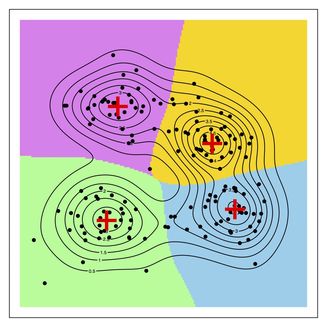
(a) Basins of attraction

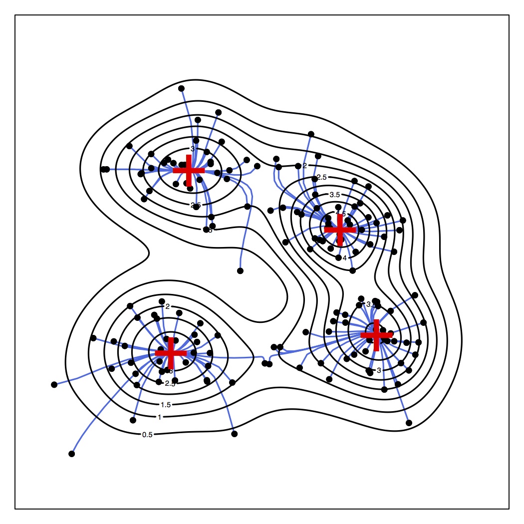
(b) Gradient ascent

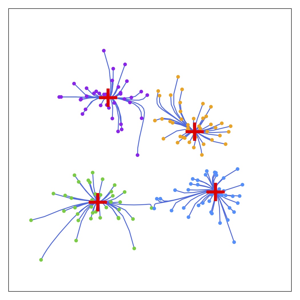
(c) Mode clustering

Figure 5: An example of mode clustering. (a): Basin of attraction for each local mode (red $+$). Black dots are data points. (b): Gradient flow (blue lines) for each data point. The gradient flow starts at one data point and ends at one local modes. (c): Mode clustering; we use the destination for gradient flow to cluster data points.

Mode clustering (Li et al., 2007; Azzalini and Torelli, 2007; Chacón and Duong, 2013; Arias-Castro et al., 2016; Chacón et al., 2015; Chen et al., 2016) is a clustering technique based on the Morse-Smale complex and is also known as mean-shift clustering (Fukunaga and Hostetler, 1975; Cheng, 1995; Comaniciu and Meer, 2002). Mode clustering uses the descending $d$-manifolds of the density function $p$ to partition the whole space $\mathbb{K}$. (Although the $d$-manifolds do not contain all points in $\mathbb{K}$, the regions outside $d$-manifolds have Lebesgue measure $0$). See Figure 5 for an example.

Now, we briefly describe the procedure of mode clustering. Let ${\cal X}=\{X_{1},\cdots,X_{n}\}$ be a random sample from density $p$ defined on a compact set $\mathbb{K}$ and assumed to be a Morse function. Recall that $\operatorname{dest}(x)$ is the destination of the gradient ascent flow starting from $x$. Mode clustering partitions the sample based on $\operatorname{dest}(x)$ for each point; specifically, it partitions ${\cal X}={\cal X}_{1}\bigcup\cdots\bigcup{\cal X}_{K}$ such that

$${\cal X}_{\ell}=\{X_{i}\in{\cal X}:\operatorname{dest}(X_{i})=m_{\ell}\},$$

where each $m_{\ell}$ is a local mode of $p$. We can also view mode clustering as a clustering technique based on the $d$-descending manifolds. Let $D_{d}=D_{d,1}\bigcup\cdots\bigcup D_{d,L}$ be the $d$-descending manifolds of $p$, assuming that $L$ is the number of local modes. Then each cluster ${\cal X}_{\ell}={\cal X}\bigcap D_{d,\ell}$.

In practice, however, we do not know $p$ so we have to use a density estimator $\widehat{p}_{n}$. A common density estimator is the kernel density estimator (KDE):

$$\widehat{p}_{n}(x)=\frac{1}{nh^{d}}\sum_{i=1}^{n}K\left(\frac{x-X_{i}}{h}\right),$$ (8)

where $K$ is a smooth kernel function and $h>0$ is the smoothing parameter. Note that mode clustering is not limited to the KDE; other density estimators also give us a sample-based mode clustering. Based on the KDE, we are able to estimate gradient $\widehat{g}_{n}(x)$, the gradient flows $\widehat{\pi}_{x}(t)$, and the destination $\widehat{\operatorname{dest}}_{n}(x)$ (note that the mean shift algorithm is an algorithm to perform these tasks). Thus, we can estimate the $d$-descending manifolds by the plug-in from $\widehat{p}_{n}$. Let $\widehat{D}_{d}=\widehat{D}_{d,1}\bigcup\cdots\bigcup\widehat{D}_{d,\widehat{L}}$ be the $d$-descending manifolds of $\widehat{p}_{n}$, where $\widehat{L}$ is the number of local modes of $\widehat{p}_{n}$. The estimated clusters will be $\widehat{{\cal X}}_{1},\cdots,\widehat{{\cal X}}_{\widehat{L}}$, where each $\widehat{{\cal X}}_{\ell}={\cal X}\bigcap\widehat{D}_{d,\ell}$. Figure 5 displays an example of mode clustering using the KDE.

A nice property of mode clustering is that there is a clear population quantity that our estimator (clusters based on the given sample) is estimating: the population partition of the data points. Thus we can consider properties of the procedure such as consistency, which we discuss in detail in Section 4.2.

3.2 Morse-Smale Regression

Let $(X,Y)$ be a random pair where $Y\in\mathbb{R}$ and $X_{i}\in\mathbb{K}\subset\mathbb{R}^{d}$. Estimating the regression function $m(x)=\mathbb{E}[Y|X=x]$ is challenging for $d$ of even moderate size. A common way to address this problem is to use a simple regression function that can be estimated with low variance. For example, one might use an additive regression of the form $m(x)=\sum_{j}m_{j}(x_{j})$ which is a sum of one-dimensional smooth functions. Although the true regression function is unlikely to be of this form, it is often the case that the resulting estimator is useful.

A different approach, Morse-Smale regression (MSR), is suggested in Gerber et al. (2013). This takes advantage of the (relatively) simple structure of the Morse-Smale complex and the isotone behavior of the function on each cell. Specifically, MSR constructs a piecewise linear approximation to $m(x)$ over the cells of the Morse-Smale complex.

We first define the population version of the MSR. Let $m(x)=\mathbb{E}(Y|X=x)$ be the regression function and is assumed to be a Morse-Smale function. Let $E_{1},\cdots E_{L}$ be the $d$-cells for $m$. The Morse-Smale Regression for $m$ is a piecewise linear function within each cell $E_{\ell}$ such that

$$m_{{\sf MSR}}(x)=\mu_{\ell}+\beta_{\ell}^{T}x,\mbox{ for }x\in E_{\ell},$$ (9)

where $(\mu_{\ell},\beta_{\ell})$ are obtained by minimizing mean square error:

$$(\mu_{\ell},\beta_{\ell}) =\underset{\mu,\beta}{\sf\mathop{\mathrm{argmin}}}\,\,\mbox{ }\mathbb{E}\left((Y-m_{{\sf MSR}}(X))^{2}|X\in E_{\ell}\right)$$ (10)

$$=\underset{\mu,\beta}{\sf\mathop{\mathrm{argmin}}}\,\,\mbox{ }\mathbb{E}\left((Y-\mu-\beta^{T}X)^{2}|X\in E_{\ell}\right)$$

That is, $m_{{\sf MSR}}$ is the best linear piecewise predictor using the $d$-cells. One can also view MSR as using a linear function to approximate $f_{\ell}$ in the additive model (6). Note that $m_{{\sf MSR}}$ is well defined except on the boundaries of $E_{\ell}$ that have Lebesgue measure $0$.

Now we define the sample version of the MSR. Let $(X_{1},Y_{1}),\cdots,(X_{n},Y_{n})$ be the random sample from the probability measure $\mathbb{P}_{X}\times\mathbb{P}_{Y}$ such that $X_{i}\in\mathbb{K}\subset\mathbb{R}^{d}$ and $Y_{i}\in\mathbb{R}$. Throughout section 3.2, we assume the density of covariates $X$ is bounded, positive and has a compact support $\mathbb{K}$ and the response $Y$ has finite second moment.

Let $\widehat{m}_{n}$ be a smooth nonparametric regression estimator for $m$. We call $\widehat{m}_{n}$ the pilot estimator. For instance, one may use the kernel regression Nadaraya (1964) $\widehat{m}_{n}(x)=\frac{\sum_{i=1}^{n}Y_{i}K\left(\frac{x-X_{i}}{h}\right)}{\sum_{i=1}^{n}K\left(\frac{x-X_{i}}{h}\right)}$ as the pilot estimator. We define $d$-cells for $\widehat{m}_{n}$ as $\widehat{E}_{1},\cdots,\widehat{E}_{\widehat{L}}$. Using the data $(X_{i},Y_{i})$ within each estimated $d$-cell, $\widehat{E}_{\ell}$, the MSR for $\widehat{m}_{n}$ is given by

$$\widehat{m}_{n,{\sf MSR}}(x)=\widehat{\mu}_{\ell}+\widehat{\beta}_{\ell}^{T}x,\mbox{ for }x\in\widehat{E}_{\ell},$$ (11)

where $(\widehat{\mu}_{\ell},\widehat{\beta}_{\ell})$ are obtained by minimizing the empirical squared error:

$$(\widehat{\mu}_{\ell},\widehat{\beta}_{\ell})=\underset{\mu,\beta}{\sf\mathop{\mathrm{argmin}}}\mbox{ }\sum_{i:X_{i}\in\widehat{E}_{\ell}}(Y_{i}-\mu-\beta^{T}X_{i})^{2}$$ (12)

This MSR is slightly different from the original version in Gerber et al. (2013). We will discuss the difference in Remark 1. Computing the parameters of MSR is not very difficult–we only need to compute the cell labels of each observation (this can be done by the mean shift algorithm or some fast variants such as the quick-shift algorithm Vedaldi and Soatto 2008) and then fit a linear regression within each cell.

MSR may give low prediction error in some cases; see Gerber et al. (2013) for some concrete examples. In Theorem 38, we prove that we may estimate $m_{{\sf MSR}}$ at a fast rate. Moreover, the regression function may be visualized by the methods discussed later.

Remark 1

The original version of Morse-Smale regression proposed in Gerber et al. (2013) does not use $d$-cells of a pilot nonparametric estimate $\widehat{m}_{n}$. Instead, they directly find local modes and minima using the original data points $(X_{i},Y_{i})$. This saves computational effort but comes with a price: there is no clear population quantity being estimated by their approach. That is, when the sample size increases to infinity, there is no guarantee that their method will converge. In our case, we apply a consistent pilot estimate for $m$ and construct $d$-cells on this pilot estimate. As is shown in Theorem 4, our method is consistent for this population quantity.

3.3 Morse-Smale Signatures and Visualization

In this section we define a new method for visualizing multivariate functions based on the Morse-Smale complex, called Morse-Smale signatures. The idea is very similar to the Morse-Smale regression but the signatures can be applied to any Morse-Smale function.

Let $E_{1},\cdots,E_{K}$ be the $d$-cells (nonempty intersection of a descending $d$-manifold and an ascending $0$-manifold) for a Morse-Smale function $f$ that has a compact support $\mathbb{K}$. The function $f$ depends on the context of the problem. For density estimation, $f$ is the density $p$ or its estimator $\widehat{p}_{n}$. For regression problem, $f$ is the regression function $m$ or a nonparametric estimator $\widehat{m}_{n}$ . For two sample test, $f$ is the density difference $p_{1}-p_{2}$ or the estimated density difference $\widehat{p}_{1}-\widehat{p}_{2}$. Note that $E_{1},\cdots,E_{K}$ form a partition for $\mathbb{K}$ except a Lebesgue measure $0$ set. Each cell corresponds to a unique pair of a local mode and a local minimum. Thus, the local modes and minima along with $d$-cells form a bipartite graph which we call it signature graph. The signature graph contains geometric information about $f$. See Figure 6 and 7 for examples.

The signature is defined as follows. We project the maxima and minima of the function into $\mathbb{R}^{2}$ using multidimensional scaling. We connect a maximum and minimum by an edge if there exists a cell that connects them. The width of the edge is proportional to the norm of the linear coefficients of the linear approximation to the function within the cell. The linear approximation is

$$f_{{\sf MS}}(x)=\eta^{\dagger}_{\ell}+\gamma^{\dagger T}_{\ell}x,\quad\mbox{for }x\in E_{\ell},$$ (13)

where $\eta_{\ell}^{\dagger}\in\mathbb{R}$ and $\gamma_{\ell}^{\dagger}\in\mathbb{R}^{d}$ are parameters from

$$(\eta_{\ell}^{\dagger},\gamma_{\ell}^{\dagger})=\underset{\eta,\gamma}{\sf argmin}\int_{E_{\ell}}\left(f(x)-\eta-\gamma^{T}x\right)^{2}dx.$$ (14)

This is again a linear approximation for $f_{\ell}$ in the additive model (6). Note that $f_{{\sf MS}}$ may not be continuos when we move from one cell to another. The summary statistics for the edge associated with cell $E_{\ell}$ are the parameters $(\eta_{\ell}^{\dagger},\gamma_{\ell}^{\dagger})$. We call the function $f_{{\sf MS}}$ the (Morse-Smale) approximation function; it is the best piecewise-linear representation for $f$ (piecewise linear within each cell) under ${\cal L}_{2}$ error given the $d$-cells. This function is well-defined except on a set of Lebesgue measure $0$ (the boundaries of each cell). See Figure 6 for a example on the approximation function. The details are in Algorithm 1.

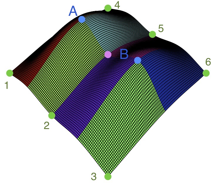
(a) Original function

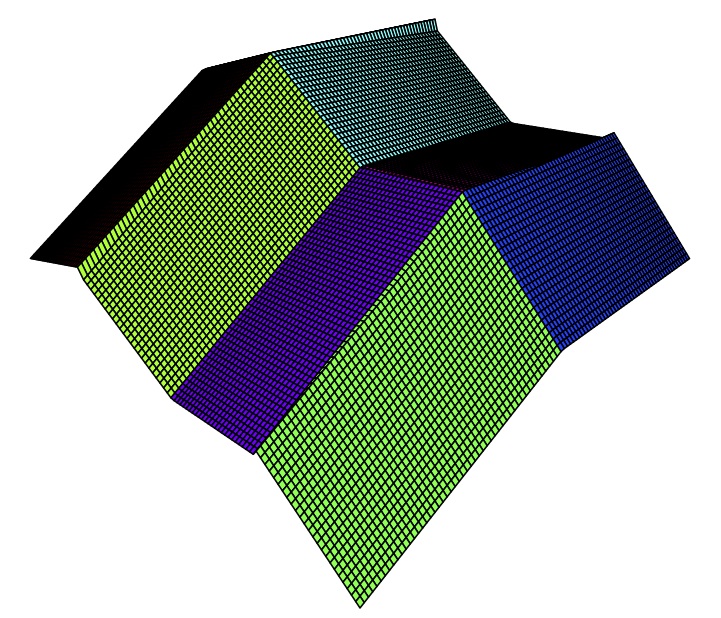
(b) Approximation function

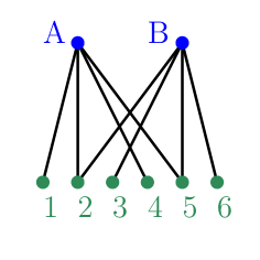
(c) Signature graph

Figure 6: Morse-Smale signatures for a smooth function. (a): The original function. The blue dots are local modes, the green dots are local minima and the pink dot is a saddle point. (b): The Morse-Smale approximation to (a). This is the best piecewise linear approximation to the original function given $d$-cells. (c): This bipartite graph has nodes that are local modes and minima and edges that represent the $d$-cells. Note that we can summarize the smooth function (a) by the signature graph (c) and the parameters for constructing approximation function (b). The signature graph and parameters for approximation function define the Morse-Smale signatures.

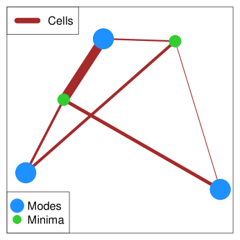
Figure 7: Morse-Smale Signature visualization (Algorithm 1) of the density difference for GvHD dataset (see Figure 2). The blue dots are local modes; the green dots are local minima; the brown lines are $d$-cells. These dots and lines form the signature graph. The width indicates the ${\cal L}_{2}$ norm for the slope of regression coefficients. i.e. $\|\gamma^{\dagger}_{\ell}\|$. The location for modes and minima are obtained by multidimensional scaling so that the relative distance is preserved.

Example. Figure 7 is an example using the GvHD dataset. We first conduct multidimensional scaling (Kruskal, 1964) on the local modes and minima for $f$ and plot them on the 2-D plane. In Figure 7, the blue dots are local modes and the green dots are local minima. These dots act as the nodes for the signature graph. Then we add edges, representing the cells for $f$ that connect pairs of local modes and minima, to form the signature graph. Lastly, we adjust the width for the edges according to the strength (${\cal L}_{2}$ norm) of regression function within each cell (i.e. $\|\gamma^{\dagger}_{\ell}\|$). Algorithm 1 provides a summary for visualizing a general multivariate function using what we described in this paragraph.

Algorithm 1 Visualization using Morse-Smale Signatures

Input: Grid points $x_{1},\cdots,x_{N}$ and the functional evaluations $f(x_{1}),\cdots,f(x_{N})$.

1. Find local modes and minima of $f$ on the discretized points $x_{1},\cdots,x_{N}$. Let $M_{1},\cdots M_{K}$ and $m_{1},\cdots,m_{S}$ denote the grid points for modes and minima.

2. Partition $\{x_{1},\cdots,x_{N}\}$ into $\mathcal{X}_{1},\cdots\mathcal{X}_{L}$ according to the $d$-cells of $f$ (1. and 2. can be done by using a k-nearest neighbor gradient ascent/descent method; see Algorithm 1 in Gerber et al. (2013)).

3. For each cell $\mathcal{X}_{\ell}$, fit a linear regression with $(X_{i},Y_{i})=(x_{i},f(x_{i}))$, where $x_{i}\in\mathcal{X}_{\ell}$. Let the regression coefficients (without intercept) be $\beta_{\ell}$.

4. Apply multidimensional scaling to modes and minima jointly. Denote their 2 dimensional representation points as

$$\{M^{*}_{1},\cdots M^{*}_{K},m^{*}_{1},\cdots,m^{*}_{S}\}.$$

5. Plot $\{M^{*}_{1},\cdots M^{*}_{K},m^{*}_{1},\cdots,m^{*}_{S}\}$.

6. Add edge to a pair of mode and minimum if there exist a cell that connects them. The width of the edge is in proportional to $\|\beta_{\ell}\|$ (for cell $\mathcal{X}_{\ell}$).

3.4 Two Sample Comparison

The Morse-Smale complex can be used to compare two samples. There are two ways to do this. The first one is to test the difference in two density functions locally and then use the Morse-Smale signatures to visualize regions where the two samples are different. The second approach is to conduct a nonparametric two sample test within each Morse-Smale cell. The advantage of the first approach is that we obtain a visual display on where the two densities are different. The merit of the second method is that we gain additional power in testing the density difference by using the shape information.

3.4.1 Visualizing the Density Difference

Let $X_{1},\ldots X_{n}$ and $Y_{1},\ldots,Y_{m}$ be two random sample with densities $p_{X}$ and $p_{Y}$. In a two sample comparison, we not only want to know if $p_{X}=p_{Y}$ but we also want to find the regions that they significantly disagree. That is, we are doing the local tests

$$H_{0}(x):p_{X}(x)=p_{Y}(x)$$ (15)

simultaneously for all $x\in\mathbb{K}$ and we are interested in the regions where we reject $H_{0}(x)$. A common approach is to estimate the density for both sample by the KDE and set a threshold to pickup those regions that the density difference is large. Namely, we first construct density estimates

$$\widehat{p}_{X}(x)=\frac{1}{nh^{d}}\sum_{i=1}^{n}K\left(\frac{x-X_{i}}{h}\right),\quad\widehat{p}_{Y}(x)=\frac{1}{mh^{d}}\sum_{i=1}^{m}K\left(\frac{x-Y_{i}}{h}\right)$$ (16)

and then compute $\widehat{f}(x)=\widehat{p}_{X}(x)-\widehat{p}_{Y}(x)$. The regions

$$\Gamma(\lambda)=\left\{x\in\mathbb{K}:|\widehat{f}(x)|>\lambda\right\}$$ (17)

are where we have strong evidence to reject $H_{0}(x)$. The threshold $\lambda$ can be picked by quantile values of the bootstrapped ${\cal L}_{\infty}$ density deviation to control type 1 error or can be chosen by controlling the false discovery rate (Duong, 2013).

Unfortunately, $\Gamma(\lambda)$ is hard to visualize when $d>3$. So we use the Morse-Smale complex for $\widehat{f}$ and visualize $\Gamma(\lambda)$ by its behavior on the $d$-cells of the complex. Algorithm 2 gives a method for visualizing density differences like $\Gamma(\lambda)$ in the context of comparing two independent samples.

Algorithm 2 Visualization For Two Sample Test

Input: Sample 1: $\{X_{1},...X_{n}\}$, Sample 2: $\{Y_{1},\cdots,Y_{m}\}$, threshold $\lambda$ and radius constant $r_{0}$

1. Compute the density estimates $\widehat{p}_{X}$ and $\widehat{p}_{Y}$.

2. Compute the difference function $\widehat{f}=\widehat{p}_{X}-\widehat{p}_{Y}$ and the significant regions

$$\Gamma^{+}(\lambda)=\left\{x\in\mathbb{K}:\widehat{f}(x)>\lambda\right\},\quad\Gamma^{-}(\lambda)=\left\{x\in\mathbb{K}:\widehat{f}(x)<-\lambda\right\}$$ (18)

3. Find the $d$-cells for $\widehat{f}$, denoted as $E_{1},\cdots,E_{L}$.

4. For cell $E_{\ell}$, do (4-1) and (4-2):

4-1. compute the cell center $e_{\ell}$, cell size $V_{\ell}={\sf Vol}(E_{\ell})$,

4-2. compute the positive significant ratio and negative significant ratio

$$r^{+}_{\ell}=\frac{{\sf Vol}(E_{\ell}\cap\Gamma^{+}(\lambda))}{{\sf Vol}(E_{\ell})},\quad r^{-}_{\ell}=\frac{{\sf Vol}(E_{\ell}\cap\Gamma^{-}(\lambda))}{{\sf Vol}(E_{\ell})}.$$ (19)

5. For every pair of cell $E_{j}$ and $E_{\ell}$ $(j\neq\ell)$, compute the shared boundary size:

$$B_{j\ell}={\sf Vol}_{d-1}(\bar{E}_{j}\cap\bar{E}_{\ell}),$$ (20)

where ${\sf Vol}_{d-1}$ is the $d-1$ dimensional Lebesgue measure.

6. Do multidimensional scaling (Kruskal, 1964) to $e_{1},\cdots,e_{L}$ to obtain low dimensional representation $\widetilde{e}_{1},\cdots,\widetilde{e}_{L}$.

7. Place a ball center at each $\widetilde{e}_{\ell}$ with radius $r_{0}\times\sqrt{V_{\ell}}$.

8. If $r^{+}_{\ell}+r^{-}_{\ell}>0$, add a pie chart center at $\widetilde{e}_{\ell}$ with radius $r_{0}\times\sqrt{V_{\ell}}\times(r^{+}_{\ell}+r^{-}_{\ell})$. The pie chart contains two groups, each with ratio $\left(\frac{r^{+}_{\ell}}{r^{+}_{\ell}+r^{-}_{\ell}},\frac{r^{-}_{\ell}}{r^{+}_{\ell}+r^{-}_{\ell}}\right)$.

9. Add a line to connect two nodes $\widetilde{e}_{j}$ and $\widetilde{e}_{\ell}$ if $B_{j\ell}>0$. We may adjust the thickness of the line according to $B_{j\ell}$.

An example for Algorithm 2 is in Figure 2, in which we apply the visualization algorithm for the the GvHD dataset by using kernel density estimator. We choose the threshold $\lambda$ by bootstrapping the ${\cal L}_{\infty}$ difference for $\widehat{f}$ i.e. $\sup_{x}|\widehat{f}^{*}(x)-\widehat{f}(x)|$, where $\widehat{f}^{*}$ is the density difference for the bootstrap sample. We pick $\alpha=95\%$ upper quantile value for the bootstrap deviation as the threshold.

The radius constant $r_{0}$ is defined by the user. It is a constant for visualization and does not affect the analysis. Algorithm 2 preserves the relative position for each cell and visualizes the cell according to its size. The pie-chart provides the ratio of regions where the two densities are significantly different. The lines connecting two cells provide the geometric information about how cells are connected to each other.

By applying Algorithm 2 to the GvHD dataset (Figure 2), we find that there are 6 cells and one cell much larger than the others. Moreover, in most regions, the blue regions are larger than the red areas. This indicates that compared to the density of the control group, the density of the GvHD group seem to concentrates more so that the regions above the threshold are larger.

3.4.2 Morse-Smale Two-Sample Test

Here we introduce a technique combining the energy test (Baringhaus and Franz, 2004; Székely and Rizzo, 2004, 2013) and the Morse-Smale complex to conduct a two sample test. We call our method the Morse-Smale Energy test (MSE test). The advantage of the MSE test is that it is a nonparametric test and its power can be higher than the energy test; see Figure 8. Moreover, we can combine our test with the visualization tool proposed in the previous section (Algorithm 2); see Figure 9 for an example for displaying p-values from MSE test when visualizing the density difference.

Before we introduce our method, we first review the ordinary energy test. Given two random variables $X\in\mathbb{R}^{d}$ and $Y\in\mathbb{R}^{d}$, the energy distance is defined as

$${\cal E}(X,Y)=2\mathbb{E}\|X-Y\|-\mathbb{E}\|X-X^{\prime}\|-\mathbb{E}\|Y-Y^{\prime}\|,$$ (21)

where $X^{\prime}$ and $Y^{\prime}$ are iid copies of $X$ and $Y$. The energy distance has several useful applications such as the goodness-of-fit testing (Székely and Rizzo, 2005), two sample testing (Baringhaus and Franz, 2004; Székely and Rizzo, 2004, 2013), clustering (Szekely and Rizzo, 2005), and distance components (Rizzo et al., 2010) to name but few. We recommend an excellent review paper in (Székely and Rizzo, 2013).

For the two sample test, let $X_{1},\cdots,X_{n}$ and $Y_{1},\cdots,Y_{m}$ be the two samples we want to test. The sample version of energy distance is

$$\widehat{{\cal E}}(X,Y)=\frac{2}{nm}\sum_{i=1}^{n}\sum_{j=1}^{m}\|X_{i}-Y_{j}\|-\frac{1}{n^{2}}\sum_{i=1}^{n}\sum_{j=1}^{n}\|X_{i}-X_{j}\|-\frac{1}{m^{2}}\sum_{i=1}^{m}\sum_{j=1}^{m}\|Y_{i}-Y_{j}\|.$$ (22)

If $X$ and $Y$ are from the sample population (the same density), $\widehat{{\cal E}}(X,Y)\overset{P}{\rightarrow}0$. Numerically, we use the permutation test for computing the p-value for $\widehat{{\cal E}}(X,Y)$. This can be done quickly in the R-package ‘energy’ (Rizzo and Szekely, 2008).

Now we formally introduce our testing procedure: the MSE test (see Algorithm 3 for a summary). Our test consists of three steps. First, we split the data into two halves. Second, we use one half of the data (contains both samples) to do a nonparametric density estimation (e.g. the KDE) and then compute the Morse-Smale complex ($d$-cells). Last, we use the other half of the data to conduct the energy distance two sample test ‘within each $d$-cell’. That is, we partition the second half of the data by the $d$-cells. Within each cell, we do the energy distance test. If we have $L$ cells, we will have $L$ p-values from the energy distance test. We reject $H_{0}$ if any one of the $L$ p-values is smaller than $\alpha/L$ (this is from Bonferroni correction). Figure 9 provides an example for using the above procedure (Algorithm 3) along with the visualization method proposed in Algorithm 2. Data splitting is used to avoid using the same data twice, which ensures we have a valid test.

Algorithm 3 Morse-Smale Energy Test (MSE test)

Input: Sample 1: $\{X_{1},...X_{n}\}$, Sample 2: $\{Y_{1},\cdots,Y_{m}\}$, smoothing parameter $h$, significance level $\alpha$

1. Randomly split the data into halves ${\cal D}_{1}$ and ${\cal D}_{2}$; both contain equal number of $X$ and $Y$ (assuming $n$ and $m$ are even).

2. Compute the KDE $\widehat{p}_{X}$ and $\widehat{p}_{Y}$ by the first sample ${\cal D}_{1}$.

3. Find the $d$-cells for $\widehat{f}=\widehat{p}_{X}-\widehat{p}_{Y}$, denoted as $E_{1},\cdots,E_{L}$.

4. For cell $E_{\ell}$, do 4-1 and 4-2:

4-1. Find $X$ and $Y$ in the second sample ${\cal D}_{2}$,

4-2. Do the energy test for two sample comparison. Let the p-value be $p(\ell)$

5. Reject $H_{0}$ if $p(\ell)<\alpha/L$ for some $\ell$.

Example. Figure 8 shows a simple comparison for the proposed MSE test to the usual Energy test. We consider a $K=4$ Gaussian mixture model in $d=2$ with standard deviation of each component being the same $\sigma=0.2$ and the proportion for each component is $(0.2,0.5,0.2,0.1)$. The left panel displays a sample with $N=500$ from this mixture distribution. We draw the first sample from this Gaussian mixture model. For the second sample, we draw a similar Gaussian mixture model except that we change the deviation of one component. In the middle panel, we change the deviation to the third component (C3 in left panel, which contains $20\%$ data points). In the right panel, we change the deviation to the fourth component (C4 in left panel, which contains $10\%$ data points). We use significance level $\alpha=0.05$ and for MSE test, we consider the Bonferroni correction and the smoothing bandwidth is chosen using Silverman’s rule of thumb (Silverman, 1986).

Note that in both the middle and the right panels, the left most case (added deviation equals $0$) is where $H_{0}$ should not be rejected. As can be seen from Figure 8, the MSE test has much stronger power compared to the usual Energy test.

The original energy test has low power while the MSE test has higher power. This is because the two distributions only differ at a small portion of the regions so that a global test like energy test requires large sample sizes to detect the difference. On the other hand, the MSE test partitions the space according to the density difference so that it is capable of detecting the local difference.

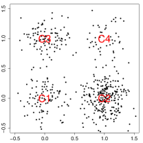
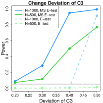
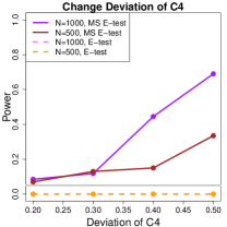
Figure 8: An example comparing the Morse-Smale Energy test to the original Energy test. We consider a $d=2$, $K=4$ Gaussian mixture model. Left panel: an instance for the Gaussian mixture. We have four mixture components, denoting as C1, C2, C3 and C4. They have equal standard deviation ($\sigma=0.2$) and the proportions for each components are $(0.2,0.5,0.2,0.1)$. Middle panel: We changed the standard deviations of component C3 to $0.3,0.4$ and $0.5$ and compute the power for the MSE test and the usual Energy test at sample size $N=500$ and $1000$. (Standard deviation equals $0.2$ is where $H_{0}$ should not be rejected.) Right panel: We add the variance of component C4 (the smallest component) and do the same comparison as in the middle panel. We pick the significance level $\alpha=0.05$ (gray horizontal line) and in the MSE test, we reject $H_{0}$ if the minimal p-value is less than $\alpha/L$, where $L$ is the number of cells (i.e. we are using the Bonferroni correction).

Example. In addition to the higher power, we may combine the MSE test with the visualization tool in Algorithm 2. Figure 9 displays an example where we visualize the density difference and simultaneously indicate the p-values from the Energy test within each cell using the GvHD dataset. This provides us more information about how two distributions differ from each other.

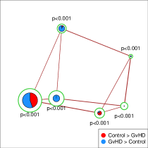
Figure 9: An example using both Algorithm 2 and 3 to the GvHD dataset introduced in Figure 2. We use data splitting as described in Algorithm 3. For the first part of the data, we compute the cells and visualize the cells using Algorithm 2. Then we apply the energy distance two sample test for each cell as described in Algorithm 3 and we annotate each cell with a p-value. Note that the visualization is slightly different to Figure 2 since we use only half of the original dataset in this case.

4 Theoretical Analysis

We first define some notation for the theoretical analysis. Let $f$ be a smooth function. We define $\|f\|_{\infty}=\sup_{x}|f(x)|$ to be the ${\cal L}_{\infty}$-norm of $f$. In addition, let $\|f\|_{j,\max}$ denote the elementwise ${\cal L}_{\infty}$-norm for $j$-th derivatives of $f$. For instance,

$$\|f\|_{1,\max}=\max_{i}\|g_{i}(x)\|_{\infty},\quad\|f\|_{2,\max}=\max_{i,j}\|H_{ij}(x)\|_{\infty}.$$

We also define $\|f\|_{0,\max}=\|f\|_{\infty}$. We further define

$$\|f\|^{*}_{\ell,\max}=\max\left\{\|f\|_{j,\max}:j=0,\cdots,\ell\right\}.$$ (23)

The quantity $\|f-h\|^{*}_{\ell,\max}$ measures the difference between two functions $f$ and $h$ up to $\ell$-th order derivative.

For two sets $A,B$, the Hausdorff distance is

$${\sf Haus}(A,B)=\inf\{r:A\subset B\oplus r,B\subset A\oplus r\},$$ (24)

where $A\oplus r=\{y:\min_{x\in A}\|x-y\|\leq r\}$. The Hausdorff distance is like the ${\cal L}_{\infty}$ distance for sets.

Let $\widetilde{f}:\mathbb{K}\subset\mathbb{R}^{d}\mapsto\mathbb{R}$ be a smooth function with bounded third derivatives. Note that as long as $\|\widetilde{f}-f\|^{*}_{3,\max}$ is small, $\widetilde{f}$ is also a Morse function by Lemma 9. Let $\widetilde{D}$ denote the boundaries of the descending $d$-manifolds of $\widetilde{f}$. We will show if $\|f-\widetilde{f}\|^{*}_{3,\max}$is sufficiently small, then ${\sf Haus}(\widetilde{D},D)=O(\|\widetilde{f}-f\|_{1,\max})$.

4.1 Stability of the Morse-Smale Complex

Before we state our theorem, we first derive some properties of descending manifolds. Recall that we are interested in $B=\partial D_{d}$, the boundary of the descending $d$-manifolds (and $B$ is also the union of all $j$-descending manifolds for $j<d$). Since each $D_{j}$ is a collection of smooth $j$-dimensional manifolds embedded in $\mathbb{R}^{d}$, for every $x\in D_{j}$, there exists a basis $v_{1}(x),\cdots,v_{d-j}(x)$ such that each $v_{k}(x)$ is perpendicular to $D_{j}$ at $x$ for $k=1,\cdots d-j$ (Bredon, 1993; Helgason, 1979). That is, $v_{1}(x),\cdots,v_{d-j}(x)$ span the normal space to $D_{j}$ at $x$. For simplicity, we write

$$V(x)=(v_{1}(x),\cdots,v_{d-j}(x))\in\mathbb{R}^{d\times(d-j)}$$ (25)

for $x\in D_{j}$.

Note the number of columns $d-j\equiv d-j(x)$ in $V(x)$ depends on which $D_{j}$ the point $x$ belongs to. We use $j$ rather than $j(x)$ to simplify the notation. For instance, if $x\in D_{1}$, $V(x)\in\mathbb{R}^{d\times(d-1)}$ and if $x\in D_{d-1}$, $V(x)\in\mathbb{R}^{d\times 1}$. We also let

$$\mathbb{V}(x)={\rm span}\{v_{1}(x),\cdots,v_{d-j}(x)\}$$ (26)

denote the normal space to $B$ at $x$. One can view $\mathbb{V}(x)$ as the normal map of the manifold $D_{j}$ at $x\in D_{j}$.

For each $x\in B$, define the projected Hessian

$$H_{V}(x)=V(x)^{T}H(x)V(x),$$ (27)

which is the Hessian matrix of $p$ by taking gradients along column space of $V(x)$. If $x\in D_{j}$, $H_{V}(x)$ is a $(d-j)\times(d-j)$ matrix. The eigenvalues of $H_{V}(x)$ determine how the gradient flows are moving away from $B$. We let $\lambda_{\min}(M)$ be the smallest eigenvalue for a symmetric matrix $M$. If $M$ is a scalar (just one point), then $\lambda_{\min}(M)=M$.

Assumption (D): We assume that $H_{\min}=\min_{x\in B}\lambda_{\min}(H_{V}(x))>0.$

This assumption is very mild; it requires that the gradient flow moves away from the boundary of ascending manifolds. In terms of mode clustering, this requires the gradient flow to move away from the boundaries of clusters. For a point $x\in D_{d-1}$, let $v_{1}(x)$ be the corresponding normal direction. Then the gradient $g(x)$ is normal to $v_{1}(x)$ by definition. That is, $v_{1}(x)^{T}g(x)=v_{1}(x)^{T}\nabla p(x)=0$, which means that the gradient along $v_{1}(x)$ is $0$. Assumption (D) means that the the second derivative along $v_{1}(x)$ is positive, which implies that the density along direction $v_{1}(x)$ behaves like a local minimum at point $x$. Intuitively, this is how we expect the density to behave around the boundaries: gradient flows are moving away from the boundaries (except for those flows that are already on the boundaries).

Theorem 1 (Stability of descending $d$-manifolds)

Let $f,\widetilde{f}:\mathbb{K}\subset\mathbb{R}^{d}\mapsto\mathbb{R}$ be two smooth functions with bounded third derivatives defined as above and let $B,\widetilde{B}$ be the boundaries of the associated ascending manifolds. Assume $f$ is a Morse function satisfying condition (D). When $\|f-\widetilde{f}\|^{*}_{3,\max}$ is sufficiently small,

$${\sf Haus}(\widetilde{B},B)=O(\|\widetilde{f}-f\|_{1,\max}).$$ (28)

This theorem shows that the boundaries of descending $d$-manifolds for two Morse functions are close to each other and the difference between the boundaries is controlled by the rate of the first derivative difference.

Similarly to descending manifolds, we can define all the analogous quantities for ascending manifolds. We introduce the following assumption:

Assumption (A): We assume $H_{\max}=\max_{x\in\partial A_{0}}\lambda_{\max}(H_{V}(x))<0.$

Note that $\lambda_{\max}(M)$ denotes the largest eigenvalue of a matrix $M$. If $M$ is a scalar, $\lambda_{\max}(M)=M$. Under assumption (A), we have a similar stability result (Theorem 28) for ascending manifolds. Assumptions (A) and (D) together imply the stability of $d$-cells.

Theorem 28 can be applied to nonparametric density estimation. Our goal is to estimate the boundary of the descending $d$-manifolds, $B$, of the unknown population density function $p$. Our estimator is $\widehat{B}_{n}$, the boundary of the descending $d$-manifolds to a nonparametric density estimator e.g. the kernel density estimate $\widehat{p}_{n}$. Then under certain regularity condition, their difference is given by

$${\sf Haus}\left(\widehat{B}_{n},B\right)=O\left(\|\widehat{p}_{n}-p\|_{1,\max}\right).$$

We will see this result in the next section when we discuss mode clustering.

Similar reasoning works for the nonparametric regression case. Assume that we are interested in $B$, the boundary of descending $d$-manifolds, for the regression function $m(x)=\mathbb{E}(Y|X=x)$. And our estimator $\widehat{B}$ is again a plug-in estimate based on $\widehat{m}_{n}(x)$, a nonparametric regression estimator (e.g., kernel estimator). Then under mild regularity conditions,

$${\sf Haus}\left(\widehat{B}_{n},B\right)=O\left(\|\widehat{m}_{n}-m\|_{1,\max}\right).$$

4.2 Consistency of Mode Clustering

A direct application of Theorem 28 is the consistency of mode clustering. Let $K^{(\alpha)}$ be the $\alpha$-th derivative of $K$ and let $\mathbf{BC}^{r}$ denote the collection of functions with bounded continuously derivatives up to the $r$-th order. We consider the following two assumptions on the kernel function:

• The kernel function $K\in\mathbf{BC}^{3}$ and is symmetric, non-negative and

  $$\int x^{2}K^{(\alpha)}(x)dx<\infty,\qquad\int\left(K^{(\alpha)}(x)\right)^{2}dx<\infty$$

  for all $\alpha=0,1,2,3$.

• The kernel function satisfies condition $K_{1}$ of Gine and Guillou (2002). That is, there exists some $A,v>0$ such that for all $0<\epsilon<1$, $\sup_{Q}N(\mathcal{K},L_{2}(Q),C_{K}\epsilon)\leq\left(\frac{A}{\epsilon}\right)^{v},$ where $N(T,d,\epsilon)$ is the $\epsilon-$covering number for a semi-metric space $(T,d)$ and

  $$\mathcal{K}=\Biggl{\{}u\mapsto K^{(\alpha)}\left(\frac{x-u}{h}\right):x\in\mathbb{R}^{d},h>0,|\alpha|=0,1,2\Biggr{\}}.$$

(K1) is a common assumption; see Wasserman (2006). (K2) is a weak assumption guarantee the consistency for KDE under $L_{\infty}$ norm; this assumption first appeared in Gine and Guillou (2002) and has been widely assumed (Einmahl and Mason, 2005; Rinaldo et al., 2010; Genovese et al., 2012; Rinaldo et al., 2012; Genovese et al., 2014; Chen et al., 2015).

Theorem 2 (Consistency for mode clustering)

Let $p,\widehat{p}_{n}$ be the density function and the KDE. Let $B$ and $\widehat{B}_{n}$ be the boundaries of clusters by mode clustering over $p$ and $\widehat{p}_{n}$ respectively. Assume (D) for $p$ and (K1–2), then when $\frac{\log n}{nh^{d+6}}\rightarrow 0,h\rightarrow 0$,

$${\sf Haus}\left(\widehat{B}_{n},B\right)=O(\|\widehat{p}_{n}-p\|_{1,\max})=O(h^{2})+O_{\mathbb{P}}\left(\sqrt{\frac{\log(n)}{nh^{d+2}}}\right).$$

The proof is simply to combine Theorem 28 and the rate of convergence for estimating the gradient of density using KDE (Theorem 8). Thus, we omit the proof. Theorem 2 gives a bound for the rate of convergence for the boundaries for mode clustering. The rate can be decomposed into two parts, the bias $O(h^{2})$ and the (square root of) variance $O_{\mathbb{P}}\left(\sqrt{\frac{\log(n)}{nh^{d+2}}}\right)$. This rate is the same for the ${\cal L}_{\infty}$-loss of estimating the gradient of a density function, which makes sense since the mode clustering is completely determined by the gradient of density.

Another way to describe the consistency for mode clustering is to show that the proportion of data points that are incorrectly clustered (mis-clustered) converges to $0$. This can be quantified by the use of Rand index (Rand, 1971; Hubert and Arabie, 1985; Vinh et al., 2009), which measures the similarity between two partitions of the data points. Let $\operatorname{dest}(x)$ and $\widehat{\operatorname{dest}}_{n}(x)$ be the destination of gradient of the true density function $p(x)$ and the KDE $\widehat{p}_{n}(x)$. For a pair of points $x,y$, we define

$$\Psi(x,y)=\left\{\begin{array}[]{l l}1&\quad\text{if $\operatorname{dest}(x)=\operatorname{dest}(y)$}\\ 0&\quad\text{if $\operatorname{dest}(x)\neq\operatorname{dest}(y)$}\end{array}\right.,\quad\widehat{\Psi}_{n}(x,y)=\left\{\begin{array}[]{l l}1&\quad\text{if $\widehat{\operatorname{dest}}_{n}(x)=\widehat{\operatorname{dest}}_{n}(y)$}\\ 0&\quad\text{if $\widehat{\operatorname{dest}}_{n}(x)\neq\widehat{\operatorname{dest}}_{n}(y)$}\end{array}\right.$$ (29)

Thus, $\Psi(x,y)=1$ if $x,y$ are in the same cluster and $0$ if they are not. The Rand index for mode clustering using $p$ versus using $\widehat{p}_{n}$ is

$${\sf rand}\left(\widehat{p}_{n},p\right)=1-{n\choose 2}^{-1}\sum_{i\neq j}\left|\Psi(X_{i},X_{j})-\widehat{\Psi}_{n}(X_{i},X_{j})\right|,$$ (30)

which is the proportion of pairs of data points that the two clustering results disagree on. If two clusterings output the same partition, the Rand index will be $1$.

Theorem 3 (Bound on Rand Index)

Assume (D) for $p$ and (K1–2). Then when $\frac{\log n}{nh^{d+6}}\rightarrow 0,h\rightarrow 0$, the adjusted Rand index

$${\sf rand}\left(\widehat{p}_{n},p\right)=1-O(h^{2})-O_{\mathbb{P}}\left(\sqrt{\frac{\log(n)}{nh^{d+2}}}\right).$$

Theorem 3 shows that the Rand index converges to $1$ in probability, which establishes the consistency of mode clustering in an alternative way. Theorem 3 shows that the proportion of data points that are incorrectly assigned (compared with mode clustering using population $p$) is bounded by the rate $O(h^{2})+O_{\mathbb{P}}\left(\sqrt{\frac{\log(n)}{nh^{d+2}}}\right)$ asymptotically.

Azizyan et al. (2015) also derived the convergence rate of the mode clustering for the rand index. Here we briefly compare our results to theirs. Azizyan et al. (2015) consider a low-noise condition that leads to a fast convergence rate when clusters are well-separated. Their approach can even be applied to the case of increasing dimensions. In our case (Theorem 3), we consider a fixed dimension scenario but we do not assume the low-noise condition. Thus, the main difference between Theorem 3 and the result in Azizyan et al. (2015) is the assumptions being made so our result complements the findings in Azizyan et al. (2015).

4.3 Consistency of Morse-Smale Regression

In what follows, we will show that $\widehat{m}_{n,{\sf MSR}}(x)$ is a consistent estimator of $m_{{\sf MSR}}(x)$. Recall that

$$m_{{\sf MSR}}(x)=\mu_{\ell}+\beta_{\ell}^{T}x,\mbox{ for }x\in E_{\ell},$$ (31)

where $E_{\ell}$ is the $d$-cell defined on $m$ and the parameters are

$$(\mu_{\ell},\beta_{\ell}) =\underset{\mu,\beta}{\sf\mathop{\mathrm{argmin}}}\mbox{ }\mathbb{E}\left((Y-\mu-\beta^{T}X)^{2}|X\in E_{\ell}\right).$$ (32)

And $\widehat{m}_{n,{\sf MSR}}$ is the two-stage estimator to $m_{{\sf MSR}}(x)$ defined by

$$\widehat{m}_{n,{\sf MSR}}(x)=\widehat{\mu}_{\ell}+\widehat{\beta}_{\ell}^{T}x,\mbox{ for }x\in\widehat{E}_{\ell},$$ (33)

where $\{\widehat{E}_{\ell}:\ell=1,\cdots,\widehat{L}\}$ are the collection of cells of the pilot nonparametric regression estimator $\widehat{m}_{n}$ and $\widehat{\mu}_{\ell},\widehat{\beta}_{\ell}$ are the regression parameters from equation (12):

$$(\widehat{\mu}_{\ell},\widehat{\beta}_{\ell})=\underset{\mu,\beta}{\sf\mathop{\mathrm{argmin}}}\mbox{ }\sum_{i:X_{i}\in\widehat{E}_{\ell}}(Y_{i}-\mu-\beta^{T}X_{i})^{2}.$$ (34)

Theorem 4 (Consistency of Morse-Smale Regression)

Assume (A) and (D) for $m$ and assume $m$ is a Morse-Smale function. Then when $\frac{\log n}{nh^{d+6}}\rightarrow 0,h\rightarrow 0$, we have

$$\left|m_{{\sf MSR}}(x)-\widehat{m}_{n,{\sf MSR}}(x)\right|=O_{\mathbb{P}}\left(\frac{1}{\sqrt{n}}\right)+O\left(\|\widehat{m}_{n}-m\|_{1,\max}\right)$$ (35)

uniformly for all $x$ except for a set $\mathbb{N}_{n}$ with Lebesgue measure $O_{\mathbb{P}}(\|\widehat{m}_{n}-m\|_{1,\max})$,

Theorem 4 states that when we have a consistent pilot nonparametric regression estimator (such as the kernel regression), the proposed MSR estimator converges to the population MSR. Similarly as in Theorem 6, the set $\mathbb{N}_{n}$ are regions around the boundaries of cells where we cannot distinguish their host cell. Note that when we use the kernel regression as the pilot estimator $\widehat{m}_{n}$, Theorem 4 becomes

$$\left|m_{{\sf MSR}}(x)-\widehat{m}_{n,{\sf MSR}}(x)\right|=O(h^{2})+O_{\mathbb{P}}\left(\sqrt{\frac{\log n}{nh^{d+2}}}\right).$$

under regular smoothness conditions.

Now we consider a special case where we may obtain parametric rate of convergence for estimating $m_{{\sf MSR}}$. Let $\mathcal{E}=\partial\left(E_{1}\bigcup\cdots\bigcup E_{L}\right)$ be the boundaries of all cells. We consider the following low-noise condition:

$$\mathbb{P}\left(X\in\mathcal{E}\oplus\epsilon\right)\leq A\epsilon^{\beta},$$ (36)

for some $A,\beta>0$. Equation (36) is Tsybakov’s low noise condition (Audibert et al., 2007) applied to the boundaries of cells. Namely, (36) states that it is unlikely to many observations near the boundaries of cells of $m$. Under this low-noise condition, we obtain the following result using kernel regression.

Theorem 5 (Fast Rate of Convergence for Morse-Smale Regression)

Let the pilot estimator $\widehat{m}_{n}$ be the kernel regression estimator. Assume (A) and (D) for $m$ and assume $m$ is a Morse-Smale function. Assume also (36) holds for the covariate $X$ and (K1-2) for the kernel function. Also assume that $h=O\left(\left(\frac{\log n}{n}\right)^{1/(d+6)}\right)$. Then uniformly for all $x$ except for a set $\mathbb{N}_{n}$ with Lebesgue measure $O_{\mathbb{P}}\left(\left(\frac{\log n}{n}\right)^{2/(d+6)}\right)$,

$$\left|m_{{\sf MSR}}(x)-\widehat{m}_{n,{\sf MSR}}(x)\right|=O_{\mathbb{P}}\left(\frac{1}{\sqrt{n}}\right)+O_{\mathbb{P}}\left(\left(\frac{\log n}{n}\right)^{2\beta/(d+6)}\right).$$ (37)

Therefore, when $\beta>\frac{6+d}{4}$, we have

$$\left|m_{{\sf MSR}}(x)-\widehat{m}_{n,{\sf MSR}}(x)\right|=O_{\mathbb{P}}\left(\frac{1}{\sqrt{n}}\right).$$ (38)

Theorem 38 shows that when the low noise condition holds, we obtain a fast rate of convergence for estimating $m_{{\sf MSR}}$. Note that the pilot estimator $\widehat{m}_{n}$ does not ahve to be a kernel estimator; other approaches such as the local polynomial regression will also work.

4.4 Consistency of the Morse-Smale Signature

Another application of Theorem 28 is to bound the difference of two Morse-Smale signatures. Let $f$ be a Morse-Smale function with cells $E_{1},\ldots,E_{L}$. Recall that the Morse-Smale signatures are the bipartite graph and summary statistics (locations, density values) for local modes, local minima, and cells. It is known in the literature (see, e.g., Lemma 9) that when two functions $\widetilde{f},f$ are sufficiently close, then

$$\max_{j}\|\widetilde{c}_{j}-c_{j}\|=O\left(\|\widetilde{f}-f\|_{1,\max}\right),\quad\max_{j}\|\widetilde{f}(\widetilde{c}_{j})-f(c_{j})\|=O\left(\|\widetilde{f}-f\|_{\infty}\right),$$ (39)

where $\widetilde{c}_{j},c_{j}$ are critical points $\widetilde{f}$ and $f$ respectively. This implies the stability of local modes and minima.

So what we need is the stability of the summary statistics $(\eta_{\ell}^{\dagger},\gamma_{\ell}^{\dagger})$ associated with the edges (cells). Recall that these summaries are defined through (14)

$$(\eta_{\ell}^{\dagger},\gamma_{\ell}^{\dagger})=\underset{\eta,\gamma}{\sf argmin}\int_{E_{\ell}}\left(f(x)-\eta-\gamma^{T}x\right)^{2}dx.$$

For another function $\widetilde{f}$, let $(\widetilde{\eta}_{\ell}^{\dagger},\widetilde{\gamma}_{\ell}^{\dagger})$ be its signatures for cell $\widetilde{E}_{\ell}$. The following theorem shows that if two functions are close, their corresponding Morse-Smale signatures are also close.

Theorem 6

Let $f$ be a Morse-Smale function satisfying assumptions A and D, and let $\widetilde{f}$ be a smooth function. Then when $\frac{\log n}{nh^{d+6}}\rightarrow 0,h\rightarrow 0$, after relabeling the indices of cells of $\widetilde{f}$,

$$\max_{\ell}\left\{\|\widetilde{\eta}_{\ell}^{\dagger}-\eta_{\ell}^{\dagger}\|,\|\widetilde{\gamma}_{\ell}^{\dagger}-\gamma_{\ell}^{\dagger}\|\right\}=O\left(\|\widetilde{f}-f\|^{*}_{1,\max}\right).$$

Theorem 6 shows stability of the signatures $(\eta^{\dagger}_{\ell},\gamma^{\dagger}_{\ell})$. Note that Theorem 6 also implies that the stability of piecewise approximation

$$|f_{{\sf MS}}(x)-\widetilde{f}_{{\sf MS}}(x)|=O\left(\|\widetilde{f}-f\|^{*}_{1,\max}\right).$$

Together with the stability of critical points (39), Theorem 6 proves the stability of Morse-Smale signatures.

4.4.1 Example: Morse-Smale Density Estimation

As an example for Theorem 6, we consider density estimation. Let $p$ be the density of random sample $X_{1},\cdots,X_{n}$ and recall that $\widehat{p}_{n}$ is the kernel density estimator. Let $(\eta_{\ell}^{\dagger},\gamma_{\ell}^{\dagger})$ be the signature for $p$ under cell $E_{\ell}$ and $(\widehat{\eta}_{\ell}^{\dagger},\widehat{\gamma}_{\ell}^{\dagger})$ be the signature for $\widehat{p}_{n}$ under cell $\widehat{E}_{\ell}$. The following corollary guarantees the consistency of Morse-Smale signatures for the KDE.

Corollary 7

Assume (A,D) holds for $p$ and the kernel function satisfies (K1–2). Then when $\frac{\log n}{nh^{d+6}}\rightarrow 0,h\rightarrow 0$, after relabeling we have

$$\max_{\ell}\left\{\|\widehat{\eta}_{\ell}^{\dagger}-\eta_{\ell}^{\dagger}\|,\|\widehat{\gamma}_{\ell}^{\dagger}-\gamma_{\ell}^{\dagger}\|\right\}=O(h^{2})+O_{\mathbb{P}}\left(\sqrt{\frac{\log n}{nh^{d+2}}}\right).$$

The proof to Corollary 7 is a simple application of Theorem 6 with the rate of convergence for the first derivative of the KDE (Theorem 8). So we omit the proof. The optimal rate in Corollary 7 is $O_{\mathbb{P}}\left(\left(\frac{\log n}{n}\right)^{\frac{2}{d+6}}\right)$ when we choose $h$ to be of order $O\left(\left(\frac{\log n}{n}\right)^{\frac{1}{d+6}}\right)$.

Remark 2

When we compute the Morse-Smale approximation function, we may have some numerical problem in low-density regions because the density estimate $\widehat{p}_{n}$ may have unbounded support. In this case, some cells may be unbounded, and the majority of these cells may have extremely low density value, which makes the approximation function $0$. Thus, in practice, we will restrict ourselves only to the regions whose density is above a pre-defined threshold $\lambda$ so that every cell is bounded. A simple data-driven threshold is $\lambda=0.05\sup_{x}\widehat{p}_{n}(x)$. Note that Theorem 7 still works in this case but with a slight modification: the cells are define on the regions $\{x:p_{h}(x)\geq 0.05\times\sup_{x}p_{h}(x)\}$.

Remark 3

Note that for a density function, local minima may not exist or the gradient flow may not lead us to a local minimum in some regions. For instance, for a Gaussian distribution, there is no local minimum and except for the center of the Gaussian, if we follow the gradient descent path, we will move to infinity. Thus, in this case we only consider the boundaries of ascending $0$-manifolds corresponding to well-defined local minima and assumptions (A) is only for the boundaries corresponding to these ascending manifolds.

Remark 4

When we apply the Morse-Smale complex to nonparametric density estimation or regression, we need to choose the tuning parameter. For instance, in the MSR, we may use kernel regression or local polynomial regression so we need to choose the smoothing bandwidth. For the density estimation problem or mode clustering, we need to choose the smoothing bandwidth for the kernel smoother. In the case of regression, because we have the response variable, we would recommend to choose the tuning parameter by cross-validation. For the kernel density estimator (and mode clustering), because the optimal rate depends on the gradient estimation, we recommend choosing the smoothing bandwidth using the normal reference rule for gradient estimation or the cross-validation method for gradient estimation (Duong et al., 2007; Chacón et al., 2011).

5 Discussion

In this paper, we introduced the Morse-Smale complex and the summary signatures for nonparametric inference. We demonstrated that the Morse-Smale complex can be applied to various statistical problems such as clustering, regression and two sample comparisons. We showed that a smooth multivariate function can be summarized by a few parameters associated with a bipartite graph, representing the local modes, minima and the complex for the underlying function. Moreover, we proved a fundamental theorem about the stability of the Morse-Smale complex. Based on the stability theorem, we derived consistency for mode clustering and regression.

The Morse-Smale complex provides a method to synthesize both parametric and nonparametric inference. Compared to parametric inference, we have a more flexible model to study the structure of the underlying distribution. Compared to nonparametric inference, the use of the Morse-Smale complex yields a visualizable representation for the underlying multivariate structures. This reveals that we may gain additional insights in data analysis by using geometric features.

Although the Morse-Smale complex has many potential statistical applications, we need to be careful when applying it to a data set whose dimension is large (say $d>10$). When the dimension is large, the curse of dimensionality kicks in and the nonparametric estimators (in both density estimation problems or regression analysis) are not accurate so the errors of the estimated Morse-Smale complex can be huge.

Here we list some possible extensions for future research:

• Asymptotic distribution. We have proved the consistency (and the rate of convergence) for estimating the complex but the limiting distribution is still unknown. If we can derive the limiting distribution and show that some resampling method (e.g. the bootstrap Efron (1979)) converges to the same distribution, we can construct confidence sets for the complex.

• Minimax theory. Despite the fact that we have derived the rate of convergence for a plug-in estimator for the complex, we did not prove its optimality. We conjecture the minimax rate for estimating the complex should be related to the rate for estimating the gradient and the smoothness around complex (Audibert et al., 2007; Singh et al., 2009).

Appendix A Appendix: Proofs

First, we include a Theorem about the rate of convergence for the kernel density estimator. This Lemma will be used in deriving the convergence rates.

Theorem 8 (Lemma 10 in Chen et al. (2015); see also Genovese et al. (2014))

Assume (K1–2) and that $\log n/n\leq h^{d}\leq b$ for some $0<b<1$. Then we have

$$\|\widehat{p}_{n}-p\|^{*}_{\ell,\max} =O(h^{2})+O_{\mathbb{P}}\left(\sqrt{\frac{\log n}{nh^{d+2\ell}}}\right)$$

for $\ell=0,1,2$.

To prove Theorem 28, we introduce the following useful Lemma for stability of critical points.

Lemma 9 (Lemma 16 of Chazal et al. (2014))

Let $p$ be a density with compact support $\mathbb{K}$ of $\mathbb{R}^{d}$. Assume $p$ is a Morse function with finitely many, distinct, critical values with corresponding critical points $C=\{c_{1},\cdots,c_{k}\}$. Also assume that $p$ is at least twice differentiable on the interior of $\mathbb{K}$, continuous and differentiable with non vanishing gradient on the boundary of $\mathbb{K}$. Then there exists $\epsilon_{0}>0$ such that for all $0<\epsilon<\epsilon_{0}$ the following is true: for some positive constant $c$, there exists $\eta\geq c\epsilon_{0}$ such that, for any density $q$ with support $\mathbb{K}$ satisfying $\|p-q\|^{*}_{2,\max}\leq\eta$, we have

• $q$ is a Morse function with exact $k$ critical points $c^{\prime}_{1},\cdots,c^{\prime}_{k}$ and

• after suitable relabeling the indices, $\max_{i=1,\cdots,k}\|c_{i}-c^{\prime}_{i}\|\leq\epsilon$.

Note that similar result appears in Theorem 1 of Chen et al. (2016). This lemma shows that two close Morse functions $p,q$ will have similar critical points.

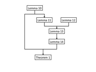
Figure 10: Diagram for lemmas and Theorem 28.

The proof of Theorem 28 requires several working lemmas. We provide a chart for how we are going to prove Theorem 28.

First, we define some notations about gradient flows. Recall that $\pi_{x}(t)\in\mathbb{K}$ is the gradient (ascent) flow starting at $x$:

$$\pi_{x}(0)=x,\quad\pi_{x}^{\prime}(t)=g(\pi_{x}(t)).$$

For $x$ that is not on the boundary set $D$, we define the time:

$$t_{\epsilon}(x)=\inf\{t:\pi_{x}(s)\in B(m,\sqrt{\epsilon}),\mbox{ for all}s\geq t\},$$

where $m$ is the destination of $\pi_{x}$. That is, $t_{\epsilon}(x)$ is the time to arrive the regions around a local mode.

First, we prove a property for the direction of the gradient field around boundaries.

Lemma 10 (Gradient field and boundaries)

Assume the notations in Theorem 28 and assume $f$ is a Morse function with bounded third derivatives and satisfies assumption (D). Let $s(x)=x-\Pi_{x}$, where $\Pi_{x}\in B$ is the projected point from $x$ onto $B$ (when $\Pi_{x}$ is not unique, just pick any projected point). For any $q\in B$, let $x$ be a point near $q$ such that $x-q\in\mathbb{V}(q)$, the normal space of $B$ at $q$. Let $\delta(x)=\|x-q\|$ and $e(x)=\frac{x-q}{\|x-q\|}$ denote the unit vector. Then

1. For every point $x$ such that

   $$d(x,B)\leq\delta_{1}=\frac{2H_{\min}}{d^{2}\cdot\|f\|_{3,\max}},$$

   we have

   $$g(x)^{T}s(x)\geq 0.$$

   That is, the gradient is pushing $x$ away from the boundaries.

2. When $\delta(x)\leq\frac{H_{\min}}{d^{2}\cdot\|f\|_{3,\max}}$,

   $$\ell(x)=e(x)^{T}g(x)\geq\frac{1}{2}H_{\min}\delta(x).$$

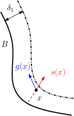
(a) Lemma 10

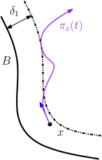
(b) Lemma 11

Figure 11: Illustration for Lemma 10 and 11. (a): We show that the angle between projection vector $s(x)$ and the gradient $g(x)$ is always right whenever $x$ is closed to the boundaries $B$. (b): According to (a), any gradient flow line start from a point $x$ that is close to the boundaries (distance $<\delta_{1}$), this flow line is always moving away from the boundaries when the current location is close to the boundaries. The flow line can temporally get closer to the boundaries when it is away from boundaries (distance $>\delta_{1}$)

Proof A.1.

Claim 1. Because the projection of $x$ onto $B$ is $\Pi_{x}$, $s(x)\in\mathbb{V}(\Pi_{x})$ and $s(x)^{T}g(\Pi_{x})=0$ (recall that for $p\in B$, $\mathbb{V}(p)$ is the collection of normal vectors of $B$ at $p$).

Recall that $d(x,B)=\|s(x)\|$ is the projected distance. By the fact that $s(x)^{T}g(\Pi_{x})=0$,

$$s(x)^{T}g(x) =s(x)^{T}(g(x)-g(\Pi_{x}))$$ (40)

$$\geq s(x)^{T}H(\Pi_{x})s(x)-\frac{d^{2}}{2}\|f\|_{3,\max}d(x,B)^{3}\quad\mbox{(Taylor's theorem)}$$

$$=d(x,B)^{2}\frac{s(x)^{T}}{d(x,B)}H(\Pi_{x})\frac{s(x)}{d(x,B)}-\frac{d^{2}}{2}\|f\|_{3,\max}d(x,B)^{3}$$

$$\geq d(x,B)^{2}\left(H_{\min}-\frac{d^{2}}{2}\|f\|_{3,\max}d(x,B)\right).$$

Note that we use the vector-value Taylor’s theorem in the first inequality and the fact that for two close points $x,y$, the difference in the $j$-the element of gradient $g_{j}(x)-g_{j}(y)$ has the following expansion

$$g_{j}(x)-g_{j}(y) =H_{j}(y)^{T}(x-y)+\int_{u=y}^{x}(u-y){\sf T}_{j}(u)du$$

$$\geq H_{j}(y)^{T}(x-y)-\frac{1}{2}\sup_{u}\|{\sf T}_{j}(u)\|_{2}\|x-y\|^{2}$$

$$\geq H_{j}(y)^{T}(x-y)-\frac{d^{2}}{2}\|f\|_{3,\max}\|x-y\|^{2},$$

where $H_{j}(y)=\nabla g_{j}(y)$ and ${\sf T}_{j}(y)=\nabla\nabla g_{j}(y)$ is the Hessian matrix of $g_{j}(y)$, whose elements are the third derivatives of $f(y)$.

Thus, when $d(x,B)\leq\frac{2H_{\min}}{d^{2}\cdot\|f\|_{3,\max}}$, $s(x)^{T}g(x)\geq 0$, which proves the first claim.

Claim 2. By definition, $e(x)^{T}g(q)=0$ because $g(q)$ is in tangent space of $B$ at $q$ and $e(x)$ is in the normal space of $B$ at $q$. Thus,

$$\ell(x) =e(x)^{T}g(x)$$ (41)

$$=e(x)^{T}\left(g(x)-g(q)\right)$$

$$\geq e(x)^{T}H(q)(x-q)-\frac{d^{2}}{2}\|f\|_{3,\max}\|x-q\|^{2}$$

$$=e(x)^{T}H(\pi(x))e(x)\delta(x)-\frac{d^{2}}{2}\|f\|_{3,\max}\delta(x)^{2}$$

$$\geq\frac{1}{2}H_{\min}\delta(x)$$

whenever $\delta(x)=\|x-q\|\leq\frac{H_{\min}}{d^{2}\cdot\|f\|_{3,\max}}$. Note that in the first inequality we use the same lower bound as the one in claim 1. Also note that $x-q=e(x)\delta(x)$ and $e(x)$ is in the normal space of $B$ at $\pi(x)$ so the third inequality follows from assumption (D).

Lemma 10 can be used to prove the following result.

Lemma 11 (Distance between flows and boundaries).

Assume the notations as the above and assumption (D). Then for all $x$ such that $0<d(x,B)=\delta\leq\delta_{1}=\frac{2H_{\min}}{d^{2}\|f\|_{3,\max}}$,

$$d(\pi_{x}(t),B)\geq\delta,$$

for all $t\geq 0$.

The main idea is that the projected gradient (gradient projected to the normal space of nearby boundaries) is always positive. This means that the flow cannot move “closer” to the boundaries.

Proof A.2.

By Lemma 10, for every point $x$ near to the boundaries ($d(x,B)<\delta_{1}$), the gradient is moving this point away from the boundaries. Thus, for any flow $\pi_{x}(t)$, once it touches the region $B\oplus\delta_{1},$ it will move away from this region. So when a flow leaves $B\oplus\delta_{1}$, it can never come back.

Therefore, the only case that a flow can be within the region $B\oplus\delta_{1}$ is that it starts at some $x\in B\oplus\delta_{1}$. i.e. $d(x,B)<\delta_{1}$.

Now consider a flow start at $x$ such that $0<d(x,B)\leq\delta_{1}$. By Lemma 10, the gradient $g(x)$ leads $x$ to move away from the boundaries $B$. Thus, whenever $\pi_{x}(t)\in B\oplus\delta_{1}$, the gradient is pushing $\pi_{x}(t)$ away from $B$. As a result, the time that $\pi_{x}(t)$ is closest to $B$ is at the beginning of the flow .i.e. $t=0$. This implies that $d(\pi_{x}(t),B)\geq d(\pi_{x}(0),B)=d(x,B)=\delta$.

With Lemma 11, we are able to bound the low gradient regions since the flow cannot move infinitely close to critical points except its destination. Let $\lambda_{\min}>0$ be the minimal ‘absolute’ value of eigenvalues of all critical points.

Lemma 12 (Bounds on low gradient regions).

Assume the density function $f$ is a Morse function and has bounded third derivatives. Let $\mathcal{C}$ denote the collection of all critical points and let $\lambda_{\min}$ is the minimal ‘absolute’ eigenvalue for Hessian matrix $H(x)$ evaluated at $x\in\mathcal{C}$. Then there exists a constant $\delta_{2}>0$ such that

$$G(\delta)\equiv\left\{x:\|g(x)\|\leq\frac{\lambda_{\min}}{2}\delta\right\}\subset\mathcal{C}\oplus\delta$$ (42)

for every $\delta\leq\delta_{2}$.

Proof A.3.

Because the support $\mathbb{K}$ is compact and $x\in\mathbb{K}\mapsto\|g(x)\|$ is continuous, for any $g_{0}>0$ sufficiently small, there exists a constant $R(g_{0})>0$ such that

$$G_{1}(g_{0})\equiv\left\{x:\|g(x)\|\leq g_{0}\right\}\subset\mathcal{C}\oplus R(g_{0})$$

and when $g_{0}\rightarrow 0$, $R(g_{0})\rightarrow 0$. Thus, there is a constant $g_{1}>0$ such that $R(g_{1})=\frac{\lambda_{\min}}{2d^{3}\|f\|_{3,\max}}$.

The set $\mathcal{C}\oplus\frac{\lambda_{\min}}{2\|f\|_{3,\max}}$ has a useful feature: for any $x\in\mathcal{C}\oplus\frac{\lambda_{\min}}{2\|f\|_{3,\max}}$,

$$\|H(x)-H(c)\|_{F} =\|(x-c)f^{(3)}(c+t(x-c))dt\|_{F}$$

$$\leq d^{3}\|x-c\|\|f\|_{3,\max}$$

$$\leq d^{3}\frac{\lambda_{\min}}{2d^{3}\|f\|_{3,\max}}\cdot\|f\|_{3,\max}$$

$$=\frac{\lambda_{\min}}{2},$$

where $f^{(3)}$ is a $d\times d\times d$ array of the third derivative of $f$ and $\|A\|_{F}$ is the Frobenius norm of the matrix A. By Hoffman–Wielandt theorem (see, e.g., page 165 of Bhatia 1997), the eigenvalues between $H(x)$ and $H(c)$ is bounded by $\|H(x)-H(c)\|_{F}$. Therefore, the smallest eigenvalue of $H(x)$ must be greater than or equal to the smallest eigenvalue of $H(c)$ minus $\frac{\lambda_{\min}}{2}$. Because $\lambda_{\min}$ is the smallest absolute eigenvalues of $H(c)$ for all $c\in{\cal C}$, the smallest eigenvalue of $H(x)$ is greater than or equal to $\frac{\lambda_{\min}}{2}$, for all $x\in\mathcal{C}\oplus R(g_{1})=\mathcal{C}\oplus\frac{\lambda_{\min}}{2d^{3}\|f\|_{3,\max}}$.

Using the above feature and the fact that $G_{1}(g_{1})\subset\mathcal{C}\oplus\frac{\lambda_{\min}}{2d^{3}\|f\|_{3,\max}}$, for any $x\in G_{1}(g_{1})$, we have the following inequalities:

$$g_{1} \geq\|g(x)\|$$

$$=\left\|\int_{0}^{1}(x-c)H(c+t(x-c))dt\right\|$$

$$\geq\|x-c\|\frac{1}{2}\lambda_{\min}.$$

Thus, $\|x-c\|\leq\frac{2g_{1}}{\lambda_{\min}}$, which implies

$$G_{1}(g_{1})\subset\mathcal{C}\oplus\frac{2g_{1}}{\lambda_{\min}}.$$

Moreover, because $G_{1}(g_{2})\subset G_{1}(g_{3})$ for any $g_{2}\leq g_{3}$, any $g_{2}\leq g_{1}$ satisfies

$$G_{1}(g_{2})\subset\mathcal{C}\oplus\frac{2g_{2}}{\lambda_{\min}}.$$

Now pick $\delta=\frac{2g_{2}}{\lambda_{\min}}$, we conclude

$$G_{1}\left(\frac{\lambda_{\min}}{2\delta}\right)=G(\delta)\subset\mathcal{C}\oplus\delta$$

for all

$$\delta=\frac{2g_{2}}{\lambda_{\min}}\leq\frac{2g_{1}}{\lambda_{\min}}=\delta_{2},$$ (43)

where $g_{1}$ is the constant such that $R(g_{1})=\frac{\lambda_{\min}}{2d^{3}\|f\|_{3,\max}}$.

Lemma 13 (Bounds on gradient flow).

Using the notations above and assumption (D), let $\delta_{1}$ be defined in Lemma 11 and $\delta_{2}$ be defined in Lemma 12, equation (43). Then for all $x$ such that

$$d(x,B)=\delta<\delta_{0}=\min\left\{\delta_{1},\delta_{2},\frac{H_{\min}}{d^{2}\cdot\|f\|_{3,\max}}\right\},$$

and picking $\epsilon$ such that $\delta_{2}>\epsilon^{2}>\delta$, we have

$$\eta_{\epsilon}(x)\equiv\underset{0\leq t\leq t_{\epsilon}(x)}{\inf}\|g(\pi_{x}(t))\|\geq\delta\frac{\lambda_{\min}}{2}.$$

Moreover,

$$\gamma_{\epsilon}(\delta)\equiv\underset{x\in B_{\delta}}{\inf}\eta_{\epsilon}(x)\geq\delta\frac{\lambda_{\min}}{2},$$

where $B_{\delta}=\{x:d(x,B)=\delta\}$.

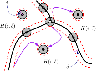
Figure 12: Illustration for $\mathcal{H}(\epsilon,\delta)$. The thick black lines are boundaries $B$; solid dots are local modes; box is local minimum; empty dots are saddle points. The three purple lines denote possible gradient flows starting from some points $x$ with $d(x,B)=\delta$. The gray disks denote all possible regions such that $\|g\|\leq\frac{\lambda_{\min}}{2}\delta$. Thus, the amount of gradient within the set $\mathcal{H}(\epsilon,\delta)$ is greater or equal to $\frac{\lambda_{\min}}{2}\delta$.

Proof A.4.

We consider the flow $\pi_{x}$ starting at $x$ (not on the boundaries) such that

$$d(x,B)=\delta<\min\left\{\delta_{1},\delta_{2}\right\}.$$

For $0\leq t\leq t_{\epsilon}(x)$, the entire flow is within the set

$$\mathcal{H}(\epsilon,\delta)=\{x:d(x,B)\geq\delta,d(x,M)\geq\sqrt{\epsilon}\}.$$ (44)

That is,

$$\{\pi_{x}(t):0\leq t\leq t_{\epsilon}(x)\}\subset\mathcal{H}(\epsilon,\delta).$$ (45)

This is because by Lemma 11, the flow line cannot get closer to the boundaries $B$ within distance $\delta$, and the flow stops when its distance to its destination is at $\epsilon$. Thus, if we can prove that every point within $\mathcal{H}(\epsilon,\delta)$ has gradient lowered bounded by $\delta\frac{\lambda_{\min}}{2}$, we have completed the proof. That is, we want to show that

$$\underset{x\in\mathcal{H}(\epsilon,\delta)}{\inf}\|g(x)\|\geq\delta\frac{\lambda_{\min}}{2}.$$ (46)

To show the lower bound, we focus on those points whose gradient is small. Let

$$S(\delta)=\left\{x:\|g(x)\|\leq\delta\frac{\lambda_{\min}}{2}\right\}.$$

By Lemma 12, the $S(\delta)$ are regions around critical points such that

$$S(\delta)\subset\mathcal{C}\oplus\delta.$$

Since we have chosen $\epsilon$ such that $\epsilon\geq\delta^{2}$ and by the fact that critical points are either in $M$, the collection of all local modes, or in $B$ the boundaries so that, the minimal distance between $\mathcal{H}(\epsilon,\delta)$ and critical points $\mathcal{C}$ is greater that $\delta$ (see equation (44) for the definition of $\mathcal{H}(\epsilon,\delta)$). Thus,

$$(\mathcal{C}\oplus\delta)\cap\mathcal{H}(\epsilon,\delta)=\emptyset,$$

which implies equation (46):

$$\underset{x\in\mathcal{H}(\epsilon,\delta)}{\inf}\|g(x)\|\geq\delta\frac{\lambda_{\min}}{2}.$$

Now by the fact that all $\pi_{x}(t)$ with $d(x,B)<\delta$ are within the set $\mathcal{H}(\epsilon,\delta)$ (equation (45)), we conclude the result.

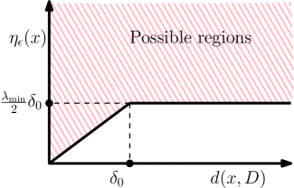
Figure 13: Result from Lemma 13: lower bound on minimal gradient. This plot shows possible values for minimal gradient $\eta_{\epsilon}(x)$ (pink regions) when $d(x,B)$ is known. Note that we have chosen $\epsilon^{2}<\delta_{2}$.

Lemma 13 links the constant $\gamma_{\epsilon}(\delta)$ and the minimal gradient, which can be used to bound the time $t_{\epsilon}(x)$ uniformly and further leads to the following result.

Lemma 14.

Let $\mathbb{K}(\delta)=\{x\in\mathbb{K}:d(x,B)\geq\delta\}=\mathbb{K}\backslash(B\oplus\delta)$ and $\delta_{0}$ be defined as Lemma 13 and $M$ is the collection of all local modes. Assume that $f$ has bounded third derivative and is a Morse function and that assumption (D) holds. Let $\widetilde{f}$ be another smooth function. There exists constants $c_{*},c_{0},c_{1},\epsilon_{0}$ that all depend only on $f$ such that when $(\epsilon,\delta)$ satisfy the following condition

$$\delta<\epsilon<\epsilon_{0},\quad\delta<\min\{\delta_{0},{\sf Haus}(\mathbb{K}(\delta),B(M,\sqrt{\epsilon}))\}$$ (47)

and if

$$\|f-\widetilde{f}\|^{*}_{3,\max} \leq c_{0}$$ (48)

$$\|f-\widetilde{f}\|_{1,\max} \leq c_{1}\exp\left(-\frac{4\sqrt{d}\|f\|_{2,\max}\|f\|_{\infty}}{\delta^{2}\lambda^{2}_{\min}}\right),$$

then for all $x\in\mathbb{K}(\delta)$

$$\|\lim_{t\rightarrow\infty}\pi_{x}(t)-\lim_{t\rightarrow\infty}\widetilde{\pi}_{x}(t)\|\leq c_{*}\sqrt{\|f-\widetilde{f}\|_{\infty}}.$$ (49)

Note that condition (47) holds when $(\epsilon,\delta)$ are sufficiently small.

Proof A.5.

The proof of this lemma is closely related to the proof of Theorem 2 of Arias-Castro et al. (2016). The results in Arias-Castro et al. (2016) is a pointwise convergence of gradient flows; now we will generalize their findings to the uniform convergence.

Note that $\mathbb{K}(\delta)=\mathcal{H}(\epsilon,\delta)\cup B(x,\sqrt{\epsilon})$. For $x\in B(x,\sqrt{\epsilon})$, the result is trivial when $\epsilon$ is sufficiently small. Thus, we assume $x\in\mathcal{H}(\epsilon,\delta)$.

From equation (40–44) in Arias-Castro et al. (2016) (proof to their Theorem 2),

$$\|\lim_{t\rightarrow\infty} \pi_{x}(t)-\lim_{t\rightarrow\infty}\widetilde{\pi}_{x}(t)\|$$ (50)

$$\leq\sqrt{\frac{2}{\lambda_{\min}}\left(2\lambda_{\min}\epsilon+\frac{\|f\|_{1,\max}}{\sqrt{d}\|f\|_{2,\max}}\|f-\widetilde{f}\|_{1,\max}e^{\sqrt{d}\|f\|_{2,\max}t_{\epsilon}(x)}+2\|f-\widetilde{f}\|_{\infty}\right)}$$

under condition (48) and $\epsilon<\epsilon_{0}$ for some constant $\epsilon_{0}$.

Thus, the key is to bound $t_{\epsilon}(x)$. Recall that $x\in\mathcal{H}(\epsilon,\delta)$. Now consider the gradient flow $\pi_{x}$ and define $z=\pi_{x}(t_{\epsilon}(x))$.

$$f(z)-f(x) =\int_{0}^{t_{\epsilon}(x)}\frac{\partial f(\pi_{x}(s))}{\partial s}ds=\int_{0}^{t_{\epsilon}(x)}g(\pi_{x}(s))^{T}\pi^{\prime}_{x}(s)ds$$ (51)

$$=\int_{0}^{t_{\epsilon}(x)}\|g(\pi_{x}(s))\|^{2}ds\geq\gamma_{\epsilon}(\delta)^{2}t_{\epsilon}(x).$$

Since $f(z)-f(x)\leq 2\|f\|_{\infty}$, we have

$$\|f\|_{\infty}\geq\frac{1}{2}\gamma_{\epsilon}(\delta)^{2}t_{\epsilon}(x)$$

and by Lemma 13,

$$t_{\epsilon}(x)\leq\frac{2\|f\|_{\infty}}{\gamma_{\epsilon}(\delta)^{2}}\leq\frac{8\|f\|_{\infty}}{\delta^{2}\lambda^{2}_{\min}}$$ (52)

for all $x\in\mathcal{H}(\epsilon,\delta)$.

Now plug-in (52) into (50), we have

$$\|\lim_{t\rightarrow\infty}\pi_{x}(t)-\lim_{t\rightarrow\infty}\widetilde{\pi}_{x}(t)\|\leq\sqrt{a_{0}\epsilon+a_{1}\|f-\widetilde{f}\|_{1,\max}e^{\sqrt{d}\|f\|_{2,\max}\frac{8\|f\|_{\infty}}{\delta^{2}\lambda^{2}_{\min}}}+a_{2}\|f-\widetilde{f}\|_{\infty}}$$ (53)

for some constants $a_{0},a_{1},a_{2}$. Now using condition (48) to replace the second term of right hand side, we conclude

$$\|\lim_{t\rightarrow\infty}\pi_{x}(t)-\lim_{t\rightarrow\infty}\widetilde{\pi}_{x}(t)\|\leq a_{3}\sqrt{\epsilon+\|f-\widetilde{f}\|^{*}_{1,\max}}$$

for some constant $a_{3}$.

By Lemma 7 in Arias-Castro et al. (2016), there exists some constant $c_{3}$ such that when $a_{3}\sqrt{\epsilon+\|f-\widetilde{f}\|^{*}_{1,\max}}<1/c_{3}$,

$$\|\lim_{t\rightarrow\infty}\pi_{x}(t)-\lim_{t\rightarrow\infty}\widetilde{\pi}_{x}(t)\|\leq\sqrt{2}c_{3}\|f-\widetilde{f}\|.$$

Thus, when both $\epsilon$ and $\|f-\widetilde{f}^{*}_{3,\max}\|$ are sufficiently small, there exists some constant $c_{*}$ such that

$$\|\lim_{t\rightarrow\infty}\pi_{x}(t)-\lim_{t\rightarrow\infty}\widetilde{\pi}_{x}(t)\|\leq c_{*}\|f-\widetilde{f}\|$$

for all $x\in\mathcal{H}(\epsilon,\delta)$.

Now we turn to the proof of Theorem 28.

Proof A.6 ( of Theorem 28).

The proof contains two parts. In the first part, we show that when $\|f-\widetilde{f}\|^{*}_{3,\max}$ is sufficiently small, we have ${\sf Haus}(B,\widetilde{B})<\frac{H_{\min}}{d^{2}\|f\|_{3,\max}}$, where $B$ and $\widetilde{B}$ are the boundary of descending $d$-manifolds for $f$ and $\widetilde{f}$. The second part of the proof is to derive the convergence rate. Because ${\sf Haus}(B,\widetilde{B})<\frac{H_{\min}}{d^{2}\|f\|_{3,\max}}$, we can apply the second assertion of Lemma 10 to derive the rate of convergence. Note that ${\cal C}$ and $\widetilde{{\cal C}}$ are the critical points for $f$ and $\widetilde{f}$ and $M\equiv C_{0}$, $\widetilde{M}\equiv\widetilde{C}_{0}$ are the local modes for $f$ and $\widetilde{f}$.

Part 1: ${\sf Haus}(B,\widetilde{B})<\frac{H_{\min}}{d^{2}\cdot\|f\|_{3,\max}}$, the upper bound for Hausdorff distance. Let $\sigma=\min\{\|x-y\|:x,y\in M,x\neq y\}$. That is, $\sigma$ is the smallest distance between any pair of distinct local modes. By Lemma 9, when $\|f-\widetilde{f}\|^{*}_{3,\max}$ is small, $f$ and $\widetilde{f}$ have the same number of critical points and

$${\sf Haus}({\cal C},\widetilde{{\cal C}})\leq A\|f-\widetilde{f}\|^{*}_{2,\max}\leq A\|f-\widetilde{f}\|^{*}_{3,\max},$$

where $A$ is a constant that depends only on $f$ (actually, we only need $\|f-\widetilde{f}\|^{*}_{2,\max}$ to be small here).

Thus, whenever $\|f-\widetilde{f}\|^{*}_{3,\max}$ satisfies

$$\|f-\widetilde{f}\|^{*}_{3,\max}\leq\frac{\sigma}{3A},$$ (54)

every $M$ has an unique corresponding point in $\widetilde{M}$ and vice versa. In addition, for a pair of local modes $(m_{j},\widetilde{m}_{j}):m_{j}\in M,\widetilde{m}_{j}\in\widetilde{M}$, their distance is bounded by $\|m_{j}-\widetilde{m}_{j}\|\leq\frac{\sigma}{3}$.

Now we pick $(\epsilon,\delta)$ such that they satisfy equation (47). Then when $\|f-\widetilde{f}\|^{*}_{3,\max}$ is sufficiently small, by Lemma 49, for every $x\in\mathcal{H}(\epsilon,\delta)$ we have

$$\|\lim_{t\rightarrow\infty}\pi_{x}(t)-\lim_{t\rightarrow\infty}\widetilde{\pi}_{x}(t)\|\leq c_{*}\sqrt{\|f-\widetilde{f}\|_{\infty}}\leq c_{*}\sqrt{\|f-\widetilde{f}\|^{*}_{3,\max}}.$$

Thus, whenever

$$\|f-\widetilde{f}\|^{*}_{3,\max}\leq\frac{1}{c^{2}_{*}}\left(\frac{\sigma}{3}\right)^{2},$$ (55)

$\pi_{x}(t)$ and $\widetilde{\pi}_{x}(t)$ leads to the same pair of modes. Namely, the boundaries $\widetilde{B}$ will not intersect the region $\mathcal{H}(\epsilon,\delta)$. And it is obvious that $\widetilde{B}$ cannot intersect $B(M,\sqrt{\epsilon})$. To conclude,

$$\widetilde{B}\cap\mathcal{H}(\epsilon,\delta) =\emptyset$$ (56)

$$\widetilde{B}\cap B(M,\sqrt{\epsilon}) =\emptyset$$

$$\Rightarrow\widetilde{B}\cap\mathbb{K}(\delta) =\emptyset,$$

because by definition, $\mathbb{K}(\delta)=\mathcal{H}(\epsilon,\delta)\cap B(M,\sqrt{\epsilon})$.

Thus, $\widetilde{B}\subset\mathbb{K}(\delta)^{C}=B\oplus\delta$, which implies ${\sf Haus}(B,\widetilde{B})\leq\delta<\frac{H_{\min}}{d^{2}\|f\|_{3,\max}}$ (note that $\delta<\delta_{0}\leq\frac{H_{\min}}{d^{2}\|f\|_{3,\max}}$ appears in equation (47) and Lemma 13).

Part 2: Rate of convergence. To derive the convergence rate, we use proof by contradiction. Let $q\in B,\widetilde{q}\in\widetilde{B}$ a pair of points such that their distance attains the Hausdorff distance ${\sf Haus}\left(\widetilde{B},B\right)$. Namely, $q$ and $\widetilde{q}$ satisfy

$$\|q-\widetilde{q}\|={\sf Haus}\left(\widetilde{B},B\right)$$

and either $q$ is the projected point from $\widetilde{q}$ onto $B$ or $\widetilde{q}$ is the projected point from $q$ onto $\widetilde{B}$.

Recall that $\mathbb{V}(x)$ is the normal space to $B$ at $x\in B$ and we define $\widetilde{\mathbb{V}}(x)$ similarly for $x\in\widetilde{B}$. An important property of the pair $q,\widetilde{q}$ is that $q-\widetilde{q}\in\mathbb{V}(q),\widetilde{\mathbb{V}}(\widetilde{q})$. If this is not true, we can slightly perturb $q$ (or $\widetilde{q}$) on $B$ (or $\widetilde{B}$) to get a projection distance larger than the Hausdorff distance, which leads to a contradiction.

Now we choose $x$ to be a point between $q,\widetilde{q}$ such that $x=\frac{1}{3}q+\frac{2}{3}\widetilde{q}$. We define $e(x)=\frac{q-x}{\|q-x\|}$ and $\widetilde{e}(x)=\frac{\widetilde{q}-x}{\|\widetilde{q}-x\|}$. Then $e(x)\in\mathbb{V}(q)$ and $\widetilde{e}(x)\in\widetilde{\mathbb{V}}(\widetilde{q})$ and $e(x)=-\widetilde{e}(x)$.

By Lemma 10 (second assertion),

$$\ell(x) =e(x)^{T}g(x)\geq\frac{1}{2}H_{\min}\|q-x\|>0$$ (57)

$$\widetilde{\ell}(x) =\widetilde{e}(x)^{T}\widetilde{g}(x)\geq\frac{1}{2}\widetilde{H}_{\min}\|\widetilde{q}-x\|>0.$$

Thus, for every $x$ between $q,\widetilde{q}$,

$$e(x)^{T}g(x)>0,\quad,e(x)^{T}\widetilde{g}(x)=-\widetilde{e}(x)^{T}\widetilde{g}(x)<0.$$ (58)

Note that we can apply Lemma 10 to $\widetilde{f}$ and its gradient because when $\|f-\widetilde{f}\|^{*}_{2}$ is sufficiently small, the assumption (D) holds for $\widetilde{f}$ as well.

To get the upper bound of $\|q-\widetilde{q}\|={\sf Haus}(\widetilde{B},B)$, note that $\|q-x\|=\frac{2}{3}\|q-\widetilde{q}\|$, so

$$e(x)^{T}\widetilde{g}(x) =e(x)^{T}(\widetilde{g}(x)-g(x))+e(x)^{T}g(x)$$ (59)

$$\geq e(x)^{T}g(x)-\|\widetilde{f}-f\|_{1,\max}$$

$$\geq\frac{1}{2}H_{\min}\|q-x\|-\|\widetilde{f}-f\|_{1,\max}\quad\mbox{(By Lemma \ref{lem::Gdist})}$$

$$=\frac{1}{3}H_{\min}\|q-\widetilde{q}\|-\|\widetilde{f}-f\|_{1,\max}.$$

Thus, as long as

$${\sf Haus}(\widetilde{B},B)=\|q-\widetilde{q}\|>3\frac{\|\widetilde{f}-f\|_{1,\max}}{H_{\min}},$$

we have $e(x)^{T}\widetilde{g}(x)>0$, a contradiction to equation (58). Hence, we conclude that

$${\sf Haus}(\widetilde{B},B)\leq 3\frac{\|\widetilde{f}-f\|_{1,\max}}{H_{\min}}=O\left(\|\widetilde{f}-f\|_{1,\max}\right).$$

Proof A.7 ( of Theorem 3).

To prove the asymptotic rate of the rand index, we assume that for every local mode of $p$, there exists one and only one local mode of $\widehat{p}_{n}$ that is close to the specific mode of $p$. By Lemma 9, this is true when $\|\widehat{p}_{n}-p\|^{*}_{3,\max}$ is sufficiently small. Thus, after relabeling, the local mode $\widehat{m}_{\ell}$ of $\widehat{p}_{n}$ is an estimator to the local mode $m_{\ell}$ of $p$. Let $\widehat{W}_{\ell}$ be the basin of attraction to $\widehat{m}_{\ell}$ using $\nabla\widehat{p}_{n}$ and $W_{\ell}$ be the basin of attraction to $m_{\ell}$ using $\nabla p$. Let $A\triangle B=\{x:x\in A,x\notin B\}\cup\{x:x\in B,x\notin A\}$ be the symmetric difference between sets $A$ and $B$. The regions

$$E_{n}=\bigcup_{\ell}\left(\widehat{W}_{\ell}\triangle W_{\ell}\right)\subset\mathbb{K}$$ (60)

are where the two mode clustering disagree with each other. Note that $E_{n}$ are regions between the two boundaries $\widehat{B}_{n}$ and $B$

Given a pair of points $X_{i}$ and $X_{j}$,

$$\Psi(X_{i},X_{j})\neq\widehat{\Psi}_{n}(X_{i},X_{j})\Longrightarrow X_{i}\mbox{ or }X_{j}\in E_{n}.$$ (61)

By the definition of rand index (30),

$$1-{\sf rand}\left(\widehat{p}_{n},p\right)={n\choose 2}^{-1}\sum_{i,j}1\left(\Psi(X_{i},X_{j})\neq\widehat{\Psi}_{n}(X_{i},X_{j})\right)$$ (62)

Thus, if we can bound the ratio of data points within $E_{n}$, we can bound the rate of rand index.

Since $\mathbb{K}$ is compact and $p$ has bounded second derivatives, the volume of $E_{n}$ is bounded by

$${\sf Vol}(E_{n})=O\left({\sf Haus}(\widehat{B}_{n},B)\right).$$ (63)

Note ${\sf Vol}(A)$ denotes the volume (Lebesgue measure) of a set $A$. We now construct a region surrounding $B$ such that

$$E_{n}\subset B\oplus{\sf Haus}(\widehat{B}_{n},B)=V_{n}$$ (64)

and

$${\sf Vol}(V_{n})=O\left({\sf Haus}(\widehat{B}_{n},B)\right).$$ (65)

Now we consider a collection of subsets of $\mathbb{K}$:

$$\mathcal{V}=\{B\oplus r:R>r>0\},$$ (66)

where $R<\infty$ is the diameter for $\mathbb{K}$. For any set $A\subset\mathbb{K}$, let $P(X_{i}\in A)$ and $\widehat{P}_{n}(A)=\frac{1}{n}\sum_{i=1}^{n}1(X_{i}\in A)$ denote the probability of an observation within $A$ and the empirical estimate for that probability, respectively. It is easy to see that $V_{n}\in\mathcal{V}$ for all $n$ and the class $\mathcal{V}$ has a finite VC dimension (actually, the VC dimension is $1$). By the empirical process theory (or so-called VC theory, see e.g. Vapnik and Chervonenkis (1971)),

$$\underset{A\in\mathcal{V}}{\sup}\left|P(X_{i}\in A)-\widehat{P}_{n}(A)\right|=O_{\mathbb{P}}\left(\sqrt{\frac{\log(n)}{n}}\right).$$ (67)

Thus,

$$\left|P(X_{i}\in V_{n})-\widehat{P}_{n}(V_{n})\right|=O_{\mathbb{P}}\left(\sqrt{\frac{\log(n)}{n}}\right).$$ (68)

Now by equations (61) and (62),

$$1-{\sf rand}\left(\widehat{p}_{n},p\right)\leq 8\widehat{P}_{n}(E_{n})\leq 8\widehat{P}_{n}(V_{n})\leq 8P(X_{i}\in V_{n})+O_{\mathbb{P}}\left(\sqrt{\frac{\log(n)}{n}}\right).$$ (69)

Therefore,

$$1-{\sf rand}\left(\widehat{p}_{n},p\right) \leq P(X_{i}\in V_{n})+O_{\mathbb{P}}\left(\sqrt{\frac{\log(n)}{n}}\right)$$ (70)

$$\leq\sup_{x\in\mathbb{K}}p(x)\times{\sf Vol}(V_{n})+O_{\mathbb{P}}\left(\sqrt{\frac{\log(n)}{n}}\right)$$

$$\leq O\left({\sf Haus}(\widehat{B}_{n},B)\right)+O_{\mathbb{P}}\left(\sqrt{\frac{\log(n)}{n}}\right)$$

$$=O\left(h^{2}\right)+O_{\mathbb{P}}\left(\sqrt{\frac{\log(n)}{nh^{d+2}}}\right),$$

which completes the proof. Note that we apply Theorem 2 in the last equality.

Proof A.8 ( of Theorem 4).

Let $(X_{1},Y_{1}),\cdots,(X_{n},Y_{n})$ be the observed data. Let $\widehat{E}_{\ell}$ denote the $d$-cell for the nonparametric pilot regression estimator $\widehat{m}_{n}$. With $I_{\ell}=\{i:X_{i}\in\widehat{E}_{\ell}\}$, we define $\mathbb{X}_{\ell}$ as the matrix with rows $X_{i}$, $i\in I_{\ell}$ and similarly we define $\mathbb{Y}_{\ell}$.

We define $\mathbb{X}_{0,\ell}$ to be the matrix similar to $\mathbb{X}_{\ell}$ except that the row elements are those $X_{i}$ within $E_{\ell}$, the $d$-cell defined on true regression function $m$. We also define $\mathbb{Y}_{0,\ell}$ to be the corresponding $Y_{i}$.

By the theory of linear regression, the estimated parameters $\widehat{\mu}_{\ell},\widehat{\beta}_{\ell}$ have a closed form solution:

$$(\widehat{\mu}_{\ell},\widehat{\beta}_{\ell})^{T}=(\mathbb{X}_{\ell}^{T}\mathbb{X}_{\ell})^{-1}\mathbb{X}_{\ell}^{T}\mathbb{Y}_{\ell}.$$ (71)

Similarly, we define

$$(\widehat{\mu}_{0,\ell},\widehat{\beta}_{0,\ell})^{T}=(\mathbb{X}_{0,\ell}^{T}\mathbb{X}_{0,\ell})^{-1}\mathbb{X}_{0,\ell}^{T}\mathbb{Y}_{0,\ell}$$ (72)

as the estimated coefficients using $\mathbb{X}_{0,\ell}$ and $\mathbb{Y}_{0,\ell}$.

As $\|\widetilde{m}-m\|^{*}_{3,\max}$ is small, by Theorem 3, the number of rows at which $\mathbb{X}_{\ell}$ and $\mathbb{X}_{0,\ell}$ differ is bounded by $O(n\times\|\widehat{m}_{n}-m\|_{1,\max})$. This is because an observation (a row vector) that appears only in one of $\mathbb{X}_{\ell}$ and $\mathbb{X}_{0,\ell}$ is those fallen within either $\widehat{E}_{\ell}$ or $E_{\ell}$ but not both. Despite the fact that Theorem 3 is for basins of attraction (d-descending manifolds) of local modes, it can be easily generalized to $0$-ascending manifolds of local minima under assumption (A). Thus, the similar bound holds for d-cells as well. Thus, we conclude that

$$\left\|\frac{1}{n}\mathbb{X}_{\ell}^{T}\mathbb{X}_{\ell}-\frac{1}{n}\mathbb{X}_{0,\ell}^{T}\mathbb{X}_{0,\ell}\right\|_{\infty} =O(\|\widehat{m}_{n}-m\|_{1,\max})$$ (73)

$$\left\|\frac{1}{n}\mathbb{X}_{\ell}^{T}\mathbb{Y}_{\ell}-\frac{1}{n}\mathbb{X}_{0,\ell}^{T}\mathbb{Y}_{0,\ell}\right\|_{\infty} =O(\|\widehat{m}_{n}-m\|_{1,\max})$$

since $(\mathbb{X}_{\ell},\mathbb{Y}_{\ell})$ and $(\mathbb{X}_{0,\ell},\mathbb{Y}_{0,\ell})$ only differ by $O(n\times\|\widehat{m}_{n}-m\|_{1,\max})$ elements. Thus,

$$\left\|(\widehat{\mu}_{0,\ell}-\widehat{\mu}_{\ell},\widehat{\beta}_{0,\ell}-\widehat{\beta}_{\ell})\right\|_{\infty} =\left\|\left(\frac{1}{n}\mathbb{X}_{0,\ell}^{T}\mathbb{X}_{0,\ell}\right)^{-1}\frac{1}{n}\mathbb{X}_{0,\ell}^{T}\mathbb{Y}_{0,\ell}-\left(\frac{1}{n}\mathbb{X}_{\ell}^{T}\mathbb{X}_{\ell}\right)^{-1}\frac{1}{n}\mathbb{X}_{\ell}^{T}\mathbb{Y}_{\ell}\right\|_{\infty}$$ (74)

$$=O(\|\widehat{m}_{n}-m\|_{1,\max}),$$

which implies.

$$\max\left\{\|\widehat{\mu}_{0,\ell}-\widehat{\mu}_{\ell}\|,\|\widehat{\beta}_{0,\ell}-\widehat{\beta}_{\ell}\|\right\}=O(\|\widehat{m}_{n}-m\|_{1,\max}).$$ (75)

Now by the theory of linear regression,

$$\max\left\{\|\widehat{\mu}_{0,\ell}-\mu_{\ell}\|,\|\widehat{\beta}_{0,\ell}-\beta_{\ell}\|\right\}=O_{\mathbb{P}}\left(\frac{1}{\sqrt{n}}\right).$$ (76)

Thus, combining (75) and (76) and use the fact that all the above bounds are uniform over each cell, we have proved that the parameters converge at rate $O(\|\widehat{m}_{n}-m\|_{1,\max})+O_{\mathbb{P}}\left(\frac{1}{\sqrt{n}}\right)$.

For points within the regions where $E_{\ell}$ and $\widehat{E}_{\ell}$ agree with each other, the rate of convergence for parameter estimation translates into the rate of $\widehat{m}_{n,{\sf MSR}}-m_{{\sf MSR}}$. The regions that $E_{\ell}$ and $\widehat{E}_{\ell}$ disagree to each other, denoted as $\mathbb{N}_{n}$, have Lebesgue $O(\|\widehat{m}_{n}-m\|_{1,\max})$ by Theorem 28. Thus, we have completed the proof.

Proof A.9 ( of Theorem 38).

The proof of Theorem 38 is nearly identical to the proof of Theorem 4. The only difference is that the number of rows that $\mathbb{X}_{\ell}$ and $\mathbb{X}_{0,\ell}$ differ is bounded by $O(n\times\|\widehat{m}_{n}-m\|_{1,\max}^{\beta})$ due to the low noise condition (36). Thus, equation (73) becomes

$$\left\|\frac{1}{n}\mathbb{X}_{\ell}^{T}\mathbb{X}_{\ell}-\frac{1}{n}\mathbb{X}_{0,\ell}^{T}\mathbb{X}_{0,\ell}\right\|_{\infty} =O(\|\widehat{m}_{n}-m\|_{1,\max}^{\beta})$$ (77)

$$\left\|\frac{1}{n}\mathbb{X}_{\ell}^{T}\mathbb{Y}_{\ell}-\frac{1}{n}\mathbb{X}_{0,\ell}^{T}\mathbb{Y}_{0,\ell}\right\|_{\infty} =O(\|\widehat{m}_{n}-m\|_{1,\max}^{\beta})$$

so the parameter estimation error (76) is $O(\|\widehat{m}_{n}-m\|_{1,\max}^{\beta})+O_{\mathbb{P}}\left(\frac{1}{\sqrt{n}}\right)$.

Under assumption (K1–2) and using Theorem 8 (the same result works for kernel regression),

$$O(\|\widehat{m}_{n}-m\|_{1,\max})=O(h^{2})+O_{\mathbb{P}}\left(\sqrt{\frac{\log n}{nh^{d+2}}}\right).$$

Thus, with the choice that $h=O\left(\left(\frac{\log n}{n}\right)^{1/(d+6)}\right)$, we have $O(\|\widehat{m}_{n}-m\|_{1,\max})=O_{\mathbb{P}}\left(\left(\frac{\log n}{n}\right)^{2/(d+6)}\right)$, which proves equation (37).

Proof A.10 ( of Theorem 6).

We first derive the explicit form of the parameters $(\eta^{\dagger}_{\ell},\gamma^{\dagger}_{\ell})$ within cell $E_{\ell}$. Note that the parameters are obtained by (14):

$$(\eta_{\ell}^{\dagger},\gamma_{\ell}^{\dagger})=\underset{\eta,\gamma}{\sf argmin}\,\,\int_{E_{\ell}}\left(f(x)-\eta-\gamma^{T}x\right)^{2}dx.$$

Now we define a random variable $U_{\ell}\in\mathbb{R}^{d}$ that is uniformly distributed over $E_{\ell}$. Then equation (14) is equivalent to

$$(\eta_{\ell}^{\dagger},\gamma_{\ell}^{\dagger})=\underset{\eta,\gamma}{\sf argmin}\,\,\mathbb{E}\left(\left(f(U_{\ell})-\eta-\gamma^{T}U_{\ell}\right)^{2}\right).$$ (78)

The analytical solution to the above problem is

$$\left(\begin{array}[]{c}\eta^{\dagger}_{\ell}\\ \gamma^{\dagger}_{\ell}\end{array}\right)=\left(\begin{array}[]{cc}1&\mathbb{E}(U_{\ell})^{T}\\ \mathbb{E}(U_{\ell})&\mathbb{E}(U_{\ell}U_{\ell}^{T})\end{array}\right)^{-1}\left(\begin{array}[]{c}\mathbb{E}(f(U_{\ell}))\\ \mathbb{E}(U_{\ell}f(U_{\ell}))\end{array}\right)$$ (79)

Now we consider another smooth function $\widetilde{f}$ that is close to $f$ such that $\|\widetilde{f}-f\|^{*}_{3,\max}$ is small so we can apply Theorem 28 to obtain consistency for both descending $d$-manifolds and ascending $0$-manifolds. Note that by Lemma 9, all the critical points are close to each other and after relabeling, each $d$-cell $E_{\ell}$ of $f$ is estimated by another $d$-cell $\widetilde{E}_{\ell}$ of $\widetilde{f}$. Theorem 28 further implies that

$$\left|{\sf Leb}(\widetilde{E}_{\ell})-{\sf Leb}(E_{\ell})\right| =O\left(\|\widetilde{f}-f\|_{1,\max}\right)$$ (80)

$${\sf Leb}\left(\widetilde{E}_{\ell}\triangle E_{\ell}\right) =O\left(\|\widetilde{f}-f\|_{1,\max}\right),$$

where ${\sf Leb}(A)$ is the Lebesgue measure for set $A$ and $A\triangle B=(A\backslash B)\cup(B\backslash A)$ is the symmetric difference. By simple algebra, equation (80) implies that

$$\|\mathbb{E}(\widetilde{U}_{\ell}) -\mathbb{E}(U_{\ell})\|_{\infty}=O\left(\|\widetilde{f}-f\|_{1,\max}\right)$$ (81)

$$\|\mathbb{E}(\widetilde{U}_{\ell}\widetilde{U}_{\ell}^{T}) -\mathbb{E}(U_{\ell}U_{\ell}^{T})\|_{\infty}=O\left(\|\widetilde{f}-f\|_{1,\max}\right)$$

$$|\mathbb{E}(\widetilde{f}(\widetilde{U}_{\ell})) -\mathbb{E}(f(U_{\ell}))|=O\left(\|\widetilde{f}-f\|^{*}_{1,\max}\right)$$

$$\|\mathbb{E}(\widetilde{U}_{\ell}\widetilde{f}(\widetilde{U}_{\ell})) -\mathbb{E}(U_{\ell}f(U_{\ell}))\|_{\infty}=O\left(\|\widetilde{f}-f\|^{*}_{1,\max}\right).$$

By (81) and the analytic solution to $(\widetilde{\eta}^{\dagger}_{\ell},\widetilde{\gamma}^{\dagger}_{\ell})$ from (79), we have proved

$$\left\|\left(\begin{array}[]{c}\widetilde{\eta}^{\dagger}_{\ell}\\ \widetilde{\gamma}^{\dagger}_{\ell}\end{array}\right)-\left(\begin{array}[]{c}\eta^{\dagger}_{\ell}\\ \gamma^{\dagger}_{\ell}\end{array}\right)\right\|_{\infty}=O\left(\|\widetilde{f}-f\|^{*}_{1,\max}\right).$$ (82)

Since the bound does not depend on the cell indices $\ell$, (82) holds uniformly for all $\ell=1,\cdots,K$.

References

- Arias-Castro et al. (2016) E. Arias-Castro, D. Mason, and B. Pelletier. On the estimation of the gradient lines of a density and the consistency of the mean-shift algorithm. Journal of Machine Learning Research, 17(43):1–28, 2016.
- Audibert et al. (2007) J.-Y. Audibert, A. B. Tsybakov, et al. Fast learning rates for plug-in classifiers. The Annals of statistics, 35(2):608–633, 2007.
- Azizyan et al. (2015) M. Azizyan, Y.-C. Chen, A. Singh, and L. Wasserman. Risk bounds for mode clustering. arXiv preprint arXiv:1505.00482, 2015.
- Azzalini and Torelli (2007) A. Azzalini and N. Torelli. Clustering via nonparametric density estimation. Statistics and Computing, 17(1):71–80, 2007.
- Bacchetti (1989) P. Bacchetti. Additive isotonic models. Journal of the American Statistical Association, 84(405):289–294, 1989.
- Banyaga and Hurtubise (2004) A. Banyaga and D. Hurtubise. Lectures on Morse homology, volume 29. Springer Science & Business Media, 2004.
- Baringhaus and Franz (2004) L. Baringhaus and C. Franz. On a new multivariate two-sample test. Journal of multivariate analysis, 88(1):190–206, 2004.
- Barlow et al. (1972) R. E. Barlow, D. J. Bartholomew, J. Bremner, and H. D. Brunk. Statistical inference under order restrictions: the theory and application of isotonic regression. Wiley New York, 1972.
- Bhatia (1997) R. Bhatia. Matrix Analysis. Springer, 1997.
- Bredon (1993) G. E. Bredon. Topology and geometry, volume 139. Springer Science & Business Media, 1993.
- Brinkman et al. (2007) R. R. Brinkman, M. Gasparetto, S.-J. J. Lee, A. J. Ribickas, J. Perkins, W. Janssen, R. Smiley, and C. Smith. High-content flow cytometry and temporal data analysis for defining a cellular signature of graft-versus-host disease. Biology of Blood and Marrow Transplantation, 13(6):691–700, 2007.
- Chacón and Duong (2013) J. Chacón and T. Duong. Data-driven density derivative estimation, with applications to nonparametric clustering and bump hunting. Electronic Journal of Statistics, 7:499–532, 2013.
- Chacón et al. (2011) J. Chacón, T. Duong, and M. Wand. Asymptotics for general multivariate kernel density derivative estimators. Statistica Sinica, 2011.
- Chacón et al. (2015) J. E. Chacón et al. A population background for nonparametric density-based clustering. Statistical Science, 30(4):518–532, 2015.
- Chazal et al. (2014) F. Chazal, B. T. Fasy, F. Lecci, B. Michel, A. Rinaldo, and L. Wasserman. Robust topological inference: Distance to a measure and kernel distance. arXiv preprint arXiv:1412.7197, 2014.
- Chen et al. (2015) Y.-C. Chen, C. R. Genovese, L. Wasserman, et al. Asymptotic theory for density ridges. The Annals of Statistics, 43(5):1896–1928, 2015.
- Chen et al. (2016) Y.-C. Chen, C. R. Genovese, L. Wasserman, et al. A comprehensive approach to mode clustering. Electronic Journal of Statistics, 10(1):210–241, 2016.
- Cheng (1995) Y. Cheng. Mean shift, mode seeking, and clustering. Pattern Analysis and Machine Intelligence, IEEE Transactions on, 17(8):790–799, 1995.
- Cohen-Steiner et al. (2007) D. Cohen-Steiner, H. Edelsbrunner, and J. Harer. Stability of persistence diagrams. Discrete & Computational Geometry, 37(1):103–120, 2007.
- Comaniciu and Meer (2002) D. Comaniciu and P. Meer. Mean shift: A robust approach toward feature space analysis. Pattern Analysis and Machine Intelligence, IEEE Transactions on, 24(5):603–619, 2002.
- Duong (2013) T. Duong. Local significant differences from nonparametric two-sample tests. Journal of Nonparametric Statistics, 25(3):635–645, 2013.
- Duong et al. (2007) T. Duong et al. ks: Kernel density estimation and kernel discriminant analysis for multivariate data in r. Journal of Statistical Software, 21(7):1–16, 2007.
- Efron (1979) B. Efron. Bootstrap methods: Another look at the jackknife. Annals of Statistics, 7(1):1–26, 1979.
- Einmahl and Mason (2005) U. Einmahl and D. M. Mason. Uniform in bandwidth consistency for kernel-type function estimators. The Annals of Statistics, 2005.
- Fukunaga and Hostetler (1975) K. Fukunaga and L. Hostetler. The estimation of the gradient of a density function, with applications in pattern recognition. Information Theory, IEEE Transactions on, 21(1):32–40, 1975.
- Genovese et al. (2012) C. R. Genovese, M. Perone-Pacifico, I. Verdinelli, and L. Wasserman. The geometry of nonparametric filament estimation. Journal of the American Statistical Association, 107(498):788–799, 2012.
- Genovese et al. (2014) C. R. Genovese, M. Perone-Pacifico, I. Verdinelli, L. Wasserman, et al. Nonparametric ridge estimation. The Annals of Statistics, 42(4):1511–1545, 2014.
- Gerber and Potter (2011) S. Gerber and K. Potter. Data analysis with the morse-smale complex: The msr package for r. Journal of Statistical Software, 2011.
- Gerber et al. (2010) S. Gerber, P.-T. Bremer, V. Pascucci, and R. Whitaker. Visual exploration of high dimensional scalar functions. Visualization and Computer Graphics, IEEE Transactions on, 16(6):1271–1280, 2010.
- Gerber et al. (2013) S. Gerber, O. Rübel, P.-T. Bremer, V. Pascucci, and R. T. Whitaker. Morse–smale regression. Journal of Computational and Graphical Statistics, 22(1):193–214, 2013.
- Gine and Guillou (2002) E. Gine and A. Guillou. Rates of strong uniform consistency for multivariate kernel density estimators. In Annales de l’Institut Henri Poincare (B) Probability and Statistics, 2002.
- Helgason (1979) S. Helgason. Differential geometry, Lie groups, and symmetric spaces, volume 80. Academic press, 1979.
- Hubert and Arabie (1985) L. Hubert and P. Arabie. Comparing partitions. Journal of classification, 2(1):193–218, 1985.
- Kruskal (1964) J. B. Kruskal. Multidimensional scaling by optimizing goodness of fit to a nonmetric hypothesis. Psychometrika, 29(1):1–27, 1964.
- Li et al. (2007) J. Li, S. Ray, and B. G. Lindsay. A nonparametric statistical approach to clustering via mode identification. Journal of Machine Learning Research, 2007.
- Milnor (1963) J. W. Milnor. Morse theory. Number 51. Princeton university press, 1963.
- Morse (1925) M. Morse. Relations between the critical points of a real function of n independent variables. Transactions of the American Mathematical Society, 27(3):345–396, 1925.
- Morse (1930) M. Morse. The foundations of a theory of the calculus of variations in the large in m-space (second paper). Transactions of the American Mathematical Society, 32(4):599–631, 1930.
- Nadaraya (1964) E. A. Nadaraya. On estimating regression. Theory of Probability & Its Applications, 9(1):141–142, 1964.
- Paris and Durand (2007) S. Paris and F. Durand. A topological approach to hierarchical segmentation using mean shift. In Computer Vision and Pattern Recognition, 2007. CVPR’07. IEEE Conference on, pages 1–8. IEEE, 2007.
- Rand (1971) W. M. Rand. Objective criteria for the evaluation of clustering methods. Journal of the American Statistical association, 66(336):846–850, 1971.
- Rinaldo et al. (2010) A. Rinaldo, L. Wasserman, et al. Generalized density clustering. The Annals of Statistics, 38(5):2678–2722, 2010.
- Rinaldo et al. (2012) A. Rinaldo, A. Singh, R. Nugent, and L. Wasserman. Stability of density-based clustering. The Journal of Machine Learning Research, 13(1):905–948, 2012.
- Rizzo and Szekely (2008) M. Rizzo and G. Szekely. energy: E-statistics (energy statistics). R package version, 1:1, 2008.
- Rizzo et al. (2010) M. L. Rizzo, G. J. Székely, et al. Disco analysis: A nonparametric extension of analysis of variance. The Annals of Applied Statistics, 4(2):1034–1055, 2010.
- Silverman (1986) B. W. Silverman. Density Estimation for Statistics and Data Analysis. Chapman and Hall, 1986.
- Singh et al. (2009) A. Singh, C. Scott, R. Nowak, et al. Adaptive hausdorff estimation of density level sets. The Annals of Statistics, 37(5B):2760–2782, 2009.
- Székely and Rizzo (2004) G. J. Székely and M. L. Rizzo. Testing for equal distributions in high dimension. InterStat, 5, 2004.
- Szekely and Rizzo (2005) G. J. Szekely and M. L. Rizzo. Hierarchical clustering via joint between-within distances: Extending ward’s minimum variance method. Journal of classification, 22(2):151–183, 2005.
- Székely and Rizzo (2005) G. J. Székely and M. L. Rizzo. A new test for multivariate normality. Journal of Multivariate Analysis, 93(1):58–80, 2005.
- Székely and Rizzo (2013) G. J. Székely and M. L. Rizzo. Energy statistics: A class of statistics based on distances. Journal of statistical planning and inference, 143(8):1249–1272, 2013.
- Vapnik and Chervonenkis (1971) V. N. Vapnik and A. Y. Chervonenkis. On the uniform convergence of relative frequencies of events to their probabilities. Theory of Probability & Its Applications, 16(2):264–280, 1971.
- Vedaldi and Soatto (2008) A. Vedaldi and S. Soatto. Quick shift and kernel methods for mode seeking. In European Conference on Computer Vision, pages 705–718. Springer, 2008.
- Vinh et al. (2009) N. X. Vinh, J. Epps, and J. Bailey. Information theoretic measures for clusterings comparison: is a correction for chance necessary? In Proceedings of the 26th Annual International Conference on Machine Learning, pages 1073–1080. ACM, 2009.
- Wasserman (2006) L. Wasserman. All of nonparametric statistics. Springer, 2006.