Quantum work statistics of charged Dirac particles in time-dependent fields

Abstract

The quantum Jarzynski equality is an important theorem of modern quantum thermodynamics. We show that the Jarzynski equality readily generalizes to relativistic quantum mechanics described by the Dirac equation. After establishing the conceptual framework we solve a pedagogical, yet experimentally relevant, system analytically. As a main result we obtain the exact quantum work distributions for charged particles traveling through a time-dependent vector potential evolving under Schrödinger as well as under Dirac dynamics, and for which the Jarzynski equality is verified. Special emphasis is put on the conceptual and technical subtleties arising from relativistic quantum mechanics.

I Introduction

The Jarzynski equality Jarzynski (1997) together with subsequent Nonequilibrium Work Theorems, such as the Crooks fluctuation theorem Crooks (1999), are undoubtedly among the most important breakthroughs in modern Statistical Physics Ortiz de Zárate (2011). In traditional thermodynamics the only processes that are fully describable are infinitely slow – equilibrium – processes Callen (1985). For all realistic, finite-time – nonequilibrium – processes the second law of thermodynamics constitutes an inequality, only stating that some portion of the entropy is irreversibly dissipated into the environment. Jarzynski showed that for isothermal processes the second law of thermodynamics can be formulated as an equality, no matter how far from equilibrium the system is driven Jarzynski (1997), $\left\langle\exp{\left(-\beta W\right)}\right\rangle=\exp{\left(-\beta\Delta F\right)}$. Here $\beta$ is the inverse temperature of the environment, and $\Delta F$ is the free energy difference, i.e., the work performed during an infinitely slow process. The angular brackets denote an average over an ensemble of finite-time realizations of the process characterized by their nonequilibrium work $W$.

The discovery of these so-called fluctuation theorems effectively opened a new field of contemporary research Bustamante et al. (2005); Jarzynski (2015). For small, but classical systems the Jarzynski equality is a universally valid theorem Jarzynski (2011), which has been experimentally verified in a variety of systems Liphardt et al. (2002); Schuler et al. (2005); Saira et al. (2012); Bérut et al. (2013). For quantum systems, however, the situation is more complicated. The major conceptual obstacle is how to generalize the classical notion of thermodynamic work to the quantum domain. In particular, quantum work is not an observable in the usual sense, as there is no hermitian operator, whose eigenvalues are given by the classical work values Tasaki (2000); Kurchan (2000); Talkner et al. (2007); Campisi et al. (2011); Hänggi and Talkner (2015).

For isolated quantum systems evolving under unitary dynamics the so-called two-time energy measurement approach has proven to be practical and powerful. In this paradigm, quantum work is determined by projective energy measurements at the beginning and the end of a process induced by an externally controlled Hamiltonian. Although this approach has been verified experimentally Huber et al. (2008); Dorner et al. (2013); Mazzola et al. (2013); Batalhão et al. (2014); An et al. (2015) and has led to the development of thermodynamic quantum devices Abah et al. (2012); Roßnagel et al. (2014); Zhang et al. (2014), the paradigm cannot be considered entirely satisfactory as it relies on a rather invasive procedure – projective measurements – and is restricted to isolated systems.

Thus, modern quantum thermodynamics has been attempting to overcome these restrictions: On the one hand, researchers have generalized the two-time energy measurement approach to less invasive procedures such as generalized measurements Kafri and Deffner (2012); Prasanna Venkatesh et al. (2014); Watanabe et al. (2014); Allahverdyan (2014); Roncaglia et al. (2014); Manzano et al. (2015), or to quantum systems that are less “isolated” such as in $\mathcal{PT}$-symmetric quantum mechanics Deffner and Saxena (2015). On the other hand, various notions of quantum work and entropy production for general, open quantum systems have been proposed Subasi and Hu (2012); Horowitz (2012); Deffner (2013); Campisi (2013); Leggio et al. (2013a, b), which however all lack the desired universality of notions from traditional thermodynamics.

Nevertheless, due to its simplicity and practicality for isolated quantum systems a great deal of research has been dedicated to a careful study of the quantum work statistics from two-time energy measurements. For instance, the quantum work distribution has been computed for time-dependent oscillators Deffner and Lutz (2008); Talkner et al. (2008); Deffner et al. (2010), a particle in a time-dependent box Quan and Jarzynski (2012), quantum Ising chains Silva (2008); Smacchia and Silva (2013); Marino and Silva (2014); Fusco et al. (2014), the Landau-Zener model Mascarenhas et al. (2014), noninteracting bosons and fermions Gong et al. (2014), diatomic molecules Leonard and Deffner (2015), etc.

However, to the best of our knowledge all prior work has focused on non-relativistic quantum systems, while a generalization of the Jarzynski equality to relativistic energies has only been proposed for classical systems Fingerle (2007). The present paper aims at closing this gap and reports the generalization of the quantum Jarzynski equality to particles evolving under the time-dependent Dirac equation. We will see that the validity of the Jarzynski equality together with the two-time energy measurement approach follows directly from the unitarity of Dirac dynamics – the only essential requirement Kafri and Deffner (2012). Therefore, after briefly establishing the conceptual building blocks, we will focus on a pedagogical and illustrative case study, namely charged spin-$1/2$ particles traveling through a time-dependent vector potential.

The purpose of the present study is two-fold: We will show that the quantum Jarzynski equality naturally holds for dynamics described by the Dirac equation. The main part of the following discussion, however, will provide a “recipe” of how to compute the relativistic quantum work density. Our analysis will put emphasis on the technical and conceptual subtleties arising from Dirac’s equation, and we will compare our relativistic results with the analogous Schrödinger dynamics.

II Relativistic quantum work

We begin by briefly reviewing the paradigm of the two-time energy measurement approach, and establish notions and notations. Consider an isolated quantum system with time-dependent Schrödinger equation

$$i\hbar\,|\dot{\psi}_{t}\rangle=H_{t}\,\left|\psi_{t}\right\rangle\,,$$ (1)

where the dot denotes a derivative with respect to time. We are interested in describing thermodynamic processes that are induced by varying an external control parameter $\lambda_{t}$ during time $\tau$, with $H_{t}=H(\lambda_{t})$. Within the paradigm of two-time energy measurements quantum work is determined by the following, experimentally motivated protocol: After preparation of the initial state $\rho_{0}$ a projective energy measurement is performed; then the system is allowed to evolve under the time-dependent Schrödinger equation (1), before a second projective energy measurement is performed at $t=\tau$. Thus, for a single realization of this protocol the quantum work is given by

$$W_{n_{0}\rightarrow n_{\tau}}=\epsilon(n_{\tau},\lambda_{\tau})-\epsilon(n_{0},\lambda_{0})\,,$$ (2)

where $\left|n_{0}\right\rangle$ is the initial eigenstate with eigenenergy $\epsilon(n_{0},\lambda_{0})$ and $\left|n_{\tau}\right\rangle$ with $\epsilon(n_{\tau},\lambda_{\tau})$ describes the final eigenstate.

The quantum work density is then given by an average over an ensemble of realizations, $\mathcal{P}(W)=\left\langle\delta\left(W-W_{n_{0}\rightarrow n_{\tau}}\right)\right\rangle$, which can be rewritten as Kafri and Deffner (2012); Deffner (2013)

$$\mathcal{P}(W)=\operatorname*{\mathchoice{\ooalign{$\displaystyle\sum$\cr$\displaystyle\int$\cr}}{\ooalign{\raisebox{0.14pt}{\scalebox{0.7}{$\textstyle\sum$}}\cr$\textstyle\int$\cr}}{\ooalign{\raisebox{0.2pt}{\scalebox{0.6}{$\scriptstyle\sum$}}\cr$\scriptstyle\int$\cr}}{\ooalign{\raisebox{0.2pt}{\scalebox{0.6}{$\scriptstyle\sum$}}\cr$\scriptstyle\int$\cr}}}_{n_{0},n_{\tau}}\delta\left(W-W_{n_{0}\rightarrow n_{\tau}}\right)\,\mathfrak{p}\left(n_{0}\rightarrow n_{\tau}\right).$$ (3)

In the latter equation the symbol $\operatorname*{\mathchoice{\ooalign{$\displaystyle\sum$\cr$\displaystyle\int$\cr}}{\ooalign{\raisebox{0.14pt}{\scalebox{0.7}{$\textstyle\sum$}}\cr$\textstyle\int$\cr}}{\ooalign{\raisebox{0.2pt}{\scalebox{0.6}{$\scriptstyle\sum$}}\cr$\scriptstyle\int$\cr}}{\ooalign{\raisebox{0.2pt}{\scalebox{0.6}{$\scriptstyle\sum$}}\cr$\scriptstyle\int$\cr}}}$ denotes a sum over the discrete part of the eigenvalues spectrum and an integral over the continuous part.

To compute $\mathcal{P}(W)$ (3) explicitly, one has to determine the transition probabilities $\mathfrak{p}\left(n_{0}\rightarrow n_{\tau}\right)$ first. These can be written as Kafri and Deffner (2012); Deffner and Saxena (2015),

$$\mathfrak{p}\left(n_{0}\rightarrow n_{\tau}\right)=\mathrm{tr}\left\{\Pi_{n_{\tau}}\,U_{\tau}\,\Pi_{n_{0}}\,\rho_{0}\,\Pi_{n_{0}}\,U_{\tau}^{\dagger}\right\}\,,$$ (4)

where $\rho_{0}$ is the initial density operator of the system and $U_{\tau}$ is the unitary time evolution operator, $U_{\tau}=\mathcal{T}_{>}\exp{\left(-i/\hbar\,\int_{0}^{\tau}\mathrm{d}t\,H_{t}\right)}$. Finally, $\Pi_{n}$ denotes the projector into the space spanned by the $n$th eigenstate, which becomes for non-degenerate spectra $\Pi_{n}=\left|n\right\rangle\left\langle n\right|$.

It is then a simple exercise to show that from the definition of $\mathcal{P}(W)$ (3) and for an initial Gibbs state, $\rho_{0}=\exp{\left(-\beta H_{0}\right)}/Z_{0}$, we have the quantum Jarzynski equality Kurchan (2000); Tasaki (2000); Talkner et al. (2007); Campisi et al. (2011),

$$\left\langle\exp{\left(-\beta W\right)}\right\rangle=\exp{\left(-\beta\Delta F\right)}\,,$$ (5)

where $\Delta F=F_{\tau}-F_{0}$ and $F_{t}=-(1/\beta)\,\ln{\left(Z_{t}\right)}$.

It is worth emphasizing that the validity of the quantum Jarzynski equality is not restricted to Schrödinger dynamics. Rather, it has been shown that Eq. (5) holds for all quantum systems, whose dynamics is at least unital Kafri and Deffner (2012); Albash et al. (2013); Rastegin (2013); Rastegin and Zyczkowski (2014); Deffner and Saxena (2015). Unital dynamics preserves the identity and can be written as a superposition of unitary quantum maps Nielsen and Chuang (2010).

Therefore, to check whether the quantum Jarzynski equality holds for Dirac dynamics, one only has to verify that the corresponding evolution equation describes unital dynamics.

Relativistic quantum mechanics: Dirac equation

The Dirac equation is a relativistic wave equation, which describes massive spin-$1/2$ particles, such as electrons and quarks. In its original formulation for free particles the Dirac equation reads Dirac (1928)

$$i\hbar\,\dot{\Psi}(\mbox{\boldmath$p$},t)=\left(c\,\mbox{\boldmath$\alpha$}\cdot\mbox{\boldmath$p$}+\alpha_{0}\,mc^{2}\right)\,\Psi(\mbox{\boldmath$p$},t)\,.$$ (6)

Here, $\Psi(\mbox{\boldmath$p$},t)$ is the wave function of an electron with rest mass $m$ and momentum $\mbox{\boldmath$p$}=(p_{1},p_{2},p_{3})$, and $c$ is the speed of light. In covariant form the matrices $\mbox{\boldmath$\alpha$}=(\alpha_{1},\alpha_{2},\alpha_{3})$ and $\alpha_{0}$ can be expressed as Peskin and Schroeder (1995),

$$\alpha^{0}=\gamma^{0}\quad\mathrm{and}\quad\gamma^{0}\,\alpha^{k}=\gamma^{k}\,.$$ (7)

The $\gamma$-matrices are commonly expressed in terms of $2\times 2$ sub-matrices with the Pauli-matrices $\sigma_{x},\sigma_{y},\sigma_{z}$ and the identity $\mathbb{I}_{2}$ as,

$$\begin{split}\gamma^{0}=\begin{pmatrix}\mathbb{I}_{2}&0\\ 0&-\mathbb{I}_{2}\end{pmatrix}\quad&\gamma^{1}=\begin{pmatrix}0&\sigma_{x}\\ -\sigma_{x}&0\end{pmatrix}\\ \gamma^{2}=\begin{pmatrix}0&\sigma_{y}\\ -\sigma_{y}&0\end{pmatrix}\quad&\gamma^{3}=\begin{pmatrix}0&\sigma_{z}\\ -\sigma_{z}&0\end{pmatrix}\,.\end{split}$$ (8)

It is then easy to see that the right side of Eq. (6), i.e., the operator $c\,\mbox{\boldmath$\alpha$}\cdot\mbox{\boldmath$p$}+\alpha_{0}\,mc^{2}$, is hermitian, and consequently $\Psi(\mbox{\boldmath$p$},t)$ evolves under unitary dynamics.

Therefore, the quantum Jarzynski equality (5) also holds for particles evolving under Dirac dynamics (6). However, we expect the work density function (3) to be dramatically different: In contrast to the Schrödinger equation (1) the Dirac wave function $\Psi(\mbox{\boldmath$p$},t)$ is a bispinor, which can be interpreted as a superposition of a spin-up electron, a spin-down electron, a spin-up positron, and a spin-down positron Peskin and Schroeder (1995). In addition, the momentum of Dirac particles is confined by the light cone, whereas Schrödinger particles can travel with arbitrary velocities.

In the remainder of this study we will analyze the consequences of relativistic effects on the quantum work density for a simple, yet elucidating example.

III Charged particles in a time-dependent vector field

For the sake of simplicity we now restrict ourselves to a one-dimensional system in $x$-direction. In this case the 4-component Dirac spinor can be separated into two identical 2-component bispinors, which evolve under Fillion-Gourdeau et al. (2012),

$$i\hbar\,\dot{\Psi}(p,t)=\left(cp\,\sigma_{x}+mc^{2}\,\sigma_{z}\right)\,\Psi(p,t)\,,$$ (9)

with $p_{x}\equiv p$. We further assume that the system is driven by a time-dependent, but spatially homogeneous vector potential $A_{t}$. For oscillating $A_{t}$ this situation has been recently solved analytically Fillion-Gourdeau et al. (2012). Moreover, Eq. (9) describes particle-antiparticle production in counterpropagating laser light, which has been proposed to be observable in an experiment Fillion-Gourdeau et al. (2012).

Note that the Dirac equation (9) as any electromagentic theory is gauge invariant. Here, “gauge invariance” means that a whole class of scalar and vector potentials, related by so-called gauge transformations, describes the same physical situation. In particular, the dynamics of the electromagnetic fields and the dynamics of a charged system in an electromagnetic background do not depend on the choice of the gauge. In the present context this means that the energy eigenvalues (11) and (20) do depend on the gauge, whereas the Jarzysnki equality is gauge invariant Campisi et al. (2011).

III.1 Schrödinger dynamics

To build intuition and as a point of reference we treat the non-relativistic problem, first. In this case the dynamics is described by the time-dependent Schrödinger equation, which reads in momentum representation

$$i\hbar\,\dot{\psi}(p,t)=\frac{1}{2m}\,\left(p+A_{t}/c\right)^{2}\,\psi(p,t)\,,$$ (10)

where $A_{t}$ is the vector potential, and we work in units for which the elementary charge is set to one, $e=1$.

Accordingly, the instantaneous eigenenergies are,

$$\epsilon_{S}(\pi_{t},A_{t})=\frac{1}{2m}\,\left(\pi_{t}+A_{t}/c\right)^{2}$$ (11)

with the corresponding eigenstates,

$$\phi(p,\pi_{t})=\delta\left(p-(\pi_{t}+A_{t}/c)\right)\,.$$ (12)

Here and in the following $\pi_{t}$ denotes the quantum number, which is in the present case reduces to the eigenmomentum. Note that the eigenstates (12) form an orthonormal basis, since

$$\int\mathrm{d}p\,\phi(p,\pi_{1})\phi(p,\pi_{2})=\delta\left(\pi_{1}-\pi_{2}\right)\,.$$ (13)

In the present case the time-dependent Schrödinger equation (10) reduces to an ordinary differential equation of first order. Thus, a solution of Eq. (10) can be written as

$$\psi(p,t)=\exp{\left(-\frac{i}{\hbar}\,\int_{0}^{t}\mathrm{d}t^{\prime}\,\frac{\left(p+A_{t^{\prime}}/c\right)^{2}}{2m}\right)}\,\psi(p,0)\,,$$ (14)

which follows from inspection.

Notice that in the case of Schrödinger dynamics the effect of $A_{t}$ manifests itself exclusively as a time-dependent phase (14). Shortly, we will see that for the corresponding Dirac equation the situation is much more involved.

The instantaneous eigenenergies (11) together with the eigenstates (12) and the time-dependent solution (14) are all ingredients necessary to compute the quantum work density (3). In particular, the transition probabilities (4) become,

$$\mathfrak{p}_{S}\left(\pi_{0}\rightarrow\pi_{\tau}\right)=\left|\int\mathrm{d}p\,\phi(p,\pi_{\tau})\,\psi(p,t)\right|^{2}\mathfrak{p}_{0}^{S}(\pi_{0})\,,$$ (15)

with the initial state

$$\mathfrak{p}_{0}^{S}(\pi_{0})=\exp{\left(-\beta\,\epsilon_{S}(\pi_{0},A_{0})\right)}/Z^{S}_{0}\,,$$ (16)

and partition function $Z^{S}_{0}=\int\mathrm{d}\pi_{0}\,\exp{\left(-\beta\,\epsilon_{S}(\pi_{0},A_{0})\right)}$ and $\psi(p,0)\equiv\phi(p,\pi_{0})$. Substituting Eqs. (11) and (15) into Eq. (3) we finally obtain after a few lines of simple algebra,

$$\begin{split}&\mathcal{P}_{S}(W)=\\ &\frac{\sqrt{\beta\,mc^{2}}}{\sqrt{2\pi}\,\left|A_{0}-2A_{\tau}\right|}\exp{\left(-\frac{\beta\left[2mc^{2}\,W-(A_{0}-2A_{\tau})^{2}\right]^{2}}{8mc^{2}\,(A_{0}-2A_{\tau})^{2}}\right)}\,.\end{split}$$ (17)

Equation (17) constitutes our first main result. The quantum work distribution for charged Schrödinger particles traveling trough a time-dependent vector potential, $A_{t}$, is a Gaussian, which is fully determined by the initial and final value of $A_{t}$. In particular, $\mathcal{P}_{S}(W)$ is independent of the specific protocol, as $A_{t}$ merely induces a time-dependent phase (14). As a point of reference and for comparison with the Dirac case in the following subsection, we plot Eq. (17) in Fig. 1 for low, intermediate, and high temperatures.

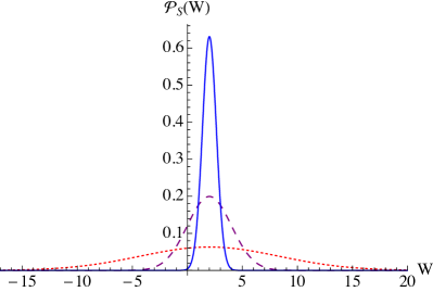
Figure 1: (color online) Quantum work density, $\mathcal{P}_{S}(W)$, for charged Schrödinger particles (17) with $A_{0}=0$, $A_{\tau}=1$, $m=1$, $c=1$, and $\beta=10$ (blue, solid line), $\beta=1$ (purple, dashed line), and $\beta=0.1$ (red, dotted line).

III.2 Dirac dynamics

In complete analogy to the preceding Schrödinger case we now compute the quantum work density for charged particles evolving under the time-dependent Dirac equation,

$$i\hbar\,\dot{\Psi}(p,t)=\left[\left(cp+A_{t}\right)\,\sigma_{x}+mc^{2}\,\sigma_{z}\right]\,\Psi(p,t)\,.$$ (18)

Equation (18) can be separated into two evolution equations for the components of the bispinor, $\Psi(p,t)=\left(\Psi_{1}(p,t),\Psi_{2}(p,t)\right)$, and we have

$$\begin{split}\hbar^{2}\,\ddot{\Psi}_{1}(p,t)&=-\left[(cp+A_{t})^{2}+\left(mc^{2}\right)^{2}+i\hbar\,\dot{A_{t}}\right]\,\Psi_{1}(p,t)\,,\\ \Psi_{2}(p,t)&=\left[i\hbar\,\dot{\Psi}_{1}(p,t)-(cp+A_{t})\Psi_{1}(p,t)\right]/mc^{2}\,.\end{split}$$ (19)

In contrast to the previous case (10) the solution of the time-dependent Dirac equation (18) is determined by an ordinary differential equation of second order (19). Therefore, to find analytical solutions of Eq. (18) we have to resort to particular parameterizations of $A_{t}$. For oscillating protocols Eq. (18) has been solved in Ref. Fillion-Gourdeau et al. (2012), and we will see two further examples in the following.

Before we turn to specific parameterizations, however, we note the instantaneous (positive) eigenenergies of Eq. (18),

$$\epsilon_{D}(\pi_{t},A_{t})=\sqrt{\left(c\pi_{t}+A_{t}\right)^{2}+\left(mc^{2}\right)^{2}}$$ (20)

and the corresponding, orthonormal eigenstates,

$$\Phi(p,\pi_{t})=\frac{\delta\left(p-(\pi_{t}+A_{t}/c)\right)}{\sqrt{1+\left(\sqrt{\Pi_{t}^{2}+1}-\Pi_{t}\right)^{2}}}\,\begin{pmatrix}1\\ \sqrt{\Pi_{t}^{2}+1}-\Pi_{t}\end{pmatrix},$$ (21)

where we introduced the notation $\Pi_{t}=(c\pi_{t}+A_{t})/mc^{2}$. One easily convinces oneself that these eigenstates, $\Phi(p,\pi_{t})$, fulfill the orthonormality condition (13).

For the following analysis we will assume that in the initial state, $\rho_{0}$, merely particles are present, but no antiparticles. This assumption is in full agreement with typical situations in nature and the mathematical treatment simplifies significantly . We emphasize that this assumption merely circumvents the conceptual issue of having to define a free energy for antiparticles. It has been shown that for any normalized initial state Deffner (2013) a fluctuation theorem can be derived. However, such a general theorem only reduces to a generalized Jarzynski equality for thermodynamically well-defined situations Deffner (2013). Nevertheless, for the sake of completeness, antiparticle energies and states can be found in Appendix A.

We also would like to emphasize that our analysis does not neglect the existence of antiparticles completely. We merely assume that the initial state is a thermal wave packet of particles. The dynamics, however, is described by the time-dependent Dirac equation (18), and hence governed by both, positive and negative eigenenergies. Hence, in particular the transition probabilities (4) are governed by both, particle and antiparticle solution.

Linear protocol

As a first example we consider a linearly parameterized vector potential,

$$A_{t}=\alpha\,t\,,$$ (22)

for which a solution of Eq. (19) is given by

$$\begin{split}\Psi_{1}(p,t)&=C_{1}(p)\,D_{-\nu}\left(\frac{(i+1)(cp+\alpha t)}{\sqrt{\alpha\hbar}}\right)\\ &+C_{2}(p)\,D_{\nu-1}\left(\frac{(i-1)(cp+\alpha t)}{\sqrt{\alpha\hbar}}\right)\,.\end{split}$$ (23)

Here, $D_{\nu}(\cdot)$ denotes the parabolic cylinder function Abramowitz and Stegun (1964) of order $\nu=i\,m^{2}c^{4}/2\alpha\hbar$, and $C_{1}(p)$ and $C_{2}(p)$ are time-independent functions of momentum determined by the initial state.

As mentioned earlier, for Dirac dynamics the solution is mathematically more involved, and also the amplitude of the wave function depends on the specific parameterization of $A_{t}$ – not only the phase as in the previous, non-relativistic case (14). This can be understood as dynamical interference of the two components of the bispinor. Nevertheless, the transition probabilities can still be written as

$$\mathfrak{p}_{D}\left(\pi_{0}\rightarrow\pi_{\tau}\right)=\left|\int\mathrm{d}p\,\Phi(p,\pi_{\tau})\cdot\Psi(p,t)\right|^{2}\,\mathfrak{p}_{0}^{D}(\pi_{0})\,,$$ (24)

where the initial distribution now reads

$$\mathfrak{p}_{0}^{D}(\pi_{0})=\exp{\left(-\beta\,\epsilon_{D}(\pi_{0},A_{0})\right)}/Z^{D}_{0}\,,$$ (25)

with which we can compute the quantum work distribution $\mathcal{P}_{D}(W)$ (3).

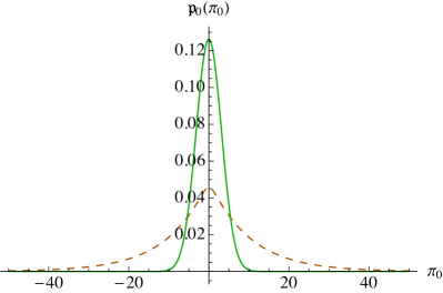
Figure 2: (color online) Thermal momentum distribution for Schrödinger (16) (green, solid line) and Dirac particles (25) (dark orange, dashed line) with $m=1$, $c=1$, $A_{0}=0$, and $\beta=0.1$.

In Fig. 2 we plot the thermal momentum distribution for Schrödinger particles (16) together with the distribution for Dirac particles (25). In the Schrödinger case we have the well-known (Gaussian) Maxwell-Boltzmann distribution. The momentum distribution for relativistic Dirac particles is broader due to the relativistic energy, $mc^{2}$, and was first described for classical mechanics by Jüttner Jüttner (1911). The so-called Maxwell-Jüttner distribution converges towards the Maxwell-Boltzmann distribution (16) for low temperatures, and decays slower than a Gaussian at high temperatures Jüttner (1911). The major limitation is that the Maxwell-Jüttner distribution neglects antiparticles, which however serves our present purpose.

The resulting work distribution, $\mathcal{P}_{D}(W)$, is plotted in Fig. 3, for the same parameters and color coding as for Schrödinger particles in Fig. 1.

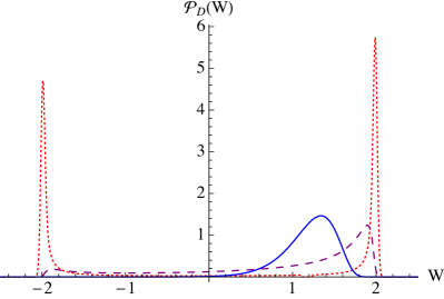
Figure 3: (color online) Quantum work density, $\mathcal{P}_{D}(W)$, for charged Dirac particles and the linear protocol (22) with $\alpha=1$, $\tau=1$, $\hbar=1$, $m=1$, $c=1$, and $\beta=10$ (blue, solid line), $\beta=1$ (purple, dashed line), and $\beta=0.1$ (red, dotted line).

As anticipated the relativistic effects change the characteristics of the quantum work distribution significantly. The most striking difference with the Schrödinger case in Fig. 1 is that $\mathcal{P}_{D}(W)$ has a finite support. This, however, can be understood intuitively: Large fluctuations in $W$ are accompanied by a large change in momentum. However, the momentum is limited by the light cone, and, hence, large fluctuations in $W$ are also “cut-off” by the light cone.

Quantitatively, the finite support can be determined by inspecting the transition probabilities (24). It is easy to see that $\mathfrak{p}_{D}\left(\pi_{0}\rightarrow\pi_{\tau}\right)\propto\delta\left(\pi_{0}-\left(\pi_{\tau}+A_{\tau}/c\right)\right)$. Hence, the only work values contributing to $\mathcal{P}_{D}(W)$ are $W=\epsilon_{D}(\pi_{0}+A_{\tau}/c,A_{\tau})-\epsilon_{D}(\pi_{0},A_{0})$, and therefore $W\in(-2\,\alpha\tau,\,2\,\alpha\tau)$.

Qualitatively, one can understand Fig. 3 by starting with the distribution for Schrödinger particles in Fig. 1, and “compressing” the curves into the allowed support. For low temperatures (blue curve) the left flank is rather unaffected, as the distribution lives “far away” from the light cone, whereas the right flank is only slightly deformed. For higher temperatures the effect becomes more prominent, and the distribution becomes “jammed” at the edges of the support, i.e., at the light cone.

Exponential protocol

To conclude the analysis we also compute the quantum work density (3) for a non-linear parameterization,

$$A_{t}=\alpha\left(1-\exp{\left(-t/\tau\right)}\right)\,.$$ (26)

Also in this case the time-dependent Dirac equation (19) can be solved analytically. However, the solution can no longer be written in compact form, and can be found in Appendix B. The transition probabilities (24) and the initial distribution remain the same by replacing Eq. (23) with the expression (31) everywhere.

Figure 4 illustrates the resulting quantum work distributions. We observe that the work distributions resulting from the linear protocol (22) and the exponential protocol (26) are nearly indistinguishable – despite the solutions (23) and (31) being complicated expressions of special functions. Thus, we conclude that the effect of the light cone on the work distribution is more prominent than the interference of the two components of the bispinor .

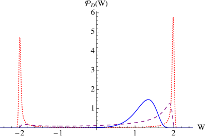
Figure 4: (color online) Quantum work density, $\mathcal{P}_{D}(W)$, for charged Dirac particles and the exponential protocol (26) with $\alpha=e/(e-1)$, $\tau=1$, $\hbar=1$, $m=1$, $c=1$, and $\beta=10$ (blue, solid line), $\beta=1$ (purple, dashed line), and $\beta=0.1$ (red, dotted line).

III.3 Jarzynski equality

The validity of the quantum Jarzynski equality follows from the unitarity of Dirac dynamics. Nevertheless, it is worthwhile to numerically verify its predictions. To this end, we numerically integrated the average exponentiated work for the distributions in Figs. 3 and 4. Here, the Jarzynski equality becomes,

$$\left\langle\exp{\left(-\beta W\right)}\right\rangle=\int\mathrm{d}W\,\mathcal{P}_{D}(W)\,\exp{\left(-\beta W\right)}=1\,,$$ (27)

as the free energy difference vanishes. In Table 1 we summarize the numerical results. We see that the quantum Jarzynski equality (27) is, indeed, verified to very high accuracy.

	$\beta=10$	$\beta=1$	$\beta=0.1$
linear	0.99	0.99	0.99
exponential	0.96	0.98	1.00

Table 1: Numerical verification of the quantum Jarzynski equality (27) for the quantum work distributions for Dirac particles in Figs. 3 and 4.

The validity of the quantum Jarzynski equality (27) explains another important feature of $\mathcal{P}_{D}(W)$. For the linear (22) as well as for the exponential (26) protocol left and right flank of the distribution are “exponentially asymmetric”. This asymmetry constitutes a necessary charactertistic of $\mathcal{P}_{D}(W)$ for Eq. (27) to hold. Note also that the asymmetry of $\mathcal{P}_{D}(W)$ is not an artifact of assuming that the initial state is comprised of only particles, but no antiparticles. We emphasize again that the existence of antiparticles is implicit in our treatment as the dynamics is described by Eq. (18).

IV Concluding remarks

In the present study we have analyzed the validity of the quantum Jarzynski equality and the properties of the quantum work distribution for systems described by the Dirac equation. For pedagogical reasons and for the sake of simplicity we focused on an illustrative case study. However, our system is more than a simple toy model, and it has realistic and experimental relevance.

IV.1 Experimental relevance

Only recently, Fillion-Gourdeau et al. Fillion-Gourdeau et al. (2012) studied the same model system in the context of pair production in counterpropagating laser light. However, Ref. Fillion-Gourdeau et al. (2012) not only solves Eq. (18) analytically for an oscillating parameterization of $A_{t}$, but also provides relevant values for the field strength, for which the dynamics could be observed in an experiment. It is worth emphasizing that Eq. (9) is only an approximate description of the real physical situation with a clearly defined range of validity Fillion-Gourdeau et al. (2012). Nevertheless, for all experiments for which Eq. (9) is valid our results could be readily verified, where one only would have to additionally measure the momentum distribution. From the momentum distribution one would compute the transition probabilities (24), and build the quantum work distribution (3) from a histogram. This procedure is fully analogous to the cold ion trap experiment, that verified the quantum Jarzynski equality Huber et al. (2008); An et al. (2015).

IV.2 Summary and outlook

Our present analysis has extended the scope of quantum stochastic thermodynamics to relativistic energies. We have shown that not only does the quantum Jarzynski equality hold for Dirac dynamics, but we also have provided a step-by-step “recipe” of how to compute the relativistic work distribution. For the sake of clarity and due to its mathematical simplicity we focused on free, charged particles traveling through a time-dependent vector potential. Another recent reference proposed to study pair production in a slightly more complicated, but also more realistic system including a scalar potential Fillion-Gourdeau et al. (2013). Our analysis could be straightforwardly applied to the situation of Ref. Fillion-Gourdeau et al. (2013) under the expense of having to compute $\mathcal{P}_{D}(W)$ fully numerically.

Appendix A Antiparticle energy and eigenstate

The instantaneous antiparticle solution of the time-dependent Dirac equation (18) is given by

$$\Phi^{a}(p,\pi_{t})=\frac{\delta\left(p-(\pi_{t}+A_{t}/c)\right)}{\sqrt{1+\left(\sqrt{\Pi_{t}^{2}+1}+\Pi_{t}\right)^{2}}}\,\begin{pmatrix}-1\\ \sqrt{\Pi_{t}^{2}+1}+\Pi_{t}\end{pmatrix}.$$ (28)

with eigenenergies

$$\epsilon_{D}^{a}(\pi_{t},A_{t})=-\sqrt{\left(c\pi_{t}+A_{t}\right)^{2}+\left(mc^{2}\right)^{2}}\,.$$ (29)

Note that the eigenenergies for antiparticles are negative. Thus, the Maxwell-Jüttner distribution (25) is ill-defined for positive temperatures.

Appendix B Analytical solution of time-dependent Dirac equation

For the exponential protocol,

$$A_{t}=\alpha\left(1-\exp{\left(-t/\tau\right)}\right)$$ (30)

a solution of the time-dependent Dirac equation (19) is given by

$$\begin{split}&\Psi_{1}(p,t)=\exp{\left(-\frac{i}{\hbar}\left(t\,\sqrt{(mc^{2})^{2}+(cp)^{2}+2pc\alpha+\alpha^{2}}+\alpha\tau\,e^{-t/\tau}\right)\right)}\\ &\times\bigg{[}C_{1}(p)\,U\left(-\frac{i\tau}{\hbar}\left(cp+\alpha-\tau\sqrt{(mc^{2})^{2}+(cp)^{2}+2cp\alpha+\alpha^{2}}\right),\,1+\frac{2i\,\tau}{\hbar}\sqrt{(mc^{2})^{2}+(cp)^{2}+2cp\alpha+\alpha^{2}},\,\frac{2i\,\alpha\tau}{\hbar}e^{-t/\tau}\right)\\ &+C_{2}(p)\,L\left(\frac{i\tau}{\hbar}\left(cp+\alpha-\tau\sqrt{(mc^{2})^{2}+(cp)^{2}+2cp\alpha+\alpha^{2}}\right),\frac{2i\,\tau}{\hbar}\sqrt{(mc^{2})^{2}+(cp)^{2}+2cp\alpha+\alpha^{2}},\,\frac{2i\,\alpha\tau}{\hbar}e^{-t/\tau}\right)\bigg{]}\,.\end{split}$$ (31)

Here, $U(\cdot,\cdot,\cdot)$ is the Kummer function, and $L(\cdot,\cdot,\cdot)$ denotes the Laguerre polynomial Abramowitz and Stegun (1964).

References

- Jarzynski (1997) C. Jarzynski, Phys. Rev. Lett. 78, 2690 (1997).
- Crooks (1999) G. Crooks, Phys. Rev. E 60, 2721 (1999).
- Ortiz de Zárate (2011) J. M. Ortiz de Zárate, Europhys. News 42, 14 (2011).
- Callen (1985) H. B. Callen, Thermodynamics and an Introduction to Thermostatistics (John Wiley Sons, New York City, NY, USA, 1985).
- Bustamante et al. (2005) C. J. Bustamante, J. Liphardt, and F. Ritort, Phys. Today 58, 43 (2005).
- Jarzynski (2015) C. Jarzynski, Nat. Phys. 11, 105 (2015).
- Jarzynski (2011) C. Jarzynski, Annu. Rev. Condens. Matter Phys. 2, 329 (2011).
- Liphardt et al. (2002) J. Liphardt, S. Dumont, S. B. Smith, I. Tinoco, and C. Bustamante, Science 296, 1832 (2002).
- Schuler et al. (2005) S. Schuler, T. Speck, C. Tietz, J. Wrachtrup, and U. Seifert, Phys. Rev. Lett. 94, 180602 (2005).
- Saira et al. (2012) O.-P. Saira, Y. Yoon, T. Tanttu, M. Möttönen, D. V. Averin, and J. P. Pekola, Phys. Rev. Lett. 109, 180601 (2012).
- Bérut et al. (2013) A. Bérut, A. Petrosyan, and S. Ciliberto, EPL (Europhysics Lett. 103, 60002 (2013).
- Tasaki (2000) H. Tasaki, (2000), arXiv:cond-mat/0009244 .
- Kurchan (2000) J. Kurchan, (2000), arXiv:cond-mat/0007360 .
- Talkner et al. (2007) P. Talkner, E. Lutz, and P. Hänggi, Phys. Rev. E 75, 50102 (2007).
- Campisi et al. (2011) M. Campisi, P. Hänggi, and P. Talkner, Rev. Mod. Phys. 83, 771 (2011).
- Hänggi and Talkner (2015) P. Hänggi and P. Talkner, Nat. Phys. 11, 108 (2015).
- Huber et al. (2008) G. Huber, F. Schmidt-Kaler, S. Deffner, and E. Lutz, Phys. Rev. Lett. 101, 070403 (2008).
- Dorner et al. (2013) R. Dorner, S. R. Clark, L. Heaney, R. Fazio, J. Goold, and V. Vedral, Phys. Rev. Lett. 110, 230601 (2013).
- Mazzola et al. (2013) L. Mazzola, G. De Chiara, and M. Paternostro, Phys. Rev. Lett. 110, 230602 (2013).
- Batalhão et al. (2014) T. B. Batalhão, A. M. Souza, L. Mazzola, R. Auccaise, R. S. Sarthour, I. S. Oliveira, J. Goold, G. De Chiara, M. Paternostro, and R. M. Serra, Phys. Rev. Lett. 113, 140601 (2014).
- An et al. (2015) S. An, J.-N. Zhang, M. Um, D. Lv, Y. Lu, J. Zhang, Z.-Q. Yin, H. T. Quan, and K. Kim, Nat. Phys. 11, 193 (2015).
- Abah et al. (2012) O. Abah, J. Roßnagel, G. Jacob, S. Deffner, F. Schmidt-Kaler, K. Singer, and E. Lutz, Phys. Rev. Lett. 109, 203006 (2012).
- Roßnagel et al. (2014) J. Roßnagel, O. Abah, F. Schmidt-Kaler, K. Singer, and E. Lutz, Phys. Rev. Lett. 112, 030602 (2014).
- Zhang et al. (2014) K. Zhang, F. Bariani, and P. Meystre, Phys. Rev. Lett. 112, 150602 (2014).
- Kafri and Deffner (2012) D. Kafri and S. Deffner, Phys. Rev. A 86, 044302 (2012).
- Prasanna Venkatesh et al. (2014) B. Prasanna Venkatesh, G. Watanabe, and P. Talkner, New J. Phys. 16, 015032 (2014).
- Watanabe et al. (2014) G. Watanabe, B. P. Venkatesh, and P. Talkner, Phys. Rev. E 89, 052116 (2014).
- Allahverdyan (2014) A. E. Allahverdyan, Phys. Rev. E 90, 032137 (2014).
- Roncaglia et al. (2014) A. J. Roncaglia, F. Cerisola, and J. P. Paz, Phys. Rev. Lett. 113, 250601 (2014).
- Manzano et al. (2015) G. Manzano, J. M. Horowitz, and J. M. R. Parrondo, (2015), arXiv:1505.04201 .
- Deffner and Saxena (2015) S. Deffner and A. Saxena, Phys. Rev. Lett. 114, 150601 (2015).
- Subasi and Hu (2012) Y. Subasi and B.-L. Hu, Phys. Rev. E 85, 11112 (2012).
- Horowitz (2012) J. M. Horowitz, Phys. Rev. E 85, 031110 (2012).
- Deffner (2013) S. Deffner, EPL (Europhysics Letters) 103, 30001 (2013).
- Campisi (2013) M. Campisi, New J. Phys. 15, 115008 (2013).
- Leggio et al. (2013a) B. Leggio, A. Napoli, A. Messina, and H.-P. Breuer, Phys. Rev. A 88, 042111 (2013a).
- Leggio et al. (2013b) B. Leggio, A. Napoli, H.-P. Breuer, and A. Messina, Phys. Rev. E 87, 032113 (2013b).
- Deffner and Lutz (2008) S. Deffner and E. Lutz, Phys. Rev. E 77, 021128 (2008).
- Talkner et al. (2008) P. Talkner, P. S. Burada, and P. Hänggi, Phys. Rev. E 78, 11115 (2008).
- Deffner et al. (2010) S. Deffner, O. Abah, and E. Lutz, Chem. Phys. 375, 200 (2010).
- Quan and Jarzynski (2012) H. T. Quan and C. Jarzynski, Phys. Rev. E 85, 031102 (2012).
- Silva (2008) A. Silva, Phys. Rev. Lett. 101, 120603 (2008).
- Smacchia and Silva (2013) P. Smacchia and A. Silva, Phys. Rev. E 88, 042109 (2013).
- Marino and Silva (2014) J. Marino and A. Silva, Phys. Rev. B 89, 024303 (2014).
- Fusco et al. (2014) L. Fusco, S. Pigeon, T. J. G. Apollaro, A. Xuereb, L. Mazzola, M. Campisi, A. Ferraro, M. Paternostro, and G. De Chiara, Phys. Rev. X 4, 031029 (2014).
- Mascarenhas et al. (2014) E. Mascarenhas, H. Bragança, R. Dorner, M. França Santos, V. Vedral, K. Modi, and J. Goold, Phys. Rev. E 89, 062103 (2014).
- Gong et al. (2014) Z. Gong, S. Deffner, and H. T. Quan, Phys. Rev. E 90, 062121 (2014).
- Leonard and Deffner (2015) A. Leonard and S. Deffner, Chem. Phys. 446, 18 (2015).
- Fingerle (2007) A. Fingerle, Comptes Rendus Phys. 8, 696 (2007).
- Albash et al. (2013) T. Albash, D. A. Lidar, M. Marvian, and P. Zanardi, Phys. Rev. E 88, 032146 (2013).
- Rastegin (2013) A. E. Rastegin, J. Stat. Mech. Theory Exp. 2013, P06016 (2013).
- Rastegin and Zyczkowski (2014) A. E. Rastegin and K. Zyczkowski, Phys. Rev. E 89, 012127 (2014).
- Nielsen and Chuang (2010) M. A. Nielsen and I. L. Chuang, Quantum computation and quantum information (Cambridge University Press, Cambridge, UK, 2010).
- Dirac (1928) P. A. M. Dirac, Proc. R. Soc. A 117, 778 (1928).
- Peskin and Schroeder (1995) M. E. Peskin and D. V. Schroeder, An Introduction To Quantum Field Theory (Frontiers in Physics) (Westview Press, Boulder, CO, USA, 1995).
- Fillion-Gourdeau et al. (2012) F. Fillion-Gourdeau, E. Lorin, and A. D. Bandrauk, Phys. Rev. A 86, 032118 (2012).
- Note (1) Antiparticles are characterized by their negative energies (28\@@italiccorr). Thus, the thermal distribution (25\@@italiccorr) would not be well-defined for positive temperatures. This conceptual issue appears to be sufficiently severe, that we decided to postpone the resolution of this problem to future work.
- Abramowitz and Stegun (1964) M. Abramowitz and I. A. Stegun, Handbook of mathematical functions with formulas, graphs, and mathematical tables (Washington D.C., USA, 1964).
- Jüttner (1911) F. Jüttner, Ann. Phys. 339, 856 (1911).
- Note (2) The indistinguishability of the work distributions for different protocols is a peculiarity of the very simple model. Thus it is reasonable to expect richer features for situations involving scalar potentials Fillion-Gourdeau et al. (2013) or space-dependent vector fields.
- Fillion-Gourdeau et al. (2013) F. Fillion-Gourdeau, E. Lorin, and A. D. Bandrauk, Phys. Rev. Lett. 110, 013002 (2013).