Clusters of galaxies in a Weyl geometric approach to gravity

Abstract

A model for the dark halos of galaxy clusters, based on the Weyl geometric scalar tensor theory of gravity (WST) with a MOND-like approximation, is proposed. It is uniquely determined by the baryonic mass distribution of hot gas and stars. A first heuristic check against empirical data for 19 clusters (2 of which are outliers), taken from the literature, shows encouraging results. Modulo a caveat resulting from different background theories (Einstein gravity plus $\Lambda CDM$ versus WST), the total mass for 14 of the outlier reduced ensemble of 17 clusters seems to be predicted correctly (in the sense of overlapping $1\,\sigma$ error intervals).

Introduction

This is a corrected, and in some lesser aspects improved, postprint version of the paper of the same title, published in Journal of Gravity (JG) volume 2016, article ID 9706704. The most important corrections refer to equs. (28) and (47) of the publication in JG. An error in JG (47) lead to a wrong relation between the acceleration due to the scale connection ($a_{\varphi}$) and the acceleration arising from the scalar field energy density ($a_{sf}$). The corrected form of JG (47) appears here as equ. (46) and has consequences for the model (equs. (50)ff.). It makes a new run of the data evaluation necessary, now based on the corrected dynamical equations. The new results are given in the updated tables 2, 3 and figs. 2 to 7. The overall picture of the empirical test does not change, although now three rather than two galaxy clusters agree with the model only in the $2\sigma$ range.

In this paper the gravitational dynamics of galaxy clusters is investigated from the point of view of Weyl geometric scalar tensor theory of gravity (WST) with a non-quadratic kinematic Lagrange term for the scalar field (3L) similar to the first relativistic MOND theory rAQUAL (“relativistic a-quadratic Lagrangian”) [24]. To make the paper as self-contained as possible, it starts with an outline of WST-3L (section 1). WST-3L has two (inhomogeneous) centrally symmetric static weak field approximations: (i) the Schwarzschild-de Sitter solution with its Newtonian approximation, which is valid if the scalar field and the WST-typical scale connection plays a negligible role; (ii) a MOND-like approximation which is appropriate under the constraints that the scale connection cannot be ignored but is still small enough to allow for a Newtonian weak field limit of the (generalized) Einstein equation. The acceleration in the MOND approximation consists of a Newton term and an additional acceleration of which three quarters are due to the energy density of the scalar field and one quarter to the scale connection typical for Weyl geometric gravity.

In centrally symmetric constellations the scalar field energy forms a halo about the baryonic mass concentrations. Besides the acceleration derived from the (Riemannian) Levi-Civita connection induced by the baryonic matter and the scalar field energy an additional acceleration component due to the Weyl geometric scale connection arises in the present approach. If the latter is expressed by a fictitious mass in Newtonian terms, a phantom halo can be ascribed to it. It indicates the amount of mass one has to assume in the framework of Newton dynamics to produce the the same amount of additional acceleration. The scalar field halo consists of true energy derived from the energy-momentum tensor; it is independent of the reference system, as long as one restricts the consideration to reference systems with low (non-relativistic) relative velocities. The phantom halo, on the other hand, is a symbolical construct and valid only in the chosen reference system (and scale gauge). For galaxy clusters we find two components of the scalar field halo, one deriving from the total baryonic mass in the MOND approximation of the barycentric rest system of the cluster (component 1), and one arising from the superposition of all the scalar field halos forming around each single galaxy in the MOND approximation of the latter’s rest system (component 2). Because velocities of the galaxies with regard to the cluster barycenter are small (non-relativistic) and also the energy densities are small, the two components can be superimposed additively (linear approximation). With regard to the barycentric rest system of the cluster a three component halo for clusters of galaxies arises, two components being due to the scalar field energy and one purely phantom (section 2).

The two component scalar field halo is a distinctive feature of the Weyl geometric scalar tensor approach; it is neither present in the non-relativistic MOND approaches nor in rAQUAL. One may pose the question whether it suffices for explaining the deviation of the cluster dynamics from the Newtonian expectation without additional dark matter. If we call the totality of the three components the transparent halo of the cluster (section 2.5), the question is whether the (theoretically derived) transparent halo can explain the dark halo of galaxy clusters, observationally determined in the framework of Einstein gravity and $\Lambda CDM$.

Section 3 contains a first test of the model by confronting it with empirical data on mass distribution available in the astronomical literature. A full-fledged test would presuppose an evaluation of raw observational data in the framework of the present approach and is beyond the scope of this study. Here we use recently published data on the total mass (dark plus baryonic), hot gas, and the star matter for 19 galaxy clusters, which have been determined from different observational data sources (and are thus more precise than earlier ones) [28], [26], [29]. 2 of the 19 clusters show a surprisingly large relation of total mass to gas mass. They are separated as outliers from the rest of the ensemble already by the authors of the study; so do we. 17 non-outlying clusters remain as our core reference ensemble.

In the mentioned studies total mass, gas mass and star mass are determined on the background of Einstein gravity plus $\Lambda CDM$. That raises the problem of compatibility with the WST framework. It is discussed in 3.1, 3.2 and leads to a certain caveat with regard to the empirical values for the total mass ($M_{200},\,M_{500}$) and the reference distances $r_{200},\,r_{500}$ to the cluster centers. But it does not seem to obstruct the possibility for a first empirical check of our model (section 3.2). More refined studies are welcome. They have to use the WST framework for evaluating the observational raw data or, at least, to analyze the transfer problem of mass data from one framework to the other in more detail.

For 14 of the 17 main reference clusters the empirical and the theoretical values for the total mass agree in the sense of overlapping $1\,\sigma$ error intervals. For the remaining three we find overlap in the $2\,\sigma$ range. The two outliers of the original study do not lead to overlapping intervals even in the $4\,\sigma$ range (section 3.6). In the present approach the dynamics of the Coma cluster is explained without assuming a component of particle dark matter. It is being discussed in more detail than the other clusters in section 3.5.

A short comparison with the halos of R. Sanders’ $\mu_{2}$-MOND model with an additional neutrino core [21], and with the NFW halo [14] is given for Coma (section 3.7). The paper is rounded off by a short remark on the bullet cluster (section 3.8) and a final discussion (section 4).

1 Theoretical framework

1.1 Weyl geometric scalar tensor theory of gravity (WST)

Among the family of scalar tensor theories of gravity the best known ones, and closest to Einstein gravity, are those with a Langrangian containing a modified Hilbert term coupled to a scalar field $\phi$. Their Lagrangian has the general form

$$L = \frac{1}{2}(\xi\phi)^{2}R+L_{\phi}-\frac{\lambda}{4}\phi^{4}\ldots$$ (1)

$$\mathfrak{L} = L\sqrt{|g|}\,,\qquad|g|=|det\,g|\,.$$

Here $g$ is an abbreviation for a 4-dimensional pseudo-Riemannian metric $g=(g_{\mu\nu})$ of signature $(-+++)$. $\phi$ is a real valued scalar field on spacetime, $L_{\phi}$ its kinetic term, $\xi$ a constant allowing for bridging the hierarchy between the Planck scale and cosmologically small quantities (like vacuum energy density), and the dots indicate matter and interaction terms. Under conformal rescaling of the metric,

$$g_{\mu\nu}\mapsto g^{\prime}_{\mu\nu}=\Omega^{2}\,g_{\mu\nu}\quad\mbox{ ($\Omega$ a positive real valued function), }$$ (2)

the scalar field changes with weight $-1$, i.e. $\phi\mapsto\phi^{\prime}=\Omega^{-1}\,\phi$. So far this is similar to the well known Jordan-Brans-Dicke (JBD) scalar-tensor theory of gravity [15], [8], [12], [11]. But here we work in a scalar-tensor theory in the framework of Weyl’s generalization of Riemannian geometry [3, 17, 18, 23, 24].

Crucial for the Weyl geometric scalar tensor approach (WST) is that the scalar curvature $R$ and all dynamical terms involving covariant derivatives are expressed in Weyl geometric scale covariant form. The Lagrangian density $\mathcal{L}$ is invariant under conformal rescaling for any value of the coefficient $\xi^{2}$ of the modified Hilbert term. For the matter and interaction terms of the standard model of elementary particles, scale invariance is naturally ensured by the coupling to the Higgs field which has the same rescaling behaviour as the gravitational scalar field. Although there is no complete identity, there is a close relationship between scale and conformal invariance in quantum field theory [16]. For classical matter we expect that a better understanding of the quantum to classical transition, e.g. by the decoherence approach, allows to consider scale invariant Lagrangian densities also. For the time being we introduce the scale invariance of matter terms in the Lagrangian as a postulate.

In our context an important consequence is the scale covariance of the Hilbert energy momentum tensor

$$T_{\mu\nu}=-\frac{2}{\sqrt{|g|}}\frac{\delta\mathcal{L}_{m}}{\delta g^{\mu\nu}}\,,$$ (3)

which is of weight $w(T_{\mu\nu})=-2$. That is consistent with dimensional considerations on a phenomenological level. It has been shown that the matter Lagrangian of quantum matter (Dirac field, Klein Gordon field) is consistent with test particle motion along geodesics (autoparallels) $\gamma(\tau)$ of the affine connection, if the underlying Weyl geometry is integrable (see below, equ. (8)) [3]. For classical matter we assume the same. It is to be expected that it can be proven similar to Einstein gravity.

We do not want to heap up too many technical details; more can be found in the literature given above. But we have to mention that a Weylian metric can be given by an equivalence class of pairs $(g,\varphi)$ consisting of a pseudo-Riemannian metric $g=g_{\mu\nu}dx^{\mu}dx^{\nu}$, the Riemannian component of the Weyl metric, and a differentiable one-form $\varphi=\varphi_{\mu}dx^{\mu}$, the scale connection (or, in Weyl’s original terminology, the “length connection”). $\varphi_{\mu}$ is often called the Weyl covector or even Weyl the vector field. In fact, $\varphi$ denotes a connection with values in the Lie algebra of the scale group $(R^{+},\cdot)$ and can locally be represented by a differentiable 1-form. The equivalence is given by rescaling the Riemannian component of the Weylian metric according to (2), while $\varphi$ has the peculiar gauge transformation behaviour of a connection, rather than that of an ordinary vector (or covector) field in a representation space of the scale group:

$$\varphi_{\mu}\mapsto\varphi^{\prime}_{\mu}=\varphi_{\mu}-\frac{\partial_{\mu}\Omega}{\Omega}\,$$ (4)

or, shorter, $\varphi^{\prime}=\varphi-d\log\Omega$.

A Weylian metric has a uniquely determined compatible affine connection $\Gamma$; in physical terms it characterizes the inertio-gravitational guiding field. It can be additively composed by the well known Levi-Civita connection ${}_{g}\Gamma$ of the Riemannian component $g$ of any gauge $(g,\varphi)$ and an additional expression ${}_{\varphi}\Gamma$ in the scale connection, in short

$$\Gamma=\,_{g}\Gamma+_{\varphi}\Gamma\quad\mbox{with}\quad{}_{\varphi}\Gamma^{\mu}_{\nu\lambda}=\delta^{\mu}_{\nu}\varphi_{\lambda}+\delta^{\mu}_{\lambda}\varphi_{\nu}-g_{\nu\lambda}\varphi^{\mu}.$$ (5)

Covariant derivatives $D$ in the Lagrangians (1), (below) (28), and consequently in the expression for the energy-momentum tensor of the scalar field (35, 36) below, denote those of Weyl geometry. For a covariant field $X^{\nu}$ of weight $w$ the derivativation $\nabla$ with regard to $\Gamma$ of (5) $D$ is supplemented by a term due to the scaling weight $w$ of $X$:

$$D_{\mu}X^{\nu}=\nabla_{\mu}X^{\nu}+w\,\varphi_{\mu}X^{\nu}=\partial_{\mu}X^{\nu}+\Gamma_{\mu\lambda}^{\nu}X^{\lambda}+w\,\varphi_{\mu}X^{\nu}.$$ (6)

It turns out that for the metric $g_{\mu\nu}$ the full covariant derivative is zero:

$$D_{\lambda}g_{\mu\nu}=0\quad\longleftrightarrow\nabla_{\lambda}g_{\mu\nu}+2\varphi_{\lambda}g_{\mu\nu}=0\,$$ (7)

This is the Weyl geometric compatibility condition between metric and affine connection (sometimes called “semi-metricity”).

In the low energy regime there are physical reasons to constrain the scale connection to the integrable case with a closed differentiable form $d\varphi=0$, i.e. $\partial_{\mu}\varphi_{\nu}=\partial_{\nu}\varphi_{\mu}$. Then $\varphi$ is a gradient (at least locally) and may be given by

$$\varphi_{\mu}=-\partial_{\mu}\omega\,.$$ (8)

This constraint is part of the defining properties of WST. Then it is possible to “integrate the scale connection away” [3]. Having done so, the Weylian metric, given as $(\tilde{g},\tilde{\varphi})$, is characterized by its Riemannian component $\tilde{g}_{\mu\nu}$ only (and a vanishing scale connection $\tilde{\varphi}_{\mu}=0$). By obvious reasons we call this the Riemann gauge. This is the analogue of the choice of Jordan frame in JBD theory.

In any case, the choice of a representative $g_{\mu\nu}$ also fixes $\varphi_{\mu}$; both together define a scale gauge of the Weylian metric. Conformal rescaling of the metric is accompanied by the gauge transformation of the scale connection (4). From a mathematical point of view all the scale gauges are on an equal footing, and the physical content of a WST model can be extracted, in principle, from any scale gauge. One only needs to form a proportion with the appropriate power of the scalar field.From the physical point of view there are, however, two particularly outstanding scale gauges. Of special importance besides Riemann gauge is the gauge in which the scalar field is scaled to a constant $\phi_{o}$ (scalar field gauge). For the particular choice of the constant value such that

$$(\xi\phi_{o})^{2}=(8\pi\,G)^{-1}=E_{pl}^{2}\,,$$ (9)

with the Newton gravitational constant $G$, this gauge is called Einstein gauge ($E_{pl}$ the reduced Planck energy). It is the analogue of Einstein frame in JBD theory. In this gauge the metrical quantities (scalar, vector or tensor components) of physical fields are directly expressed by the corresponding field or field component of the mathematical model (without the necessity of forming proportions).

In Riemann gauge $\Gamma$ reduces to ${}_{g}\Gamma$ by definition. Thus, in this gauge, the guiding field is given by the ordinary expression of the Levi-Civita connection. On the other hand, in Einstein gauge the measuring behaviour of clocks are most immediately represented by the metric field; and also other physical observables are most directly expressed by the field values in this scale. Then the expression of the gravitational field and with it the expressions for accelerations contain contributions from the Weylian scale connection. Thus a specific dynamical difference to Einstein gravity and Riemannian geometry (as well as to JBD theory) arises even in the case of WST with its integrable Weyl geometry.

Writing the scalar field $\tilde{\phi}$ in Riemann gauge $(\tilde{g},0)$ in exponential form, $\tilde{\phi}=e^{\omega}$, turns its exponent

$$\omega:=\ln{\tilde{\phi}}$$ (10)

into a scale invariant expression for the scalar field. In the following we shall omit the tilde sign to simplify notation. The scale connection $\varphi=\hat{\varphi}$ in scalar field gauge is then

$$\hat{\varphi}=-d\omega\,,$$ (11)

because $\Omega=\tilde{\phi}=e^{\omega}$ is the rescaling function from Riemann gauge to scalar field gauge. For more details see [2, 7, 17, 18, 24].

For the sake of consistency under rescaling we consider scale covariant geodesics $\gamma(\tau)$ with scale gauge dependent parametrizations of the geodesic curves of weight $w(\dot{\gamma})=-1$:

$$\dot{u}^{\lambda}+\Gamma_{\mu\nu}^{\lambda}u^{\mu}u^{\nu}-\varphi_{\mu}u^{\mu}u^{\lambda}=0\,,\qquad u^{\mu}=\dot{\gamma}^{\mu}\,$$ (12)

Here the affine connection contains a $\varphi$-dependent term in addition to the well-known Levi-Civita connection ${}_{\varphi}\Gamma^{\lambda}_{\mu\nu}$ derived from $g_{\mu\nu}$ (equ (5)). The last term on the l.h.s. of (12) takes care for the scale dependent parametrization (compare (6)). In this way we work with a projective family of paths.

For any gauge of the Weylian metric and the scalar field, $(g,\varphi,\phi)$, any timelike geodesic has thus a generalized proper time parametrization $\gamma(\tau)$ with $g_{\mu\nu}u^{\mu}u^{\nu}=-1$, where $u^{\mu}=\dot{\gamma}^{\mu}$. Inverting the coordinate time function $t(\tau)$ along the geodesic by $\tau(t)$ we have, in abbreviated notation, $\tau^{\prime}t^{\prime}=1$ and thus:

$$\frac{d^{2}x^{i}}{dt^{2}}=\frac{d\tau}{dt}\frac{d}{d\tau}(\frac{d\tau}{dt}\frac{dx^{i}}{d\tau})=\left(\frac{d\tau}{dt}\right)^{2}\frac{d^{2}x^{i}}{d\tau^{2}}-\left(\frac{dt}{d\tau}\right)^{-3}\frac{d^{2}t}{d\tau^{2}}\frac{dx^{i}}{d\tau}\,$$ (13)

With (equ. (12)) and indices $i,j,k=1,2,3$, $\mu,\nu\ldots=0,1,2,3$ this leads to

$$\frac{d^{2}x^{i}}{dt^{2}} = \left(\frac{d\tau}{dt}\right)^{2}\left(-\Gamma^{i}_{\mu\nu}\frac{dx^{\mu}}{d\tau}\frac{dx^{\nu}}{d\tau}+\varphi_{\mu}\frac{dx^{i}}{d\tau}\frac{dx^{\mu}}{d\tau}\right)$$

$$-\left(\frac{d\tau}{dt}\right)^{3}\frac{dx^{i}}{d\tau}\left(-\Gamma^{0}_{\mu\nu}\frac{dx^{\mu}}{d\tau}\frac{dx^{\nu}}{d\tau}+\varphi_{\mu}\frac{dt}{d\tau}\frac{dx^{\mu}}{d\tau}\right)$$

$$= -\Gamma^{i}_{\mu\nu}\frac{dx^{\mu}}{dt}\frac{dx^{\nu}}{dt}+\varphi_{\mu}\frac{dx^{i}}{dt}\frac{dx^{\mu}}{dt}+\Gamma^{0}_{\mu\nu}\frac{dx^{\mu}}{dt}\frac{dx^{\nu}}{dt}\frac{dx^{i}}{dt}-\varphi_{\mu}\frac{dx^{\mu}}{dt}\frac{dx^{i}}{dt}\,.$$

Happily, the length connection terms coming from the scale covariance modification of the geodesic equation (12) cancel. This is an expression of the fact that only the trace of the geodesic enters into the coordinate time parametrization of the dynamical equation (1.1). The equation of motion for mass points in Weyl geometric gravity, parametrized in coordinate time, becomes:

$$\frac{d^{2}x^{i}}{dt^{2}} = -\Gamma^{i}_{00}+\Gamma^{0}_{00}\frac{dx^{i}}{dt}-2\Gamma^{i}_{0j}\frac{dx^{j}}{dt}-\Gamma^{i}_{jk}\frac{dx^{j}}{dt}\frac{dx^{k}}{dt}$$

$$+2\Gamma^{0}_{0j}\frac{dx^{i}}{dt}\frac{dx^{j}}{dt}+\Gamma^{0}_{jk}\frac{dx^{i}}{dt}\frac{dx^{j}}{dt}\frac{dx^{k}}{dt}$$

In the result the dynamics of mass points in Weyl geometric gravity is governed by the guiding field (the affine connection), like in the semi-Riemannian case [25, equ. (9.1.2)]. Note, however, that in (1.1) the length connection enters into the affine connection and influences the dynamics because of (5).

The geodesic equation thus contains terms in the scale connection $\varphi_{\mu}$. In the low velocity, weak field regime the equation of motion reduces to the form well known from Einstein gravity $\frac{d^{2}x^{j}}{dt^{2}}=-\Gamma^{j}_{00}$. Here the $\Gamma^{j}_{00}=\,_{g}\Gamma^{j}_{00}+_{\varphi}\Gamma^{j}_{00}$ ($j=1,2,3$) are the coefficients of the Weyl geometric affine connection with ${}_{\varphi}\Gamma^{j}_{00}$ given by (5). This is the crucial modifying term for gravity in the Weyl geometric approach (low velocity case).

1.2 The weak field static approximation

We want to understand the scale connection for the motion of point particles. The free fall of test particles in Weyl geometric gravity follows scale covariant geodesics. It is governed by a differential equation formally identical to the one in Einstein gravity (1.1). Here we look at the weak field static case for low velocities in order to study the dynamics of stars in galaxies and galaxies in clusters. For studies of the gas dynamics and its modification in our framework the velocity dependent terms of (1.1) have to be taken into account. This is not being done here.

Analogous to Einstein gravity, the coordinate acceleration $a$ for a low velocity motion $x(\tau)$ in proper time parametrization is given by

$$a^{j}=\frac{d^{2}x^{j}}{d\tau^{2}}\approx-\Gamma^{j}_{oo}\,.$$ (16)

According to (5) the total acceleration decomposes into

$$a^{j}=-_{g}\Gamma^{j}_{oo}-_{\varphi}\Gamma^{j}_{\nu\lambda}=a^{j}_{R}+a^{j}_{\varphi}\,$$ (17)

($j=1,2,3$ indices of the spacelike coordinates), where

$$a^{j}_{R}=-_{g}\Gamma^{j}_{oo}$$ (18)

is the Riemannian component of the acceleration known from Einstein gravity. Clearly

$$a^{j}_{\varphi}=-_{\varphi}\Gamma^{j}_{oo}$$ (19)

represents an additional acceleration due to the Weylian scale connection. For a diagonal Riemannian metric $g=diag\,(g_{oo},\ldots,g_{33})$ the general expression (5) simplifies to $-_{\varphi}\Gamma^{j}_{oo}=-g_{oo}\varphi^{j}$. General considerations on observable quantities and consistency with Einstein gravity show that, in order to confront it with empirically measurable quantities, we have to take its expression in Einstein gauge if we want to avoid additional rescaling calculations [23, sec. 4.6].

For a (diagonalized) weak field approximation in Einstein gauge,

$$g_{\mu\nu}=\eta_{\mu\nu}+h_{\mu\nu},\qquad|h_{\mu\nu}|\ll 1\,,$$ (20)

with $\eta=\epsilon_{sig}\,\mbox{diag}(-1,+1,+1,+1)$, the Riemannian component of the acceleration is the same as in Einstein gravity. Its leading term (neglecting 2-nd order terms in $h$) is,

$$a^{j}_{R}=_{g}\Gamma^{j}_{oo}\;\approx\;\frac{1}{2}\eta^{jj}\partial_{j}h_{oo}\quad\mbox{(no summation over $j$)}\,.$$ (21)

In the limit, $\Phi_{N}:=-\frac{1}{2}h_{oo}$ behaves like a Newtonian potential

$$a_{R}\approx-\nabla\Phi_{N}\,,$$ (22)

where $\nabla$ is understood to operate in the 3 spacelike coordinate space with Euclidean coefficients as the leading term of the metric.

In Einstein gauge the Weylian scale connection $\hat{\varphi}_{\mu}$ arises from Riemann gauge by rescaling with $\Omega=e^{\omega}$, $\hat{\varphi}_{\mu}=-\partial_{\mu}\omega$ (4), and $a^{j}_{\varphi}\approx\varphi^{j}$. In other words, the additional acceleration due to the scale connection (19) is generated by the scale invariant representative $\omega$ of the scalar field as its potential:

$$a_{\varphi}\approx-\nabla\omega\,$$ (23)

If we compare with Newton gravity, we can calculate the fictitious mass density which one had to assume on the right hand side of the Poisson equation, in addition to the real masses, in order to generate the same amount of additional acceleration. Obviously here it is

$$\rho_{ph}=(4\pi G)^{-1}\,\nabla^{2}\omega\,.$$ (24)

In the terminology of the MOND literature the acceleration due to the Weylian scale connection corresponds to a phantom energy density $\rho_{ph}$. We see that already on the general level the dynamics of WST differs from Einstein gravity. Only for trivial scalar field, $\omega=const$, the usual Newton limit is recovered, otherwise it is modified. We shall explore how this modification relates to the usual MOND approaches.

1.3 WST gravity with cubic kinematic Lagrangian (WST-3L)

The most common form of the kinetic term for the scalar field is that of a Klein-Gordon field, $L_{\phi 2}=-\frac{\alpha}{2}D_{\nu}\phi D^{\nu}\phi$, quadratic in the norm of the (scale covariant) gradient. For our form of the gravitational Lagrangian (1) it is conformally coupled for $\alpha=-6\xi^{2}$. Inspired by the approach of the relativistic “a-quadratic Lagrangian” (rAQUAL), the first relativistic attempt of a MOND theory of gravity [5, 4], we find that a Weyl geometric scalar tensor theory of gravity leads to a MOND-like phenomenology if we add a cubic term to the kinetic Lagrangian of the scalar field

$$L_{\phi}=L_{\phi 2}+L_{\phi 3}\,.$$ (25)

The crucial difference to the early approach of rAQUAL is the scale covariant reformulation in the framework of Weyl geometry. It results in a different behaviour of the scalar field energy density. Bekenstein/Milgrom’s model relied crucially on implementing a transition function $f(y)$ between the Newton and the deep MOND regime into the kinetic term. The constraint of scale invariance of the Lagrangian reduces the underdetermination of the Lagrangian and suggests a slightly different form of the kinetic term. It is still quite near to the one of the relativistic AQUAL theory.

In the review paper [4] Bekenstein gives the rAQUAL Lagrangian in the form (his eq. (6))

$$L_{\psi}=-(8\pi G_{N})^{-1}L^{-2}f(L^{2}\,\partial_{\nu}\psi\,\partial^{\nu}\psi)\,,$$ (26)

where $L$ is “a constant with dimension of length introduced for dimensional consistency” (later it is identified as the MOND acceleration $a_{o}$ via $c^{2}\,L^{-1}=a_{o}$). Asymptotically $f(y)\sim\frac{2}{3}y^{\frac{3}{2}}$ for $y\ll 1$ (MOND regime); similarly $f(y)\sim y$ for $y\gg 1$ (Newton regime). $\psi$ is the logarithm of a rescaling function between the Jordan frame metric $\tilde{g}_{\mu\nu}$ (called the “physical” metric) and the Einstein frame (“primitive”) metric $g_{\mu\nu}$, $\tilde{g}_{\mu\nu}=e^{2\psi}g_{\mu\nu}$. Its role is very close to our $\omega$ in (10). A corresponding scale covariant form of the Lagrangian could be

$$L_{\phi 3}=(\xi\phi)^{2}(\xi^{-1}\phi)^{2}\,f((\xi^{-1}\phi)^{-2}\,\partial_{\nu}\omega\,\partial^{\nu}\omega)\,,$$ (27)

where in Einstein gauge $\xi^{-1}\phi_{o}$ plays the role of $a_{o}$ (up to a factor). The sign has deliberately been changed; the reasons are given below eq. (39).

We are here interested in additive modifications (19) of Einstein gravity, mainly in a domain in which the effects of the scale connection $\varphi_{\nu}=-\partial_{\nu}\omega$, compared with those of the Riemannian component of the metric, cannot be neglected. This will be called a regime with MOND approximation. For non-timelike $\nabla\omega$ the Lagrangian (27) becomes,

$$L_{\phi 3}=\frac{8}{3}\xi^{3}\phi^{-2}\,(D_{\nu}\phi\,D^{\nu}\phi)^{\frac{3}{2}}=(\xi\phi)^{2}(\frac{1}{4}\xi^{-1}\,\phi)^{-1}\,|\nabla\omega|^{3}\,,\qquad$$ (28)

where we have used the abbreviation

$$|\nabla\omega|:=\left|\partial_{\nu}\omega\,\partial^{\nu}\omega\right|^{\frac{1}{2}}$$ (29)

($|\dots|$ absolute value). $\omega$ is the scale invariant representative of the scalar field introduced in (10), and $\nabla$ its gradient.

With $\phi_{o}$ the (constant) value of $\phi$ in Einstein gauge we introduce the constants

$$a_{o}:=\xi^{-1}\phi_{o}\,,\qquad\tilde{a}_{o}=\frac{a_{o}}{4}\,.$$ (30)

Then the cubic term of the kinetic Lagrangian in Einstein gauge reads

$$L_{\phi 3}\doteq\frac{2}{3}(8\pi G\,\tilde{a}_{o})^{-1}|\nabla\omega|^{3}\,.$$ (31)

The dotted equality sign “$\doteq$”, indicates that the respective equation is not scale invariant but presupposes a special gauge made clear by the context (similar for $\dot{\approx}$). Here, as in most cases in this paper, it indicates the Einstein gauge. $\tilde{a}_{o}$ has the dimension of inverse length/time and will play a role analogous to the MOND acceleration $a_{o}\approx[c]\,H$ ($c$ the velocity of light). Coefficients of type $[c]$ and $[\hbar]$ will often be suppressed in the following general considerations. They will be plugged in only in the final step. The proportional factor in $\tilde{a}_{o}=\frac{a_{o}}{4}$ is chosen such that the WST model with cubic kinematic Lagrangian (WST-3L) acquires a MOND-like phenomenology in a weak gravitational field in which the scalar field and the scale connection cannot be neglected.

$\xi^{2}$ is a typical “large number” in the sense of bridging the gap between the smallest and the largest physically meaningful energy scales

$$\xi^{2}=\frac{E_{pl}}{a_{o}[\hbar]}=\frac{a_{o}^{-1}[c]}{L_{pl}}\sim 10^{63}\,.$$

To the kinetic Lagrangian of the scalar field a potential term is added. It must be of order 4 to provide for scale invariance of the density (eq. (1):

$$L_{V4}=-\frac{\tilde{\lambda}}{4}\phi^{4}$$ (32)

The absolute value of the corresponding energy density can be read off from

$$\frac{\tilde{\lambda}}{4}\phi^{4}=(\xi\phi)^{2}\,\frac{\tilde{\lambda}}{4}(\xi^{-1}\phi)^{2}\,;$$

in Einstein gauge it is constant. With $\lambda=\frac{\tilde{\lambda}}{36}$ it becomes

$$(\xi\phi)^{-2}|L_{V4}|=\frac{\tilde{\lambda}}{4}(\xi^{-1}\phi)^{2}\doteq\frac{\lambda}{4}\,36\,a_{o}^{2}\doteq\frac{\lambda}{4}H^{2}$$ (33)

comparable to the cosmological constant term $\Lambda=3\,\Omega_{\Lambda}\,H^{2}$ of the standard approach.

Variation of the Lagrangian leads to the dynamical equations of WST, the Einstein equation and the scalar field equation. The scale invariant Einstein equation is

$$Ric-\frac{R}{2}g=(\xi\phi)^{-2}T^{(m)}+\Theta\,,$$ (34)

where $g$ denotes the whole collection of metrical coefficients and $T^{(m)}$ the energy tensor of matter (3). The scalar field contributes to the total energy momentum with two terms, $\Theta=\Theta^{(I)}+\Theta^{(II)}$, the first of which is proportional to the metric (thus formally similar to a vacuum energy tensor):

$$\Theta^{(I)} = \phi^{-2}\left(-D_{\lambda}D^{\lambda}\phi^{2}+\xi^{-2}(L_{V4}+L_{\phi})\right)g\,$$ (35)

$$\Theta^{(II)}_{\mu\nu} = \phi^{-2}\left(D_{\mu}D_{\nu}\phi^{2}-2\xi^{-2}\frac{\partial L_{\phi}}{\partial g^{\mu\nu}}\right)\,\qquad$$ (36)

Varying with regard to $\phi$ gives the scalar field equation. Subtracting the trace of the Einstein equation for a conformally coupled $L_{\phi 2}$ term ($\alpha=-6\xi^{2}$) strongly simplifies it and introduces the trace of the matter tensor into the scalar field equation. In Einstein gauge, with $g$ the Riemannian component of the metric, it can be written in terms of the covariant derivative ${}_{g}\nabla$ with regard to $g$ (Levi-Civita connection in Einstein gauge) as

$$\,{}_{g}\nabla_{\nu}(|\nabla\omega|\partial^{\nu}\omega)\doteq-4\pi G\,\tilde{a}_{o}\,tr\,T^{(m)}\,.$$ (37)

If we introduce the corresponding Riemannian covariant operator

$${}_{g}\square_{M}\,\omega=\,_{g}\nabla_{\nu}(|\nabla\omega|\partial^{\nu}\omega)=\left(\partial_{\nu}|\nabla\omega|\,\partial^{\nu}\omega+|\nabla\omega|\,_{g}\nabla_{\nu}\,\partial^{\nu}\omega\right)\,,$$ (38)

the scalar field equation for a fluid with matter density $\rho_{m}$ and pressure $p_{m}$ simplifies to the covariant Milgrom equation

$${}_{g}\square_{M}\,\omega\doteq 4\pi G\,\tilde{a}_{o}\,(\rho_{m}-3p_{m})\,.$$ (39)

In this derivation, with $tr\,T^{(m)}$ entering by subtracting the trace of the Einstein equation, a sign choice like in (26) leads to the wrong sign on the r.h.s of the Milgrom equation. By obvious reasons (38) will be called the covariant Milgrom operator. In the static weak field static case $\omega$ does not depend on the time coordinate. Moreover with $g_{\mu\nu}\approx\eta_{\mu\nu}$, the expression $\nabla_{\nu}(|\nabla\omega|\partial^{\nu}\omega)$ turns into the nonlinear Laplace operator $\nabla\cdot(|\nabla\omega|\nabla\omega)$ of the MOND theory with Euclidean scalar product $\cdot$ and norm $|\ldots|$.

In the general case we have to complement (39) with the Einstein equation in Einstein gauge

$$Ric-\frac{R}{2}g\doteq 8\pi G\,T^{(m)}+\Theta\,,$$ (40)

In vacuum, the trivial scalar field $\omega=const$ is a basic solution of (39). Then WST reduces to Einstein gravity. In particular, the Schwarzschild and the Schwarzschild-de Sitter solutions of Einstein gravity are special (degenerate) solutions of WST-3L equations for $\frac{\lambda}{4}=0$ or $\frac{\lambda}{4}\approx 6$, respectively. In fact, they solve (40), (39) for $\phi\doteq const$ in Riemann gauge, i.e. in the case of Einstein gauge equal to Riemann gauge $(\hat{g},\hat{\varphi})=(\tilde{g},0)$. The Riemannian component of the metric ($\tilde{g}=\hat{g}=:g$) is given by

$$ds^{2}=-(1-\frac{2M}{r}-\kappa\,r^{2})dt^{2}+(1-\frac{2M}{r}-\kappa\,r^{2})^{-1}dr^{2}+r^{2}(dx_{2}^{2}+\sin^{2}x_{2}\,dx_{3})^{2}\,.$$ (41)

Then $Ric-\frac{R}{2}g=-3\kappa\,g$ and $\Theta=\Theta^{(I)}=-\frac{\lambda}{4}\beta^{2}\tilde{a_{o}}^{2}\,g$. Therefore the Einstein equation is satisfied for $3\kappa=\frac{\lambda}{4}\beta^{2}\,\tilde{a_{o}}^{2}$, i.e. $\kappa\approx 2H^{2}$ for $\frac{\lambda}{4}\approx 6$ and $\beta\approx 100$. We see that in the case of a negligible Weylian scale connection the classical (non-homogeneous) point-symmetric solutions of Einstein gravity are valid also for the dynamics of WST. This implies that in the case of a negligible scale connection Newton dynamics is an effective approximation for point symmetric solutions of WST (in Einstein gauge).

In order to make such a type of Einstein limit compatible with our Lagrangian, a suppression of the $L_{\phi 3}$-term for sufficiently large accelerations $a_{R}$ of (18) is necessary. Following the example of ordinary MOND theories, one might be tempted to plug a factor $\tilde{f}(\frac{a_{o}}{|a_{R}|})$ with a function $\tilde{f}$ such that $\tilde{f}(y)\sim 1$ for $y>0.01$ and $\tilde{f}(y)\sim 0$ for $y\ll 1$ into the r.h.s expression of (28) for $L_{\phi_{3}}$. But such a choice would have the blemish of a coordinate dependent argument of the function. A better alternative is provided by the hypothesis that the scalar field inhomogeneities are suppressed if any of the sectional curvatures $\kappa$ (with respect to the Riemannian component of the metric in Einstein gauge) surpasses a certain threshold, e.g., $\kappa\geq(10^{9}a_{o}[c^{-2}])^{2}$. In the next section we investigate the case of a non-negligible scale connection. A more detailed discussion of the transition between the two domains has to be left open for another occasion.

1.4 A WST approach with MOND-like phenomenology

If the conditions for the weak field approximation $(\ref{weak field})$ are given, it is possible to identify a MOND regime as a region in which the Newton acceleration $a_{N}$ is smaller than $a_{o}$ (here $a_{N}$ can be identified with $a_{R}$ in (22)). Then the scalar field equation (39) reduces, in reliable approximation, to

$$\nabla\cdot(|\nabla\omega|\nabla\omega)\doteq-4\pi G\,\tilde{a}_{o}\;tr\,T^{(m)}\,,$$ (42)

with the Euclidean $\nabla$-operator. We call this a MOND approximation. For pressure-less matter with energy density $\rho_{m}$ we get

$$\nabla\cdot(|\nabla\omega|\nabla\omega)\doteq 4\pi G\,\tilde{a}_{o}\,\rho_{m}\,.$$ (43)

That is similar to the AQUAL approach. Note that only the matter energy momentum tensor, without the scalar field energy density, appears on the r.h.s. of (42).

Straight forward verification shows that, independent of symmetry conditions, a solution of (43) is given by $\omega$ with a gradient $\nabla\omega=-a_{\varphi}$ such that

$$a_{\varphi}=\sqrt{\frac{\tilde{a}_{o}}{|a_{N}|}}\,a_{N}=\sqrt{\tilde{a}_{o}|a_{N}|}\,\frac{a_{N}}{|a_{N}|}\,,$$ (44)

where $a_{N}$ denotes the Newton acceleration of the given mass density,

$$\nabla^{2}\Phi_{N}=4\pi G\,\rho_{m}\,\qquad a_{N}=-\nabla\Phi_{N}$$ (45)

(calculations in the approximating Euclidean space with norm $|\ldots|$). The solution of the non-linear Poisson equation (43) is much simpler than one might expect at a first glance: In a first step the linear Poisson equation of the Newton theory is to be solved, then an algebraic transformation of type (44) leads to the acceleration due to the solution of the non-linear partial differential equation (43). In fact, $a_{\varphi}$ has the form of the deep MOND acceleration of the ordinary MOND theory (but with a different constant $\tilde{a}_{o}$).

This is only the most immediate modification of Newton gravity. In (40) there is also the additional term of the energy density due to the scalar field, $\rho_{sf}=(8\pi\,G)^{-1}\Theta_{oo}$. It modifies the r.h.s. of the Newton limit of Einstein gravity. Neglecting contributions at the order of magnitude of cosmological terms ($\sim H^{2}$) and of $|\nabla\omega|^{2}$), the energy density of the scalar field in Einstein gauge simplifies to

$$\rho_{sf}\;\dot{\approx}\;(4\pi G)^{-1}\nabla^{2}\omega\,,$$ (46)

where Latin indices $j,k$ …refer to space coordinates only (see appendix 5.1).

That is equal to the value of the phantom energy density corresponding to the acceleration of the scale connection (24). The total “anomalous” additive acceleration (in comparison to Newton gravity) is therefore

$$a_{add}=a_{\varphi}+a_{sf}=2a_{\varphi}\,.$$ (47)

In the central symmetric case

$$|a_{add}|=2\frac{\sqrt{GM(r)\,\tilde{a}_{o}}}{r}\,.$$ (48)

In the case of $a_{N}\ll a_{add}$ this leads to MOND-like phenomenology in the deep MOND regime if

$$\tilde{a}_{o}=\frac{a_{o}}{4}\approx\frac{1}{24}\,H\,[c]\approx 2.4\cdot 10^{-9}\,cm\,s^{-2}\,.$$ (49)

Because of (44) the total acceleration $a$ is then

$$a=a_{N}+a_{add}=a_{N}\left(1+\sqrt{\frac{a_{o}}{|a_{N}|}}\right)\,,\qquad|a_{add}|=\sqrt{a_{o}|a_{N}|}\,.$$ (50)

This raises the question of the Newtonian limit. (44) implies $|a_{\varphi}|\ll|a_{N}|$ in regions where $|a_{N}|\gg a_{o}\,(>\tilde{a}_{o})$. Therefore $a_{\varphi}$ can effectively be neglected in the case of ‘large’ values of $|a_{N}|$ derived from (45). Assuming the hypothesis at the end of section 1.3 (or some equivalent), the Newton approximation is reliable in WST gravity, irrespective of the question of how to characterize the transition between the MOND and the Newton approximation. Here we shall consider the MOND approximation in an “upper transition” regime only, where roughly $|a_{N}|\leq 10^{2}a_{o}$.

For centrally symmetric mass distributions $\rho(r)$ with mass $M(r)$ integrated up to $r$ (where $r=|y|$ denotes the Euclidean distance from the symmetry center, $y=(y_{1},y_{2},y_{3})$ the coordinates of the approximating Euclidean space) this implies

$$a_{\varphi}=-\nabla\omega\,\dot{\approx}-\sqrt{GM(r)\,\tilde{a}_{o}}\frac{y}{|y|^{2}}\,,\qquad|a_{\varphi}|=\frac{\sqrt{GM(r)\,\tilde{a}_{o}}}{r}\,.$$ (51)

Then the phantom energy density (24) becomes

$$\rho_{ph}=(4\pi G)^{-1}\frac{\sqrt{GM(r)\,\tilde{a}_{o}}}{r^{2}}\,;$$

and also

$$\rho_{sf}\;\dot{\approx}\;(4\pi G)^{-1}\frac{\sqrt{GM(r)\,\tilde{a}_{o}}}{r^{2}}\,.$$ (52)

1.5 Comparison with usual MOND theories

We can now compare our approach with other models of the MOND family. Simply adding a deep MOND term to the Newton acceleration of a point mass is unusual. M. Milgrom rather considered a multiplicative relation between the MOND acceleration $a$ and the Newton acceleration $a_{N}$ by a kind of ‘dielectric analogy’,

$$a_{N}=\mu(\frac{a}{a_{o}})\,a\;,\qquad\mbox{with}\quad\mu(x)\longrightarrow\left\{{1\quad\;\mbox{for}\;x\to\infty}\atop{x\quad\;\;\mbox{for}\;x\to 0\;,}\right.$$ (53)

or the other way round

$$a=\nu(\frac{a_{N}}{a_{o}})\,a_{N}\;,\qquad\mbox{with}\quad\nu(y)\longrightarrow\left\{{1\hskip 20.00003pt\mbox{for}\;y\to\infty}\atop{y^{-\frac{1}{2}}\;\;\mbox{for}\;y\to 0\;.}\right.$$ (54)

From this point of view our acceleration (50) is specified by a well defined transition functions

$$\mu_{w}(x)=1+\frac{1-\sqrt{1+4x}}{2x}\qquad\mbox{and}\quad\nu_{w}(y)=1+y^{-\frac{1}{2}}\;.$$ (55)

One has to keep in mind, however, that our transition functions $\mu,\nu$ are reliable only in the MOND regime and the upper transitional regime (roughly $a_{N}\leq 10^{2}a_{o}$). They cannot be used for discussing the Newtonian limit. It will be important to see how they behave in the light of empirical data, in particular galactic rotation curves and cluster dynamics.

In the MOND literature the amount of a (hypothetical) mass which in Newton dynamics would produce the same effects as the respective MOND correction $a_{add}$ is called phantom mass $M_{ph}$. For any member of the MOND family the additional acceleration can be expressed by the modified transition function $\tilde{\nu}=\nu-1$ with $\nu$ like in (54)

$$a_{add}=\tilde{\nu}\left(\frac{|a_{N}|}{a_{o}}\right)\,a_{N}\,.$$ (56)

The phantom mass density $\rho_{ph}$ attributed to the the potential $\Phi_{ph}$ satisfies $4\pi G\,\rho_{ph}=\nabla^{2}\Phi_{ph}$ and $\nabla\Phi_{ph}=-a_{add}$. A short calculation shows that it may be expressed as

$$\rho_{ph}=\tilde{\nu}\left(\frac{|a_{N}|}{a_{o}}\right)\,\rho_{m}-(4\pi G\,a_{o})^{-1}\tilde{\nu}^{\prime}\left(\frac{|a_{N}|}{a_{o}}\right)\,(\nabla|a_{N}|)\cdot a_{N}\,.$$ (57)

It consists of a contribution proportional to $\rho_{m}$ with factor $\tilde{\nu}$, which dominates in regions of ordinary matter, and a term derived from the gradient of $|a_{N}|$ dominating in the “vacuum” (where however scalar field energy is present). For the Weyl geometric model with $\tilde{\nu}_{w}(y)=y^{-\frac{1}{2}},\,\tilde{\nu}_{w}^{\prime}(y)=-\frac{1}{2}y^{-\frac{3}{2}}$ $\rho_{ph}$ turns into:

$$\rho_{t} = \left(\frac{a_{o}}{|a_{N}|}\right)^{\frac{1}{2}}\,\rho_{m}+(8\pi G)^{-1}\left(\frac{a_{o}}{|a_{N}|}\right)^{\frac{1}{2}}\,\nabla(|a_{N}|)\cdot\frac{a_{N}}{|a_{N}|}$$ (58)

$$\rho_{sf} = \rho_{ph}=\frac{1}{2}\rho_{t}\,$$ (59)

The first expression of (59) is compatible with (46).

In our case it would be utterly wrong to consider the whole of $\rho_{t}$ as “phantom energy”. Half of it are due to the scalar field energy density, the scalar field halo $\rho_{sf}$, and expresses a true energy density. This energy density appears on the right hand side of the Einstein equation (40) and the Newtonian Poisson equation as its weak field, static limit. It is decisive for lensing effects of the additional acceleration. The other half, $\rho_{ph}$, is phantom, i.e. a fictitious mass density producing the same acceleration as the Weylian scale connection (24). Only for the sake of comparison with other MOND models we may speak of $\rho_{t}$ as some kind of gross phantom energy,in contrast to the “net” phantom energy $\rho_{ph\,1}$.

We have to distinguish between the influence of the additional structure, scalar field and scale connection, on light rays and on (low velocity) trajectories of mass particles. Bending of light rays is influenced by the scalar field halo only, the acceleration of massive particles with velocities far below $c$ by the scalar field halo and the scale connection.

Also in another respect our theory differs from the usual MOND approaches. In MOND external acceleration fields of a system under consideration are difficult to handle. In WST, like in GR, a freely falling (small) system does not feel the external acceleration field if it is sufficiently small, relative to the inhomogeneities of the external gravitational field, for neglecting tidal forces. In this sense, the external acceleration problem does not arise in the WST MOND approximation (42).

Another important consequence follows: the scalar field energy formed around a freely falling subsystem of a larger gravitating system, calculated in the MOND approximation of the freely falling subsystem, contributes to the r.h.s. of the Einstein equation of any other subsystem (in relative motion) and also to that of a superordinate larger system. This has to be taken into account for modelling the dynamics of clusters of galaxies.

1.6 Short resumé

We have derived the most salient features of the Weyl geometric MOND approximation (WST MOND) and are prepared for a comparison with empirical data. Before we do so, it may be worthwhile to collect the results which are necessary for applying it to real constellations in a short survey.

Consider a gravitating system which in the Newton approximation of Einstein gravity is described by the baryonic matter density $\rho_{m}$, the acceleration $a_{m}$ and potential $\Phi_{m}$ with

$$\nabla^{2}\Phi_{m}=4\pi G\rho_{m}\,,\qquad a_{m}=-\nabla\Phi_{m}.$$ (60)

The modification due to WST MOND leads to an additional acceleration $a_{add}$ with the following features:

• The total acceleration $a$ is $a=a_{m}+a_{add}$ with

  $$a=a_{m}\left(1+\left(\frac{a_{o}}{|a_{m}|}\right)^{-\frac{1}{2}}\right)=\nu\left(\frac{|a_{m}|}{a_{o}}\right)a_{m}\,,$$ (61)

  where $\nu(y)=1+y^{-\frac{1}{2}}$. For $a_{m}\gg a_{o}$ the Newton approximation applies. (61) holds for $|a_{m}|\leq 10^{2}a_{o}$ only (“upper” transition regime). No information can be drawn from it for $|a_{m}|$ larger but not yet $\gg a_{o}$ (the “lower” transition regime).

• The “reciprocal” transformation function defined by $a_{m}=\mu\left(\frac{|a|}{|a_{m}|}\right)a$ is

  $$\mu(x)=1+\frac{1-\sqrt{1+4x}}{2x}\,.$$ (62)

• $a_{add}$ consists of two components $a_{add}=a_{\varphi}+a_{sf}=2a_{\varphi}$. The first one is derived from a potential $\omega$ satisfying the non-linear Poisson equation

  $$\nabla\cdot(|\nabla\omega|\nabla\omega)=\pi Ga_{o}\,\rho_{m}\,,\qquad a_{\varphi}=-\nabla\omega\,.$$ (63)

• The second one, $a_{sf}$, can be understood as a Newton acceleration due to the energy density $\rho_{sf}$ of a scalar field (part of the modified gravitational structure). Its potential satisfies a Newtonian Poisson equation. It satisfies

  $$-\nabla a_{sf}=4\pi G\rho_{sf}$$ (64)

  with energy density

  $$\rho_{sf}=\frac{1}{2}\left(\frac{a_{o}}{|a_{m}|}\right)^{\frac{1}{2}}\,\left(\rho_{m}+(8\pi G)^{-1}\nabla(|a_{m}|)\cdot\frac{a_{m}}{|a_{m}|}\right)$$ (65)

  $\rho_{sf}$ is part of the energy-momentum tensor of the scalar field $\phi$ and in this sense “real” rather than phantom.

• $a_{\varphi}$ is formally derivable in Newton dynamics from a fictitious energy density

  $$\rho_{ph}=\rho_{sf}\,.$$ (66)

  $\rho_{ph}$ is the net phantom energy of WST MOND. For comparison with other models of the MOND family one may like to consider $\rho_{ph}+\rho_{sf}=\rho_{t}$ as a kind of “gross phantom energy” (although the larger part of it is real). It is transparent rather than “dark” (see (74) below).

• (i) – (v) are reliable approximations also for small (local) gravitating systems freely falling in a larger gravitating system, if $a_{m}\lessapprox 10^{2}\,a_{o}$ in the local system. The subsystem can be considered as “small” with respect to the super-system, if tidal forces of the super-system can be neglected. In hierarchical systems like galaxy clusters the energy density contributions $\rho_{sf}$ of the subsystems and the super-system (calculated in different reference coordinate systems) add up to the total energy density of the scalar field, if the velocities of the subsystems relative to the barycenter of the super-system are small. This is a crucial difference between WST MOND and ordinary MOND theories. If one likes, $\rho_{sf}$ can be considered as the “dark matter” component of WST MOND; although as the energy density of the scalar field it is not constituted by the usual (hypothetical) quantum particles (WIMPs, axions etc.). To demarcate this difference it might better be called transparent matter/energy of WST.

• Gravitational lensing is due to the scalar field energy density only ($\rho_{sf}$), while the dynamics of WST corresponds to the total phantom density ($\rho_{t}=\rho_{sf}+\rho_{ph}$). It remains to be seen whether such a difference is in agreement with observations.

2 Halo model for clusters of galaxies

2.1 Cluster models for baryonic mass (hot gas and stars)

In the astronomical literature, the density profile of hot gas and (smeared) star/galaxy matter in a galaxy cluster is often described by a centrally symmetric profile of the following form:

$$\rho(r)=\rho_{o}\left(1+\left(\frac{r}{r_{c}}\right)^{2}\right)^{-\frac{3}{2}\beta}\,$$ (67)

$\beta$ is the ratio of the specific energies of the galaxies and the gas, $\rho_{o}$ the central density and $r_{c}$ is the core radius [20, 21, 19]. (67) is called a $\beta$-model for the mass distribution. For our test we assume density models for the gas mass $\rho_{gas}(r)$ and for the galaxy mass $\rho_{star}(r)$ with the same form parameters $\beta$ and $r_{c}$. We thus work with an idealized model using proportional density profiles for the hot gas and for the galaxies with parameters $\beta,r_{c}$ determined from observations of the hot gas. The central densities $\rho_{o}$ can, in principle, be determined from mass data for gas $M_{gas}(r_{1})$, respectively stars $M_{star}(r_{1})$, at a given distance $r_{1}$. The empirical determination of $M_{gas}(r_{1})$ and $M_{star}(r_{1})$ from directly observable quantities is a subtle question; it will be discussed in section 3.1.

Large scale gravitational effects on the cluster level are often modelled in the Newton approximation of Einstein gravity with baryonic matter and an assumed dark matter halo which is inferred from its gravitational effects (in Einstein/Newton gravity). Another, minority, approach in the literature works with an evaluation of the data in a MOND limit of the most well known relativistic MOND theory TeVeS. R. Sanders is one of its protagonists; he concludes that in this approach a much smaller amount of unseen matter has to be assumed in addition to the baryonic mass. Its value is consistent with the hypothesis of a halo of sterile neutrinos, concentrated about the cluster center [21]. Here we want to explore the feasibility of the WST approach, in particular regarding the question of how much unseen matter has to be added to the gravitational effects of the model in order to reproduce (“predict”) the observed accelerations, respectively their measurable effects.

2.2 Two contributions to the scalar field energy in clusters of galaxies

The mass distribution of the hot gas $\rho_{gas}$ in a galaxy cluster is described by a $\beta$-profile (67) in a locally static coordinate system with origin at the barycenter of the cluster. The averaged star mass will be represented by a continuous distribution $\rho_{star}$ of a $\beta$-profile with the same parameters $\beta,r_{c}$, but with a different value of $\rho_{o}$. Both together form a continuity model of the baryonic mass distribution $\rho_{bar}=\rho_{gas}+\rho_{star}$. Estimates show that Newtonian gravitational accelerations induced by $\rho_{bar}$ (far away from mass concentrations stars, galaxies, and galactic centers) are below $10^{2}\cdot a_{o}$. They are small enough for allowing to in a weak field static approximation with the scalar field equation in the MOND approximation (43). The resulting contribution to the scalar field energy will be called $\rho_{sf\,1}$. The additional acceleration of the Weyl geometrical scale connection (66) can be expressed in terms of a phantom mass density which will be called $\rho_{ph\,1}$.

In this first approximation the star mass is approximated on a par with the hot gas, i.e., it is described by its continuously smeared out mean density. But stars are agglomerated in galaxies which form freely falling subsystems of the cluster with considerable inter-spaces in the super-system (the cluster). For each subsystem a locally static coordinate system with origin at the respective galactic center can be chosen. In this system the local inhomogeneities of star mass distribution in the cluster, and the resulting inhomogeneities of the gravitational field, in the vicinity of of the galaxy can be calculated. On the galaxy level the MOND theory has proven effective for modelling gravitational effects deviating from Einstein and Newton gravity without assuming real dark matter [10]. Although we expect that the MOND approximation of WST gravity shows similar features, this is not the point in the present investigation.

Here we are interested in the neighbouring regions of galaxies as subsystems of their respective cluster. These subsystems form scalar field halos of their own which contain real energy (different from the classical MOND theory which leads to phantom halos only). In the framework of the present approach, the scalar field halos in the neighbourhood of each galaxy contribute to the energy density which adds up globally, i.e. on the cluster level, to a component of scalar field energy $\rho_{sf\,2}$ which has been suppressed in the first continuity approximation of the total baryonic mass. In a second step we therefore determine this component approximately and add it to the total the scalar field halo.

2.3 Scalar field and phantom halos $\rho_{sf\,1}$, $\rho_{ph\,1}$ in the cluster-barycentric MOND approximation

The baryonic mass up to radius $r$,

$$M_{bar}(r)=4\pi\int_{0}^{r}\rho_{bar}(u)\,u^{2}du\,,$$ (68)

determines the Newton acceleration $a_{bar}=G\frac{M(r)}{r^{2}}$ due to the total baryonic mass. The densities of the scalar field halo $\rho_{sf\,1}$ and the phantom halo of WST MOND follow from (65), (66). They are

$$\rho_{sf\,1} = \frac{1}{2}\left(\frac{a_{o}}{|a_{bar}|}\right)^{\frac{1}{2}}\,\left(\rho_{m}+(8\pi G)^{-1}\nabla(|a_{bar}|)\cdot\frac{a_{bar}}{|a_{bar}|}\right)\,,$$ (69)

$$\rho_{ph\,1} = \rho_{sf\,1}\,.$$ (70)

The respective masses of the halos $M_{sf\,1},\,M_{ph\,1}$ arise from integration.

2.4 Scalar field halos of galaxies in their respective galacto-centric MOND approximations

As already indicated in section 2.2 (69) and (70) do not make allowance for the fact that the star matter forms a discrete structure of an ensemble of galaxies each of which is falling freely in the inertio-gravitational field of the super-system (hot gas and other galaxies). Every galaxy possesses a local MOND approximation with regard to its own barycentric static reference system. The acceleration $a_{bar}$ of the super-system (with respect to the barycenter rest system of the hot gas) is transformed away in each of the local MOND approximations. The latter leads to a galactic scalar field halo which persists under changes of reference systems with small, i.e. non-relativistic, relative velocities. It contributes to the total energy of the scalar field, calculated in the cluster barycentric system. (Of course this is not the case for the phantom halo of the single galaxies.) In principle, we have to add up all these effects to a scalar field energy density $\rho_{sf\,2}$ in order to fill in this lacunae. But an exact calculation would have to solve a highly non-trivial $N$-body problem for the motion of the galaxies.

The experience with the calculation of the combined MOND halos of stars inside galaxies shows that a resolution of the star matter inside galaxies down to individual galaxies is not necessary to achieve good results. In the outer region of galaxies a continuity model for the distribution of star matter in the galactic disk gives reliable approximations for the MOND acceleration. Similarly we want to check whether also here a continuity model for the system of galaxies alone, abstracting from the gas mass, leads to an acceptable approximation for $\rho_{sf\,2}$. For this calculation, the gas mass has to be omitted because the galaxies are falling freely in the outer field of the cluster; the gravitational potential of the latter does not enter the local MOND approximation of the galaxies.

Using (65) again we get for the second (inhomogeneity) component of the scalar field energy

$$\rho_{sf\,2}=\frac{1}{2}\left(\frac{a_{o}}{|a_{star}|}\right)^{\frac{1}{2}}\,\left(\rho_{star}+(8\pi G)^{-1}\nabla(|a_{star}|)\cdot\frac{a_{star}}{|a_{star}|}\right)\,,$$ (71)

with $|a_{star}(r)|=G\frac{M_{star}(r)}{r^{2}}$ and $M_{star}(r)$ the integral analogous to (68) for the star density $\rho_{star}$.

We finally arrive at a halo model for galaxy clusters constituted by the components $\rho_{sf\,1},\rho_{sf\,2},\rho_{ph\,1}$. All of them are determined by the two component baryonic profile of the cluster.

2.5 A three-component halo model for clusters of galaxies

In addition to the Newtonian gravitational effects of the baryonic mass density

$$\rho_{bar}=\rho_{gas}+\rho_{star}\,,$$ (72)

modeled by a $\beta$-model of type (67), the WST MOND approach predicts accelerations generated by the scalar field halos (69), (71). Because of their small values their combined effect can be approximated by a linear superposition in the barycentric reference system of the cluster.

$$\rho_{sf}\approx\rho_{sf\,1}+\rho_{sf\,2}\,.$$ (73)

Moreover, there arises an acceleration $a_{\varphi}$ due to the scale connection in the barycentric rest system of the cluster (45). Its gravitational effects are representable by the fictitious (net) phantom halo $\rho_{ph\,1}$ of (70)

$$\rho_{ph\,1}=\rho_{sf\,1}\,.$$

On the other hand, the phantom energies of the individual freely falling galaxies do not survive the transformation to the cluster rest system and do not play a role on the cluster level.

In the usual MOND theories there is no scalar field energy; all additional effects with regard to Newton dynamics may be ascribed to a (fictitious) phantom energy density. Phantom energy densities of single galaxies do not survive the transformation to the cluster barycentric system. In MOND there is therefore no analogy to $\rho_{sf\,2}$; the latter is the crucial distinctive feature between the two approaches. For a comparison of WST-3L and usual MOND approaches with regard to galaxy clusters it is not sufficient to evaluate the difference between the transformation functions $\mu(x)$ (55).

For an even wider comparison with other approaches it may be useful to add up the scalar field and phantom halos to a kind of “dark matter” halo or, more precisely, to a substitute for the latter. But one must not forget that in the present model there is no dark matter in the ordinary sense. Here we only find a transparent halo made up of the (real) energy density of the scalar field and the (fictitious) phantom energy density ascribed to the acceleration effects of the scale connection in Einstein gauge (with respect to the cluster barycentric rest system):

$$\rho_{t}=\rho_{sf}+\rho_{ph\,1}\,$$ (74)

From the gravitational lensing point of view, it would be even more appropriate to consider $\rho_{sf}$ alone as the WST equivalent of a dark matter halo, not forgetting that even the real halo $\rho_{sf}$ is not due to fermionic particles, but to the scalar field, and thus to the extended gravitational structure of WST. From a quantum point of view, the scalar field has to be quantized if one wants to search for a (bosonic) particle content of $\rho_{t}$ or $\rho_{sf}$.

The total dynamical mass of the model (up to some distance $r$ from the center of the cluster) is

$$M_{tot}=M_{bar}+M_{t},\quad M_{t}=M_{sf}+M_{ph\,1},\quad M_{sf}=M_{sf\,1}+M_{sf\,2}\,$$ (75)

with $M_{bar}=M_{gas}+M_{star}$. The lensing mass is a bit smaller,

$$M_{lens}=M_{bar}+M_{sf}\,.$$ (76)

Mathematically, the integral of the scalar field energy density to arbitrary distances diverges. Like in the dark matter approach a virial radius of a cluster may be defined, which roughly delimits the gravitational binding zone of the cluster. Comparing $\rho_{t}$ (respectively ($\rho_{sf}$)) with the critical energy density $\rho_{crit}$ of the universe, one may, for example choose $r_{200}$ with

$$\rho_{t}(r_{200})\approx 200\,\rho_{crit}$$ (77)

as a representative of the virial radius.

Not far beyond the gravitational binding zone of the cluster, the energy density will have fallen to such a small amount that its centrally symmetric component is inconceivably stronger than the density fluctuations in the inter-cluster space. To continue the integration into this region, and beyond, has no physical meaning. In the long range the energy density of the scalar field approaches the cosmic mean energy value. A physical limit of integration has to be chosen close to the virial radius beyond which the gravitational binding structure of the cluster is fading out.

3 A first comparison with empirical data

3.1 Empirical determination of mass data for galaxy clusters

For a first empirical exploration we confront the WST cluster model with recent mass data for 19 clusters obtained on the background of Einstein/Newton gravity and $\Lambda$CDM by a group of astronomers about Y.-Y. Zhang, T.F. Laganá and T. Reiprich [28], [29]. We use the form parameters $\beta,r_{c}$ of the $\beta$-models of these clusters, published in an earlier study by one author of the group [19]. In the present study we have to take the mass data and the form parameters essentially at face value. Methodological questions arising from this procedure are discussed in the next subsection. There seem to be sufficient reasons for expecting that the different background theories do not principally invalidate the results thus obtained. Of course, an authoritative empirical study would presuppose an evaluation of observational data on the background of WST itself; it can be done only by astronomers, if they get interested in the present approach.

The studies of Zhang/Laganá/Reiprich e.a. have the great advantage to build upon three independent observational data sets for determining the gas mass $M_{gas,500}$, the star mass $M_{\ast,500}$ and the total mass $M_{500}$ (assuming a dark matter explanation for the observed gravitational effects) at the reference distance $r_{500}$. The latter is determined for each cluster at the distance $r_{500}$ from the cluster center at which the total gravitational acceleration indicates a total mass density 500 times the critical density.

• $M_{gas,500}$ has been extracted from X-ray data on the hot intracluster medium (ICM) collected by XMM Newton and ROSAT. Surface brightness data have been used to infer an ICM radial electron number density profile, and spectral analysis data gave information on the radial temperature distribution. From that a gas density distribution has been reconstructed and the gas masses at $r_{500}$ by integration.

• $M_{\ast,500}$ has been determined from optical imaging data due to SDSS 7 in two steps. First the total luminosity of the cluster has been determined by means of a “galaxy luminosity function” (GLF); then the mass is estimated using mass-to-light ratios depending on the cluster mass. In the last step models of the star development in the respective galaxy, elliptical or spiral, enter. They depend on assumptions on an “initial mass function” (IMF). Two possibilities for the IMF (Salpeter versus Kroupa) are considered and compared in [28], [29]. According to the authors the difference of the stellar mass estimate can result in a factor 2 [28, p.4 ].

• The total cluster mass $M_{500}$ has been determined on the basis of the velocity dispersion of galaxies, using spectroscopic data from [27, tab. 1]. The mass estimator used is eq. (2) of [6]

  $$M_{v}=A(\frac{\sigma_{v}}{10^{3}\,kms^{-1}})^{3}\times 10^{14}h^{-1}\,M_{\astrosun}\,,$$ (78)

  $A=1.50\pm 0.02$, $\sigma_{v}$ the 3-dimensional velocity dispersion inside a sphere of virial radius (by convention $r_{v}=r_{200}$). Reasons for this choice are given in [6, sec. 3]. $M_{500}$ was then determined from $M_{200}$ by a NFW-model.

3.2 Theory dependence of mass data for galaxy clusters

Mass densities of the hot gas and of star matter in galaxy clusters are indirectly inferred from observable quantities; they are thus theory dependent. Even inside the same background theory they may depend on choices of models and methods of evaluation.

That makes it a difficult task to compare our model with empirical data. A fine-grained judgement presupposes an evaluation of observational raw data on the background of WST gravity or, at least, a detailed estimation of systematic errors resulting from a comparison of different background theories (Einstein gravity with $\Lambda CDM$ and Newton approximation, or alternatively TeVeS-MOND, in comparison with WST and its MOND approximation). This task has to be left to astronomers, if they become sufficiently interested in the present approach. But, taking this caveat in mind, it still seems possible to confront available data from, e.g., the Einstein gravity-$\Lambda CDM$-Newton approximation framework with our model, in order to get a first impression of its potential usefulness. A comparison with mass data derived in a TeVeS-MOND background would give welcome supplementary information. This is not attempted here.

Let us discuss the possibility and the problems of a confrontation of these data with the MOND-approximation of WST:

• The mass of the hot gas (intracluster medium) $M_{gas\,500}$ (at $r_{500}$) has been determined in the mentioned study from X-ray data obtained by XMM-Newton and ROSAT. The temperature of the gas is estimated by a fit to the measured spectrum. The gas density $\rho(r)$ is reconstructed, using model assumptions, from intensity observables and then integrated up to $r_{500}$. Up to usual model dependence, the transfer of the mass data from the standard gravity background to WST seems to be relatively uncritical.

• Several methods for determining the stellar mass $M_{\ast\,500}$ are mentioned in [29]. In this study the star mass is gained from optical imaging data due to SDSS 7 in two steps indicated in (ii) above. According to the authors the difference of the stellar mass estimate due to different initial mass functions can result in a factor 2 [28, p.4 ]. Another approach would be to estimate stellar masses of the individual galaxies and “to construct the stellar mass functions in order to sum the stellar masses” (ibid, 1). Moreover, an additional component of star matter can be associated to the intracluster light. All in all, the estimate of the star mass concentrated in galaxies seems to depend more on models of galactic star evolution than on the background gravity theory. In spite of that the precision cannot be expected to be better than by a factor 2 (respectively 0.5).

• In Einstein gravity/$\Lambda CDM$ the cluster mass can, in principle, be estimated from the velocity dispersion $\sigma$ of galaxies at distance $R$ (from the center) by an estimator derived from the virial theorem $M\approx G^{-1}\sigma^{2}R$. The additional acceleration of WST-3L $a_{add}=a_{\varphi}+a_{sf}$ (47) is dynamically indistinguishable from the effects of “true” Newtonian masses. So far it seems as if the estimation of total mass can be transferred to the MOND approximation of WST without problems. But if the radius $R$ does not include the “whole” cluster mass (however defined), as is here the case (item (iii) last subsection) a surface pressure term must be taken into account. That complicates the case.

  In standard gravity the necessary correction is implemented by a cubic mass estimator $M\sim\sigma^{3}$ given above as (78). Moroever, the authors of our reference study [28] reconstruct $M_{500}$ and $r_{500}$ from these values using the NFW profile. Because of the different profile for the scalar field halo of WST this is a critical step for our exercise. On the other hand, if the resulting systematic errors are smaller than the error intervals of $M_{tot}$ (75), implied by the observational errors of the other quantities, they do not disturb a rough empirical check of the model.

• Finally the dependency of the data evaluation on the background cosmology has to be taken into account. The data of the 19 clusters used in the following have redshift $z<0.1$. The geometrical and dynamical corrections implied by the $\Lambda CDM$ cosmology are correspondingly small. An evaluation in, e.g., a Lemaitre-de Sitter model (or even a non-expanding Weyl geometric model with redshift) [24, section 4.2] would affect the data only by a minor expansion of the error intervals.

The points (1), (2) and (4), in particular the estimate of stellar mass concentrated in galaxies and gas mass, are fairly insensitive against a change of the background theory from Einstein gravity to WST. The theory dependence of $r_{500}$ is uncritical in our context. Any other reference radius could have been taken, as long as it is specified in astronomical distance units. The estimate for the total masses at $r_{500}$ and $r_{200}$ is the critical point for our purpose (item (3)). However, if the difference of the halo profiles between the scalar field energy density of WST and NFW dark matter does not push the estimates for the total masses $M_{500},\,M_{200}$ outside the error intervals of our halo model (due to observational input data), we may still be able to draw first inferences from the following evaluation.

3.3 Empirical data for 19 clusters

The studies [28], [29] contain new data on the baryon content and the total gravitational mass for 19 clusters of galaxies (as it appears in an Einstein–$\Lambda CDM$ framework with Newton approximation). The mass data $M_{500},M_{gas\,500},M_{\ast\,500}$ are given in columns (5), (7), (8) of table 1 in [29]. It is reproduced in our fig. 1. The values for $r_{500}$ are published in [26, tab. 1, col. (5)] (here table 1). A comparison of the total cluster masses derived from the velocity dispersion with a mass estimate derived from the gas mass shows that the two clusters A2029 and A2065 are outliers, with total cluster masses considerably higher than the corresponding gas masses would let expect. The authors therefore separate the two outliers from the rest of the data, with the remaining 17 clusters as a reliable data set [28, p. 3]. We shall do the same.

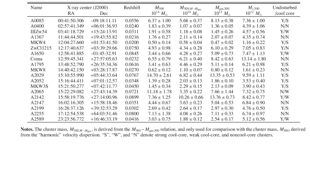
Figure 1: Tab.1 of [29]. Properties of the 19 galaxy clusters

Parameters ($\beta,\,r_{c}$) for the models of these galaxy clusters (as well as of many more) have been published earlier in [19, tab. 4.1]. This publication also contains mass data $M_{200},\,M_{gas\,200}$ at $r_{200}$ (with error intervals), mass values $M_{A},\,M_{gas\,A}$ (without error interval) at the Abell radius, here defined as $r_{A}=2.14\,Mpc$, but no data for star masses. In [19] the methods for determining the total mass and the gas mass were not yet as refined as in the later study. It is therefore not possible to aggregate the different data sets to one coherent ensemble. As no updated values for the parameters ($\beta,\,r_{c}$) of the mass profiles were available to the present author, the values of [19] are here used as estimators for the form parameters of the $\beta$ model.

We consider $M_{500},\,M_{gas\,500},\,M_{\ast\,500},$ $r_{500}$ from [28, 29] as our crucial mass data (including reference radii). Mass data at $r_{200}$ (as well as $r_{200}$ itself) from the older study are welcome as additional information; but they will not be used as core criteria for the empirical test of our model. Table 1 collects the data used. It shows that the cluster ensemble covers an order of magnitude variation for the gas mass $M_{gas\,500}$ and one and a half orders of magnitude variation in total mass $M_{500}$. The selection method by intersecting the cluster sets of different raw data sources does not seem to be influenced by any particular bias. We thus may consider the collection as a reasonable data set for testing our cluster halo model.

Table 1. Data set used for halo model (error intervals omitted)
Cluster $\beta$ $r_{c}$ $r_{500}$ $M_{500}$ $M_{gas\,500}$ $M_{\ast\,500}$ $M_{200}$ $r_{200}$ $M_{A}$ Coma 0.654 246 1.278 6.55 8.42 13.14 13.84 2.3 12.86 A85 0.532 59.3 1.216 6.37 8.13 7.36 7.71 1.9 8.72 A400 0.534 110. 0.712 1.83 1.36 4.39 1.48 1.09 2.93 IIIZw54 0.887 206 0.731 1.91 1.45 4.57 2.81 1.35 4.51 A1367 0.695 274 0.893 1.76 2.07 4.35 4.06 1.53 5.77 MKW4 0.44 7.86 0.58 0.5 0.47 1.16 0.71 0.86 1.79 ZwCl215 0.819 308 1.098 4.93 6.1 7.05 10.37 2.09 10.65 A1650 0.704 201 1.087 3.44 5.09 7.47 11.14 2.15 11.11 A1795 0.596 55.7 1.118 3.41 5.11 6.21 10.99 2.14 11.04 MKW8 0.511 76.4 0.715 0.62 0.8 1.61 2.38 1.28 4.0 A2029 0.582 59.3 1.275 14.7 13.35 9.59 13.42 2.29 12.59 A2052 0.526 26.4 0.875 1.39 1.86 3.53 2.21 1.25 3.79 MKW3S 0.581 47 0.905 1.45 2.13 3.9 3.46 1.45 5.11 A2065 1.162 493 1.008 11.18 7.66 7.32 16.69 2.45 14.46 A2142 0.591 110 1.449 7.36 13.76 8.42 15.03 2.36 13.61 A2147 0.444 170. 1.064 4.44 5.04 6.84 3.46 1.45 5.15 A2199 0.655 99.2 0.957 2.69 2.97 4.76 4.80 1.62 6.37 A2255 0.797 423 1.072 7.13 7.11 6.74 13.32 2.27 12.52 A2589 0.596 84.3 0.848 3.03 2.54 5.12 3.58 1.47 5.24
Source: first and last block [19], middle block [29], $r_{500}$ [26]
Units: $r_{c}$ in $kpc$, $r_{500},r_{200}$ in $Mpc$, $M_{500}$ in $10^{14}$ $M_{\astrosun}$, $M_{gas\,500}$ in $10^{13}$ $M_{\astrosun}$, $M_{\ast\,500}$ in $10^{12}$ $M_{\astrosun}$,

3.4 Adapting the WST halo model to the data

For the construction of the model we have to work in Einstein gauge (9). Consistency with the deep MOND acceleration demands (49). Taken together these conditions fix the coefficients of the Lagrangian (1) and (28), independently of the convention chosen for $\phi_{o}$. With a value for $\lambda$ on the order of magnitude 10 (e.g., $\frac{\lambda}{4}=6$ like at the end of section 1.3) the contribution of the $L_{V4}$ term lies many orders of magnitude below the energy densities the dominant term in (35) and is negligible in our context.

In agreement with section 2 the test of our halo model for each of the 19 galaxy clusters can now proceed as follows:

• Specification of the $\beta$ models (67) for gas and for star mass; parameters ($\beta,\,r_{c}$) from [19], $\rho_{o}$ determined by fitting to $M_{gas\,500}$ and $M_{\ast\,500}$ at $r_{500}$ respectively [29].

• Determination of the Newton accelerations of the baryonic mass components.

• Calculation of the scalar field halo and the phantom halo of the baryonic mass by (69), (66).

• Calculation of the scalar field halo of the system of freely falling galaxies (71).

• Aggregation of these to the total halo (74); choice of fading out functions beyond $r_{200}$ (see appendix).

• Integration of the densitities to the corresponding masses: scalar field energy of the galaxies $M_{sf\,2}$, of the gas mass $M_{sf\,1}$, total scalar field halo $M_{sf}$, net phantom energy of the baryonic mass $M_{ph\,1}$, finally the total transparent matter $M_{t}$ and the lensing mass $M_{lens}$ (75), (76).

• Calculation of the error intervals of the model at selected distances ($r_{500},\,r_{200}$).

• Comparison of the empirical value for $M_{500}$ (respectively $M_{200}$) with the model value $M_{t}(r_{500})$ (resp. $M_{t}(r_{200})$).

The result of this test are given in subsection 3.6. Before we turn to the overall evaluation, we shall have a look at one cluster as an exemplary case.

3.5 The WST halo model with the Coma cluster as test case

For a first check of our model we choose the Coma cluster. According to item (1) of the last section we use the empirical input data from table 1 (units given there):

$$(\beta,r_{c},r_{500},M_{gas\,500},M_{\ast\,500})=(0.654,\,246,\,1.278,\,8.42,\,13.14)\,,$$ (79)

($r_{c}$ in $kpc$, $r_{500}$ in $Mpc$, $M_{gas\,500}$ in $10^{13}M_{\astrosun}$, $M_{\ast\,500}$ in $10^{12}M_{\astrosun}$). The different components of the cluster halo integrate to masses (up to distance $r$) documented in fig. 2.

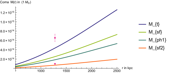
Figure 2: Halo components of Coma cluster: transparent matter halo $M_{t}=M_{sf}+M_{ph\,1}$, total scalar field (SF) halo $M_{sf}$, halo of freely falling galaxies $M_{sf\,2}$, and net phantom energy $M_{ph\,1}$ (in barycentric rest system).
Empirical data (violet dot and bar): baryonic mass $M_{\ast\,500}+M_{gas\,500}$ (dot) and $M_{500}$ (with error intervals) at $r_{500}=1280\,kpc$.

The scalar field halo (SF) of the total baryonic mass $\rho_{sf\,1}$ contributes the lion share to the total transparent energy. The SF of the galaxy system $\rho_{sf\,2}$ carries about as much energy as the net phantom component $\rho_{ph\,1}$ in the barycentric rest system of the cluster. It surpasses the gas mass close to the reference radius $r_{500}$. Figure 3 shows the fast increase of the gravitational mass of the scalar field halo of the galactic system.

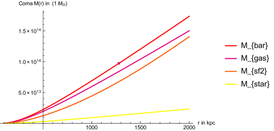
Figure 3: Comparison of the contribution of the scalar field halo of the galaxies $M_{sf2}$ with the baryonic mass for the Coma cluster (empirical data for $M_{bar\,500}$ violet dot).

If we add all baryonic and halo contributions, the picture given in fig. 4 emerges.

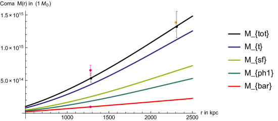
Figure 4: Contribution of the baryonic mass $M_{bar}$, of the scalar field and the phantom energies $M_{sf},\,M_{ph\,1}$ to the transparent mass $M_{t}$ and to the total mass $M_{tot}=M_{t}+M_{bar}$ of the Coma cluster in the WST model. Model errors indicated at $r_{500}$, $r_{200}$ (black). Empirical data for $M_{bar}$ (violet dot) and for the empirically determined total mass $M_{500}$ with error bars (violet) from [29]. Additional empirical data at $r_{200}$ (yellowish) from [19].

It shows an encouraging agreement of the observed values $M_{500}$ at $r_{500}=1278\,kpc$ with the prediction of the Weyl geometric halo model $M_{tot}(r_{500})$ (in the range of the observational errors and of model errors).

$$M_{tot}(r_{500})=5.66^{+0.97\atop-0.68}\,,\qquad M_{500}=6.55^{+0.79\atop-0.79}\quad\times 10^{14}\,M_{\astrosun}$$ (80)

Model error bars have been estimated by varying the input data (79) in their respective error intervals:

At the Abell radius $r_{A}=2.14\,Mpc$ (in the convention of [19]) we get the model values

$$M_{tot}(r_{A})\approx 11.9\,,\quad M_{lens}(r_{A})\approx 7.7\quad\times 10^{14}\,M_{\astrosun}$$ (81)

for the dynamical total mass and the lensing mass (76). Due to the net phantom energy the dynamical mass is about 20 % higher than the lensing mass. This is an effect by which the model can, in principle, be tested empirically and discriminated from others. The baryonic masses in the $\beta$ model are $M_{gas}(r_{A})\approx 11.73\times 10^{13}\,M_{\astrosun}$, $M_{\ast}(r_{A})\approx 1.83\times 10^{13}\,M_{\astrosun}$. Thus not only the total mass $M_{tot}(r_{500})$ given by our model agrees with the empirical value $M_{500}$ inside the error bounds; also $M_{A}$ and $M_{200}$ are reasonably well recovered.

This is the case without assuming any component of particle dark matter besides the (real) energy of the scalar field and the (phantom) energy ascribed to the additional acceleration $a_{\varphi}$ induced by the Weylian scale connection. This might still be a coincidence. In order to learn more about the question whether the findings at the Coma cluster are exemplary or not, we have to consider the data of all 19 galaxy clusters, respectively the 17 of the reliable sub-ensemble.

3.6 Halos and total mass for 17(+2) clusters of galaxies

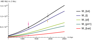
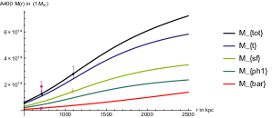
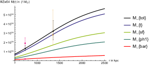
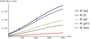
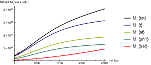
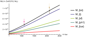
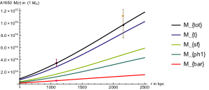
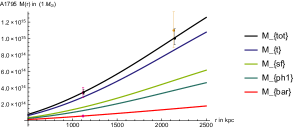
Figure 5: Halo models for clusters 2 – 9 in tab. 1.: total mass $M_{tot}$ (black line) with model error bars at $r_{500},\,r_{200}$, transparent matter halo $M_{t}$ constituted by scalar field halo $M_{sf\,2}$ and net phantom halo (in barycentric rest system of cluster) $M_{ph\,1}$ and baryonic mass (gas and stars) $M_{bar}$. Empirical data for the total mass with error intervals at $r_{500}$ (violet) from [29]. Additional empirical data at $r_{200}$ (yellow) from [19].

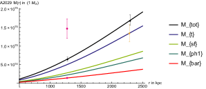
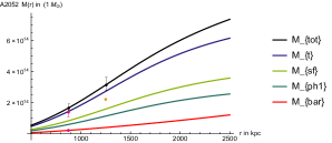
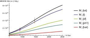
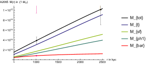
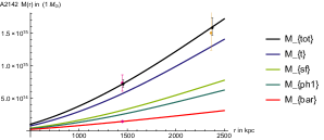
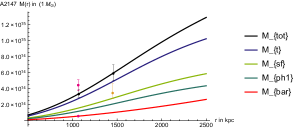
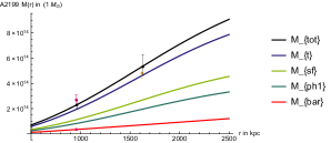
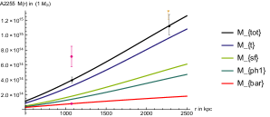
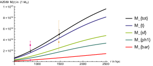
Figure 6: Halo models for clusters 10 – 19 in tab. 1. Description see fig. 5

The mass values of the halo models for the 19 clusters are calculated as described in section 3.3 with the choice of fadeout functions beyond $r=r_{200}$ (see appendix). The results are documented in tables 2, 3 and figs. 5, 6 (for Coma see fig. 4). The baryonic masse at $r_{200}$ ($M_{gas}(r_{200}),M_{\ast}(r_{200})$) of table 3 result from an extrapolation of the empirical values at $r_{500}$ given in [29] to $r_{200}$ using the $\beta$-models of section 3.4, item (1), for gas and star mass.

For 15 clusters our model reproduces the total mass at $r_{500}$ correctly, i.e. inside the error margins of data and model. This is achieved without any further adjustable parameter, only on the basis of the parameters for the $\beta$-model for baryonic mass and $M_{gas}(r_{500}),M_{\ast}(r_{500})$. The fading out functions do not intervene below $r_{200}$. Moreover, for the majority of these, and paradoxically for all other four, the less precisely determined data at $r_{200}$ have overlapping $1\sigma$ error intervals. This indicates a surprising agreement between the (theoretically derived) transparent halo and the empirically determined dark halo, $M_{t}\approx M_{dm}$.

For 5 clusters, A85, A2255, A2589 and the outliers A2029, A2065, the error intervals of empirical data and model data do not overlap. For the first three of them (A85, A2255, A2589) the model predictions are consistent with the empirical data within doubled error intervals ($2\sigma$ range). Only the two outliers (A2029, A2065) lie farther apart. Otherwise the model data are in good agreement with an assumption of normally distributed statistical errors and with the assumption that the evaluation bias due to the use of the NFW profile for dark matter (item (3) in section 3.2) does not shift the mass estimates outside the error intervals.

All in all, the assessment of the WST-3L halo model has surprisingly well passed, in spite of the main caveat of item (3), section 3.2. The outcome found for Coma seems to be typical also for the other clusters. Moreover, the good agreement of the model with the data of the reliable sub-ensemble of 17 clusters supports the assumption stated in the last phrase (3), section 3.2 (no large systematic errors due to data transfer from Einstein/$\Lambda CDM$ to the WST-3L framework). But still we cannot exclude the possibility of cancelling between model errors and data transfer errors. Thus we have only found empirical support for the conjecture that, on the level of galaxy clusters, the observed dark matter effects encoded in $M_{dm}$ may solely be due to the combined impact of the halo $M_{sf}$ of the scalar field and of the scale connection, $M_{ph\,1}$ (cf. (75)):

$$M_{dm}\approx M_{sf}+M_{ph\,1}=M_{t}\qquad$$ (82)

Table 2. Empirical values ($M_{500},M_{200}$) and model values ($M_{tot}$) for total mass at $r_{500},\,r_{200}$
Cluster $r_{500}$ $M_{tot}(r_{500})$ $M_{500}$ $r_{200}$ $M_{tot}(r_{200})$ $M_{200}$ Coma 1278. 5.32 ${}^{+0.83\atop-0.58}$ 6.55 ${}^{+0.79\atop-0.79}$ 2300. 13.19 ${}^{+2.36\atop-1.65}$ 13.84 ${}^{+1.49\atop-1.41}$ A85 1216. 4.67 ${}^{+0.51\atop-0.36}$ 6.37 ${}^{+1.00\atop-1.00}$ 1900. 9.70 ${}^{+1.09\atop-0.77}$ 7.71 ${}^{+0.8\atop-0.74}$ A400 712. 1.26 ${}^{+0.25\atop-0.16}$ 1.83 ${}^{+0.39\atop-0.39}$ 1093. 2.62 ${}^{+0.55\atop-0.35}$ 1.48 ${}^{+0.21\atop-0.18}$ IIIZw54 731. 1.33 ${}^{+0.34\atop-0.27}$ 1.91 ${}^{+0.58\atop-0.58}$ 1350. 3.09 ${}^{+1.30\atop-1.02}$ 2.81 ${}^{+2.74\atop-1.10}$ A1367 893. 1.82 ${}^{+0.29\atop-0.19}$ 1.76 ${}^{+0.27\atop-0.54}$ 1529. 4.28 ${}^{+0.81\atop-0.62}$ 4.06 ${}^{+0.45\atop-0.40}$ MKW4 580. 0.54 ${}^{+0.09\atop-0.06}$ 0.50 ${}^{+0.14\atop-0.14}$ 857. 1.10 ${}^{+0.19\atop-0.13}$ 0.71 ${}^{+0.07\atop-0.06}$ ZwCl215 1098. 3.74 ${}^{+0.47\atop-0.32}$ 4.93 ${}^{+0.98\atop-0.98}$ 2093. 9.32 ${}^{+1.49\atop-1.07}$ 10.37 ${}^{+3.51\atop-2.62}$ A1650 1087. 3.42 ${}^{+0.63\atop-0.50}$ 3.44 ${}^{+0.66\atop-0.66}$ 2150. 9.40 ${}^{+2.87\atop-2.31}$ 11.14 ${}^{+5.77\atop-3.46}$ A1795 1118. 3.40 ${}^{+0.40\atop-0.26}$ 3.41 ${}^{+0.63\atop-0.63}$ 2136. 9.32 ${}^{+1.11\atop-0.74}$ 10.99 ${}^{+2.26\atop-2.09}$ MKW8 715. 0.86 ${}^{+0.18\atop-0.14}$ 0.62 ${}^{+0.12\atop-0.12}$ 1279. 2.35 ${}^{+0.67\atop-0.54}$ 2.38 ${}^{+1.04\atop-0.59}$ A2029 1275. 6.39 ${}^{+0.61\atop-0.43}$ 14.7 ${}^{+2.61\atop-2.61}$ 2286. 15.83 ${}^{+1.57\atop-1.12}$ 13.42 ${}^{+2.43\atop-2.26}$ A2052 875. 1.63 ${}^{+0.26\atop-0.17}$ 1.39 ${}^{+0.28\atop-0.28}$ 1250. 2.94 ${}^{+0.47\atop-0.32}$ 2.21 ${}^{+0.06\atop-0.08}$ MKW3S 905. 1.90 ${}^{+0.27\atop-0.18}$ 1.45 ${}^{+0.34\atop-0.34}$ 1450 3.81 ${}^{+0.60\atop-0.40}$ 3.46 ${}^{+0.36\atop-0.34}$ A2065 1008. 3.92 ${}^{+0.72\atop-0.66}$ 11.18 ${}^{+1.78\atop-1.78}$ 2450. 11.90 ${}^{+8.20\atop-4.61}$ 16.69 ${}^{+21.34\atop-6.73}$ A2142 1449. 7.15 ${}^{+0.68\atop-0.50}$ 7.36 ${}^{+1.25\atop-1.25}$ 2364. 15.29 ${}^{+1.53\atop-1.14}$ 15.03 ${}^{+3.9\atop-2.64}$ A2147 1064. 3.32 ${}^{+0.53\atop-0.40}$ 4.44 ${}^{+0.67\atop-0.67}$ 1450 5.81 ${}^{+1.14\atop-0.90}$ 3.46 ${}^{+1.17\atop-0.74}$ A2199 957. 2.26 ${}^{+0.38\atop-0.28}$ 2.69 ${}^{+0.42\atop-0.42}$ 1621. 4.98 ${}^{+0.93\atop-0.67}$ 4.81 ${}^{+0.37\atop-0.36}$ A2255 1072. 3.94 ${}^{+0.44\atop-0.31}$ 7.13 ${}^{+1.38\atop-1.37}$ 2271. 12.27 ${}^{+1.87\atop-1.37}$ 13.32 ${}^{+1.44\atop-1.19}$ A2589 848. 1.92 ${}^{+0.33\atop-0.22}$ 3.03 ${}^{+0.75\atop-0.75}$ 1471. 4.60 ${}^{+0.84\atop-0.58}$ 3.58 ${}^{+3.86\atop-1.54}$
Model values $M_{tot}(r_{N00})$ and empirical values $M_{N00}$ in $10^{14}\,M_{\astrosun}$,
$r_{N00}$ (empirical) in $kpc$ ($N=1,\,2$)

Table 3. Model values for halo and baryonic masses at $r_{200}$
Cluster $M_{t}$ $M_{sf}$ $M_{sf2}$ $M_{ph1}$ $M_{gas}$ $M_{\ast}$ $f_{\ast}$ $f_{t}$ Coma 11.15 6.44 1.73 4.71 1.77 0.276 0.16 6.3 A85 8.03 4.52 1.01 3.51 1.54 0.140 0.09 5.2 A400 2.27 1.36 0.45 0.91 0.26 0.084 0.32 8.7 IIIZw54 2.77 1.65 0.54 1.11 0.25 0.080 0.32 10.9 A1367 3.77 2.21 0.65 1.56 0.42 0.089 0.21 8.9 MKW4 0.99 0.58 0.18 0.40 0.09 0.022 0.25 10.9 ZwCl215 8.00 4.55 1.11 3.45 1.19 0.137 0.12 6.7 A1650 8.15 4.69 1.24 3.45 1.10 0.162 0.15 7.4 A1795 8.04 4.59 1.14 3.45 1.15 0.14 0.12 7.0 MKW8 2.12 1.24 0.36 0.88 0.20 0.039 0.20 10.8 A2029 12.83 7.15 1.47 5.68 2.83 0.203 0.07 4.5 A2052 2.58 1.50 0.43 1.07 0.31 0.059 0.19 8.3 MKW3S 3.35 1.95 0.55 1.40 0.39 0.072 0.18 8.5 A2065 10.28 5.80 1.32 4.48 1.48 0.142 0.10 6.9 A2142 12.55 6.95 1.35 5.60 2.59 0.159 0.06 4.8 A2147 4.83 2.77 0.71 2.06 0.87 0.118 0.14 5.5 A2199 4.36 2.52 0.68 1.84 0.55 0.088 0.16 8.0 A2255 10.35 5.84 1.33 4.51 1.76 0.166 0.09 5.9 A2589 3.99 2.33 0.68 1.65 0.52 0.105 0.20 7.7
Mass values in $10^{14}\,M_{\astrosun}$, $f_{\ast}=\frac{M_{\ast}}{M_{gas}},\,f_{t}=\frac{M_{t}}{M_{gas}}(r_{200}),$
$r_{200}$ see tab. 2

3.7 Comparison with TeVeS and NFW halos

It is surprising that in the WST-3L approach the total amount of observed dark matter $M_{dm}$ seems to be explained by the energy of the scalar field and the phantom halo, $M_{t}=M_{sf}+M_{ph\,1}$, $M_{dm}\approx M_{t}$. No missing mass is left. In usual relativistic MOND approaches this is not the case for clusters, although it is essentially so for galaxies [10]. Based on a study of about 40 galaxy clusters, R Sanders has proposed the hypothesis of a neutrino component “between a few times $10^{13}$ and $10^{14}\,M_{\astrosun}$”, mostly concentrated close to the center of the cluster, in a region up to twice the core radius, supplementing the baryonic mass and the phantom energy of the TeVeS model [21, p. 902]. In our approach, this hypothesis is unnecessary. Where does this difference arise from?

A model calculation for the Coma cluster, evaluating (57) for the transition function $\mu_{2}=x(1+x^{2})^{-\frac{1}{2}}$ (53) and the corresponding $\nu_{2}$ (54) used by Sanders in [21], shows that the neutrino core had to be tuned to $M_{\nu}\approx\-1.8\times 10^{14}\,M_{\astrosun}$ in order to give agreement with the empirical value $M_{dm}(r_{500})=M_{500}-M_{bar}(r_{500})\approx 4.7\times 10^{14}\,M_{\astrosun}$, where in this framework “$r_{500}$”, “$r_{200}$” are to be defined by a formal convention with regard to a (fictitious) NFW halo.

Table 3 shows the amount of scalar field energy up to a radius $r\approx r_{200}$ in the WST model. It varies between about $2\times 10^{13}$ and $9\times 10^{14}\,M_{\astrosun}$, i.e., roughly in the range found necessary by R. Sanders for the (hypothetical) neutrino halo. Moreover, a comparison of the transition functions $\mu_{w}(r)$ (55) and $\mu_{2}(x)$ shows that the gross phantom energy $\rho_{t}$ of the WST approach is larger than in an $\mu_{2}$-MOND model [24]. Roughly half of the missing mass of Sanders’ model is covered by this effect, the other half is due to the scalar field halo of the system of galaxies up to $r_{200}$.

A comparison of the two MOND-like approaches is given in fig. 7. Here one has to keep in mind that the TeVeS-$\mu_{2}$ model has a free adaptable parameter (mass of the neutrino core), while the WST has not. The general profiles of the “dark matter” halos of both models are similar. The TeVeS-$\mu_{2}$ mass starts from a higher socle because of its neutrino core; the WST transparent mass starts from a lower initial value but rises faster because of the increasing contribution of the scalar field halo of the galaxies.

On the other hand, the best known profile for dark matter distribution, used in most structure formation simulations, is the NFW halo (Navarro/ Frank/White). Its profile is

$$\rho(r)=\frac{\rho_{o}}{\frac{r}{r_{c}}(1+\frac{r}{r_{c}})^{2}}\;,$$ (83)

with density parameter $\rho_{o}$ and core radius $r_{c}$ (at which the density has reduced to half the reference value). For a first comparison of the interior halos we take $r_{c}\approx 180\,h^{-1}\,kpc$ ($h=0.7$), following [14], and determine the central density parameter $\rho_{o}$ such that the total integrated mass $M_{NFW}$ assumes the empirical value of [28] at $r_{500}=1289\,kpc$ (fig. 7). The error intervals for $r_{500}$ give upper and lower model values for $\rho_{o}$ and corresponding model error bars (red) for $M_{NFW}(r_{200})$. This version of the NFW halo satisfies one set of empirical data by construction (at $r_{500}$); our main interest thus goes to the other empirical data set available at $r_{200}=2300\,kpc$. The NFW model error interval overlaps with the empirical error bar at $r_{200}$ and with the error interval of the WST model.

There is a conspicuous difference between the mass profiles of the NFW halo on one side and the halo profiles of WST or $\mu_{2}$-TeVeS on the other. More and precise empirical data of the interior halos of galaxy clusters ought to be able to discriminate between the two model classes. An empirical discrimination between the two MOND-like approaches would need more, and more precise, profile data. At the moment the Weyl MONDlike model survives the comparison fairly well, even though it has no free parameter which would allow to adapt it to the halo data.

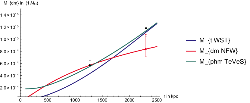
Figure 7: Comparison of dark/transparent/phantom mass halos for Coma in NFW, WST and TeVeS models,   free parameters of halos for NFW and TeVeS ($\mu_{2}$ with neutrino core) adapted to mass data (black error bars) at $r_{500}=1280\,kpc$

3.8 A side-glance at the bullet cluster

At the end of this section let us shed a side-glance at the bullet cluster 1E0657-56. It is often claimed that the latter provides direct evidence in favour of particle dark matter and rules out alternative gravity approaches. Our considerations show that this argument is not compelling. The energy content of the scalar field halos of the colliding clusters endows them with inertia of their own. The shock of the colliding gas exerts dynamical forces on the gas masses only, not directly on the scalar field halos. During the encounter the halos will roughly follow the inertial trajectories of their respective clusters before collision, and they will continue to do so for a while. It will take time before a re-adaptation of the mass systems and the respective scalar field halos has taken place. Clearly the MOND-approximation is unable to cover such violent dynamical processes. It describes only the relatively stable states before collision and – in some distant future – after collision. But a separation of halos and gas masses for a (cosmically “short”) period is to be expected, just like in the case of a particle halo with appropriate clustering properties.

For the time being, the cluster 1E0657-56 does not help to decide between the overarching alternative research strategies, particle dark matter or alternative gravity. It may be able to do so, once the dynamics of gas and of the halos has been modeled with sufficient precision in both approaches. Then a proper comparison can be made. But that is an overtly complicated task. It seems more likely that other types of empirical evidence will offer a simpler path to a differential evaluation of the two strategies and help clarifying the alternative.

4 Discussion

We have analyzed a three-component halo model for clusters of galaxies, consisting of

• the scalar field energy induced by the overall baryonic matter in the barycentric rest system of a cluster (under abstraction of the discrete structure of the star matter clustering in freely falling galaxies) (69), with integrated mass equivalent $M_{sf\,1}$,

• an additional contribution to the scalar field energy, forming around the freely falling galaxies (71), integrating to $M_{sf\,2}$,

• and the phantom energy of the total baryonic mass in the barycentric rest system of the cluster, due to the additional acceleration of the Weylian scale connection in Einstein gauge (70) with mass equivalent $M_{ph\,1}$.

The first two components add up to a real energy content of the scalar field with mass equivalent $M_{sf}=M_{sf\,1}+M_{sf\,2}$, the third one, $M_{ph\,1}$, arises from a theoretical attribution in a Newtonian perspective and has fictitious character. The mass equivalent of the integrated energy components combines to a total dark-matter-like quantity $M_{t}=M_{sf\,1}+M_{sf\,2}+M_{ph\,1}$ (73).

All three components arise from gravitational effects of the cluster’s baryonic mass $M_{bar}=M_{gas}+M_{star}$ in the framework of a Weyl geometric scalar tensor theory of gravity (1), with its scale connection as the specific difference to Riemannian geometry (8), (4). A second speciality of the theoretical framework is the cubic kinetic term of the Lagrangian (28), analogue to the AQUAL approach but in scale covariant form. Observable quantities are directly given by the model in Einstein gauge (9).

The total dynamical mass of the model, $M_{tot}=M_{bar}+M_{t}$ (75) has been heuristically confronted with the empirical values for of 17+2 galaxy clusters given in [26], [28], [29], complemented by data from [19]. The problem of data transfer between different theoretical frameworks (in particular between Einstein gravity /$\Lambda CDM$ and WST-3L) leads to a certain caveat with regard to an uncorrected taking over of the values for the total mass. But it does not seem to obstruct a meaningful first comparison of the WST halo model with available mass data of clusters collected in the Einstein/$\Lambda CDM$ framework.

The result of this comparison shows a surprisingly good agreement of the total mass predicted by the model $M_{tot}$, on the basis of data for the baryonic mass components, with the observed total mass $M_{500}$ (measured at the main reference distance $r_{500}$). Moreover the model shows an acceptably good agreement with additional empirical values at the distance $r_{200}$ given in [19] (determined on a slightly less refined data basis and evaluation method). For 14 clusters the model predicts values for $M_{tot}(r_{500})$ with error intervals (due to the observational errors for the baryonic data) which overlap with the empirical error intervals of $M_{500}$. The Coma cluster is among them. Three clusters have overlapping error intervals in the $2\sigma$ range. The remaining two are outliers and have been identified as such already in [28].

In the result we have found empirical support for conjecturing that the observed dark matter at galaxy cluster level may be due to the transparent halo of the scalar field and the phantom halo of the scale connection of WST (82).

Details for the constitution of the total transparent matter halo from its specific components $(i),\,(ii),\,(iii)$ have been investigated for the Coma cluster (section 3.5). They seem to be exemplary for the whole collection of galaxy clusters. A particular feature of the model is the scalar field energy formed in the inter-spaces between the galaxies. Its integrated energy contribution surpasses the baryonic mass between 1 and 1.5 $Mpc$ (see fig. 3 and table 3, col. 4). It is crucial for this model’s capacity to explain the total dynamic mass on purely gravitational grounds, without any additional dark matter component. An overall comparison with R. Sanders’ TeVeS-MOND model for galaxy clusters and the NFW halo is given in section 3.7.

At the moment the Weyl geometric scalar tensor model with a cubic term in the kinetic Lagrangian of the scalar field fares well in all the mentioned respects. It would be very helpful if astronomers decided to evaluate old or new raw data in the framework of WST. That could lead to an empirical discrimination of the different models. But already independent of the outcome of such a revision, the scalar field $\phi$ and the scale connection $\varphi_{\mu}$ of WST have a remarkable property from a theoretical point of view. They complement the classical Einstein-Riemannian expression for the gravitational structure, the metric field $g_{\mu\nu}$, by a feature which carries a proper energy-momentum tensor (35), (36). The energy momentum of the scalar field plays a crucial role for the constitution of the transparent matter halo. In the present approach it seems to express the self-energy of the extended gravitational structure. It remains to be seen whether this is more than a model artefact.

5 Appendix

5.1 Energy component of the scalar field

In scalar field (Einstein) gauge $D_{\nu}\phi=\partial_{\nu}\phi-\varphi_{\nu}\phi\doteq-\phi\varphi_{\nu}\doteq\phi\partial_{\nu}\omega\doteq\phi D_{\nu}\omega$, and $D_{\nu}\phi^{2}=2\phi D_{\nu}\phi\doteq 2\phi^{2}\partial_{\nu}\omega$. Simliarly

$$D_{\mu}D^{\nu}\phi^{2}\doteq 2D_{\mu}(\phi^{2}\partial^{\nu}\omega)\doteq 2(D_{\mu}\phi^{2}\partial^{\nu}\omega+\phi^{2}D_{\mu}\partial^{\nu}\omega)\,.$$

Moreover,

$$D_{\mu}\partial^{\nu}\omega=\nabla_{\mu}\partial^{\nu}\omega-2\varphi_{\mu}\partial^{\nu}\omega=_{g}\nabla_{\mu}\partial^{\nu}\omega+\delta_{\mu}^{\nu}\varphi_{\lambda}\partial^{\lambda}\omega+\delta_{\lambda}^{\nu}\varphi_{\mu}\partial^{\lambda}\omega-g_{\mu\lambda}\varphi^{\nu}\partial^{\lambda}\omega+2\partial_{\mu}\omega\partial^{\nu}\omega$$

leads to

$$D_{\mu}D^{\nu}\phi^{2} \doteq 2\phi^{2}(2\partial_{\mu}\omega\partial^{\nu}\omega+_{g}\nabla_{\mu}\partial^{\nu}\omega+2\partial_{\mu}\omega\partial^{\nu}\omega-\delta_{\mu}^{\nu}\,\partial_{\lambda}\omega\partial^{\lambda}\omega)$$

$$\doteq 2\phi^{2}(_{g}\nabla_{\mu}\partial^{\nu}\omega+4\partial_{\mu}\omega\partial^{\nu}\omega-\delta_{\mu}^{\nu}\,\partial_{\lambda}\omega\partial^{\lambda}\omega)\,.$$

Thus

$$D_{\lambda}D^{\lambda}\phi^{2}\doteq 2\phi^{2}\,_{g}\nabla_{\lambda}\partial^{\lambda}\omega$$ (84)

Following (35), (36), (33), the energy momentum of the scalar field,

$$\Theta=\theta^{(I)}+\theta^{(II)}=(\xi\phi)^{2}\,T^{(\phi)}=(\xi\phi)^{2}\,(T^{(I)}+T^{(II)})\,,$$

becomes

$$T^{(I)} \doteq -(8\pi G)^{-1}\left(2\,_{g}\nabla_{\lambda}\partial^{\lambda}\omega-3\,\partial_{\lambda}\omega\partial^{\lambda}\omega-\frac{2}{3}\tilde{a}_{o}|\nabla\omega|^{3}+\frac{\lambda}{4}H^{2}\right)\,g$$

$$T_{\mu\nu}^{(II)} \doteq \xi^{2}D_{\mu}D_{\nu}\phi^{2}-2\frac{\partial L_{\phi}}{\partial g^{\mu\nu}}$$

$$\doteq (8\pi G)^{-1}\left({}_{g}\nabla_{\mu}\partial_{\nu}\omega+(1-\tilde{a}_{o}|\nabla\omega|)\partial_{\mu}\omega\partial_{\mu}\omega-\partial_{\lambda}\omega\partial^{\lambda}\omega\,g_{\mu\nu}\right)\,.$$

In the static case the first two terms of $T_{\mu\nu}^{(II)}$ vanish and the total energy component of the scalar field turns into

$$T_{oo}^{\phi}\;\doteq\;(4\pi G)^{-1}\left({}_{g}\nabla_{\lambda}\partial^{\lambda}\omega-\partial_{\lambda}\omega\partial^{\lambda}\omega-\frac{1}{3}\tilde{a}_{o}|\nabla\omega|^{3}+\frac{\lambda}{8}H^{2}\right)\,.$$ (85)

Assuming conditions under which the terms of cosmological orders of magnitude and those of order $|\nabla\omega|^{2}$ can be neglected, we arrive at

$$T_{oo}^{\phi}\;\dot{\approx}\;(4\pi G)^{-1}\,_{g}\nabla_{\lambda}\partial^{\lambda}\omega\,,$$

like in equation (46) of the main text. In the central symmetric case (44) implies $\omega(r)=\sqrt{GM\tilde{a}_{o}}\ln r$. In spherical coordinates $\nabla\omega=(0,\frac{\sqrt{GM\tilde{a}_{o}}}{r},0,0)$ and

$$\nabla^{2}\omega=_{g}\nabla_{\lambda}\partial^{\lambda}\omega\doteq\frac{\sqrt{GM\tilde{a}_{o}}}{r^{2}}$$ (86)

Because of $\partial_{1}\omega\partial_{1}\omega=\frac{GM\tilde{a}_{o}}{r^{2}}\ll\frac{\sqrt{GM\tilde{a}_{o}}}{r^{2}}$ the approximation (46) is justified.

5.2 Remarks on the numerical implementation

The calculations in sections 3.2ff. have been implemented in Mathematica 10 and run on a PC. Integrations of the mass values have been realized by numerical interpolation routines in distance intervals of $100\,kpc$. A comparison with refined distance intervals $10\,kpc$ showed differences at the order of magnitude $10^{-4}$ of the respective values, thus below the rounding precision.

The fading out for the scalar field and phantom halos beyond $r_{200}$ has been modeled by the cubic expression:

$$f(x,A,B)=\chi(x;-\infty,A)+\left(\frac{1}{1+\frac{x-A}{B}}\right)^{3}\chi(x;A,\infty)\,,$$ (87)

with $\chi(x;a,b)$ the characteristic function of the interval $[a,b]$. The fading out of $f(x,A,B)$ starts at $A$ and declines to $\frac{1}{2}$ at $A+B$. In our case we start the fading out close to the virial radius, $A=1.1\,r_{200}$ and set $B=0.5\,r_{200}$.

References

- [1]
- Adler [1975] Adler, Ronald; Bazin, Maurice; Schiffer Menahem. 1975. Introduction to General Relativity. New York etc.: Mc-Graw-Hill. 2nd edition.
- Audretsch [1984] Audretsch, Jürgen; Gähler, Franz; Straumann Norbert. 1984. “Wave fields in Weyl spaces and conditions for the existence of a preferred pseudo-riemannian structure.” Communications in Mathematical Physics 95:41–51.
- Bekenstein [2004] Bekenstein, Jacob. 2004. “Relativistic gravitation theory for the modified Newtonian dynamics paradigm.” Physical Review D 70(083509).
- Bekenstein [1984] Bekenstein, Jacob; Milgrom, Mordechai. 1984. “Does the missing mass problem signal the breakdown of Newtonian gravity?” Astrophysical Journal 286:7–14.
- Biviano [2006] Biviano, A.; Murante, G.; Borgani S. e.a. 2006. “On the efficiency and reliability of cluster mass estimates based on member galaxies.” Astronomy & Astrophysics 456:23–26.
- Blagojević [2002] Blagojević, Milutin. 2002. Gravitation and Gauge Symmetries. Bristol/Philadelphia: Institute of Physics Publishing.
- Brans [1961] Brans, Carl; Dicke, Robert H. 1961. “Mach’s principle and a relativistic theory of gravitation.” Physical Review 124:925–935.
- Drechsler/Tann [1999] Drechsler, Wolfgang; Tann, Hanno. 1999. “Broken Weyl invariance and the origin of mass.” Foundations of Physics 29(7):1023–1064. [arXiv:gr-qc/98020vv v1].
- Famaey [2012] Famaey, Benoît; McGaugh, Stacy. 2012. “Modified Newtonian dynamics (MOND): Observational phenomenology and relativistic extensions.” Living Reviews in Relativity 15(10):1–159.
- Faraoni [1999] Faraoni, Valerio; Gunzig, Edgard. 1999. “Einstein frame or Jordan frame.” International Journal of Theoretical Physics 38:217–225.
- Fujii [2003] Fujii, Yasunori; Maeda, Kei-Chi. 2003. The Scalar-Tensor Theory of Gravitation. Cambridge: University Press.
- Gavazzi [2009] Gavazzi, R.; Adami, C. e.a. 2009. “A weak lensing study of the Coma Cluster.” Astronomy & Astrophysics 498(2):L33–L36. arXiv:0904.0220.
- Geller [1999] Geller, M.J.; Diaferio, Antonaldo; Kurtz M.J. 1999. “The mass profile of the Coma galaxy cluster.” Astrophysical Journal 517:L23–L26.
- Jordan [1952] Jordan, Pascual. 1952. Schwerkraft und Weltall. Braunschweig: Vieweg. 2nd revised edtion 1955.
- Nakayama [2014] Nakayama, Yu. 2014. Scale invariance vs conformal invariance Lecture Notes 5th Taiwan School on Strings and Fields. arXiv:1302.0884.
- Poulis [2011] Poulis, Felipe P.; Salim, J.M. 2011. “Weyl geometry as a characterization of space-time.” International Journal of Modern Physics: Conference Series V 3:87–97. arXiv:1106.3031.
- Quiros [2014] Quiros, Israel. 2014. “Scale invariant theory of gravity and the standard model of particles.” Preprint Guadalajara. arXiv:1401.2643.
- Reiprich [2001] Reiprich, Thomas. 2001. “Cosmological Implications and Physical Properties of an X-Ray Flux-Limited Sample of Galaxy Clusters.” Dissertation University Munich.
- Sanders [1999] Sanders, Robert. 1999. “The virial discrepancy in clusters of galaxies in the context of modified Newtonian dynamics.” Astrophysical Journal 512:L23–L26.
- Sanders [2003] Sanders, Robert. 2003. “Clusters of galaxies with modified Newtonian dynamics.” Monthly Notices Royal Astronomical Society 342:901–908.
- Scholz [2005] Scholz, Erhard. 2005. “On the geometry of cosmological model building.” Preprint Wuppertal, arXiv:gr-qc/0511113.
- Scholz [2014] Scholz, Erhard. 2014. Paving the way for transitions – a case for Weyl geometry. To appear in Towards a Theory of Spacetime Theories, ed. D. Lehmkuhl e.a. Basel: Birkhäuser (Springer). arXiv:1206.1559.
- Scholz [2015] Scholz, Erhard. 2015. “MOND-like acceleration in integrable Weyl geometric gravity.” Foundations of Physics, online first, Nov. 2015, arXiv:1412.0430.
- Weinberg [1972] Weinberg, Stephen. 1972. Gravitation and Cosmology: Principles and Applications of the General Theory of Relativity. New York etc.: Wiley.
- Lagana [2011] Zhang, Yu-Ying; Laganá, Tatiana; Reiprich Thomas; Schneider Peter. 2011. “XMM-Newton/Sloan Digital Sky Survey: Star formation efficiency in galaxy clusters and constraints on the matter density parameter.” Astronomical Journal 743(13):11 pages.
- Zhang [2011] Zhang, Y.-Y.; Andernach, H.; Caretta C.A. 2011. “HIFLUGCS: Galaxy cluster scaling relations between X-ray luminosity, gas mass, cluster radius, and velocity dispersion.” Astronomy & Astrophysics 526(A105):38pp.
- Zhang [2011] Zhang, Y.-Y.; Laganá, T.F.; Pierini D.; Puchwein E.; Schneider P.; Reiprich T.H. 2011. “Star-formation efficiency and metal enrichment of the intracluster medium in local massive clusters of galaxies.” Astronomy & Astrophysics 535(A78):11 pages.
- Zhang [2012] Zhang, Y.-Y., Laganá T.F.; Pierini D.; Puchwein E.; Schneider P.; Reiprich T.H. 2012. “Corrigendum to star-formation efficiency and metal enrichment of the intracluster medium in local massive clusters of galaxies.” Astronomy & Astrophysics 544(C3):1 page.