Self-heterodyne detection of the in-situ phase of an atomic-SQUID

Abstract

We present theoretical and experimental analysis of an interferometric measurement of the in-situ phase drop across and current flow through a rotating barrier in a toroidal Bose-Einstein condensate (BEC). This experiment is the atomic analog of the rf-superconducting quantum interference device (SQUID). The phase drop is extracted from a spiral-shaped density profile created by the spatial interference of the expanding toroidal BEC and a reference BEC after release from all trapping potentials. We characterize the interferometer when it contains a single particle, which is initially in a coherent superposition of a torus and reference state, as well as when it contains a many-body state in the mean-field approximation. The single-particle picture is sufficient to explain the origin of the spirals, to relate the phase-drop across the barrier to the geometry of a spiral, and to bound the expansion times for which the in-situ phase can be accurately determined. Mean-field estimates and numerical simulations show that the inter-atomic interactions shorten the expansion time scales compared to the single-particle case. Finally, we compare the mean-field simulations with our experimental data and confirm that the interferometer indeed accurately measures the in-situ phase drop.

I Introduction

Atomtronics focuses on the creation of atomic analogues to electronic devices. Analogues to several electronic components, such as diodes and transistors, have been proposed Seaman et al. (2007), while several other circuit elements have been experimentally realized, including capacitors Lee et al. (2013); Krinner et al. (2015) and spin-transistors Beeler et al. (2013). The atomic version of the rf-superconducting quantum interference device (SQUID) has been realized Ramanathan et al. (2011); Wright et al. (2013); Eckel et al. (2014a), and initial experiments towards the creation of a dc-SQUID have been performed Ryu et al. (2013); Jendrzejewski et al. (2014). Both SQUID devices are formed using a toroidal Bose-Einstein condensate and contain one or more rotating weak links or barriers. Furthermore, creation of an atomic rf-SQUID in a ring-shaped lattice has been proposed Amico et al. (2014); Aghamalyan et al. (2015). Theoretically persistent current states in (quasi) one-dimensional toroidal geometry have been studied extensively Kashurnikov et al. (1996); Kagan et al. (2000); Büchler et al. (2001); Cominotti et al. (2014). Weak links, whether superconducting or atomic, are characterized by the relationship between the current through and the phase across the barrier Likharev (1979). Accurate measurement of this current- phase relationship in the atomic system is crucial for the characterization of atomtronic devices.

Measurement of the in-situ phase of a condensate through interference is a common tool in modern cold-atom physics. Since the first interference between three-dimensional condensates was demonstrated in 1997 Andrews et al. (1997); Castin and Dalibard (1997), several experiments have used interference to infer details about the in-situ phase profile of condensates Simsarian et al. (2000). Vortices in condensates Inouye et al. (2001) and fluctuations brought on by the two-dimensional Berezinskii-Kosterlitz-Thouless phase transition Hadzibabic et al. (2006) have also been detected interferometrically. Interference between two molecular BECs Kohstall et al. (2011) and BECs on an atom chip have also been observed Shin et al. (2005). Recently, interference measurements have been extended to determine the persistent current state in a toroidal condensate Corman et al. (2014); Eckel et al. (2014b). Reference Eckel et al. (2014b) also measured the current-phase relationship of a BEC in a toroidal trap with a rotating barrier, the atomic analogue of an rf-SQUID.

In the experiment of Ref. Eckel et al. (2014b) a single condensate was created in a simply connected trap and subsequently split into two condensates. One condensate was confined in a toroidally shaped “science” trap and the other condensate was confined in a concentric disc-shaped “reference” trap. We will refer to these together as the “target” trap. A schematic and an in-situ image of atoms in a target trap is shown Fig. 1. The science and reference traps were separated by more than 5 $\mu$m, thus atom tunneling between them is negligible and the condensates dephase rapidly because of imperfections in the splitting procedure. Hence, when the two condensates expand and interfere after turning off all trapping potentials, their relative phase is random, thus representing a self-heterodyne measurement Richter et al. (1986). Rotating weak links are only applied to the condensate in the science trap and the other condensate is a phase reference. The current through and the phase drop across the barrier were inferred from the spiral-shaped modulation in the density profile for short expansion times. The number of spiral arms determines the winding number of the persistent current state, while their chirality determines the direction of atom flow.

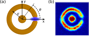
Figure 1: Panel (a) shows a schematic of atoms in a target trap. The inner disc and the outer ring are the reference and science condensates, respectively. A blue-detuned laser forms a rotating weak link and is shown by the blue ellipse. Panel (b) is an in-situ image from the experiment of atoms in a target trap.

In this paper, we study in detail the interference patterns that result from interfering a toroidal condensate with a reference condensate and verify the interferometric technique used in Ref. Eckel et al. (2014b) to measure the current-phase relationship. We first study analytically and numerically a single-particle version of the atomic rf-SQUID in section II. We find that the experimentally observed spirals are a short time phenomenon and both the current through and phase drop across the barrier follow from the geometry of the spirals. For longer expansion times, the spirals become modulated with concentric circles due to self-interference of the torus and it becomes difficult to read out the in-situ phase drop. In Sec. III we describe details of our experiments with sodium condensates in a target trap. In addition, this section describes the numerical techniques used to simulate the mean-field Gross-Pitaevskii equation, which quantifies the effects of atom-atom interactions on the expanding condensates. Estimates of bounds on expansion times, where spirals can be observed in the density profile, are also derived. Finally, a comparison of theoretical and experimental results in Sec. IV validates the interferometric method for measurement of the current-phase relationship of an atom-SQUID.

II Single-particle picture

We begin our study of the interference by deriving analytic expressions for the free expansion of a single atom of mass $m$ released from a target-trap interferometer and give an intuitive explanation of the origin of the spirals in the interference pattern. To generate the interference, we assume that the wavefunction of our single particle is in a superposition of a wave localized in the reference and science regions, respectively.

II.1 Particle in a rotating torus

In order to solve for the wavefunctions, we first describe the target trap in cylindrical coordinates $\vec{x}=(r,\theta,z)$. The science and reference traps are assumed to be parabolic in the radial direction, and centered at $r_{S}$ and the origin, respectively (see Fig. 1(a)). The harmonic oscillator lengths are $\sigma_{S}$ and $\sigma_{R}$, respectively. The common transverse confinement is harmonic with oscillator length $\ell_{z}$. We assume $\sigma_{R}\approx\sigma_{S}$ and $\sigma_{S},\sigma_{R},\ell_{z}\ll r_{S}$. In addition, the science trap has a barrier or weak link rotating at angular frequency $\Omega$ inducing atom flow. For simplicity, we model the barrier in the science trap as a Dirac delta-function $V_{b}(\vec{x},t)=U_{0}w(r)\delta(\theta-\Omega t)$ with strength $U_{0}$, time $t$, and $w(r)$ is a window function which is one around the radial position of the science trap and zero everywhere else.

In the frame rotating with the barrier the atom is prepared in the time-independent state $\Psi_{\rm init}(\vec{x})=(\psi_{R}(\vec{x})+\psi_{S}(\vec{x}))/\sqrt{2}$, where the $\psi_{i}(\vec{x})=\eta_{i}(r)\varphi_{i}(\theta)\phi_{z}(z)$ are separable wave functions of the science ($i=S$) and reference ($i=R$) trap. Here, $\phi_{z}(z)$ is the unit-normalized 1D ground state harmonic-oscillator wavefunction and $\eta_{i}(r)=e^{-(r-r_{i})^{2}/(2\sigma_{i}^{2})}/{\cal N}$ is the radial wavefunction, where ${\cal N}$ is a normalization constant. The overlap between the $\psi_{i}(\vec{x})$ is negligible.

The angular functions $\varphi_{i}(\theta)$ are $1/\sqrt{2\pi}$ for the reference trap and the ground state of the Schrödinger equation $[-d^{2}/d\theta^{2}+2i\kappa d/d\theta+U\delta(\theta)]\varphi_{S}(\theta)=E\varphi_{S}(\theta)$ for the toroidal trap with rotating barrier. Here, $\kappa=\Omega/\Omega_{0}$, $U=U_{0}/{\cal E}_{0}$, $\Omega_{0}=2{\cal E}_{0}/\hbar$, and ${\cal E}_{0}=\langle\hbar^{2}/(2mr^{2})\rangle\approx\hbar^{2}/(2mr_{S}^{2})$ is the natural energy scale of the science trap, where the bracket $\langle\cdot\rangle$ indicates an expectation value over $r$ and $z$ and $\hbar$ is the reduced Planck’s constant. The function $\varphi_{S}(\theta)$ is periodic on $\theta\in[-\pi,\pi]$ and a superposition of $\exp[i(\kappa\pm\sqrt{E+\kappa^{2}})\theta]$ with energy $E=-\kappa^{2}+\epsilon(\kappa)$, where $\epsilon(\kappa)$ is periodic in $\kappa$ with period one. Examples of the phase and magnitude of $\varphi_{S}(\theta)$ are shown in Fig. 2. For most $\kappa$ the phase of $\varphi_{S}(\theta)$ changes nearly linearly with $\theta$. Only for $\kappa\approx 1/2$ and, in fact, near any half-integer $\kappa$ it changes rapidly near the barrier at $\theta=0$. This rapid change around $\theta\in(-\theta_{0},\theta_{0})$ is accompanied by a decrease in density. The phase jump is $\pi(-\pi)$ for $\kappa$ just above (below) $1/2$ and the density is zero at $\theta=0$ for $\kappa=1/2$.

We define the phase drop across the barrier as $\gamma=2\pi(n-s)$, where $n$ is the winding number, which for the ground-state of the single-particle wavefunction equals to the integer closest to $\kappa$, and the slope

$$s=\left.\frac{d}{d\theta}\left[\arg(\varphi(\theta))\right]\right|_{\theta=-\pi}.$$ (1)

A graphical representation of $\gamma$ for $\kappa=0.51$ is shown in Fig. 2. In the rotating frame, the angular current

$$J(\kappa)=r_{S}\Omega_{0}|\varphi_{S}(\theta)|^{2}\left(\frac{d\arg[\varphi_{S}(\theta)]}{d\theta}-\kappa\right),$$ (2)

for any $\theta$ and we used the fact that $\langle 1/r\rangle=1/r_{S}$.

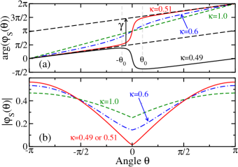
Figure 2: Phase (panel a) and magnitude (panel b) of the single-particle ground-state angular wavefunction $\varphi_{S}(\theta)$ as a function of $\theta$ for various values of rotation rate $\kappa$. The wavefunction is calculated in the frame rotating with a delta-function potential of strength $U_{0}=1$ located at $\theta=0$. For $\kappa\approx 1/2$, a sharp change in the phase occurs in the $\kappa$-dependent region $\theta\in(-\theta_{0},\theta_{0})$. The figure also shows the phase-drop $\gamma$, defined in the text, for $\kappa=0.51$.

II.2 Single-particle interference

After turning off the target trap the atomic wavefunction , $\Psi(\vec{x},t)$, freely expands and interferes. At time $t$ after the release, it is imaged along the $z$ axis leading to the observable $n(r,\theta,t)=\int_{-\infty}^{\infty}dz\,|\Psi(\vec{x},t)|^{2},$ where $\Psi(\vec{x},t=0)=\Psi_{\rm init}(\vec{x})$. During the expansion, the wavefunction of the torus and disc remains separable in the $z$ direction, i.e. $\psi_{i}(\vec{x},t)=\chi_{i}(r,\theta,t)\phi_{z}(z,t)$. Thus, $n(r,\theta,t)=|\chi_{R}(r,\theta,t)+\chi_{S}(r,\theta,t)|^{2}$ as $\int dz|\phi_{z}(z,t)|^{2}=1$.

It is convenient to first follow the expansion with a numerical solution of the Schrödinger equation in the $(r,\theta)$ plane for $\kappa$ near $1/2$. Figure 3 shows $n(r,\theta,t)$ for two different expansion times. (Time propagation was carried out by switching to momentum space, applying appropriate time-dependent phase factors, and returning back to coordinate space.) We observe that as soon as the wavefunctions of the two traps overlap, the interference pattern consists of spirals. Later on, the self-interference of the science wavefunction yields circles superimposed on the spirals.

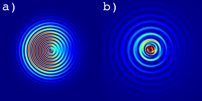
Figure 3: Numerical simulation of the integrated particle density $n(r,\theta,t)$ of a single particle, with winding number equal to one, expanding in the rotating frame after release from a target trap. Panel (a) shows $n(r,\theta,t)$ with spirals at an early expansion time $t=0.25\tau_{C}$, evaluated at $r=r_{S}$. Panel (b) shows a later time $t=1.25\tau_{C}$, where the spirals are superimposed with circles due to self-interference of the toroidal wavefunction. The density near the center has been truncated for better contrast. The trap parameters are $\sigma_{R}=0.025r_{S},\,\sigma_{S}=0.05r_{S},\,U_{0}=1$ and $\kappa=0.51$. The length of the sides in panels (a) and (b) corresponds to $5.12r_{S}$ and $12.8r_{S}$, respectively. The parameters are chosen such that the overlap between the expanding science and reference wavefunctions is sufficient to show the spiral over a large range of radii.

We confirm these interference patterns with an asymptotic expansion and study the associated time-scales. The time evolution of the reference state is

$$\chi_{R}(r,\theta,t)=e^{-r^{2}/2\sigma^{2}_{R}(t)}/{\cal N}_{1}(t),$$ (3)

where $\sigma_{R}^{2}(t)=\sigma_{R}^{2}+i\hbar t/m$ and ${\cal N}_{1}(t)$ normalizes the wavefunction. Hence, for $t\gg m\sigma_{R}^{2}/\hbar$ the spatial extent of the reference wavefunction, $\sqrt{|\sigma_{R}^{2}(t)|}$, is proportional to the expansion time, corresponding to ballistic expansion. In contrast, the expanding science wavefunction is not analytically solvable. We can, however, derive an asymptotic series based on the pertinent timescales of the expansion of the science wavefunction. The shortest time scale is the ballistic time $\tau_{B}=m\sigma_{S}^{2}/\hbar$ determined by the initial radial width. In addition, as will become clear later, there are two position-dependent timescales: an intermediate timescale $\tau_{C}(r)=m\sigma_{S}(r+r_{S})/\hbar$ and a long timescale $\tau_{S}(r)=mrr_{S}/\hbar$. We are interested in the expansion time interval $\tau_{B}\ll t\ll\tau_{S}(r)$. Figure 3 shows the density profile for two such times.

Formally, expanding wavefunction $\chi_{S}(r,\theta,t)$ evolves as

$$\chi_{S}(r,\theta,t) =\int_{0}^{\infty}dr^{\prime}\,r^{\prime}\eta_{S}(r^{\prime})$$

$$\times\int_{-\pi}^{\pi}d\theta^{\prime}\,G(r,\theta,r^{\prime},\theta^{\prime},t)\varphi_{S}(\theta^{\prime}),$$ (4)

where the free-particle Green’s function Feynman et al. (2010) in two-dimensions is

$$G(r,\theta,r^{\prime},\theta^{\prime},t) =\frac{m}{2\pi i\hbar t}\times$$ (5)

$$\exp\left\{\frac{im\left[r^{2}+r^{\prime 2}-2rr^{\prime}\cos(\theta-\theta^{\prime})\right]}{2\hbar t}\right\}.$$

We note that the integral over $r^{\prime}$ is concentrated around $r^{\prime}=r_{S}$. Consequently, the integral over $\theta^{\prime}$ in Eq. II.2 can be solved by noting that the phase on the right hand side (RHS) of Eq. 5 oscillates rapidly for $t\ll mrr^{\prime}/\hbar\approx\tau_{S}(r)$. Then, the method of steepest-descent Bender and Orszag (1978) gives an asymptotic series for integral over $\theta^{\prime}$ in powers of the small parameter $t/\tau_{S}(r)$. In fact, there are two stationary points located at $\theta^{\prime}=\theta$ and $\theta^{\prime}=\theta+\pi$, respectively. The remaining integral over $r^{\prime}$ is also solved using steepest descent for $\tau_{B}\ll t$ based on the small parameter $\sigma_{S}/r_{S}$. To leading order we find

$$\chi_{S}(r,\theta,t)= \left[e^{-(r-r_{S})^{2}/[2\sigma^{2}_{S}(t)]}\varphi_{S}(\theta)\right.$$ (6)

$$\left.+\,e^{-(r+r_{S})^{2}/[2\sigma^{2}_{S}(t)]}\varphi_{S}(\theta+\pi)\right]/({\cal N}_{2}(t)\sqrt{r})\,,$$

where the complex, time-dependent $\sigma_{S}^{2}(t)=\sigma_{S}^{2}(1+it/\tau_{B})$ is the square of the width of the expanding radial wave-packet and $1/{\cal N}_{2}(t)$ is a normalization factor. The wavefunction is a superposition of two expanding 1D Gaussians centered at $r_{S}$ and $-r_{S}$ (except for the probability conserving factor $1/\sqrt{r}$). The asymptotic solution is valid for $\tau_{B}\ll t\ll\tau_{S}(r)$. This excludes the region near the origin, where $\tau_{S}(r)$ is small.

It is natural to ask whether the second term in Eq. 6 is important relative to the first term. Clearly, when $\sqrt{|\sigma^{2}_{S}(t)|}<r+r_{S}$ or equivalently $t<\tau_{B}(r+r_{S})/\sigma_{S}=\tau_{C}(r)$ the second term is negligible. The interference of the first term with the reference wavefunction $\chi_{R}(r,\theta,t)$ in Eq. 6 leads to spirals in the density $n(r,\theta,t)$ as shown in Fig. 3(a). For $t\geq\tau_{C}(r)$ the second term cannot be ignored and interferes with the first term. It leads to circles in addition to the spirals as shown in Fig. 3(b). An intuitive interpretation of $\tau_{C}(r)$ is that it corresponds to the time taken by signals from both antipodal points $(r_{S},\theta)$ and $(r_{S},\theta+\pi)$ of the initial $t=0$ wavefunction of the torus to reach the observation point $(r,\theta)$ and interfere. This is the self-interference of the toroidal wavefunction.

II.3 Spirals

We are now in a position to quantify the spiral structure for $\tau_{B}\ll t\ll\tau_{C}$. We write $\chi_{i}(r,\theta,t)=\sqrt{n_{i}(r,\theta,t)}\exp[i\xi_{i}(r,\theta,t)]$, where $n_{i}(r,\theta,t)$ is the probability density and $\xi_{i}(r,\theta,t)$ is the phase. The integrated density becomes

$$n(r,\theta)=n_{S}(r,\theta)+n_{R}(r,\theta)+2\sqrt{n_{S}(r,\theta)n_{R}(r,\theta)}\cos\xi(r,\theta),$$

where $\xi(r,\theta)=\xi_{S}(r,\theta)-\xi_{R}(r)$ and we suppress the time argument for notational simplicity. The last term on the RHS of this equation describes the interference of the wavefunctions in the two traps.

For the above time interval the second term in Eq. 6 can be ignored, so that $n_{R}(r,\theta,t)$ is independent of $\theta$, $n_{S}(r,\theta,t)$ is a separable function of $r$ and $\theta$, and $\xi(r,\theta)\approx\arg[\varphi_{S}(\theta)]-\hbar rr_{S}/(mt)$. (The argument $\arg[\phi_{S}(\theta)]$ is defined as a monotonic function of $\theta$.) Then, spirals correspond to curves of constant phase $\xi(r,\theta)$ in the $(r,\theta)$ plane. The densities $n_{i}(r,\theta)$ only lead to a slowly-varying envelope in $r$ and suppression of the signal near $\theta=0$ that is most pronounced for half-integer $\kappa$. Consequently, a spiral is described by the parametric curve $r(u)=(\xi_{0}+\arg[\varphi_{S}(\theta(u))])\times\hbar t/(mr_{S})$ and $\theta(u)=-\pi+u\mod 2\pi$, where $\xi_{0}$ is a constant (typically chosen such that $n(r,\theta)$ is a local extremum) and $u$ is the free parameter. In the absence of a rotating barrier but for a non-zero winding number $n$ of the toroidal state, we find $\arg[\varphi_{S}(\theta)]=n\theta$ and the interference pattern has Archimedean spirals with $r(u)=(\xi_{0}+nu)\times\hbar t/(mr_{S})$ and $\theta(u)=-\pi+u\mod 2\pi$. These smooth spirals have been observed experimentally Eckel et al. (2014b); Corman et al. (2014).

A schematic of a spiral is shown in Fig. 4 at a single expansion time $t$ for $\kappa$ slightly greater than $1/2$, a case where $\varphi_{S}(\theta)$ has a sharp phase jump across the barrier near $\theta=0$. For $|\theta|>\theta_{0}$ the spirals smoothly wind around the origin. In contrast, for $\theta\in(-\theta_{0},\theta_{0})$ there is a sharp, nearly discontinuous change in the spirals. For $\kappa$ away from half-integer values the spirals are smooth everywhere. The geometry of a spiral is completely determined by the phase $\xi(r,\theta)$ where the number of spiral arms is the winding number $n$. The densities $n_{R}(r,\theta)$ and $n_{S}(r,\theta)$ determine how many windings of a spiral are visible along the radial direction.

We characterize the discontinuity or jump of the spirals by lengths $\delta$ and $\Delta$ shown in Fig. 4. The quantity $\delta=2\pi\hbar t/(mr_{S})$ is the radial fringe spacing and measures the increment in $r$ as $\xi(r,\theta)$ is increased by $2\pi$ at a fixed $\theta$. Moreover, $\Delta=r_{A}(u+2\pi)-r_{A}(u)=s\times 2\pi\hbar t/(mr_{S})$, where we used the Archimedean spiral $r_{A}(u)=(\xi_{0}+su)\times\hbar t/(mr_{S})$ and $\theta_{A}(u)=-\pi+u\mod 2\pi$, and $s$ is defined by Eq. 1. Intuitively, $\Delta$ is the radial distance covered by a spiral when it is smoothly continued across the barrier region. The two lengths depend on the dimensions of the torus and expansion time $t$.

The ratio $\Delta/\delta=s$ is independent of the radial wavefunction and expansion time. In fact, we can interpret $\Delta/\delta$ as a measurement of the phase across the barrier $\gamma$, since

$$\gamma=2\pi(n-\Delta/\delta).$$ (7)

Moreover, it is a measurement of angular current $J(\kappa)$, as the hydrodynamic equation Eq. 2 at $\theta=-\pi$ gives

$$J(\kappa)=r_{S}\Omega_{0}|\varphi_{S}(-\pi)|^{2}\left(\Delta/\delta-\kappa\right).$$ (8)

Figure 4: Schematic of a spiral-like contour (solid line) in the integrated density for $\kappa$ slightly larger than $1/2$, so that the winding number $n=1$. The contour has a constant phase $\xi(r,\theta)=\xi_{0}$. The phase of $\varphi_{S}(\theta)$ varies rapidly in the wedge $\theta\in(-\theta_{0},\theta_{0})$. In addition, a Archimedean spiral (dashed line) with the same initial angular velocity as the solid line is shown. Its parameters as well as the lengths $\delta$ and $\Delta$ are defined in the text.

For $t>\tau_{C}$ radial rings will get superimposed on the spirals due to the self-interference, making extraction of curves of constant $\xi(r,\theta)$ more difficult. Moreover, when $t\sim\tau_{S}(r)$, the derivatives of the initial angular wavefunction become important; finally, for $t\gg\tau_{S}(r)$, the probability distribution resembles the Fourier transform of the initial wavefunction, which has no spirals and the in-situ phase can not be read out.

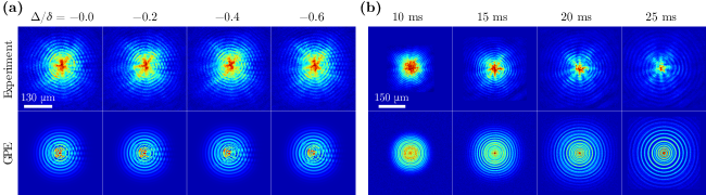
Figure 5: (Color online) Panel a) False color images of the interference pattern in the density profile after a $17$ ms expansion time for four rotation rates of the barrier. The atom number density increases from blue to red with blue corresponding to zero density. Top and bottom rows show images from our experiment and GPE simulations with the same trapping potentials and atom number, respectively. The extracted $\Delta/\delta$ for each rotation rate is shown above the images. The winding number is zero for all images. Panel b) Images of experimental (top) and GPE (bottom) density profiles for four expansion times of a non-rotating condensate released from a target trap without a barrier.

III Experimental atom SQUID and mean-field simulation

We have also performed interference experiments with quantum-degenerate Sodium atoms in a target trap as well as simulations based on the mean-field Gross-Pitaevskii equation (GPE). These results can be compared to our single-particle analysis and show the role of atom-atom interactions present in ultra-cold atomtronic experiments.

The experimental setup is described in Sec. III.1. Details of our numerical methods to simulate the GPE are given in Sec. III.2, while Sec. III.3 describes expansion timescales based on a self-similar expansion of a BEC from a target trap Castin and Dum (1996). Section IV compares our results and enables us to verify the extraction technique used in Ref. Eckel et al. (2014b) for the phase-drop across the barrier in terms of a measurement of $\Delta/\delta$.

III.1 Experimental setup

We have performed interference experiments in a target trap. We create a ${}^{23}\rm{Na}$ BEC in a target trap with approximately $7\times 10^{5}$ atoms and a chemical potential, $\mu/\hbar\approx 2\pi\times(2\mbox{ kHz})$. Details of the creation of the trapping potential can be found in Refs. Eckel et al. (2014a, b). The target trap has an external toroid with a radius of 22.4(4) $\mu$m and radial trapping frequency of 240 Hz. Its central disc has a flat-bottomed potential and contains about 25% of the total atoms. The transverse trapping frequency of both traps is $\approx$ 600 Hz. This leads to a Bose condensate with a measured Thomas-Fermi radial width of about 6 $\mu$m in the toroid and a Thomas-Fermi radius of about 5 $\mu$m in the disc. The barrier potential has a Gaussian profile with a height less than the chemical potential of the atoms in the science trap. Its $1/e^{2}$ full width is $\approx$ 6 $\mu$m. Persistent current states are created by adiabatically ramping up of the height of the barrier with a fixed rotation rate. The atom cloud is imaged along the transverse direction by absorption imaging, which measures the intensity of resonant light transmitted through the expanding gas.

III.2 Numerical simulation

The initial wavefunction, $\Psi_{\rm GP}(\vec{x})$, of the condensate in the target trap is found in a two-step process. We first solve the Gross-Pitaevskii equation for the wavefunction of a BEC with a stationary weak link or barrier but otherwise the same trapping potentials and atom number as in the experiment. We use imaginary-time propagation and a two-dimensional effective Lagrangian Variational Method (2D LVM) Edwards et al. (2012); Pérez-García et al. (1997), assuming a scattering length $a=2.8$ nm. The method is a variational technique whose trial wave function is the product of an arbitrary function in the $(r,\theta)$ plane and a Gaussian in the $z$ direction with an (imaginary-)time-dependent width and a phase that is quadratic in $z$. This Ansatz leads to (a) a two-dimensional effective GPE whose nonlinear coefficient contains the width of the Gaussian and (b) an evolution equation for the width that depends on the spatial integral of the fourth power of the absolute value of the solution of the effective GPE. We denote this solution by $\Psi_{\rm Stat}(\vec{x})$ and normalize such that $\int d^{3}\vec{x}|\Psi_{\rm Stat}(\vec{x})|^{2}=N$, the total atom number. In particular, we can find the angular density profile of the science trap $\rho_{\rm Stat}(\theta)=\int^{\prime}rdrdz|\Psi_{\rm Stat}(r,\theta,z)|^{2}$, where the radial integral only encompasses the science or toroidal trap.

The second step is to add the rotation of the barrier by multiplying the stationary (and positive) $\Psi_{\rm Stat}(\vec{x})$ with a spatially dependent phase that leaves the density profile unchanged, i.e. $\Psi_{\rm GP}(\vec{x})=\Psi_{\rm Stat}(\vec{x})e^{i\zeta(\vec{x})}$. The phase profile $\zeta(\vec{x})$ is zero around and inside the central disk and near the torus only depends on $\theta$. For a given rotation rate $\kappa$ and winding number $n$ it is found by simultaneously solving the hydrodynamic expression $J=r_{S}\Omega_{0}\rho_{\rm Stat}(\theta)(d\zeta(\theta)/d\theta-\kappa)$ and $\zeta(\pi)-\zeta(-\pi)=2n\pi$. (Compare to Eq. 2 as well as see the supplemental material in Ref. Eckel et al. (2014b)). The solution is similar in behavior to those shown in Fig. 2 and the phase drop follows from $\gamma=2\pi(n-s)$, where $s=d\zeta(\theta)/d\theta\mid_{\theta=-\pi}$.

This phase-imprinting procedure is valid as long as the height of the barrier is less than the chemical potential, the healing length $\ell=\sqrt{\hbar/(2m\mu)}\approx 0.5\,\mu\rm m$ is small compared to the width of the barrier ($\approx 6$ $\mu$m), and the speed of the barrier is small compared to the speed of sound $c=\sqrt{\mu/m}$. These conditions are also met in the experiment.

Finally, we simulate the expansion of our BEC wavefunction released from a target-trap by solving the (real) time-dependent Gross-Pitaevskii equation using the same 2D-LVM method. The GPE solutions have only been modified to include the effects of absorption imaging. The non-zero point-spread-function of the imaging system is taken into account by convolving the simulated transmission with an Airy disk of the appropriate size.

III.3 Expansion time scales

References Castin and Dum (1996); Kagan et al. (1996) showed that a harmonically trapped and interacting Bose condensate expands at a much faster rate than an non-interacting gas of the same size. Here, we perform a similar analysis for expansion from a target trap. In fact, under the assumptions valid for phase imprinting in Sec. III.2, it is sufficient to study expansion from a BEC in a toroidal trap without a barrier or rotation. We assume that the interactions are sufficiently strong that the Thomas-Fermi approximation holds along the $r$ and $z$ directions. The BEC wavefunction is then independent of $\theta$ and the harmonic confinement in the toroidal trap along the $r$ and $z$ directions leads to a BEC with Thomas-Fermi radius, $\sigma_{\rm TF}$, such that $\sigma_{\rm TF}\ll r_{S}$. Here, for simplicity we assume the same trap frequency along the two directions, i.e. $\omega_{r}=\omega_{z}\equiv\omega$.

Immediately, after the release of the toroidal trap the BEC expands rapidly in the $r$ and $z$ directions as the interaction energy gets converted to kinetic energy. This defines a ballistic timescale $\tilde{\tau}_{B}$ (We use tilde to denote timescales associated with expansion of the interacting BEC.) As $\sigma_{\rm TF}\ll r_{S}$, we can locally approximate an angular section of the torus as a two dimensional tube, which expands along its transverse directions. Such an elongated BEC undergoes a self-similar expansion Castin and Dum (1996); Kagan et al. (1996). That is, in the hydrodynamic picture of the BEC and cylindrical coordinates, the density is $n(r,z,t)\approx n(r_{S}+(r-r_{S})/\lambda(t),z/\lambda(t),t=0)$ while the velocity field $\vec{v}(\vec{x},t)=(v_{r}(r,t),0,v_{z}(z,t))$ with $v_{r}(r,t)=(1-\lambda(t)^{-2})(r-r_{S})/t$ and $v_{z}(z,t)=(1-\lambda(t)^{-2})z/t$. The scaling factor $\lambda(t)=\sqrt{1+\omega^{2}t^{2}}$, which implies $\tilde{\tau}_{B}=1/\omega=m\sigma_{S}^{2}/\hbar$ and is the same as the single-particle ballistic time $\tau_{B}$, even though the radial size of the BEC wavefunction $\sigma_{\rm TF}\gg\sigma_{S}$.

For $t\gg\tilde{\tau}_{B}$, the interaction energy has been converted to kinetic energy, the density profile has spirals, but the cloud is expanding more rapidly than the single-particle case. Hence, we expect that the time scale, $\tilde{\tau}_{C}(r)$, where the spirals become modulated with circles due to the self-interference of the toroidal BEC, will be shorter than the equivalent single-particle time scale, $\tau_{C}(r)$. We can derive $\tilde{\tau}_{C}$ following the intuitive understanding of signals from antipodal points $(r_{S},\theta)$ and $(r_{S},\theta+\pi)$ at $t=0$ reaching $(r,\theta)$ at $t=\tilde{\tau}_{C}$. In other words, we require that the radial size of the toroidal BEC, $\lambda(\tilde{\tau}_{C})\sigma_{\rm TF}$, is larger or equal to the distance between the observation point and the antipodal points, i.e. $r+r_{S}$ and $r-r_{S}$. Hence, $\tilde{\tau}_{C}\approx(r+r_{S})/(\omega\sigma_{\rm TF})=(\sigma_{S}/\sigma_{\rm TF})\tau_{C}$, which is smaller than $\tau_{C}$.

IV Comparison of the experiment with theory

We compare our experimental data and GPE simulations in Fig. 5 by showing the dependence of the interference pattern on the rotation rate of the barrier and the expansion time. Figure 5a) shows typical expanded clouds at $17$ ms expansion time from our experiment and simulated GPE expansions for various rotation rates of the barrier leading to condensates with winding number $n=0$. Firstly, we see radial interference fringes at fixed $\theta$ and azimuthal interference fringes at fixed $r$ similar to those in Fig. 4. The ratio $\Delta/\delta$ from these experimental images is extracted following the procedure explained in Fig. 4. The phase-drop across and the current through the barrier then follows from Eqs. 7 and 8, respectively. Near $\theta=0$, where the barrier is located before release, the density profile has radial stripes, which are absent from the single-particle simulations and a consequence of interaction-induced expansion of atoms into the density depleted weak-link region. Lastly, star-like structures, which are due to residual azimuthal asymmetries in the toroidal potential, are visible.

Figure 5b) shows expanding, rotationless clouds released from a trap without barrier for various expansion times. For observation radii $r\geq 60$ $\mu$m and small expansion times $t\lesssim 20$ ms, the experimental data and GPE results show no evidence of self-interference of the toroidal BEC consistent with $t\leq\tilde{\tau}_{C}(r)$. For longer expansion times we observe self-interference. It is prominent near the cloud center, where radial fringes emerge with half the spacing of those at large radius.

In Fig. 5 the size, shape and interference pattern of the clouds in the GPE simulations agree well with those of the experiment. The agreement is made quantitative in Fig. 6 for the target trap without a barrier and a BEC without winding ($n=0$). The figure shows the radial fringe spacing, $\delta$, from the experimental data, GPE simulations and the single-particle expression $\delta=2\pi\hbar t/(mr_{S})$ as functions of expansion time. The three cases are in excellent agreement, indicating that this fringe spacing is determined by the geometry of the system, i.e. the radius of the torus.

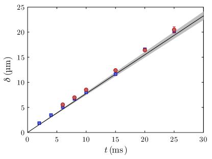
Figure 6: Radial fringe spacing, $\delta$, of the interference pattern as a function of time elapsed after the release of the target trap. The data is for a toroidal trap without a barrier and a BEC without winding. The experimental, GPE and single-particle fringe spacings are shown by red dots with one-standard deviation statistical error bars, blue markers and a black line, respectively. The value of $r_{S}$ has a uncertainty, which is shown by the shaded region around the black line.

Figure 7 shows the extracted $\Delta/\delta$ as a function of the imprinted phase drop $\gamma$ across the barrier for the GPE simulations in Fig. 5a). The result agrees within our uncertainties with the single-particle prediction, which indicates that interactions do not change the phase drop over the barrier region even though the angular density profile is distorted during the expansion. In other words, an extraction of the phase drop from a measurement of $\Delta/\delta$ is valid even when the GPE and experiment have radial stripes for small $\theta$ near the weak link. The latter are absent from the single-particle interference pattern.

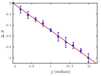
Figure 7: The ratio $\Delta/\delta$ as a function of in-situ phase-drop $\gamma$ across the rotating barrier from the GPE simulations of Fig. 5a) (markers) and the single-particle prediction (solid line). Error bars are one standard deviations uncertainties from the fit to the density profile.

V Conclusion

We have experimentally and theoretically investigated an interferometric measurement of the phase drop in an atomic-SQUID. The atomic-SQUID consists of a BEC in a toroidal trap with a rotating barrier. The phase drop across the barrier is measured by interference with a reference disc BEC after release from the trapping potentials. We have studied the single-particle case and find that the structure of the interference pattern depends on the expansion time after release. For short times, it consists of spirals, which have the same number of arms as the winding number of the toroidal wavefunction. The phase along a spiral is the same as the in-situ phase of the angular wavefunction. Moreover, we find that the phase drop across the barrier and the current through it determine the geometry of spirals. For longer times the spirals get superimposed by circles making phase readout difficult.

The conclusions from the single-particle model are confirmed by experiments with Bose condensed sodium atoms and numerical simulations based on the Gross-Pitaevskii equation even though inter-atomic interactions speed up the expansion, thereby shortening the associated time scales. In particular, one feature that is not changed is the fringe spacings of the interference pattern.

Most importantly, we have confirmed that the phase-drop across the barrier as measured by our experiment agree with those of our single-particle model and mean-field simulations and accurately reflect the in-situ value. This confirmation opens up the possibility of using this technique for measuring the current-phase relationship of, for example, excitations or weak links in degenerate, superfluid Fermi gases.

References

- Seaman et al. (2007) B. T. Seaman, M. Krämer, D. Z. Anderson, and M. J. Holland, Phys. Rev. A 75, 023615 (2007).
- Lee et al. (2013) J. G. Lee, B. J. McIlvain, C. J. Lobb, and I. Hill, W. T., Sci. Rep. 3, 1034 (2013).
- Krinner et al. (2015) S. Krinner, D. Stadler, D. Husmann, J.-P. Brantut, and T. Esslinger, Nature 517, 64 (2015).
- Beeler et al. (2013) M. C. Beeler, R. A. Williams, K. Jiménez-García, L. J. LeBlanc, A. R. Perry, and I. B. Spielman, Nature 498, 201 (2013).
- Ramanathan et al. (2011) A. Ramanathan, K. C. Wright, S. R. Muniz, M. Zelan, W. T. Hill, C. J. Lobb, K. Helmerson, W. D. Phillips, and G. K. Campbell, Phys. Rev. Lett. 106, 130401 (2011).
- Wright et al. (2013) K. C. Wright, R. B. Blakestad, C. J. Lobb, W. D. Phillips, and G. K. Campbell, Phys. Rev. Lett. 110, 025302 (2013).
- Eckel et al. (2014a) S. Eckel, J. G. Lee, F. Jendrzejewski, N. Murray, C. W. Clark, C. J. Lobb, W. D. Phillips, M. Edwards, and G. K. Campbell, Nature 506, 200 (2014a).
- Ryu et al. (2013) C. Ryu, P. W. Blackburn, A. A. Blinova, and M. G. Boshier, Phys. Rev. Lett. 111, 205301 (2013).
- Jendrzejewski et al. (2014) F. Jendrzejewski, S. Eckel, N. Murray, C. Lanier, M. Edwards, C. J. Lobb, and G. K. Campbell, Phys. Rev. Lett. 113, 045305 (2014).
- Amico et al. (2014) L. Amico, D. Aghamalyan, F. Auksztol, H. Crepaz, R. Dumke, and L. C. Kwek, Sci. Rep. 4, 4298 (2014).
- Aghamalyan et al. (2015) D. Aghamalyan, M. Cominotti, M. Rizzi, D. Rossini, F. Hekking, A. Minguzzi, L.-C. Kwek, and L. Amico, New J. Phys. 17, 045023 (2015).
- Kashurnikov et al. (1996) V. A. Kashurnikov, A. I. Podlivaev, N. V. Prokof’ev, and B. V. Svistunov, Phys. Rev. B 53, 13091 (1996).
- Kagan et al. (2000) Y. Kagan, N. V. Prokof’ev, and B. V. Svistunov, Phys. Rev. A 61, 045601 (2000).
- Büchler et al. (2001) H. P. Büchler, V. B. Geshkenbein, and G. Blatter, Phys. Rev. Lett. 87, 100403 (2001).
- Cominotti et al. (2014) M. Cominotti, D. Rossini, M. Rizzi, F. Hekking, and A. Minguzzi, Phys. Rev. Lett. 113, 025301 (2014).
- Likharev (1979) K. Likharev, Rev. Mod. Phys. 51, 101 (1979).
- Andrews et al. (1997) M. R. Andrews, C. G. Townsend, H.-J. Miesner, D. S. Durfree, D. M. Kurn, and W. Ketterle, Science 275, 637 (1997).
- Castin and Dalibard (1997) Y. Castin and J. Dalibard, Phys. Rev. A 55, 4330 (1997).
- Simsarian et al. (2000) J. E. Simsarian, J. Denschlag, M. Edwards, C. W. Clark, L. Deng, E. W. Hagley, K. Helmerson, S. L. Rolston, and W. D. Phillips, Phys. Rev. Lett. 85, 2040 (2000).
- Inouye et al. (2001) S. Inouye, S. Gupta, T. Rosenband, A. P. Chikkatur, A. Görlitz, T. L. Gustavson, A. E. Leanhardt, D. E. Pritchard, and W. Ketterle, Phys. Rev. Lett. 87, 080402 (2001).
- Hadzibabic et al. (2006) Z. Hadzibabic, P. Krüger, M. Cheneau, B. Battelier, and J. Dalibard, Nature 441, 1118 (2006).
- Kohstall et al. (2011) C. Kohstall, S. Riedl, E. R. Sánchez Guajardo, L. A. Sidorenkov, J. Hecker Denschlag, and R. Grimm, New J. Phys. 13, 065027 (2011).
- Shin et al. (2005) Y. Shin, C. Sanner, G.-B. Jo, T. A. Pasquini, M. Saba, W. Ketterle, D. E. Pritchard, M. Vengalattore, and M. Prentiss, Phys. Rev. A 72, 021604 (2005).
- Corman et al. (2014) L. Corman, L. Chomaz, T. Bienaimé, R. Desbuquois, C. Weitenberg, S. Nascimbène, J. Dalibard, and J. Beugnon, Phys. Rev. Lett. 113, 135302 (2014).
- Eckel et al. (2014b) S. Eckel, F. Jendrzejewski, A. Kumar, C. Lobb, and G. Campbell, Phys. Rev. X 4, 031052 (2014b).
- Richter et al. (1986) L. Richter, H. Mandelberg, M. Kruger, and P. McGrath, IEEE J. Quantum Electron. 22, 2070 (1986).
- Feynman et al. (2010) R. P. Feynman, A. R. Hibbs, and D. F. Styer, Quantum Mechanics and Path Integrals: Emended Edition (Dover Publications, 2010).
- Bender and Orszag (1978) C. M. Bender and S. A. Orszag, Advanced Mathematical Methods for Scientists and Engineers (McGraw-Hill, New York, 1978).
- Castin and Dum (1996) Y. Castin and R. Dum, Phys. Rev. Lett. 77, 5315 (1996).
- Edwards et al. (2012) M. Edwards, M. Krygier, H. Seddiqi, B. Benton, and C. W. Clark, Phys. Rev. E 86, 056710 (2012).
- Pérez-García et al. (1997) V. M. Pérez-García, H. Michinel, J. I. Cirac, M. Lewenstein, and P. Zoller, Phys. Rev. A 56, 1424 (1997).
- Kagan et al. (1996) Y. Kagan, E. L. Surkov, and G. V. Shlyapnikov, Phys. Rev. A 54, R1753 (1996).