Oceanic stochastic parametrizations in a seasonal forecast system
Abstract
We study the impact of three stochastic parametrizations in the ocean component of a coupled model, on forecast reliability over seasonal timescales. The relative impacts of these schemes upon the ocean mean state and ensemble spread are analyzed. The oceanic variability induced by the atmospheric forcing of the coupled system is, in most regions, the major source of ensemble spread. The largest impact on spread and bias came from the Stochastically Perturbed Parametrization Tendency (SPPT) scheme - which has proven particularly effective in the atmosphere. The key regions affected are eddy-active regions, namely the western boundary currents and the Southern Ocean. However, unlike its impact in the atmosphere, SPPT in the ocean did not result in a significant decrease in forecast error. Whilst there are good grounds for implementing stochastic schemes in ocean models, our results suggest that they will have to be more sophisticated. Some suggestions for next-generation stochastic schemes are made.
ANDREJCZUK ET AL. \titlerunningheadOCEAN STOCHASTIC PARAMETRIZATION \authoraddrCorresponding author: L. Zanna, Atmospheric, Oceanic and Planetary Physics, Department of Physics, University of Oxford, Oxford, OX1 3PU, UK. (laure.zanna@physics.ox.ac.uk)
1 Introduction
Seasonal forecasting with coupled atmosphere-ocean-land surface models has become well established at many numerical weather prediction (NWP) and climate forecast centres during the last two decades (MacLachlan et al., 2014; Molteni et al., 2011; Saha et al., 2014). These coupled systems for seasonal forecasting exploit predictability originating from the ocean and the land surface. More specifically, coupled models allow for predictions of seasonal to interannual variations of the climate system such as the ENSO (El Niño Southern Oscillation) cycle, which may in turn affect predictions of other long time scale variations. Coupled models are also increasingly being used for medium-range weather predictions (e.g. run operationally at ECMWF since Nov 2013).
Forecast uncertainties need to be accounted for in these prediction systems. For example, errors in the observations and an incomplete observing system lead to inaccuracies in the initial conditions of forecasts. Due to the chaotic nature of the atmosphere and the Earth system, these initial errors tend to grow quickly, reducing the predictive skill of the forecast models. Ensembles of model simulations are used to account for initial condition uncertainty. Each ensemble member is initialized with slightly different initial conditions, generated using a perturbation method (e.g. ensembles of data assimilations, singular vectors). The ensemble as a whole then provides a probabilistic forecast.
In addition to the uncertainties in initial conditions, forecast models themselves are inaccurate due to the numerical approximations used in the temporal and spatial discretization or due to inaccurate representations of sub-grid scale processes. In the past few decades, different strategies have emerged to account for these model uncertainties. Multi-model ensembles make use of the diverse set of weather and climate models to sample the uncertainty in the model formulation, on timescales of weather (e.g., Mylne et al., 2002; Park et al., 2008), seasonal (Palmer et al., 2004; Weisheimer et al., 2009) and climate (e.g., Tebaldi and Knutti, 2007; Flato et al., 2013) predictions. Perturbed parameter ensembles, on the other hand, sample the uncertainty in the choice of specific, imperfectly constrained model parameters. Furthermore, in multi-parametrization ensembles the set of applied parametrization schemes is modified for each ensemble member. Finally, stochastic parametrizations have become a well-established technique for representing model uncertainty, especially for atmospheric NWP (e.g., Palmer et al., 2009, and references therein). By injecting stochastic perturbations into the system at the sub-grid scale, uncertainties in closure schemes are incorporated and unresolved sub-grid scale variability may be taken into account. Some of the stochastic schemes such as the Stochastically Perturbed Parametrization Tendency (SPPT) scheme have been used successfully in atmospheric forecast models (e.g., Palmer et al., 2009), leading to improved forecast skill up to the seasonal time scales (Weisheimer et al., 2014). The study of Weisheimer et al. (2011) compared the multi-model, perturbed parameter and atmospheric stochastic physics approach for monthly and seasonal forecasts showing the potential for stochastic parametrizations to outperform the multi-model ensemble.
The motivation for stochastic parametrizations in the atmosphere originates to some degree from the existence of power law structures and the related rapid upscale error propagation (see Palmer, 2012, for a detailed discussion). Since similar power law structures, associated with mesoscale eddies, can also be found in the ocean (LaCasce and Ohlmann, 2003; LaCasce, 2008) similar arguments for the potential role of stochastic parametrizations may therefore hold.
Stochastic parametrizations have not only been introduced into the atmospheric component of NWP and seasonal forecast models (e.g., Buizza et al., 1999; Palmer et al., 2009), but have more recently also been implemented into the sea ice (Juricke et al., 2013; Juricke and Jung, 2014), ocean (e.g., Brankart, 2013; Brankart et al., 2015), land surface (MacLeod et al., 2015) and air-sea coupling (e.g., Williams, 2012; Balan Sarojini and von Storch, 2009) components of global general circulation models, to account for the uncertainty in sub-grid parametrizations. Although the impact of ocean stochastic parametrizations has been demonstrated in a climatological context (e.g., Brankart, 2013), as yet no comparable stochastic parametrization in the ocean has been implemented into operational coupled models. Since some of the proposed stochastic schemes for ocean sub-grid scale parametrizations (e.g., Mana and Zanna, 2014) may not be straightforward to implement in complex coupled global models, the purpose of this study is to investigate the impact of simpler stochastic schemes of similar complexity to those used in the atmosphere.
Three methods of stochastic parametrization are considered: A surface flux parametrization similar to Williams (2012), a stochastic perturbation of the equation of state similar to Brankart (2013), and stochastic perturbations of the parametrized tendencies of diffusion, mixing and viscosity, which can be considered the application to the ocean of the SPPT scheme used successfully in atmospheric models (e.g., Palmer et al., 2009). The details of the model setup, the stochastic parametrization schemes and the methods of data analysis are given in section 2. The results of several ensemble integrations over a 10 year period are presented in section 3 and our conclusions are summarised in section 4.
2 Model Configuration and Experimental Design
Integrations were performed using a variation of the ECMWF seasonal forecast system111Note to referees: This model was integrated on the IBM super computer at ECMWF which has now been switched off. This version of the model is therefore no longer available for use, however a new version of the seasonal forecast system is expected to be available on the new CRAY super computer at ECMWF at some point in 2015. (Comment to be removed from the final paper.) (System 4, Molteni et al. (2011)). The ocean component consists of the NEMO v3.0 global ocean primitive equation model (Madec and the NEMO team, 2008) discretised onto an approximately one degree ORCA tri-polar grid (Madec and Imbard, 1996) with 42 vertical levels. NEMO is coupled to the ECMWF atmospheric forecast model IFS Cy36r4, integrated at T159 horizontal resolution (reduced from T255 in System 4) with 91 vertical levels. Ocean reanalysis data, used for initial conditions and verification, was provided by the ECMWF operational ocean reanalysis system ORAS4 (Balmaseda et al., 2013). The ensemble of 5 re-analyses is driven by sampling uncertainty in winds and in deep ocean initial conditions, and sub-sampling observation coverage. The ocean analyzes are then augmented by applying SST perturbations with an associated sub-surface temperature signal (Molteni et al., 2011). The unperturbed ensemble member of ORAS4 is used for verification. Atmospheric initial conditions are derived from the ERA-interim data set (Dee et al., 2011), without initial nor stochastic perturbations applied. To introduce spatial correlation in two of the three oceanic stochastic schemes tested, the horizontal domain was divided into a regular latitude longitude grid. In each of these grid cells a single uniformly distributed random number was generated at a given time interval (1 or 30 days) and applied uniformly to each of the ocean model grid cells within the region.
A 10-member ensemble of experiments, initialised on the 1st of November for each of the 10 years 1989-1998, was integrated for 3 months. We define three regions for the purpose of summarising the time dependent nature of the integrations: 1) The North Atlantic subpolar region, N N, W E. 2) The North Atlantic subtropics region, N N, W E. 3) The Southern Ocean, S S, all longitudes. These regions were chosen in order to focus on the areas where the largest biases in the mean and variance occur. These are also regions where the schemes examined here have the largest impact. Results of area averages over other regions support the findings described here, or are inconclusive (i.e. cannot be distinguished from the noise). Here, our criteria is defined as
| (1) |
where is the ensemble mean difference between a stochastically perturbed and a control integration, is the ensemble standard deviation of the difference and is the number of independent samples, assuming that the model state is independent from one year to the next. Equation (1) represents the mean as a fraction of the uncertainty in the mean and is similar to the 95% confidence two tailed t-test. The choice of a threshold is somewhat arbitrary and provides a rough guide. See Figure 3 for an impression of the spread indicated by (1).
2.1 Stochastic Surface Flux (SSF)
Stochastic perturbations of the air-sea fluxes were applied to the seasonal forecast model based upon the method described in Williams (2012) who performed experiments with a lower resolution coupled atmosphere-ocean GCM. Their ocean model (OPA 8.2 Madec et al. (1998)) was integrated using the ORCA2 grid, which has approximately a 2 degree horizontal resolution, with 31 vertical levels. Their atmospheric model (ECHAM 4.6, Roeckner et al. (1996)) was integrated using a T30 spectral grid with 19 vertical levels. In Williams (2012), the air-sea fresh water flux and non-solar heat flux , were perturbed separately in two separate experiments, given the following perturbation scheme:
| (2) |
with and being a random numbers uniformly distributed between and generated at 3 hours intervals on the ORCA2 grid scale. For this paper, in addition to moving to a higher resolution, the interval over which random numbers were chosen was increased to 1 day and applied using the grid defined above. Also, both fluxes were perturbed simultaneously but with different sequences of random numbers.
2.2 Stochastic Equation of State (SES)
The method of stochastic parametrization of the nonlinear equation of state, which relates the density to the temperature, salinity and pressure, is based upon the method described in Brankart (2013). To simulate the uncertainty related to area-averaged temperature and salinity fields used as input for the equation of state, a first order auto-regressive process perturbs both state variables by an amount proportional to their gradients. The auto-regressive process has a decay timescale of 12 days, changed to 7.5 days in our integrations. Ultimately the density at each grid point is perturbed independently of neighbouring grid cells. In Brankart (2013) integrations were performed using NEMO with the same ORCA2 grid as that used by Williams (2012). Their system, however, was forced using climatological atmospheric data without inter-annual variations (Large and Yeager, 2009) rather than the atmosphere from a coupled model.
2.3 Stochastically Perturbed Parametrization Tendency (SPPT)
We introduce a Stochastically Perturbed Parametrization Tendency (SPPT) scheme for the ocean similar to that implemented in atmospheric models for ensemble weather forecasts. The subgrid-scale parametrized tendencies (used to crudely mimic turbulent diffusion, mixing, convection, viscosity) applied to the zonal velocity, , meridional velocity, , salinity, , and temperature, , are multiplied by as in (2), with different random sequences for , , , and , i.e. . For example, the deterministic prognostic equation for given by
| (3) |
takes the following form when SPPT is implemented
| (4) |
where is the 3D Eulerian velocity, is the eddy-induced velocity from the Gent-McWilliams parametrization scheme (Gent and McWilliams, 1990), represents the parametrized diffusion and mixing tendencies and the air-sea flux.
Summarised in the respective terms for the momentum and tracer equations are parametrized terms using vertical eddy viscosity and diffusivity coefficients calculated by a turbulent kinetic energy (TKE) closure scheme as well as a double diffusion mixing scheme. Lateral diffusion and viscosity are also included in using horizontally varying coefficients for tracers (following Held and Larichev (1996), and Treguier et al. (1997)) as well as a three dimensional spatially varying viscosity coefficient for the momentum equations. See Madec and the NEMO team (2008) for the specification of these schemes. The spatial field of the random numbers was generated at either 30 day or alternatively 1 day intervals using the grid defined above with the same values of applied on each model level. The four were applied to the parametrized tendencies of the respective prognostic equations simultaneously for all four fields and were drawn from a uniform distribution between . This value for the magnitude of was found to be the maximum value consistent with model stability.
3 Impact of the Stochastic Parametrizations on Model Bias and Ensemble Forecast Performance
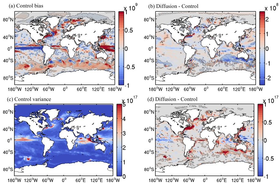
The control integrations without any stochastic perturbations exhibit bias relative to the reanalysis. The daily bias is estimated by taking the difference between the reanalysis and the mean of each ensemble mean over all ten start years. Averaging in time between 60 and 90 days into the integration indicates that this bias, as illustrated for upper 300m ocean heat content in Figure 1(a), often coincides with the regions of high variability such as the eastern tropical Pacific, Southern Ocean, Gulf stream and Kuroshio regions. The upper 300m heat content is chosen as it yields a particularly strong signal to noise ratio compared to sea surface temperatures in isolation.
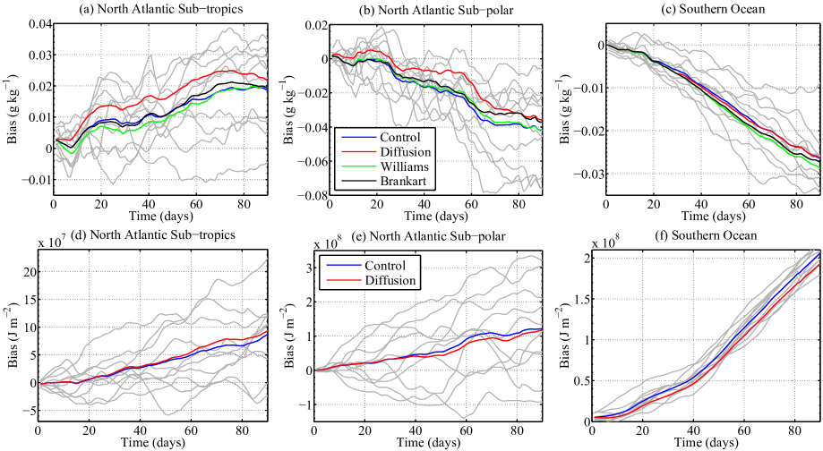
The SPPT scheme leads to a change in the bias in the Southern Ocean, particularly in the region of the south coast of Australia, and the North Atlantic (Figure 1(b)). Comparing panels (a) and (b) in Figure 1 indicates that the warm bias along the south coast of Australia is reduced. Taking the area means, specified in section 2, of the daily bias (Figure 2) highlights a reduction in the mean bias for the upper 300m ocean heat content and sea surface salinity (SSS) in the North Atlantic subpolar region after the first month. The bias is initially not exactly zero due to the random spread in the initial condition perturbations. In the Southern Ocean, while the warm bias has been reduced, no noticeable changes are observed in the SSS bias. In contrast, the bias in the North Atlantic subtropical region has increased due to SPPT. For certains regions the difference in bias remains relatively constant over the length of the integration.
The grey lines in Figure 2 represent the ensemble mean bias of the control integration for each of the 10 years and can be considered as an indicator of confidence. Changes in the ensemble bias and spread (defined as the ensemble variance) between the control and integrations using the SSF and SES schemes are too small to distinguish from zero. The inherent ensemble spread due to the ocean initial condition perturbations and atmospheric variability is large in comparison. When it comes to the area-averaged quantities, Figure 2 also confirms that the SSF and SES schemes have little impact upon the bias though there are regions in which the bias appears slightly reduced (e.g., North Atlantic subpolar SSS around 2-3 months for the SES scheme).
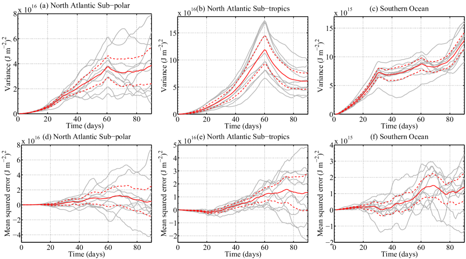
The impact of the SPPT scheme upon the ensemble spread is apparent in several key regions (Figure 1(d)). The largest and most significant impact is shown in the region of the south coast of Australia with patches of visibly increased spread throughout the Southern Ocean. This is a similar pattern to the changes in vertical mixing induced by a stochastic wind forcing compared to climatological wind forcing (Balan Sarojini and von Storch, 2009, compare with their Figure 8). In addition to the Southern Ocean, Figure 1(d) also reveals increased ensemble spread along western boundary currents, including the Gulf stream and Kuroshio. Although there are reductions of ensemble spread in parts of the tropics, they are not distinguishable from zero using the criteria (1). The increase in ensemble spread over the length of the integrations is readily seen in area means of the North Atlantic subtropical and subpolar regions and the Southern Ocean (Figure 3 a-c). The sharp changes in spread apparent in Figure 3 (a), (b) and (c), is due to a new set of random numbers being chosen every 30 days. We expect that substituting the for auto-regressive processes with the equivalent timescales will remove this artefact.
On the other hand, Figure 3 d-f indicates that the SPPT scheme has increased the regional spread at the expense of increased forecast error in the upper ocean heat content in most regions over the length of the integration. The forecast error is defined as the difference between the bias corrected ensemble mean and the reanalysis. Bias corrected means that the daily bias is subtracted from each integration. The mean squared error is then the squared error, averaged over the region of interest. The forecast error is slightly reduced between 2 and 5 weeks in the North Atlantic subtropical region. Comparing figures 3 (a) with (d), (b) with (e) and (c) with (f), indicate that the additional mean squared error is approximately an order of magnitude lower than the increase in spread. The equivalent results for the SSF and SES schemes show that there is little impact upon the total ensemble spread.
Reducing the time between random numbers from 30 days to 1 day resulted in a reduced impact for the SPPT scheme (to the point at which changes are almost indistinguishable from zero) when comparing ensemble bias, spread and mean squared error to those of the control integration. This supports the conventional hypothesis that the impact of the stochastic term is strongly dependent upon its timescale, with longer timescales corresponding to a larger impact. Integrations in which the spatial correlation of the noise is reduced to a degree grid yield only small changes. We would expect that as the correlation length scale is reduced further, there will come a point at which the impact of the random term is strongly reduced (see for example Juricke et al. (2013)). Additional figures were produced (not shown here) demonstrating the reduced impact at these timescales and equivalent plots for the SSF and SES schemes and the impact on the sea surface temperature and salinity.
4 Conclusions
In this study, we test three oceanic stochastic parameterization schemes: Stochastically Perturbed Parametrization Tendency (SPPT), Stochastic Surface Flux (SSF) (Williams, 2012) and a Stochastic Equation of State (SES) (Brankart, 2013). The relatively simple SPPT scheme, which has proved an important element of an ensemble forecast system in numerical weather prediction, injects multiplicative noise into the prognostic equations with an amplitude proportional to the deterministically parametrized tendencies. These three schemes are applied to the ocean component of a state-of-the-art seasonal coupled forecast system and account in part for the uncertainty in sub-grid processes. The model considered here exhibits relatively large oceanic variability compared to a system run at coarser resolution or without an interactive atmosphere. Using such a model, the impact of the SSF and SES schemes was relatively small at the monthly timescales considered, and will likely be more visible through longer timescale integrations. In the case of the SES and SPPT schemes, the amplitude of the stochastic perturbations was limited by model stability.
Results show that compared with the other schemes, SPPT is an effective stochastic parametrization for increasing ensemble spread for variables such as sea-surface temperature and salinity, and upper 300m ocean heat content. The impact of SPPT was found to be particularly marked, and visible above the background variability, in regions of strong eddy activity, such as along western boundary currents in the Gulf Stream and Kuroshio regions, in the North Atlantic sub-polar region and also in parts of the Southern Ocean.
On the other hand, ensemble-mean forecast skill was not improved by the addition of SPPT, except for in the North Atlantic sub-tropics, and for some regions model bias was made worse. The latter does not necessarily imply that SPPT is unrealistic, since the value of many climate model parameters are found by running the model in deterministic mode and estimating the values that fit the observations best. If a stochastic scheme impacts on the model mean state, then such tuning should be performed using the full stochastic model and not a deterministic approximation to it (Palmer, 2012). In addition to tuning the deterministic parameters of the model, the impact of a stochastic parametrization may be tuned by adjusting the decorrelation timescale and spatial distribution of the random perturbations as well as their magnitude. For our particular configurations, changes to the timescale appeared more important than the spatial scale.
The fact that we have not been able to reduce ensemble-mean forecast error, even when the model fields have been bias corrected a-posteriori, suggests that SPPT may be too crude a scheme for ocean models. In the ocean, sub-grid processes are parametrized largely by diffusion and viscosity. The impact of uncertainty in these terms upon the large-scale oceanic circulation, as simulated by SPPT, may not well reflect the uncertainty in the underlying turbulent processes. What this suggests is that a more positive impact than has been found here requires the development of more sophisticated stochastic schemes for unresolved and missing processes.
The development of such stochastic closures should when possible remain consistent with fundamental physical constraints. For example, our initial implementations of a stochastic Gent-McWilliams scheme violated important non-divergent and adiabatic constraints leading to unrealistic upwelling and growing instabilities occurring as soon as the stochastic forcing is increased beyond a certain amplitude. Avenues for future investigations might include a more sophisticated Gent-McWilliams scheme that has a large impact, is stable over long time periods, and remains consistent with the non-divergent and adiabatic constraints of the deterministic scheme. New stochastic schemes should ultimately be guided by observations, however ocean observations are sparse. As a methodology to develop new parametrizations, high-resolution idealised simulations can be substituted as ”truth” (e.g., Berloff, 2005, 2015) and optimally coarse-grained to derive stochastic terms which can for example be decoupled from the background flow (e.g. Cooper and Zanna, 2015). A complementary approach is to implement a PDF-based parametrization, such as Mana and Zanna (2014) who have developed a stochastic parametrization of ocean mesoscale eddies which depends on the temporal tendency of potential vorticity.
Acknowledgements.
This work was funded by UK NERC grant NE/J00586X/1, along with a generous allocation of super-computer resources from ECMWF. AW was partly supported by the EU project SPECS funded by the European Commission Seventh Framework Research Programme under the grant agreement 308378. Thanks go to Peter Düben and Aneesh Subramanian for useful discussions and encouragement during the preparation of this paper and to J.M. Brankart for sharing the code associated with his parametrization. The model data can be obtained by emailing Stephan Juricke, Stephan.Juricke@physics.ox.ac.uk.References
- Balan Sarojini and von Storch (2009) Balan Sarojini, B., and J.-S. von Storch (2009), Effects of fluctuating daily surface fluxes on the time-mean oceanic circulation, Clim. Dynam., 33, 1–18.
- Balmaseda et al. (2013) Balmaseda, M. A., K. Mogensen, and A. T. Weaver (2013), Evaluation of the ECMWF ocean reanalysis system ORAS4, Q.J.R. Meteorol. Soc., 139, 1132–1161.
- Berloff (2005) Berloff, P. S. (2005), Random-forcing model of the mesoscale oceanic eddies, J. Fluid Mech., 529, 71–95.
- Berloff (2015) Berloff, P. S. (2015), Dynamically consistent parameterization of mesoscale eddies. part I: Simple model, Ocean Modelling, 87, 1–19.
- Brankart (2013) Brankart, J. M. (2013), Impact of uncertainties in the horizontal density gradient upon low resolution global ocean modelling, Ocean Modelling, 66, 64–76.
- Brankart et al. (2015) Brankart, J.-M., G. Candille, F. Garnier, C. Calone, A. Melet, P.-A. Bouttier, P. Brasseur, and J. Verron (2015), A generic approach to explicit simulation of uncertainty in the NEMO ocean model, Geoscientific Model Development Discussions, 8(1), 615–643, 10.5194/gmdd-8-615-2015.
- Buizza et al. (1999) Buizza, R., M. Miller, and T. N. Palmer (1999), Stochastic representation of model uncertainties in the ECMWF ensemble prediction system, Quart. J. Roy. Meteor. Soc., 125, 2887–2908.
- Cooper and Zanna (2015) Cooper, F. C., and L. Zanna (2015), Optimisation of an idealised ocean model, stochastic parameterisation of sub-grid eddies, Ocean Modelling, 88, 38–53.
- Dee et al. (2011) Dee, D. P., S. M. Uppala, A. J. Simmons, P. Berrisford, P. Poli, S. Kobayashi, U. Andrae, M. A. Balmaseda, G. Balsamo, P. B. P. Bechtold, A. C. M. Beljaars, L. van de Berg, J. Bidlot, N. Bormann, C. Delsol, R. Dragani, M. Fuentes, A. J. Geer, L. Haimberger, S. B. Healy, H. Hersbach, E. V. Hólm, L. Isaksen, P. Kållberg, M. Köhler, M. Matricardi, A. P. McNally, B. M. Monge-Sanz, J.-J. Morcrette, B.-K. Park, C. Peubey, P. de Rosnay, C. Tavolato, J.-N. Thépaut, and F. Vitart (2011), The ERA-interim reanalysis: configuration and performance of the data assimilation system, Q. J. R. Meteorol. Soc., 137, 553–597.
- Flato et al. (2013) Flato, G., J. Marotzke, B. Abiodun, P. Braconnot, S. Chou, W. Collins, P. Cox, F. Driouech, S. Emori, V. Eyring, C. Forest, P. Gleckler, E. Guilyardi, C. Jakob, V. Kattsov, C. Reason, and M. Rummukainen (2013), Evaluation of Climate Models. In: Climate Change 2013: The Physical Science Basis. Contribution of Working Group I to the Fifth Assessment Report of the Intergovernmental Panel on Climate Change [Stocker, T.F., D. Qin, G.-K. Plattner, M. Tignor, S.K. Allen, J. Boschung, A. Nauels, Y. Xia, V. Bex and P.M. Midgley (eds.)]., Cambridge University Press, Cambridge, United Kingdom and New York, NY, USA.
- Gent and McWilliams (1990) Gent, P. R., and J. C. McWilliams (1990), Isopycnal mixing in ocean circulation models, J. Phys. Oceanogr., 20, 150–155.
- Held and Larichev (1996) Held, I. M., and V. D. Larichev (1996), A scaling theory for horizontally homogeneous, baroclinically unstable flow on a beta plane, J. Atmos. Sci., 53, 946–952.
- Juricke and Jung (2014) Juricke, S., and T. Jung (2014), Influence of stochastic sea ice parametrization on climate and the role of atmosphere-sea ice-ocean interaction, Phil. Trans. R. Soc. A, 372, 20130,283.
- Juricke et al. (2013) Juricke, S., P. Lemke, R. Timmermann, and T. Rackow (2013), Effects of stochastic ice strength perturbation on arctic finite element sea ice modeling., J. Climate, 26, 3785–3802.
- LaCasce (2008) LaCasce, J. H. (2008), Statistics from Lagrangian observations, Prog. Oceanogr., 77, 1–29.
- LaCasce and Ohlmann (2003) LaCasce, J. H., and C. Ohlmann (2003), Relative dispersion at the surface of the Gulf of Mexico, J. Mar. Res., 61, 285–312.
- Large and Yeager (2009) Large, W. G., and S. G. Yeager (2009), The global climatology of an interannually varying air-sea flux data set, Clim. Dynam., 33, 341–364.
- MacLachlan et al. (2014) MacLachlan, C., A. Arribas, K. A. Peterson, A. Maidens, D. Fereday, A. A. Scaife, M. Gordon, M. Vellinga, A. Williams, R. E. Comer, J. Camp, P. Xaviera, and G. Madec (2014), Global seasonal forecast system version 5 GloSea5: a high-resolution seasonal forecast system, Q. J. R. Meteorol. Soc., 10.1002/qj.2396.
- MacLeod et al. (2015) MacLeod, D. A., H. L. Cloke, F. Pappenberger, and A. Weisheimer (2015), Improved seasonal prediction of the hot summer of 2003 over Europe through better representation of uncertainty in the land surface, Q. J. R. Meteorol. Soc.
- Madec and Imbard (1996) Madec, G., and M. Imbard (1996), A global ocean mesh to overcome the North Pole singularity, Clim. Dyn., 12, 381–388.
- Madec and the NEMO team (2008) Madec, G., and the NEMO team (2008), NEMO ocean engine. Note du Pôle de modélisation, France, no. 27, ISSN No 1288-1619, nemo-ocean.eu.
- Madec et al. (1998) Madec, G., P. Delecluse, M. Imbard, and C. Levy (1998), OPA 8.1 Ocean General Circulation Model reference manual, France, no. 11, 91p.
- Mana and Zanna (2014) Mana, P. P., and L. Zanna (2014), Toward a stochastic parameterization of ocean mesoscale eddies, Ocean Modelling, 79(0), 1 – 20.
- Molteni et al. (2011) Molteni, F., T. Stockdale, M. Balmaseda, G. Balsamo, R. Buizza, L. Ferranti, L. Magnusson, K. Mogensen, T. Palmer, and F. Vitart (2011), The new ECMWF seasonal forecast system (System 4), ECMWF Technical Memoranda, 656.
- Mylne et al. (2002) Mylne, K., R. Evans, and R. Clark (2002), Multi-model multi-analysis ensembles in quasi-operational medium-range forecasting, Q. J. R. Meteorol. Soc., 128, 361–384.
- Palmer (2012) Palmer, T. N. (2012), Towards the probabilistic Earth-system simulator: a vision for the future of climate and weather prediction, Quart. J. Roy. Meteor. Soc., 138(665, B), 841–861, 10.1002/qj.1923.
- Palmer et al. (2004) Palmer, T. N., F. J. Doblas-Reyes, R. Hagedorn, A. Alessandri, S. Gualdi, U. Andersen, H. Feddersen, P. Cantelaube, J.-M. Terres, M. Davey, R. Graham, P. Délécluse, A. Lazar, M. Déqué, J.-F. Guérémy, E. Díez, B. Orfila, M. Hoshen, A. P. Morse, N. Keenlyside, M. Latif, E. Maisonnave, P. Rogel, V. Marletto, and M. C. Thomson (2004), Development of a european multimodel ensemble system for seasonal-to-interannual prediction (DEMETER), Bull. Am. Meteorol. Soc., 85, 853–872, 10.1175/BAMS-85-6-853.
- Palmer et al. (2009) Palmer, T. N., R. Buizza, F. Doblas-Reyes, T. Jung, M. Leutbecher, G. Shutts, M. Steinheimer, and A. Weisheimer (2009), Stochastic parametrization and model uncertainty, ECMWF Technical Memoranda, 598.
- Park et al. (2008) Park, Y.-Y., R. Buizza, and M. Leutbecher (2008), TIGGE: preliminary results on comparing and combining ensembles, Q. J. R. Meteorol. Soc., 134, 2029–2050.
- Roeckner et al. (1996) Roeckner, E., K. Arpe, L. Bengtsson, M. Christoph, M. Claussen, L. Dümenil, M. Esch, M. Giorgetta, U. Schlese, and U. Schulzweida (1996), The atmospheric general circulation model ECHAM-4: Model description and simulation of present day climate, Hamburg, Germany.
- Saha et al. (2014) Saha, S., S. Moorthi, X. Wu, J. Wang, S. Nadiga, P. Tripp, D. Behringer, Y.-T. Hou, H. Chuang, M. Iredell, M. Ek, J. Meng, R. Yang, M. P. Mendez, H. van den Dool, Q. Zhang, W. Wang, M. Chen, and E. Becker (2014), The NCEP climate forecast system version 2, J. Climate, 27, 2185–2208.
- Tebaldi and Knutti (2007) Tebaldi, C., and R. Knutti (2007), The use of the multi-model ensemble in probabilistic climate projections, Phil. Trans. R. Soc. A, 365, 2053–2075, 10.1098/rsta.2007.2076.
- Treguier et al. (1997) Treguier, A. M., I. M. Held, and V. D. Larichev (1997), Parameterization of quasigeostrophic eddies in primitive equation ocean models, J. Phys. Oceanogr., 27, 567–580.
- Weisheimer et al. (2009) Weisheimer, A., F. J. Doblas-Reyes, T. N. Palmer, A. Alessandri, A. Arribas, M. Deque, N. Keenlyside, M. MacVean, A. Navarra, and P. Rogel (2009), ENSEMBLES - a new multi-model ensemble for seasonal-to-annual predictions: Skill and progress beyond DEMETER in forecasting tropical Pacific SSTs, Geophys. Res. Lett., 36, L21,711, 10.1029/2009GL040896.
- Weisheimer et al. (2011) Weisheimer, A., T. N. Palmer, and F. J. Doblas-Reyes (2011), Assessment of representations of model uncertainty in monthly and seasonal forecast ensembles, Geophys. Res. Lett., 38, L16,703, 10.1029/2011GL048123.
- Weisheimer et al. (2014) Weisheimer, A., S. Corti, T. Palmer, and F. Vitart (2014), Addressing model error through atmospheric stochastic physical parametrizations: impact on the coupled ECMWF seasonal forecasting system, Phil. Trans. R. Soc. A, 372, 20130,290, 10.1098/rsta.2013.0290.
- Williams (2012) Williams, P. D. (2012), Climatic impacts of stochastic fluctuations in air-sea fluxes, Geophys. Res. Lett., 39, L10,705.