Electromagnetic multipoles - theory issues

Abstract

Some predictions of the Hypercentral Constituent Quark Model for the helicity amplitudes are discussed and compared with data and with the recent analysis of the Mainz group; the role of the pion cloud contribution in explaining the major part of the missing strength at low $Q^{2}$ is emphasized.

1 The hypercentral Constituent Quark Model

In the hypercentral Constituent Quark Model (hCQM) one introduces the hyperspherical coordinates, which are obtained from the standard Jacobi coordinates $\vec{\rho}$ and $\vec{\lambda}$ substituting the absolute values $\rho$ and $\lambda$ by

$$x=\sqrt{{\vec{\rho}}^{2}+{\vec{\lambda}}^{2}}~{}~{},~{}~{}\quad\xi=arctg(\frac{{\rho}}{{\lambda}}),$$ (1)

where $x$ is the hyperradius and $\xi$ the hyperangle. The potential for the three quark system, $V$, is assumed to depend on the hyperradius $x$ only, that is to be hypercentral. It can be considered as a two-body interaction in the hypercentral approximation, which has been shown to be valid specially for the lower energy states [1]. It can also be viewed as a true three-body potential; actually the fundamental gluon interactions, predicted by QCD, lead to three-quark mechanisms. The situation is similar to the flux tube models, where two-body ($\Delta$-shaped) and three-body ($Y$-shaped) interactions are considered.

For a hypercentral potential, in the three-quark wave function one can factor out the angular and hyperangular parts, which are given by the known hyperspherical harmonics [2] and the Schrödinger equation is reduced to a single equation for the hypercentral wave function. Such hypercentral equation can be solved analytically at least in two cases, that is for the h.o. potential and the hypercoulomb one. The two-body h.o. potential turns out to be exactly hypercentral, since $\sum_{i<j}~{}\frac{1}{2}~{}k~{}(\vec{r_{i}}-\vec{r_{j}})^{2}~{}=~{}\frac{3}{2}~{}k~{}x^{2}~{}$. The $SU(6)$ states in the h.o. model are too degenerate with respect to the observed spectrum. The ’hypercoulomb’ potential [1, 3] $V_{hyc}(x)=-\frac{\tau}{x}$ is not confining, however it leads to a power-law behaviour of the proton form factor and of all the transition form factors [4] and it has a perfect degeneracy between the first $0^{+}$ excitated state and the first $1^{-}$ states. The former can be identified with the Roper resonance and the latter with the negative parity resonances. This degeneracy seems to be in agreement with phenomenology but such feature cannot be reproduced in models with only two-body forces, since the excited $L=0$ state, having one more node, lies above the $L=1$ state.

In the hCQM [5] the confining hypercentral potential is assumed to be of the form

$$V(x)=-\frac{\tau}{x}~{}+~{}\alpha x,$$ (2)

A standard hyperfine interaction [6], treated as a perturbation, is added in order to describe the splittings within the $SU(6)$ multiplets. The non strange spectrum is described with $\tau~{}=~{}4.59$ and $\alpha~{}=~{}1.61~{}fm^{-2}$ and the standard strength of the hyperfine interaction needed for the $N-\Delta$ mass difference [6]. The model, keeping fixed these three parameters, has been applied in order to calculate, that is predict, various quantities of interest, namely the photocouplings [7], the transition helicity amplitudes [8], the elastic nucleon form factors [9] and the ratio between the electric and magnetic form factors [10]. In the following the results of this model for the transition helicity amplitudes will be discussed.

The model has been modified in two respects in order to improve the description of the spectrum. First, isospin dependent terms have been added to the spin-spin ones [11]; the second modification is that to use the correct relativistic kinetic energy [12]. The resulting spectrum is considerably improved, in particular the correct ordering of the Roper resonance and the negative parity states is achieved.

2 The helicity amplitudes

The electromagnetic transition amplitudes, $A_{1/2}$ and $A_{3/2}$, are defined as the matrix elements of the transverse electromagnetic interaction, $H_{e.m.}^{t}$, between the nucleon, $N$, and the resonance, $B$, states:

$$\begin{array}[]{rcl}A_{1/2}&=&\langle B,J^{\prime},J^{\prime}_{z}=\frac{1}{2}\ |H_{em}|N,J~{}=~{}\frac{1}{2},J_{z}=-\frac{1}{2}\ \rangle\\ &&\\ A_{3/2}&=&\langle B,J^{\prime},J^{\prime}_{z}=\frac{3}{2}\ |H_{em}|N,J~{}=~{}\frac{1}{2},J_{z}=\frac{1}{2}\ \rangle\\ \end{array}$$ (3)

The baryon states are obtained using the hCQM:

$$V_{3q}=-\frac{\tau}{x}+\alpha x+H_{hyp}$$ (4)

with the parameters fixed in the previous section.

The transverse transition operator is assumed to be

$$H^{t}_{em}~{}=~{}-~{}\sum_{i=1}^{3}~{}\left[\frac{e_{j}}{2m_{j}}~{}(\vec{p_{j}}\cdot\vec{A_{j}}~{}+~{}\vec{A_{j}}\cdot\vec{p_{j}})~{}+~{}2\mu_{j}~{}\vec{s_{j}}\cdot(\vec{\nabla}\times\vec{A_{j}})\right]~{}~{},$$ (5)

where spin-orbit and higher order corrections are neglected [13, 14]. In Eq. 5 $~{}~{}m_{j}$, $e_{j}$, $\vec{s_{j}}$ , $\vec{p_{j}}$ and $\mu_{j}~{}=~{}\frac{ge_{j}}{2m_{j}}$ denote the mass, the electric charge, the spin, the momentum and the magnetic moment of the j-th quark, respectively, and $\vec{A_{j}}~{}=~{}\vec{A_{j}}(\vec{r_{j}})$ is the photon field.

The proton photocouplings of the hCQM [7] have the same overall behaviour of other CQM, probably because all models have the same SU(6) structure in common. In many cases the strength is underestimated and this is a problem for all CQMs.

Taking into account the $Q^{2}-$behaviour of the transition matrix elements, one can calculate the hCQM helicity amplitudes in the Breit frame [8]. The hCQM results for the S11(1535) resonance [8] are given in Fig. 1. The agreement is remarkable, the more so since the hCQM curve has been published three years in advance with respect to the recent TJNAF data [15]. In general the $Q^{2}$ behaviour of the helicity amplitudes is reproduced, except for discrepancies at small $Q^{2}$, especially in the $A_{3/2}$ amplitudes. These discrepancies could be ascribed either to the non-relativistic character of the model or to the lack of explicit quark-antiquark configurations, which may be important at low $Q^{2}$ . However, the kinematical relativistic corrections at the level of boosting the nucleon and the resonances states to a common frame are not responsible for these discrepancies, as it has been demonstrated in Ref.[16].

Figure 1: Comparison between the experimental data [17, 15] for the helicity amplitude $A^{p}_{1/2}$ of the $S_{11}(1535)$ resonance and the calculations with the hCQM, lower curve [8] also compared with the Capstick and Keister result, upper curve [18].

Keeping fixed the parameters, the hCQM has also been applied to the calculation of the longitudinal helicity amplitudes [19]. An interesting feature is that many amplitudes vanish in the $SU(6)$ limit, therefore a detailed study of the longitudinal strength may be a good test of the $SU(6)$ breaking mechanisms.

It should be mentioned that the r.m.s. radius of the proton corresponding to the parameters of Eq.4 is $0.48~{}fm$, which is just the value fitted in [13] to the $D13$ photocoupling. Therefore the missing strength at low $Q^{2}$ can be ascribed to the outer region of the nucleon, where the lack of quark-antiquark effects are probably important. This view is enforced by a recent analysis [20, 21], which compares the results of the hCQM for the helicity amplitudes and the calculation of the pion cloud contributions performed with the dynamical model of the Mainz Group. As an example, the $A_{3/2}$ for the $N-\Delta$ transition is shown in Fig. 2. The pion cloud turns out to be important at low $Q^{2}$ and diminishes strongly up to $3GeV^{2}$; it accounts for the major part of the discrepancy between the data and the hCQM results. Particularly important is the longitudinal $\Delta$ transition, where the very small hCQM values are compensated by the dominant pion contribution (see [20]).

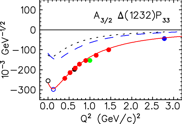
Figure 2: The $Q^{2}$ dependence of the $N\rightarrow\Delta$ $A_{3/2}$ helicity amplitude. The solid curve is the result of the superglobal fit with MAID [22], the data points at finite $Q^{2}$ are obtained with single-Q² fits [21]. The dashed and dotted curves are, respectively, the predictions of the hyperspherical constituent quark model [8] and the pion cloud contributions calculated with DMT by the Mainz group [23]. At $Q^{2}=0$ the photon coupling from PDG is shown [24].

References

- [1] M. Fabre de la Ripelle and J. Navarro, Ann. Phys. (N.Y.) 123, 185 (1979).
- [2] J. Ballot and M. Fabre de la Ripelle, Ann. of Phys. (N.Y.) 127, 62 (1980).
- [3] E. Santopinto, M.M. Giannini and F. Iachello, in ”Symmetries in Science VII”, ed. B. Gruber, Plenum Press, New York, 445 (1995); F. Iachello, in ”Symmetries in Science VII”, ed. B. Gruber, Plenum Press, New York, 213 (1995).
- [4] E. Santopinto, F. Iachello and M.M. Giannini, Nucl. Phys. A623, 100c (1997).
- [5] M. Ferraris, M.M. Giannini, M. Pizzo, E. Santopinto and L. Tiator, Phys. Lett. B364, 231 (1995).
- [6] N. Isgur and G. Karl, Phys. Rev. D18, 4187 (1978); Phys. Rev. D19, 2653 (1979).
- [7] M. Aiello, M. Ferraris, M.M. Giannini, M. Pizzo and E. Santopinto, Phys. Lett. B387, 215 (1996).
- [8] M. Aiello, M. M. Giannini, E. Santopinto, J. Phys. G: Nucl. Part. Phys. 24, 753 (1998)
- [9] M. De Sanctis, E. Santopinto, M.M. Giannini, Eur. Phys. J. A1, 187 (1998).
- [10] M. De Sanctis et al., Phys. Rev. C62,025208 (2000).
- [11] M.M. Giannini, E. Santopinto, A. Vassallo, Eur. Phys. J. A12, 447 (2001).
- [12] M.M. Giannini, E. Santopinto, A. Vassallo, to be published.
- [13] L. A. Copley, G. Karl and E. Obryk, Phys. Lett. 29, 117 (1969).
- [14] R. Koniuk and N. Isgur, Phys. Rev. D21, 1868 (1980).
- [15] R.A. Thompson et al., Phys. Rev. Lett. 86, 1702 (2001).
- [16] M. De Sanctis, E. Santopinto, M.M. Giannini, Eur. Phys. J. A2, 403 (1998).
- [17] V. D. Burkert,arXiv:hep-ph/0207149.
- [18] S. Capstick and B.D. Keister, Phys. Rev.D 51, 3598 (1995).
- [19] M.M. Giannini and E. Santopinto, to be published.
- [20] L. Tiator, Contribution to the Brag Meeting, these Proceedings.
- [21] L. Tiator et al., Eur. Phys. J. A19 (Suppl. 1), 55 (2004).
- [22] D. Drechsel et al., Nucl. Phys. A645 (1999) 145; http://www.kph.uni-mainz.de/MAID.
- [23] S. Kamalov et al., Phys. Rev. C 64 (2001) 032201; http://www.kph.uni-mainz.de/MAID/dmt/.
- [24] K. Hagiwara et al. (Particle Data Group), Phys. Rev. D 66 (2002) 010001.