Small-amplitude swimmers can self-propel faster in viscoelastic fluids

Abstract

Many small organisms self-propel in viscous fluids using travelling wave-like deformation of their bodies or appendages. Examples include small nematodes moving through soil using whole-body undulations or spermatozoa swimming through mucus using flagellar waves. When self-propulsion occurs in a non-Newtonian fluid, one fundamental question is whether locomotion will occur faster or slower than in a Newtonian environment. Here we consider the general problem of swimming using small-amplitude periodic waves in a viscoelastic fluid described by the classical Oldroyd-B constitutive relationship. Using Taylor’s swimming sheet model, we show that if all travelling waves move in the same direction, the locomotion speed of the organism is systematically decreased. However, if we allow waves to travel in two opposite directions, we show that this can lead to enhancement of the swimming speed, which is physically interpreted as due to asymmetric viscoelastic damping of waves with different frequencies. A change of the swimming direction is also possible. By analysing in detail the cases of swimming using two or three travelling waves, we demonstrate that swimming can be enhanced in a viscoelastic fluid for all Deborah numbers below a critical value or, for three waves or more, only for a finite, non-zero range of Deborah numbers, in which case a finite amount of elasticity in the fluid is required to increase the swimming speed.

I Introduction

A variety of small prokaryotic and eukaryotic organisms exploit viscous forces from a surrounding fluid in order to self propel. The low Reynolds number at which they swim means there are no inertial effects, and work must be constantly expanded by the cells to produce motion. This is achieved, for example, by the rotation of rigid helical appendages Purcell1997 or by the propagation of planar travelling waves along a flexible flagellum Winet1977 . Our fundamental understanding of swimming cells has increased dramatically with the advancement of imaging techniques and computer power for more realistic numerical simulations Powers2009 .

The vast majority of work on swimming at low Reynolds number has focused on swimmers moving in Newtonian fluids. However, in vivo, many self-propelled organisms progress through non-Newtonian fluids. Examples include the motion of cilia in lung mucus Liron1988 , nematodes travelling though soil Wallace1967 , bacteria in their host’s tissue Suerbaum2002 , and spermatozoa swimming though cervical mammalian mucus Pacey2006 . An important question is how a transition from a Newtonian to a non-Newtonian fluid affects the dynamics and kinematics of micro-swimmers. In this paper, we use a simplified modelling approach to quantify whether non-Newtonian stresses can help the micro-swimmers go faster or if they hinder their motion, and how this affects their mechanical efficiency.

Experimental studies have not yet reached a clear consensus on whether viscoelasticity increases or decreases swimming velocities. Instead a range of results has been reported for different kinematics and rheological properties. Nematodes swimming in concentrated solutions of rod-like polymers undergo an increase in swimming speed Arratia2013 . In that case, the polymers, aligned by the stress caused by the nematode, form local nematic structures which give rise to shear-thinning and aid the forward propulsion of the nematode. In contrast, solutions of long flexible polymers with no shear-thinning but strong elasticity lead to a decrease of the nematode’s swimming speed Arratia2011 . An experiment imitating Taylor’s classic swimming sheet Taylor1951 in rotational (planar) geometry shows exactly opposite effects with an increased locomotion in a Boger (constant-viscosity, elastic) fluid but a decrease in a shear-thinning fluid Kudrolli2013 . Recently, the locomotion of flexible-tailed swimmers was also shown to be enhanced in a Boger fluid Zenit2013 .

Previous theoretical studies addressing motion in complex fluids have considered a variety of kinematics, including undulatory motion Lauga2007 ; Loghin2013 , helical rotation Wolgemuth2007 , squirming Brandt2011 ; laipof1 , three-sphere models Gaffney2013 , and paddlers Loghin2013 . Methods that are ineffectual in a Newtonian fluid due to reversibility Purcell1977 , such as flapping Lauga2008 or solid body rotation pak12 , can also be exploited in a non-Newtonian setting to induce propulsion lauga_life ; Lauga2011 . In the case of locomotion using helical flagella, small-amplitude helices always go slower, but for larger amplitudes, a modest increase is possible liu2011 . In this paper, we focus on planar wave motion, a situation for which there is a wealth of work starting with Taylor’s swimming sheet Taylor1951 . In the presence of a surrounding elastic structure, non-Newtonian stresses were shown computationally to lead to faster and more efficient swimming Shelley2013 . Numerical simulations also demonstrated that for high-amplitude motion, both shear-thinning Loghin2013 and polymeric Oldroyd-B fluids Shelley2010 ; spagnolie2013 ; Thomases2014 could lead to faster locomotion. In particular, using simulations on finite swimming sheets it has been shown that front-back stress asymmetry together with swimmer flexibility leads to increased swimming speeds Thomases2014 .

Analytical work on locomotion by waving focuses on small-amplitude motion. In the case of isolated swimmers, enhanced swimming was predicted theoretically to take place in gels Powers2010 , Brinkmann fluids Leshansky2009 and – with the addition of elastohydrodynamic effects – viscoelastic fluids Riley2014 , but not in inelastic shear-thinning fluids velezcordero13 . Two nearby swimmers also synchronise faster in an elastic fluid than in a Newtonian medium Elfring2010 . However, in the case of polymeric fluids, asymptotic results predicted a systematic decrease of the swimming speed for all constitutive models, including all Oldroyd-like fluids Lauga2007 and general linear viscoelastic fluid models Powell1998 in the case of prescribed waveform swimming. A decrease also takes place in the case of helical small-amplitude motion Wolgemuth2007 ; FuWolgemuthPowers2009 . Provided the prescribed waving amplitude is small compared to its wavelength, it appears thus that an isolated swimmer is always slowed down by viscoelastic stresses.

In this paper, we consider mathematically the most general problem for planar locomotion using small-amplitude waves periodic both in space and in time. Specifically, we prescribe the shape deformation as a sum of waves travelling with different wavenumbers and frequencies and in different directions and consider the resulting locomotion in a viscoelastic, Oldroyd-B fluid. We show that swimming in a non-Newtonian fluid at small amplitudes need not always lead to slower swimming compared to the Newtonian case, provided the right combination of waves are considered. For swimming enhancement to be observed, different waves need to travel in opposite directions, and the enhancement in that case results from the asymmetric viscoelastic damping of waves with different frequencies. A change of the swimming direction is also possible. After presenting the general derivations, and introducing a sufficient condition for enhanced locomotion, we analyse in detail the cases of two or three travelling waves. The enhancement in a viscoelastic fluid can be obtained for all Deborah numbers below a critical value or, in the case of three waves or more, only if a finite amount of elasticity is present in the fluid.

II General small-amplitude wave in a viscoelastic Fluid

II.1 Setup

Analogous to Taylor’s classic swimming calculation Taylor1951 ; Lauga2007 , an infinite inextensible sheet of negligible thickness is placed in a fluid and undergoes waving motion. The waveform of the sheet is prescribed, and results in swimming. In the frame of the swimmer the oscillation of the vertical position, $y(x,t)$, of the sheet is described by

$$y(x,t)=b\sum\limits_{n=-\infty}^{+\infty}\sum\limits_{m=-\infty}^{+\infty}\alpha_{n,m}e^{i(mkx-n\omega t)},$$ (1)

where $x$ denotes the coordinate along the average sheet axis and $t$ time. In Eq. (1) the modes $n=0$ and $m=0$ are omitted as there is no mean deformation in $x$ or in time. The fluid is assumed to be located above the sheet along the $y>0$ direction In Eq. (1), $b$ is the sheet amplitude, $k$ the fundamental wavelength and $\omega$ the fundamental frequency. We allow both positive and negative values of the mode number $(m,n)$ in order to include waves travelling in both directions along the sheet. The order-one complex coefficients $\alpha_{n,m}$ represent dimensionless Fourier amplitude of each $(m,n)$ mode and since $y$ is real they satisfy $\alpha_{-n,-m}=\alpha_{n,m}^{*}$. To simplify notation all sums over $n$ and $m$ from $-\infty$ to $+\infty$ will be denoted with a single summation symbol, $\sum_{n,m}$.

Upon non-dimensionalising $x$ by $k^{-1}$ and $t$ by $\omega^{-1}$, Eq. (1) becomes

$$y(x,t)=\epsilon\sum\limits_{n,m}\alpha_{n,m}e^{i(mx-nt)},$$ (2)

with a prefactor $\epsilon=bk$ defined as the ratio of the sheet amplitude to its wavelength. We assume that this ratio is small in this paper, $\epsilon\ll 1$, allowing the swimming speed to be computed as an asymptotic expansion in $\epsilon$.

As the sheet is infinite along the $z$ direction we can reduce the three-dimensional swimming problem to two dimensions. The velocity field is written as $\mathbf{u}=u_{x}\mathbf{e}_{x}+u_{y}\mathbf{e}_{y}$. This allows a streamfunction, $\psi(x,y,t)$, to be defined such that $u_{x}=\partial\psi/\partial y$ and $u_{y}=-\partial\psi/\partial x$, ensuring that the flow remains incompressible.

In order to find the streamfunction we must first consider the boundary conditions imposed on the flow. On the waving sheet the no slip boundary condition enforces the velocity of the fluid at the sheet location to be the same as the velocity of the sheet, so that

$$\nabla\psi|_{x,y(x,t)}=\epsilon\sum\limits_{n,m}in\alpha_{n,m}e^{i(mx-nt)}\mathbf{e}_{x}.$$ (3)

Far away from the sheet we expect that the flow will be unaffected by the wavemotion. Hence in the frame of the swimmer, the far field velocity will be the speed of the swimmer, but in the opposite direction. So if the steady swimming of the sheet is denoted $-U\mathbf{e}_{x}$ then we have the boundary condition

$$\nabla\psi|_{x,\infty}=U\mathbf{e}_{y},$$ (4)

where the value of $U$ is to be determined.

II.2 Constitutive relationship: Oldroyd-B fluid

The swimmer is self-propelling in a fluid described by the Oldroyd-B constitutive relationship, modelling a dilute solution of infinitely extensible polymers in a Newtonian solute as a homogeneous continuum Oldroyd1950 ; Phanbook . In this classical model, the shear viscosity is constant but the polymer elasticity affects the flow, giving rise to normal stresses. This is a good model for the Boger fluids used in many non-Newtonian micro-swimmer experiments Phanbook . Furthermore, from Ref. Lauga2007 , we expect that to second order in $\epsilon$, our asymptotic results will remain valid for a large class of constitutive relationships.

If $p$ denotes the pressure and $\boldsymbol{\tau}$ the deviatoric stress, Cauchy’s equation of mechanical equilibrium in the absence of inertia is simply written

$$\nabla p=\bf\nabla\cdot\boldsymbol{\tau}.$$ (5)

In an Oldroyd-B fluid, the total deviatoric stress, $\boldsymbol{\tau}$, a combination of stresses from the Newtonian solvent $\boldsymbol{\tau}_{s}$, and those from the polymers $\boldsymbol{\tau}_{p}$, is written as $\boldsymbol{\tau}=\boldsymbol{\tau}_{s}+\boldsymbol{\tau}_{p}$. If $\eta_{s}$ denotes the solvent viscosity and assuming that $\boldsymbol{\tau}_{p}$ follows a first-order Maxwell constitutive equation with relaxation time $\lambda$, elastic modulus $G$, and polymer viscosity $\eta_{p}=G/\lambda$, the total stress obeys Phanbook

$$\boldsymbol{\tau}+\lambda\stackrel{{\scriptstyle\triangledown}}{{\boldsymbol{\tau}}}=\eta\dot{\boldsymbol{\gamma}}+\eta_{s}\lambda\stackrel{{\scriptstyle\triangledown}}{{\dot{\boldsymbol{\gamma}}}},$$ (6)

where $\dot{\boldsymbol{\gamma}}$ is the shear rate tensor, defined as $\dot{\boldsymbol{\gamma}}=\nabla{\bf u}+\nabla{\bf u}^{T}$, and $\eta=\eta_{s}+\eta_{p}$ is the sum of the solvent and polymer viscosities. In Eq. (6), the upper-convected derivative defines the rate of change of the tensor $\bf A$ while it translates and deforms with the fluid and is written as

$$\stackrel{{\scriptstyle\triangledown}}{{{\bf A}}}=\frac{\partial{\bf A}}{\partial t}+\mathbf{u}\cdot\nabla{\bf A}-(\nabla\mathbf{u}^{T}\cdot{\bf A}+{\bf A}\cdot\nabla\mathbf{u}).$$ (7)

Upon non-dimensionalising stresses by $\eta\omega$ and shear rates by $\omega$, Eq. (6) becomes

$$\boldsymbol{\tau}+{\rm De}\stackrel{{\scriptstyle\triangledown}}{{\boldsymbol{\tau}}}=\dot{\boldsymbol{\gamma}}+\beta{\rm De}\stackrel{{\scriptstyle\triangledown}}{{\dot{\boldsymbol{\gamma}}}},$$ (8)

where $\beta=\eta_{s}/\eta\leq 1$, and ${\rm De}=\lambda\omega$ is the Deborah number that describes the relative importance of viscoelasticity by comparing the relaxation time to the timescale on which the fluid is perturbed, given by $1/\omega$, where $\omega$ is the fundamental waving frequency.

II.3 Asymptotic solution

Since we have $\epsilon\ll 1$ we seek to find solutions to the stress, streamfunction and velocity in terms of perturbative expansion in $\epsilon$, such that

$$\psi=\epsilon\psi_{1}+\epsilon^{2}\psi_{2}+\dots,$$ (9)

$$\boldsymbol{\tau}=\epsilon\boldsymbol{\tau}_{1}+\epsilon^{2}\boldsymbol{\tau}_{2}+\dots,$$ (10)

$$U=\epsilon^{2}U_{2NN}+\dots.$$ (11)

The swimming velocity is expected to be quadratic in $\epsilon$, and so we focus on the first and second-order solutions (the subscript $NN$ is used as a reminder that the final result for the swimming speed will quantify non-Newtonian swimming).

II.3.1 Solution at order $\epsilon$

The leading-order constitutive equation is linear and given by

$$\boldsymbol{\tau}_{1}+{\rm De}\frac{\partial\boldsymbol{\tau}_{1}}{\partial t}=\dot{\boldsymbol{\gamma}}_{1}+\beta{\rm De}\frac{\partial\dot{\boldsymbol{\gamma}}_{1}}{\partial t}\cdot$$ (12)

This can be reduced into a streamfunction equation by taking its divergence, combining with Eq. (5), and taking the curl to eliminate the pressure, leaving

$$\left(1+\beta{\rm De}\frac{\partial}{\partial t}\right)\nabla^{4}\psi_{1}=0.$$ (13)

The post-transient solution to Eq. (12) is found using Fourier notation and solving the biharmonic equation analytically, leading to

$$\psi_{1}=\sum\limits_{n,m}\alpha_{n,m}\frac{n}{m}(1+|m|y)e^{-|m|y}e^{i(mx-nt)},$$ (14)

where the first-order boundary conditions,

$$\nabla\psi_{1}|_{x,0}=\sum\limits_{n,m}in\alpha_{n,m}e^{i(mx-nt)}\mathbf{e}_{x},$$ (15a)

and

$$\nabla\psi_{1}|_{x,\infty}=\mathbf{0},$$ (15b)

are satisfied. Clearly, the first-order solution is the same as the Newtonian case, and as expected there is no swimming at this order.

II.3.2 Solution at order $\epsilon^{2}$

At order $\epsilon^{2}$, the constitutive equation, Eq. (8), is given by

$$\left(1+{\rm De}\frac{\partial}{\partial t}\right)\boldsymbol{\tau}_{2} -\left(1+\beta{\rm De}\frac{\partial}{\partial t}\right)\dot{\boldsymbol{\gamma}}_{2}=$$

$${\rm De}(\nabla\mathbf{u}_{1}^{T}\cdot\boldsymbol{\tau}_{1}+\boldsymbol{\tau}_{1}\cdot\nabla\mathbf{u}_{1}-\mathbf{u}_{1}\cdot\nabla\boldsymbol{\tau}_{1})$$

$$-\beta{\rm De}(\nabla\mathbf{u}^{T}_{1}\cdot\dot{\boldsymbol{\gamma}}+\dot{\boldsymbol{\gamma}}\cdot\nabla\mathbf{u}_{1}-\mathbf{u}\cdot\nabla\dot{\boldsymbol{\gamma}}_{1}).$$ (16)

Using Fourier notation of the form

$$\mathbf{A}=\sum\limits_{n,m}\tilde{\mathbf{a}}^{(n,m)}e^{-int},$$ (17)

for any tensor, vector, or scalar, the first-order constitutive equation, Eq. (12), gives access to the Fourier component of the first-order stress as

$$\tilde{\boldsymbol{\tau}}_{1}^{(n,m)}=\frac{1-in\beta{\rm De}}{1-in{\rm De}}\tilde{\dot{\boldsymbol{\gamma}}}_{1}^{(n,m)}.$$ (18)

As we are interested in the time-averaged swimming, it is sufficient to focus on the time-averaged version of Eq. (16). We then use Eq. (18) to express the mean of Eq. (16) using the Fourier modes of its right-hand-side, and obtain

$$\langle\boldsymbol{\tau}_{2}\rangle-\langle\dot{\boldsymbol{\gamma}}_{2}\rangle= \sum\limits_{n,m}\frac{{\rm De}(1-\beta)}{1-in{\rm De}}\times$$

$$(\nabla\mathbf{u}_{1}^{T\ast}\cdot\dot{\boldsymbol{\gamma}}+\dot{\boldsymbol{\gamma}}\cdot\nabla\mathbf{u}_{1}^{\ast}-\mathbf{u}_{1}^{\ast}\cdot\nabla\dot{\boldsymbol{\gamma}})^{(n,m)}.$$ (19)

With the first-order streamfunction whose Fourier component is

$$\tilde{\psi}_{1}^{(n,m)}=\alpha_{n,m}\frac{n}{m}(1+|m|y)e^{-|m|y}e^{imx},$$ (20)

we obtain the Fourier modes of the flow velocity,

$$\tilde{\mathbf{u}}_{1}^{(n,m)}=\alpha_{n,m}\frac{n}{m}e^{-|m|y}e^{imx}\left(\begin{array}[]{c}-|m|^{2}y\\ -(1+|m|y)im\end{array}\right),$$ (21)

the velocity gradient,

$$\nabla\tilde{\mathbf{u}}_{1}^{(n,m)}= \,\alpha_{n,m}\frac{n}{m}e^{-|m|y}e^{imx}\times$$

$$\left(\begin{array}[]{cc}-im|m|^{2}y&m^{2}(1+|m|y)\\ |m|^{3}y-|m|^{2}&im|m|^{2}y\end{array}\right),$$ (24)

and the shear stress tensor,

$$\tilde{\dot{\boldsymbol{\gamma}}}_{1}^{(n,m)}=\alpha_{n,m}\frac{n}{m}e^{-|m|y}e^{imx}\left(\begin{array}[]{cc}-2im|m|^{2}y&2|m|^{3}y\\ 2|m|^{3}y&2im|m|^{2}y\end{array}\right).$$ (25)

The divergence and curl are then taken, as before, to obtain an explicit equation for the second-order streamfunction as

$$\frac{d^{4}\langle\psi_{2}\rangle}{dy^{4}}=\sum\limits_{n,m}-|\alpha_{n,m}|^{2}\frac{n^{2}}{m^{2}}\frac{(\beta-1){\rm De}}{1-in{\rm De}}\times$$

$$\,\,\frac{{\rm d}^{2}}{{\rm d}y^{2}}\Big{[}e^{-2|m|y}\left(-4im|m|^{4}y+4im|m|^{5}y^{2}-2|m|^{3}im\right)\Big{]}.$$ (26)

Integrating with respect to $y$ three times, this gives

$$\frac{{\rm d}\langle\psi_{2}\rangle}{{\rm d}y}=Ay^{2}+By+C+$$

$$\sum\limits_{n,m}|\alpha_{n,m}|^{2}\frac{n^{2}}{m^{2}}\frac{(\beta-1){\rm De}}{1-in{\rm De}}e^{-2|m|y}(-2im|m|^{4}y^{2}+im|m|^{2}).$$ (27)

Given the form of the boundary conditions at infinity, Eq. (4), we obtain $A=B=0$ and $C$ is equal to the second-order swimming speed, hence $C=U_{2NN}$. Its value can be found using the time-averaged second-order boundary condition,

$$\frac{{\rm d}\langle\psi_{2}\rangle}{{\rm d}y}\Big{|}_{x,0}=\sum\limits_{n,m}nm|\alpha_{n,m}|^{2},$$ (28)

leading to

$$U_{2NN}=\sum\limits_{n,m}nm|\alpha_{n,m}|^{2}\left(\frac{1-in{\rm De}\beta}{1-in{\rm De}}\right).$$ (29)

Rewriting Eq. (29) with sums in $n$ and $m$ running from $1$ to $\infty$ only, and using that $\alpha_{-n,-m}=\alpha_{n,m}^{*}$, leads to a simplified expression for the final result as

$$U_{2NN}=2\sum\limits_{n\geq 1}\sum\limits_{m\geq 1}nm(|\alpha_{n,m}|^{2}-|\alpha_{n,-m}|^{2})\left(\frac{1+\beta n^{2}{\rm De}^{2}}{1+n^{2}{\rm De}^{2}}\right),$$ (30)

where the opposite-sign contributions of waves travelling in the $+x$ and $-x$ direction are apparent.

III A sufficient condition for enhanced swimming

The result in Eq. (30) gives the leading-order swimming speed of the swimming sheet with the most general shape deformation periodic in both $x$ and $t$. When there are no viscoelastic effects ${\rm De}=0$, and the Newtonian result is recovered. We denote the swimming speed $U_{2N}$ in that case.

As can be seen in Eq. (30), it is the value of the (dimensionless) frequency $n$ that affects the non-Newtonian change of each mode, not the value of the (dimensionless) wavenumber $m$. In order to gain insight into the conditions for swimming to be enhanced or slowed down by the presence of viscoelastic stresses, let us focus on the simple case where only the modes $|m|=|n|$ are present. The sheet deformation is written now as a linear superposition of travelling waves

$$y=\epsilon\sum\limits_{n\geq 1}\alpha_{+n}e^{in(x-t)}+\alpha_{-n}e^{in(x+t)},$$ (31)

where $\alpha_{+n}$ and $\alpha_{-n}$ describes the $n$th mode wave travelling to the right ($x>0$) and left ($x<0$) respectively. Using Eq. (30) this leads to non-Newtonian swimming with speed

$$U_{2NN}=\sum\limits_{n\geq 1}a_{n}\left(\frac{1+n^{2}\beta{\rm De}^{2}}{1+n^{2}{\rm De}^{2}}\right),$$ (32)

and Newtonian swimming with speed,

$$U_{2N}=\sum\limits_{n\geq 1}a_{n},$$ (33)

where, we have further simplified notation such that

$$a_{n}=2n^{2}(|\alpha_{+n}|^{2}-|\alpha_{-n}|^{2}),$$ (34)

describes the superposition of mode $n$ waves in both directions. Clearly, for both Newtonian and non-Newtonian cases, the addition of backwards waves always reduces the absolute value of the swimming speed. Let us now focus on the relative change in speed when comparing swimming between a Newtonian and a non-Newtonian fluid.

Using only inspection we cannot, a priori, define a range of Deborah number where we expect to see an increase in speed from the Newtonian to the non-Newtonian swimming (i.e. $U_{2NN}/U_{2N}>1$). In order to look for further insight, we consider the infinite and zero Deborah number limits. At zero Deborah number, where there are no elastic effects, the ratio of swimming speeds is equal to 1. In the limit of large Deborah numbers ${\rm De}\gg 1$, where elastic effects dominate, it is straightforward to get from Eq. (32) that $U_{2NN}/U_{2N}=\beta<1$, and thus swimming is always eventually decreased. As the value of ${\rm De}$ increases from zero to infinity, the speed ratio could monotonically decrease from $1$ to $\beta$, in which case no enhancement would be seen, or non-monotonically, where enhancement could take place.

Our numerical simulations indicate that in the cases where the speed ratio does go above 1, then in most cases it is always increasing in the neighbourhood of ${\rm De}=0$ before monotonically decreasing to $\beta$ (see numerical results in Fig. 1 and discussion below). In order to characterise the behavior around ${\rm De}=0$, we can compute derivatives and Taylor-expand the ratio of swimming speeds. The first derivative ${\partial U_{2NN}}/{\partial{\rm De}}$ evaluated at ${\rm De}=0$ is zero because the swimming speed depends quadratically on the Deborah number. However, the second derivative (the curvature) is non-zero, and is given by

$$\frac{\partial^{2}U_{2NN}}{\partial{\rm De}^{2}}\bigg{|}_{{\rm De}=0}=\sum\limits_{n\geq 1}2n^{2}a_{n}(\beta-1).$$ (35)

When it is divided by the Newtonian swimming speed, Eq. (33), the above gives access to the curvature of $U_{2NN}/U_{2N}$ at ${\rm De}=0$ (this is equivalent to taking the first derivative of the speed ratio with respect to ${\rm De}^{2}$). If that curvature is positive, then faster swimming occurs in the neighbourhood of ${\rm De}=0$. As we always have $\beta<1$, the curvature is positive if there is a sign difference between the sums in Eqs. (33)-(35) and therefore a sufficient condition for enhanced swimming is the kinematic condition

$$\left[\sum\limits_{n\geq 1}a_{n}\right]\times\left[\sum\limits_{n\geq 1}n^{2}a_{n}\right]<0.$$ (36)

In order to achieve the condition in Eq. (36), waves travelling in opposite directions are required. Indeed, for example if all $a_{n}$ amplitudes are positive, then it is easy to see from Eq. (32) that each $a_{n}$ mode decreases in amplitude, resulting in an overall decrease in magnitude of the speed. If there are waves travelling in both direction, i.e. at least one $\alpha_{-n}\neq 0$ and one $\alpha_{+n}\neq 0$, then they need different combinations of amplitudes and frequencies in order to satisfy the condition in Eq. (36). Hence a combination of positive and negative $a_{n}$ values are required.

Physically, the increase in swimming speed between Newtonian and viscoelastic fluids seen here arises from the fact that the damping caused by a non-zero Deborah number affects modes with different frequencies differently. Specifically, the damping term of the form $({1+n^{2}\beta{\rm De}^{2}})/({1+n^{2}{\rm De}^{2}})$ decreases monotonically with $n$. Modes with higher frequencies are therefore damped more than those with lower values of $n$, which provides a mechanism for enhanced swimming.

For illustration, consider two waves travelling in opposite directions with the high-frequency ($n$) wave travelling along the $-x$ direction ($a_{n}<0$) and the low-frequency ($m$) one along the $+x$ direction ($a_{m}>0$). Then their respective amplitudes be such that the resulting Newtonian swimming speed is positive, $U_{2N}>0$. In the viscoelastic fluid, the $a_{n}$ wave will be damped more than the $a_{m}$ wave, as $n>m$. On one hand, decreasing the magnitude of the $a_{n}$ wave will increase the swimming speed while on the other hand, decreasing the $a_{m}$ mode will hinder the swimming velocity – it is thus a matter of relative decrease. If the wave amplitudes are such that the gain found by suppressing the $a_{n}$ wave more than compensates for the damping of the $a_{m}$ wave, then the non-Newtonian swimming speed will be above the Newtonian one, $U_{2NN}>U_{2N}$. If the wave amplitudes are such that $U_{2N}<0$, then a similar reasoning might be used to lead to $U_{2NN}>0$ and in that case, viscoelasticity might lead to a reversal of the direction of locomotion.

IV Superposition of two travelling waves: continuous enhancement

We now consider in detail simple cases. We start by swimming using two travelling waves, and show that in this case the sufficient condition described above is in fact necessary: when enhancement takes place, it will lead to faster swimming for all Deborah numbers below a critical value. In order to analytically describe situations where faster swimming can occur, two simple waveforms each containing two waves travelling in opposite directions will be considered. Clearly these two travelling waves must have different frequencies, otherwise they are both damped in the same proportion by viscoelasticity and the swimming speed decreases.

IV.1 Superposition of two travelling waves with identical wave speeds

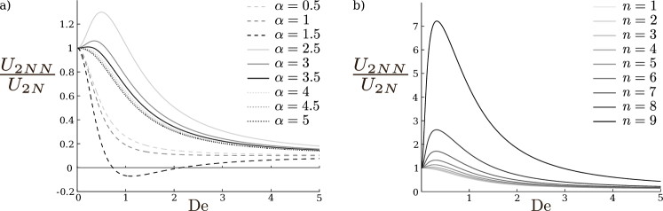
Figure 1: Ratio between the non-Newtonian swimming speed $U_{2NN}$, and the Newtonian value $U_{2N}$, as a function of the Deborah number, ${\rm De}$, for various values of the relative wave amplitude $\alpha$, and frequency ratio $n$, in the waveform from Eq. (37). Here we have chosen $\beta=0.1$. Left: fixed value of $n=2$ and a range of $\alpha$ values (between 0.5 and 5). Right: fixed value of $\alpha=9.5$ and $n$ ranging between $n=1$ and $9$.

An example of two waves with different frequencies modes, amplitudes, and wave direction but identical magnitude of wave speed is given by

$$y(x,t)=\epsilon\left[\alpha\sin(x-t)+\sin n(x+t)\right],$$ (37)

where $\alpha$ is the dimensionless ratio of amplitudes between the two waves. Using Eqs. (32) and  (33) for the sinusoidal waveform in Eq. (37) we get the second-order Newtonian swimming speed as

$$U_{2N}=\frac{1}{2}(\alpha^{2}-n^{2}),$$ (38)

while the second-order non-Newtonian swimming speed is given by

$$U_{2NN}=\frac{\alpha^{2}}{2}\bigg{(}\frac{1+\beta{\rm De}^{2}}{1+{\rm De}^{2}}\bigg{)}-\frac{n^{2}}{2}\bigg{(}\frac{1+n^{2}\beta{\rm De}^{2}}{1+n^{2}{\rm De}^{2}}\bigg{)}.$$ (39)

To find where faster swimming occurs, we compute as above the second derivative of the swimming ratio, $U_{2NN}/U_{2N}$ with respect to ${\rm De}$ at ${\rm De}=0$, giving

$$\frac{\partial^{2}}{\partial{\rm De}^{2}}\left(\frac{U_{2NN}}{U_{2N}}\right)\bigg{|}_{{\rm De}=0}=2(\beta-1)\bigg{(}\frac{\alpha^{2}-n^{4}}{\alpha^{2}-n^{2}}\bigg{)}.$$ (40)

This is positive (i.e. upwards curving from $U_{2NN}/U_{2N}=1$) when $n<\alpha<n^{2}$. Hence faster swimming requires the relative amplitude between the two waves to lie in a precise interval. If $\alpha$ is too small the behavior is dominated by the $-x$ wave while if it is too large the dynamics is dominated by the $+x$ wave. At higher modes, the range of amplitudes available to the swimming sheet that can produce faster swimming in a non-Newtonian environment compared to a Newtonian one is increased.

We illustrate in Fig. 1 these results numerically. We plot the ratio of swimming velocities, $U_{2NN}/U_{2N}$, as a function of the Deborah number, ${\rm De}$, for a range of values of both $n$ and $\alpha$. We choose a fixed value of $\beta=0.1$. The computational results confirm that when enhanced swimming is obtained, the speed ratio first increases in the neighbourhood of ${\rm De}=0$ before monotonically decreasing to $\beta$. This validates the curvature analysis as a proxy for predicting enhanced swimming, and indeed faster swimming in a non-Newtonian fluid is seen in the range $n<\alpha<n^{2}$. An illustration of travelling wave that swims faster in a non-Newtonian fluid is shown in Fig. 2, with $n=2$ and $\alpha=5/2$. This waveform corresponds to the speed ratio shown as the uppermost solid grey line in Fig. 1 with a maximum of $U_{2NN}=1.3$ at ${\rm De}=0.5$.

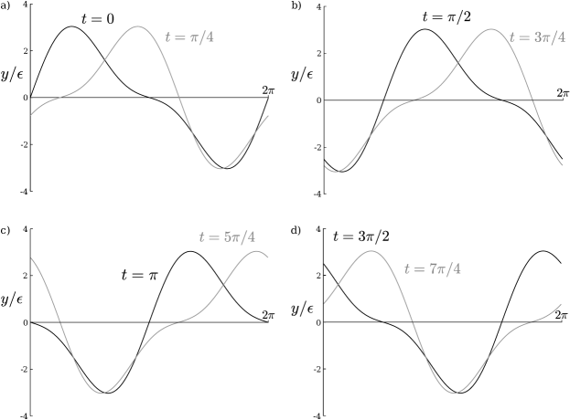
Figure 2: Illustration of a waveform producing faster swimming in a non-Newtonian fluid. The waveform is described by Eq. (37) with $\alpha=5/2$ and $n=2$, and corresponds to a swimming speed ratio as shown by the uppermost solid grey line in Fig. 1a. The black lines in each of the four figures show the waveform at dimensionless times $0$, $\pi/2$, $\pi$ and $3\pi/2$, respectively, and the grey lines show the evolution of the wave an eighth of a period later, to show how the wave travels and changes shape during its period.

Further analytical insight can be provided by noting from Fig. 1 that the peak swimming speed ratio occurs when ${\rm De}$ is order one. Dividing the result in Eq. (39) by that in Eq. (38) and taking a first derivative with respect to ${\rm De}$ we can compute the value of the Deborah number at which the velocity ratio is extremized. It occurs for two values of ${\rm De}$ given by

$${\rm De}_{1\ast}=\sqrt{{\frac{n^{2}-\alpha}{n^{2}(\alpha-1)}}}\,\,\text{and}\,\,{\rm De}_{2\ast}=0.$$ (41)

For $\alpha$ above $n^{2}$ the only solution is the maximum value of 1 occurring at ${\rm De}_{2\ast}=0$. When $\alpha$ crosses below $n^{2}$ a maximum is created near ${\rm De}_{1\ast}=0$, and increases as $\alpha$ decreases. When $\alpha=n$ a transition occurs where ${\rm De}_{1\ast}$ changes from a maximum point ($n<\alpha$) to a minimum ($\alpha<n$); its value at that point is ${\rm De}_{1\ast}=1/n$. It remains a minimum until $\alpha$ crosses the value 1, below which the only solution is the maximum of 1 at ${\rm De}_{2\ast}=0$.

A final point of interest in Fig. 1 is the fact, as discussed above, that the ratio between the swimming speeds can become negative. In these cases, the swimmer would then swim in different directions in the Newtonian and non-Newtonian fluids, as was already noted in Ref. Wolgemuth2007 . This occurs when $\alpha<n$, and the speed ratio goes through a minimum before increasing back towards $\beta$ at large Deborah numbers. The reversal of swimming occurs when there is a difference in sign between Eq. (38) and Eq. (39), which corresponds to the amplitude range

$$\sqrt{\frac{n^{2}(1+\beta n^{2}{\rm De}^{2})(1+{\rm De}^{2})}{(1+n^{2}{\rm De}^{2})(1+\beta{\rm De}^{2})}}<\alpha<n.$$ (42)

This result is reminiscent of a recent study on reciprocal (time-reversible) motion in a worm-like micellular solution, which showed that the direction and the speed of the swimmer could be changed when distinct Deborah numbers are reached Gagnon2014 . Finally, we can also find a range of a values for which the swimmer will not only change direction but will also swim with a larger magnitude, which occurs when

$$\sqrt{\frac{n^{2}(1+\beta n^{2}{\rm De}^{2})(1+{\rm De}^{2})}{(1+n^{2}{\rm De}^{2})(1+\beta{\rm De}^{2})}-1}<\alpha<n.$$ (43)

Here the swimming speed ratio becomes negative and less than $-1$.

IV.2 Necessary vs. sufficient condition for enhanced swimming

The sufficient condition for enhancement derived in §III detailed the conditions required for an upwards curving of the swimming speed ratio from zero Deborah number. In order to study if this sufficient condition is also necessary, we search analytically for the conditions leading to $U_{2NN}>U_{2N}$, leading to

$$0<{\rm De}<\sqrt{\frac{n^{4}-\alpha^{2}}{n^{2}(\alpha^{2}-n^{2})}}\equiv{\rm De}_{a}.$$ (44)

This condition requires $n<\alpha<n^{2}$, and defines the range of Deborah number where forward swimming enhancement is achieved, namely $[0,{\rm De}_{a}]$. If we enforce the curvature to be negative then we cannot find a set of viable parameters for which $U_{2NN}>U_{2N}>0$, thus showing that the sufficient condition is also necessary when two modes are considered: in the case of two waves, if forward swimming enhancement is ever to be obtained, it will take place for any Deborah number below a critical value ${\rm De}_{a}$.

IV.3 Swimming efficiency

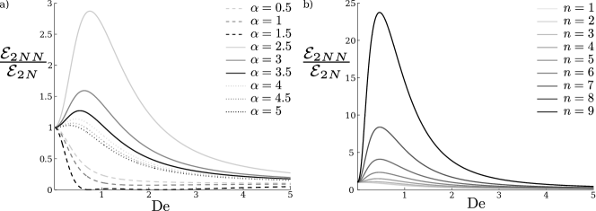
Figure 3: Ratio of the swimming efficiency in a non-Newtonian fluid compared to its Newtonian counterpart as a function of ${\rm De}$: (a) $n=2$ for a range of values of $\alpha$; (b) $\alpha=9.5$ and $1\leq n\leq 9$. The waveform is the one described in Eq. (37).

We now turn to energetic considerations. The rate of viscous dissipation in the fluid as the sheet is swimming is equal to the volume integral of $\boldsymbol{\tau}:\dot{\boldsymbol{\gamma}}$ in the fluid. At leading order we therefore have to integrate $\boldsymbol{\tau}_{1}:\dot{\boldsymbol{\gamma}}_{1}$. With the general waveform in Eq. (1), the dimensional second-order dissipation rate in the non-Newtonian fluid per unit length in the $\mathbf{e}_{z}$ direction is easily found and we obtain $W=\epsilon^{2}W_{2NN}+\dots$ with

$$W_{2NN}=\sum\limits_{n\geq 1}\sum\limits_{m\geq 1} 8\pi\eta\omega^{2}mn^{2}$$

$$\left(\frac{1+n^{2}\beta{\rm De}^{2}}{1+n^{2}{\rm De}^{2}}\right)\left(|\alpha_{n,m}|^{2}-|\alpha_{n,-m}|^{2}\right).$$ (45)

The result in Eq. (IV.3) should then be compared with its Newtonian counterpart.

Let us consider for illustration the waveform in Eq. (37). In that case, the ratio of the work done against the non-Newtonian fluid compared to the Newtonian one is given by

$$\frac{W_{2NN}}{W_{2N}}= \frac{\eta}{\eta_{N}(n^{3}+\alpha^{2})}\times$$

$$\left[\alpha^{2}\left(\frac{1+{\rm De}^{2}\eta_{s}/\eta}{1+{\rm De}^{2}}\right)+n^{3}\left(\frac{1+n^{2}{\rm De}^{2}\eta_{s}/\eta}{1+n^{2}{\rm De}^{2}}\right)\right],$$ (46)

where $\eta_{N}$ is the Newtonian viscosity. In order to contrast the locomotion in the polymeric fluid with that in the solvent alone, we then take $\eta_{N}=\eta_{s}$. Furthermore, as is done traditionally, the swimming efficiency is defined as

$$\mathcal{E}=\frac{\eta U^{2}}{W}\cdot$$ (47)

In order to compare the efficiency of swimming in the different fluids, we compute the ratio

$$\frac{\mathcal{E}_{2NN}}{\mathcal{E}_{2N}}=\frac{\eta U_{2NN}^{2}}{W_{2NN}}\frac{W_{2N}}{\eta_{N}U_{2N}^{2}}\cdot$$ (48)

The ratio of the work and viscosity in the two different fluids, $\eta W_{2N}/\eta_{N}W_{2NN}$, is always greater than $1$ for non-zero Deborah number, meaning that when the swimming speed ratio $U_{2NN}/U_{2N}$ is greater than $1$, the swimming efficiency is automatically always increased.

We plot the ratio of efficiencies against ${\rm De}$ for a range of relative wave amplitude $\alpha$, and wavenumber ratio $n$, in Fig. 3, where $\eta_{s}/\eta=\beta=0.1$. Clearly, an increase in swimming speed is correlated with an increase in efficiency, but increased efficiencies can in fact be obtained without enhanced swimming. Indeed, increased efficiency is obtained as soon as

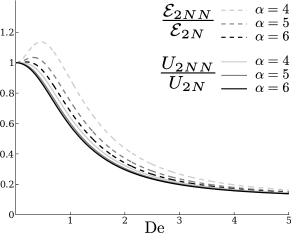
Figure 4: Three example waveforms are shown for which the swimming speed is not enhanced but the efficiency is. The relative amplitude in Eq. (37) lies outside the range $n<\alpha<n^{2}$ ($n=2$).

$$\left(\frac{U_{2NN}}{U_{2N}}\right)^{2}>\frac{\eta_{N}W_{2NN}}{\eta W_{2N}}\cdot$$ (49)

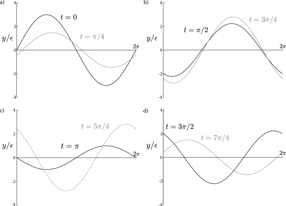
Figure 5: Illustration of a waveform from Eq. (51) with $\alpha=2$ and $n=2$ that produces faster swimming in a non-Newtonian fluid. The black lines in each of the four figures show the waveform at dimensionless times $0$, $\pi/2$, $\pi$ and $3\pi/2$, respectively, and the grey lines show the evolution of the wave an eighth of a period later.

Given that the right-hand side of Eq. (49) is less than one, the condition for enhanced efficiency does not require enhanced swimming. Specifically, using the illustrative sinusoidal waveform of Eq. (37), we obtain an improved efficiency when

$$\frac{\displaystyle(n^{3}+\alpha^{2})}{(\alpha^{2}-n^{2})^{2}}>\displaystyle\frac{\displaystyle\left[\alpha^{2}\left(\frac{1+\beta{\rm De}^{2}}{1+{\rm De}^{2}}\right)+n^{3}\left(\frac{1+\beta n^{2}{\rm De}^{2}}{1+n^{2}{\rm De}^{2}}\right)\right]}{\displaystyle\left[\alpha^{2}\left(\frac{1+\beta{\rm De}^{2}}{1+{\rm De}^{2}}\right)-n^{2}\left(\frac{1+\beta n^{2}{\rm De}^{2}}{1+n^{2}{\rm De}^{2}}\right)\right]^{2}},$$ (50)

for which $n<\alpha<n^{2}$ is not a necessary condition. This result is illustrated in Fig. 4 in the case $n=2$. When $\alpha>n^{2}$, the waveform travels in the same direction in both fluids and the swimmer is always faster in a Newtonian fluid although it is more efficient in the non-Newtonian one for a range of Deborah numbers.

IV.4 Two waves with identical wavelengths

Instead of two waves with identical wave speeds, enhanced swimming can also be obtained in a combination of waves with identical wavelengths. Since the waves need to have different frequencies, then they necessarily have different wave speeds. As an example we consider here the waveform

$$y=\epsilon[\alpha\sin(x-t)+\sin(x+nt)].$$ (51)

This gives

$$U_{2NN}=\frac{\alpha^{2}}{2}\left(\frac{1+\beta{\rm De}^{2}}{1+{\rm De}^{2}}\right)-\frac{n}{2}\left(\frac{1+n^{2}{\rm De}^{2}}{1+n^{2}{\rm De}^{2}}\right),$$ (52)

and

$$U_{2N}=\frac{1}{2}(\alpha^{2}-n).$$ (53)

Similarly as above, the second derivate of $U_{2NN}/U_{2N}$ at ${\rm De}=0$ is given by

$$\frac{\partial^{2}}{\partial{\rm De}^{2}}\left(\frac{U_{2NN}}{U_{2N}}\right)\bigg{|}_{{\rm De}=0}=\left(\frac{\alpha^{2}-n^{3}}{\alpha^{2}-n}\right)(\beta-1),$$ (54)

and faster swimming occurs when

$$n^{1/2}<\alpha<n^{3/2},$$ (55)

which is confirmed by numerical computations (not shown). A waveform leading to enhanced swimming in this case is illustrated in Fig. 5, in the case $\alpha=2$ and $n=2$. This corresponds to a maximum speed enhancement of $U_{2NN}/U_{2N}\approx 1.1$ at Deborah number ${\rm De}\approx 0.4$. To obtain the optimal Deborah number, we extremise the ratio of swimming speeds to find the peaks occurring at

$${\rm De}_{1\ast}=\sqrt{\frac{n^{2}-\alpha\sqrt{n}}{n^{2}(\alpha\sqrt{n}-1)}}\,\,\text{and}\,\,{\rm De}_{2\ast}=0,$$ (56)

with a behavior qualitatively similar to that of the last section.

V Superposition of three travelling waves: continuous vs. discrete enhancement

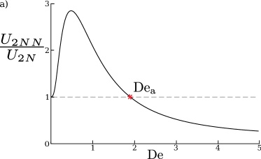
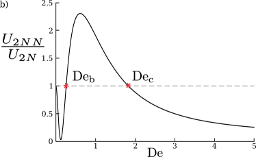
Figure 6: Two different types of enhancement are shown for two different three-mode waves with $n_{1}=1$, $n_{2}=4$ and $n_{3}=8$: (a) continuous enhancement from zero Deborah number in the range $[0,{\rm De}_{a}]$ with ${\rm De}_{a}\approx 1.9$ ($a_{n_{1}}=1$, $a_{n_{2}}=-1$, $a_{n_{3}}=0.3$); (b) enhancement in a discrete, finite, range of Deborah numbers, $[{\rm De}_{b},{\rm De}_{c}]$, where ${\rm De}_{b}\approx 0.3$ and ${\rm De}_{c}\approx 1.8$ ($a_{n_{1}}=1$, $a_{n_{2}}=-2$, $a_{n_{3}}=1.2$).

In the previous sections, where the superposition of two waves was considered, we saw that when enhancement is present, it is continuous from ${\rm De}=0$ to an order one Deborah number ${\rm De}_{a}$, where the value ${\rm De}_{a}\neq 0$ is the only non-zero solution of $U_{2NN}/U_{2N}=1$. We now demonstrate that if the swimmer is able to use a third travelling wave, it is possible for swimming enhancement to occur only when a finite amount of viscoelasticity is present, i.e. for values of the Deborah number in the range $[{\rm De}_{b},{\rm De}_{c}]$, where ${\rm De}_{b}$ and ${\rm De}_{c}$ are both non-zero.

We consider, for illustration purposes, a waveform with three modes $1<n_{2}<n_{3}$. The corresponding square amplitudes $a_{1}$, $a_{n_{2}}$ and $a_{n_{3}}$ are non-dimensionalised by $a_{1}$ so that we take $a_{1}=1$. Using the same notation as above, the Newtonian swimming speed is then given by

$$U_{2N}=1+a_{n_{2}}+a_{n_{3}}.$$ (57)

The difference between the non-Newtonian and Newtonian swimming speeds is then found to be

$$U_{2NN}-U_{2N}= {\rm De}^{2}(\beta-1)\Bigg{[}\left(\frac{1}{1+{\rm De}^{2}}\right)$$

$$+\left(\frac{n_{2}^{2}a_{n_{2}}}{1+n_{2}^{2}{\rm De}^{2}}\right)+\left(\frac{n_{3}^{2}a_{n_{3}}}{1+n_{3}^{2}{\rm De}^{2}}\right)\Bigg{]}.$$ (58)

Focusing on cases where $U_{2N}>0$, enhanced forward swimming is found when Eq. (V) is positive. As shown in Fig. 6 numerically for $n_{2}=4$ and $n_{3}=8$, there are two types of enhancements possible: either on a range $[0,{\rm De}_{a}]$ where the velocity ratio curves upward at the origin (continuous enhancement, Fig. 6a, as in § IV) or on a range $[{\rm De}_{b},{\rm De}_{c}]$ for which the curvature at ${\rm De}=0$ is initially negative before curving upward as the viscoelasticity increases (discrete enhancement, Fig. 6b).

Figure 7: Regions in the parameters space {$a_{n_{2}},a_{n_{3}}$} where enhanced swimming occurs. The black section represents where the curvature is positive (i.e. upwards curving) so that from infinitesimally small Deborah number we get an increase in the swimming speed. In contrast, the grey scale section shows regions where enhanced swimming is obtained despite negative curvature at the origin. The grey scale color scheme quantifies the value of non-zero Deborah numbers at which the increase in swimming speed first occurs, ${\rm De}_{b}$, from low Deborah number in dark, to high Deborah number ($\approx 0.8$) in light grey. Results are shown for $n_{2}=4$ and $n_{3}=8$.

In order to distinguish between them analytically, we observe that when the curvature is negative, we can either have no enhancement or enhancement at a finite Deborah number. Hence, we need to search for cases where Eq. (V) is positive, given that the curvature at the origin is negative. The curvature of the general wave was obtained in Eq. (35), hence for negative curvature in our three-mode waveform we require

$$\kappa=2(\beta-1)(1+n_{2}^{2}a_{n_{2}}+n_{3}^{2}a_{n_{3}})<0.$$ (59)

The result in Eq. (V) can then be written in terms of $U_{2N}$ and $\kappa$ as

$$n_{2}^{2}n_{3}^{2}{\rm De}^{4}(\beta-1) \left(\frac{n_{2}^{2}+n_{3}^{2}-1}{n_{2}^{2}n_{3}^{2}}+a_{n_{2}}+a_{n_{3}}\right)>$$

$$\left[{\rm De}^{2}\kappa(\tfrac{1}{2}+{\rm De}^{2})+n_{2}^{2}n_{3}^{2}{\rm De}^{4}(\beta-1)U_{2N}\right].$$ (60)

As $\beta-1<0$, and assuming that $U_{2N}>0$ and $\kappa<0$, the minimum requirement for non-continuous enhancement is

$$\frac{n_{2}^{2}+n_{3}^{2}-1}{n_{2}^{2}n_{3}^{2}}+a_{n_{2}}+a_{n_{3}}<0.$$ (61)

The three conditions given by Eqs. (57) ($U_{2N}>0$), (59), and (61) can be satisfied simultaneously only when $a_{n_{2}}<0$ and $a_{n_{3}}>0$, i.e. the first and third modes must have a different sign to the second mode. We then search numerically over the domain {$a_{n_{2}}<0$, $a_{n_{3}}>0$} and ${\rm De}$ to obtain the regions where Eq. (V) is positive provided $U_{2N}>0$ and $\kappa<0$, in the example case $n_{2}=4$ and $n_{3}=8$. The values of $a_{n_{2}}$ and $a_{n_{3}}$ fitting these conditions are shown in Fig. 7 (grey scale domain) while the region showing continuous enhancement is shown in black. The grey scale colouring scheme used in Fig 7 displays the value of the lower bound in the interval, ${\rm De}_{b}$, from low (dark grey) to high (light grey) values. For three waves, in contrast to the case of two waves, situations exist therefore where a finite amount of viscoelasticity is required to get enhanced propulsion, ${\rm De}>{\rm De}_{b}>0$ (analysis for four and five mode waves show similar results and are not shown here).

VI Discussion and conclusion

Motivated by the non-Newtonian environment in which many swimmers propel themselves in vivo, in this paper, we have calculated the speed of Taylor’s swimming sheet in a Newtonian and an Oldroyd-B (non-Newtonian) fluid, in the small-amplitude limit. In contrast to previous analytical studies, we found that small-amplitude travelling waves can produce faster swimming in a non-Newtonian fluid compared to a Newtonian fluid when there are waves travelling in opposite directions in different frequency modes and with different amplitudes. Physically, in a non-Newtonian fluid the waves in higher frequency modes are damped more than those in lower frequency modes, increasing the overall speed of the wave under conditions placed upon the difference in frequency and amplitude of the summed waveforms. The efficiency of the wave can also be increased, and the direction of swimming can sometimes be reversed. By studying in detail the superposition of two or three travelling waves, we also showed that the range of Deborah number in which the enhancement of the swimming speed takes place can either include the origin, in which case any small amount of viscoelasticity will lead to faster swimming, or it may be a finite interval which does not include the origin, meaning that faster locomotion requires a finite amount of viscoelasticity.

The results in this paper are reminiscent of recent experimental and theoretical work on the role of inertia in locomotion, where two important questions have been addressed: (1) for a non-swimmer at zero Reynolds numbers, how much inertia is needed to make it swim? and (2) how does the locomotion speed of a Stokesian swimmer vary with inertia? The answer to question (1) depends crucially on the geometry and actuation of the swimmer and both discrete Alben2004 ; Vandenberghe2004 and continuous Lauga2007P transition to swimming were obtained. In response to question (2), model organisms called squirmers were shown to vary their speed monotonically from zero Reynolds number Wang2012 ; khair2014expansions . Similarly, in our results, we showed that a careful design of the swimming kinematics could lead to either a decrease or an increase, which could be continuous or discrete, of the locomotion speed. We expect that these results will remain valid for more realistic models of swimming organisms, in particular those including features such as large-amplitude, finite-size, and three-dimensional effects.

In three-dimensions, the same frequency-dependent damping term as the one in Eq. (30) is present for infinite cylindrical swimmers FuWolgemuthPowers2009 , hence similar results are expected to hold. With regards to finite sized swimmers, backward propagating waves are expected to occur due to the finite nature of real flagella. Previous computational studies have shown that the addition of viscoelasticity decreases the backwards motion of a finite swimmer Shelley2010 due to the presence of a viscoelastic network behind the swimmer. The opposite has been observed experimentally for nematodes where hyperbolic stresses created along the swimmer hinder propulsion Arratia2011 . It is yet unclear how our theoretical results would extend to a finite swimmer, though we may expect that the mechanism provided in this paper would provide an additional contribution to the swimming speed. In the case of multiple swimmers, it would be interesting to investigate how waves with both high and low frequency modes affect one another and potentially synchronise. From Ref Elfring2010 we expect the synchronisation rate to increase with the frequency of the waves however the generalisation to multiple modes in viscoelastic fluids has yet to be done. A recent study address a related issue in the Newtonian case Brumley2014 .

The waveforms produced here offer insight into how swimming speeds can be increased in fluids with viscoelastic properties often found in nature RheoBook . Can these shape kinematics occur in biology? For flagellar swimming this requires understanding of how the stochastic actuation of molecular motors create waveforms. Dynein, the motor protein causing flagella bending, has been proposed to have two distinct modes to create oscillatory bending - these can be described as active and passive, or forward and reverse active modes Brokaw2009 , leading to travelling waves that can propagate up or down the flagellum. Due to the finite nature of flagella the wave is reflected back off the tail end or basal body, thus creating passive backwards waves Machin1958 . Experiments on Drosophila spermatozoa show that the cells use actively created forwards and backwards flagellar waves to avoid obstacles Yang2011 . Furthermore by solving elastohydrodynamic force balance equations on infinite flagella analytic studies have shown two different modes of waves travel along the flagella with the same frequency, but different amplitudes and directions Wiggins1998 . Hence a flagellum naturally creates forward and backward travelling waves with different amplitudes. The enhancement described in this paper requires however waves with different frequencies travelling in the backwards direction for enhancement to occur. The addition of higher frequency modes ($n=2$ and $n=3$), found in small amounts in beating spermatozoa ReidelKruse2007 , would not however lead to an increase in swimming speed as $a_{n}>0$ for all values of $n$ found experimentally. Changes in flagella beating frequency can occur by altering the environment in which the swimmer propagates, for example hyperactivation when mammalian spermatozoa reach the ovum, leading to a reduction in the beat frequency and increase in the beat amplitude Suarez1991 ; a variation in ATP or salt concentrations also change frequencies Brokaw2009 . Recent work on the unsteady modes of flagellar motion show that most modes have a frequency smaller than the fundamental frequency, and hence would correspond to a reduced swimming speed Bayly2015 . The addition of noise to the molecular motor oscillations, either through variations in concentrations in the bulk or variations between motors, could lead to increased swimming provided the coherent noise is large enough for the flagellum to access a higher frequency mode, however this is larger than the noise measured Ma2014 . Backwards travelling wave results have been described for muscle-actuated planar motion occurring for example in the nematode Caenorhabditis elegans Sznitman2010 as well as other flagellar systems such as the green alga Chlamydomonas reinhardtii Guasto2010 .

While our study offers only an idealised view, and although as of yet there are no experimental studies from biology for which the model here would predict faster swimming, our work address the most general periodic waving deformation and points to the use of multiple waves travelling in different directions as a mechanism allowing control of swimming magnitude and direction in complex environments.

References

- [1] E. M. Purcell. The efficiency of propulsion by rotating flagellum. Proc. Natl. Acad. Sci. USA, 94:11307–11311, 1997.
- [2] C. Brennen and H. Winet. Fluid mechanics of propulsion by cilia and flagella. Ann. Rev. Fluid. Mech., 9:339–398, 1977.
- [3] E. Lauga and T. R. Powers. The hydrodynamics of swimming microorganisms. Rep. Prog. Phys., 72:096601–096637, 2009.
- [4] M. A. Sleigh, J. R. Blake, and N. Liron. The propulsion of mucus by cilia. Am. Rev. Respir. Dis., 137:726–741, 1988.
- [5] H. R. Wallace. The dynamics of nemotode movement. Annu. Rev. Phytopathol, 6:91–114, 1967.
- [6] C. Josenhans and S. Suerbaum. The role of motility as a virulence factor in bacteria. International Journal of Medical Microbiology, 291:605–614, 2002.
- [7] S. S. Suarez and A. A. Pacey. Sperm transport in the female reproductive tract. Human. Reprod. Update, 12:23–37, 2006.
- [8] D. A. Gagnon, X. N. Shen, and P. E. Arratia. Undulatory swimming in fluids with polymer networks. Europhys. Lett., 104:14004, 2013.
- [9] X. Shen and P. E. Arratia. Undulatory swimming in viscoelastic fluids. Phys. Rev. Lett., 106:208101, May 2011.
- [10] G. I. Taylor. Analysis of the swimming of microscopic organisms. Proc. R. Soc. London Ser. A, 209:447–461, 1951.
- [11] M. Dasgupta, B. Liu, H. C. Fu, M. Berhanu, K. S. Breuer, T. R. Powers, and A. Kudrolli. Speed of a swimming sheet in Newtonian and viscoelastic fluids. Phys. Rev. E, 87:013015, 2013.
- [12] J. Espinosa-Garcia, E. Lauga, and R. Zenit. Fluid elasticity increases the locomotion of flexible swimmers. Phys. Fluids, March 2013.
- [13] E. Lauga. Propulsion in a viscoelastic fluid. Phys. Fluids, 2007.
- [14] T. D. Montenegro-Johnson, D. J. Smith, and D. Loghin. Physics of rheologically-enhanced propulsion: different strokes in generalized Stokes. Phys. Fluids, 25:081903, 2013.
- [15] H. C. Fu, T. R. Powers, and C. W. Wolgemuth. Theory of swimming filaments in viscoelastic media. Phys. Rev. Lett., 99:258101, 2007.
- [16] L. Zhu, M. Do-Quang, E. Lauga, and L. Brandt. Locomotion by tangential deformation in a polymeric fluid. Phys. Rev. E, 83:011901, 2011.
- [17] L. Zhu, E. Lauga, and L. Brandt. Self-propulsion in viscoelastic fluids: pushers vs. pullers. Phys. Fluids, 24:051902, 2012.
- [18] M. P. Curtis and E. A. Gaffney. Three-sphere swimmer in a nonlinear viscoelastic medium. Phys. Rev. E, 87:043006, 2013.
- [19] E. M. Purcell. Life at Low Reynolds Number. Am. J. Phys., 45:3–11, 1977.
- [20] T. Normand and E. Lauga. Flapping motion and force generation in a viscoelastic fluid. Phys. Rev E, 78:061907, November 2008.
- [21] O. S. Pak, L. Zhu, L. Brandt, and E. Lauga. Micropropulsion and microrheology in complex fluids via symmetry breaking. Phys. Fluids, 24:103102, 2012.
- [22] E. Lauga. Life at high Deborah number. Europhys. Lett., 86:64001, 2009.
- [23] E. Lauga. Life around the scallop theorem. Soft Matter, 7:3060–3065, 2011.
- [24] B. Liu, T. R. Powers, and K. S. Breuer. Force-free swimming of a model helical flagellum in viscoelastic fluids. Proc. Natl. Acad. Sci. USA, 108:19516–19520, 2011.
- [25] J. C. Chrispell, L. J. Fauci, and M. Shelley. An actuated elastic sheet interacting with passive and active structures in a viscoelastic fluid. Phys. Fluids, 25:013103, 2013.
- [26] J. Teran, L. Fauci, and M. Shelley. Viscoelastic fluid response can increase the speed and efficiency of a free swimmer. Phys. Rev. Lett., 104:038101, 2010.
- [27] S. E. Spagnolie, B. Liu, and T. R. Powers. Locomotion of helical bodies in viscoelastic fluids: Enhanced swimming at large helical amplitudes. Phys. Rev. Lett., 111:068101, 2013.
- [28] B. Thomases and R. D. Guy. Mechanisms of elastic enhancement and hindrance for finite-length undulatory swimmers in viscoelastic fluids. Phys. Rev. Lett., 113:098102, 2014.
- [29] H. C. Fu, V. B. Shenoy, and T. R. Powers. Low-Reynolds number swimming in gels. Europhys. Lett., 91:24002, 2010.
- [30] A. M. Leshansky. Enhanced low-Reynolds-number propulsion in heterogeneous viscous environments. Phys. Rev. E, 80:051911, 2009.
- [31] E. E. Riley and E. Lauga. Enhanced active swimming in viscoelastic fluids. Europhys. Lett., 108:34003, 2014.
- [32] J. R. Vélez-Cordero and E. Lauga. Waving transport and propulsion in a generalized Newtonian fluid. J. Non-Newt. Fluid Mech., 199:37–50, 2013.
- [33] G. J. Elfring, O. S. Pak, and E. Lauga. Two-dimensional flagellar synchronization in viscoelastic fluids. J. Fluid Mech., 646:505–515, 2010.
- [34] G. R. Fulford, D. F. Katz, and R. L. Powell. Swimming of spermatozoa in a linear viscoelastic fluid. Biorheology, 35:295–309, 1998.
- [35] H. C. Fu, C. W. Wolgemuth, and T. R. Powers. Swimming speeds of filaments in nonlinearly viscoelastic fluids. Phys. Fluids, 21:033102, 2009.
- [36] J. G. Oldroyd. On the formulation of rheological equations of state. Proc. R. Soc. London Ser. A, 200:523, 1950.
- [37] N. Phan-Thien. Understanding Viscoelasticity: An Introduction to Rheology. Graduate Texts in Physics. Springer, 2012.
- [38] D. A. Gagnon, N. C. Keim, X. Shen, and P. E. Arratia. Fluid-induced propulsion of rigid particles in wormlike micellar solutions. Phys. Fluids, 26:103101, 2014.
- [39] S. Alben and M. Shelley. Coherent locomotion as an attracting state for a free flapping body. Proc. Natl. Acad. Sci. USA, 102:11163–11166, 2004.
- [40] N. Vandenberghe, J. Zhang, and S. Childress. Symmetry breaking leads to forward flapping flight. J. Fluid Mech., 506:147–155, 2004.
- [41] E. Lauga. Continuous breakdown of Purcell’s scallop theorem with inertia. Phys. Fluids, 19:061703, 2007.
- [42] S. Wang and A. Ardekani. Inertial squirmer. Phys. Fluids, 24:101902, 2012.
- [43] A. S. Khair and N. G. Chisholm. Expansions at small Reynolds numbers for the locomotion of a spherical squirmer. Phys. Fluids, 26:011902, 2014.
- [44] D. R. Brumley, K. Y. Wan, M. Polin, and R. E. Goldstein. Flagellar synchronization through direct hydrodynamic interactions. eLife, 3:e02750, 2014.
- [45] A. Borzacchiello, L. Ambrosio, P. Netti, and L. Nicolais. Rheology of Biological Fluids and Their Substitues. Marcel Dekker, Inc, 2004.
- [46] C. J. Brokaw. Thinking about flagella oscillation. Cell Motil. Cytoskel., 66:425–436, 2009.
- [47] K. E. Machin. Wave propagation along flagella. J. Exp. Biol., 35:796–806, 1958.
- [48] Y. Yang and X. Lu. Drosophila Sperm Motility in the Reproductive Tract. Biol. Reprod., 84:1005–1015, 2011.
- [49] C. H. Wiggins and R. E. Goldstein. Flexive and propulsive dynamics of elastica at Low Reynolds number. Phys. Rev. Lett., 80, 1998.
- [50] I. H. Reidel-Kruse, A. Hilfinger, J. Howard, and F. Jülicher. How molecular motors shape the flagellar beat. HFSP J., 1:192–208, 2007.
- [51] S. S. Suarez, D. F. Katz, D. H. Owen, J. B. Andrew, and R. L. Powell. Evidence for the function of hyperactivated motility in sperm. Biol. Reprod., 44:375–381, 1991.
- [52] P. V. Bayly and K. S. Wilson. Analysis of unstable modes distinguishes mathematical models of flagellar motion. J. R. Soc. Interface, 12:0124, 2015.
- [53] R. Ma, G. S. Klindt, I. H. Riedel-Kruse, F. Jülicher, and B. M. Friedrich. Active phase and amplitude fluctuations of flagellar bending. Phys. Rev. Lett., 113:048101, 2014.
- [54] J. Sznitman, P. K. Purohit, P. Krajacic, T. Lamitina, and P. E. Arratia. Material properties of Caenorhabditis elegans swimming at low Reynolds number. Biophys. J., 98:617–626, 2010.
- [55] J. S. Guasto, K. A. Johnson, and J. P. Gollub. Oscillatory flows Induced by microorganisms swimming in two dimensions. Phys. Rev. Lett., 105:168102, 2010.