Distinguishing LSP archetypes
via gluino pair production at LHC13

Abstract

The search for supersymmetry at Run 1 of LHC has resulted in gluino mass limits $m_{\tilde{g}}\gtrsim 1.3$ TeV for the case where $m_{\tilde{q}}\gg m_{\tilde{g}}$ and in models with gaugino mass unification. The increased energy and ultimately luminosity of LHC13 will explore the range $m_{\tilde{g}}\sim 1.3-2$ TeV. We examine how the discovery of SUSY via gluino pair production would unfold via a comparative analysis of three LSP archetype scenarios: 1. mSUGRA/CMSSM model with a bino-like LSP, 2. charged SUSY breaking (CSB) with a wino-like LSP and 3. SUSY with radiatively-driven naturalness (RNS) and a higgsino-like LSP. In all three cases we expect heavy-to-very-heavy squarks as suggested by a decoupling solution to the SUSY flavor and CP problems and by the gravitino problem. For all cases, initial SUSY discovery would likely occur in the multi-$b$-jet + $\not{E}_{T}$ channel. The CSB scenario would be revealed by the presence of highly-ionizing, terminating tracks from quasi-stable charginos. As further data accrue, the RNS scenario with 100-200 GeV higgsino-like LSPs would be revealed by the build-up of a mass edge/bump in the OS/SF dilepton invariant mass which is bounded by the neutralino mass difference. The mSUGRA/CMSSM archetype would contain neither of these features but would be revealed by a buildup of the usual multi-lepton cascade decay signatures.

I Introduction

The LHC8 (LHC with $\sqrt{s}=7-8$ TeV) era has come to a close and the LHC13 era is underway! What have we learned from LHC8? The Standard Model (SM) has been spectacularly confirmed in a vast assortment of measurementshinchliffe . And most importantly, a very SM-like Higgs boson has been revealed with mass $m_{h}=125.09\pm 0.24$ GeV (ATLAS/CMS combined)atlas_h ; cms_h . The next major target for LHC is to root out evidence for supersymmetry (SUSY). Indeed, it has been declared that if LHC13 does not uncover evidence for SUSY early within Run 2, then physics will have entered a state of crisisLykken:2014bca !

What we have learned from LHC8 is that– in generic models such as mSUGRA/CMSSM– no evidence for SUSY translates into mass bounds of

$$m_{\tilde{g}}\gtrsim 1.3\ {\rm TeV} \ \ \ {\rm for}\ m_{\tilde{q}}\gg m_{\tilde{g}}\ \ \ {\rm and}$$ (1)

$$m_{\tilde{g}}\gtrsim 1.8\ {\rm TeV} \ \ \ {\rm for}\ m_{\tilde{q}}\sim m_{\tilde{g}}.$$ (2)

In addition, the rather large value of $m_{h}\simeq 125$ GeV seems to require large radiative corrections to $m_{h}^{2}$ in the MSSMmhiggs . The Higgs mass can be accommodated with TeV-scale top squarks for large trilinear soft breaking parameter $A_{0}$h125 , or by 10-100 TeV top squarks in the minimal mixing caseArbey:2011ab . Naively, these rather high sparticle mass limits seem to conflict with notions of weak scale naturalness which favor sparticles at or around $m_{weak}\simeq 100$ GeV, the value of $m_{W,Z,h}$. This has led to some puzzlement as to the emerging Little Hierarchy: why is $m(sparticle)\gg m_{weak}$? It has also led to more detailed examination of what is meant by electroweak naturalness.

The point of contact between SUSY Lagrangian mass parameters (soft terms and superpotential $\mu$ term) and hard data occurs in the scalar (Higgs) potential: in the MSSM, it is given by

$$V_{Higgs}=V_{tree}+\Delta V,$$ (3)

where the tree level portion is given by

$$V_{tree} = (m_{H_{u}}^{2}+\mu^{2})|h_{u}^{0}|^{2}+(m_{H_{d}}^{2}+\mu^{2})|h_{d}^{0}|^{2}$$ (4)

$$-B\mu(h_{u}^{0}h_{d}^{0}+h.c.)+{1\over 8}(g^{2}+g^{\prime 2})(|h_{u}^{0}|^{2}-|h_{d}^{0}|^{2})^{2}$$

and the radiative corrections (in the effective potential approximation) by

$$\Delta V=\sum_{i}\frac{(-1)^{2s_{i}}}{64\pi^{2}}Tr\left(({\cal M}_{i}{\cal M}_{i}^{\dagger})^{2}\left[\log{{\cal M}_{i}{\cal M}_{i}^{\dagger}\over Q^{2}}-{3\over 2}\right]\right),$$ (5)

where the sum over $i$ runs over all fields that couple to Higgs fields, ${\cal M}_{i}^{2}$ is the Higgs field dependent mass squared matrix (defined as the second derivative of the tree level Lagrangian) of each of these fields, and the trace is over the internal as well as any spin indices. Minimization of the scalar potential in the $h_{u}^{0}$ and $h_{d}^{0}$ directions allows one to compute the gauge boson masses in terms of the Higgs field vacuum expectation values $v_{u}$ and $v_{d}$, and leads to the well-known condition that

$$\frac{m_{Z}^{2}}{2}=\frac{(m_{H_{d}}^{2}+\Sigma_{d}^{d})-(m_{H_{u}}^{2}+\Sigma_{u}^{u})\tan^{2}\beta}{(\tan^{2}\beta-1)}-\mu^{2},$$ (6)

where the $\Sigma_{u}^{u}$ and $\Sigma_{d}^{d}$ terms arise from derivatives of $\Delta V$ evaluated at the potential minimum and $\tan\beta\equiv\frac{v_{u}}{v_{d}}$. This minimization condition relates the $Z$-boson mass scale to the soft SUSY breaking terms and the superpotential higgsino mass $\mu$. In most computations of the SUSY mass spectrum, the weak scale soft terms are determined by renormalization group running from a constrained set of parameters set at some high scale $\Lambda$. In gravity-mediationsugra , $\Lambda$ is usually taken to be $m_{GUT}\simeq 2\times 10^{16}$ GeVsugreview . Then the weak scale value of $\mu$ is dialed (fine-tuned) so that the measured value of $m_{Z}$ is obtained. An evaluation of the extent of this fine-tuning is provided by the electroweak measure $\Delta_{EW}$ which evaluates the largest of the 43 terms on the right-hand-side of Eq. 6. If one term on the RHS is $\gg m_{Z}^{2}$, then some other unrelated term will have to be large and of opposite-sign to guarantee that $m_{Z}=91.2$ GeV. To avoid such large weak scale tuning, evidently all terms on the right-hand-side of Eq. 6 should be comparable to or less than $m_{Z}^{2}$. This implies the followingltr ; rns .

• The superpotential higgsino mass $\mu\sim 100-200$ GeV, the closer to $m_{Z}$ the better. The lower limit $\mu\gtrsim 100$ GeV comes from null searches for chargino pair production at LEP2.

• The soft term $m_{H_{u}}^{2}$ is radiatively driven to small values $\sim-m_{Z}^{2}$ at the weak scale.

• The radiative corrections $\Sigma_{u}^{u}$ are not too large. The largest of these usually comes from the top-squarks. Each of the terms $\Sigma_{u}^{u}(\tilde{t}_{1,2})$ are minimized by TeV-scale highly mixed top squarks, a condition which also lifts $m_{h}$ up to $\sim 125$ GeVltr ; rns .

Some alternative fine-tuning measures also have been advocated in the literature.

1. The usual application of the Higgs mass large-log measure $\Delta_{HS}=\delta m_{H_{u}}^{2}/(m_{h}^{2}/2)$ where $\delta m_{H_{u}}^{2}\sim\frac{f_{t}^{2}}{8\pi^{2}}\left(m_{Q_{3}}^{2}+m_{U_{3}}^{2}+A_{t}^{2}\right)\ln\left(\Lambda/m_{SUSY}\right)$ has been challengedcomp3 ; seige in that it ignores the dependent term $m_{H_{u}}^{2}$ which occurs in the RGE. But the larger $m_{H_{u}}^{2}(\Lambda)$ becomes, the greater is the cancelling correction to $\delta m_{H_{u}}^{2}$arno . By appropriately combining dependent terms, $\Delta_{HS}$ reduces to the same general consequences as $\Delta_{EW}$.

2. Alternatively, the Ellis et al./Barbieri-Giudice measureeenz ; bg is defined as $\Delta_{BG}\equiv\max_{i}|\partial\ln(m_{Z}^{2})/\partial p_{i}|$ where the $p_{i}$ constitute fundamental high scale parameters of the theory. To evaluate $\Delta_{BG}$, $m_{Z}^{2}$ must be evaluated in terms of fundamental high scale parameters usually taken to be the GUT scale soft breaking terms. The usual application of this measure has been challengedcomp3 ; seige in that in supergravity theories, the soft terms are not independent, but are evaluated as multiples of the fundamental gravitino mass $m_{3/2}$. Evaluating $\Delta_{BG}$ in terms of the independent parameters $\mu$ and $m_{3/2}$, low $\Delta_{BG}$ also leads to the same general consequences as $\Delta_{EW}$.

Using $\Delta_{EW}$, then indeed most constrained high scale SUSY models are found to be highly tuned in the EW sectorseige . An exception occurs for a pocket of parameter space of the two-extra parameter non-universal Higgs modelsnuhm2 where $\mu\sim 100-200$ GeV and where $m_{H_{u}}^{2}$ is driven to small negative values comparable to $-m_{Z}^{2}$ while allowing for highly mixed TeV-scale top squarks which provide $m_{h}\simeq 125$ GeV. This pocket of parameter space we call SUSY with radiatively-driven naturalness, or RNS for short. By requiring EW naturalness, then upper bounds can be computed for all sparticle massesrns . In radiative natural SUSY with $\Delta_{EW}<10\ (30)$ then it is found thatrns :

• $m_{\tilde{g}}\lesssim 2.5\ (5)$ TeV,

• $m_{\tilde{t}_{1}}\lesssim 2\ (3)$ TeV,

• $m_{\widetilde{W}_{1},\widetilde{Z}_{1,2}}\lesssim 200\ (300)$ GeV.

The first of these values can be compared to the ultimate reach of LHC14 with 1000 fb^-1 where a $5\sigma$ discovery can be established for $m_{\tilde{g}}\lesssim 2$ TeVbblt ; rns@lhc . Thus, while EW naturalness certainly allows for gluinos and squarks to lie well beyond the ultimate reach of LHC13, it is also true that the most natural values of gluino and squark masses are those within the exploratory range of LHC13: the lighter the better. This motivates an examination of how a SUSY discovery via gluino pair production is likely to unfold at LHC13 when the gluino mass lies just beyond present bounds.

In this paper we assume a gluino mass of $m_{\tilde{g}}=1400$ GeV, i.e. just beyond present bounds. We then investigate how a SUSY discovery would unfold under three lightest SUSY particle (LSP) archetype scenarios:

• the mSUGRA/CMSSM model with a bino-like LSP,

• a charged SUSY breaking (CSB) scenario with a wino-like LSP and

• SUSY with radiatively-driven naturalness and a higgsino-like LSP.

Our goal is to look for commonalities and differences between these three archetype scenarios that would allow a rapid determination of the nature of the LSP if a gluino pair production signal emerges at LHC13.

Towards this end, in Sec. II, we present three archetype benchmark models (BM) labelled as mSUGRA, CSB and RNS. While each BM model contains a gluino with mass 1400 GeV, their implications for collider searches will be very different. In Sec. III, we discuss how SUSY discovery would unfold in each BM model while in Sec. IV we discuss how each archetype could ultimately be distinguished as more integrated luminosity accrues. Briefly, in all cases the most likely initial discovery channel could occur in the multi-$b$-jet + $\not{E}_{T}$ channel with $\sim 3-8$ fb^-1 of integrated luminosity. For the CSB benchmark, the model would be distinguished by the presence of one or more cm-length highly ionizing tracks (HITs) from quasi-stable charginos which are produced within the gluino cascade decays. For the RNS scenario, as 100-1000 fb^-1 of integrated luminosity accumulates, then a distinctive opposite-sign/same flavor (OS/SF) dilepton invariant mass edge should develop in multi-$b$-jet + $\not{E}_{T}$ events which contain such a dilepton pair. The mass edge occurs at the kinematic limit $m(\ell^{+}\ell^{-})<m_{\widetilde{Z}_{2}}-m_{\widetilde{Z}_{1}}\sim 10-30$ GeV in RNS models. For the mSUGRA benchmark, neither of the above distinctive features should develop, but instead the usual multi-lepton plus multijet + $\not{E}_{T}$ cascade decay topologies should build up as greater integrated luminosity accrues. Our summary and conclusions are given in Sec. V.

II Benchmark Models

In this section, we present three benchmark models representing each of three LSP archetype scenarios. Each scenario contains a light Higgs scalar $m_{h}\simeq 125$ GeV and a gluino of mass $m_{\tilde{g}}=1.4$ TeV, just beyond the bounds from LHC8. All spectra were generated using the Isajet/Isasugra 7.84 programisajet .

II.1 mSUGRA/CMSSM

In the minimal supergravity model (mSUGRA or CMSSM)sugra , it is assumed that supergravity is broken in a hidden sector leading to a massive gravitino characterized by mass $m_{3/2}$, with $m_{3/2}\sim 1$ TeV in accord with phenomenological requirements. In the limit as $M_{P}\rightarrow\infty$ but keeping $m_{3/2}$ fixed, then one is lead to the global SUSY Lagrangian of the MSSM augmented by soft SUSY breaking terms each of order $m_{3/2}$. A simplifying assumption (with minimal motivation) is that all soft scalar masses are unified to $m_{0}$ at the GUT scale. In addition, all gaugino masses are unified to $m_{1/2}$, all trilinears are unified to $A_{0}$ and there is a bilinear term $B$. Renormalization group running connects the GUT scale parameters to the weak scale ones. At the weak scale, the scalar potential is minimized and the superpotential $\mu$ parameter is dialed (fine-tuned) so as to generate the measured value of $m_{Z}=91.2$ GeV.

Spectra from this popular model Ross:1992tz ; Arnowitt:1992aq ; Barger:1992ac ; Barger:1993gh can be generated with many computer codes. In Table 1, we show a mSUGRA benchmark model with $m_{0}=5$ TeV, $m_{1/2}=517$ GeV, $A_{0}=-8$ TeV and the ratio of Higgs vevs $\tan\beta=10$. These parameters lead to a spectra with a gluino mass $m_{\tilde{g}}=1.4$ TeV, i.e. just beyond the reach of LHC8. The light Higgs mass $m_{h}=123.6$ GeV, in accord with its measured value if one allows for the $\pm 2$ GeV uncertainty in our calculation of $m_{h}$. The $\widetilde{Z}_{1}$ is a bino-like LSP. The superpotential $\mu$ parameter turns out to be $\mu=2861$ GeV leading to $\Delta_{EW}=1968$ so that this benchmark is highly fine-tuned in the EW sector. The calculated thermal neutralino abundance $\Omega_{\widetilde{Z}_{1}}^{TP}h^{2}=317$, far beyond the measured value. Thus, some sort of 1. late entropy dilution, 2. decay of $\widetilde{Z}_{1}$ to an even lighter LSP such as an axino or 3. $R$-parity violating decays of $\widetilde{Z}_{1}$ would need to be invoked to bring the model into accord with the measured dark matter density. A schematic illustration of the lighter spectral states of the mSUGRA benchmark is shown in Fig. 1.

	mSUGRA	CSB	RNS
$m_{0}$	5,000	50,570	5,000
$M_{1}$	517.0	927.3	517.8
$M_{2}$	517.0	140.5	517.8
$M_{3}$	517.0	-421.5	517.8
$A_{0}$	-8,000	140.5	-8,000
$\tan\beta$	10	10	10
$\mu$	2,861	2,000	150
$m_{A}$	5,666	2,000	2,000
$m_{h}$	123.6	126.4	124.1
$m_{\tilde{g}}$	1,400	1,399	1,399
$m_{\tilde{u}_{L}}$	5,065	50,205	5,038
$m_{\tilde{t}_{1}}$	1,929	34,327	1,332
$m_{\tilde{W}_{2}}$	2.872.0	2,064.8	464.3
$m_{\tilde{W}_{1}}$	460.8	143.6	150.7
$m_{\tilde{Z}_{4}}$	2,866.3	2,062.8	473.6
$m_{\tilde{Z}_{3}}$	2,865.1	2,062.2	243.3
$m_{\tilde{Z}_{2}}$	459.8	438.8	159.5
$m_{\tilde{Z}_{1}}$	234.3	143.4	132.1
Bino frac.	0.9999	0.0022	0.2915
Wino frac.	0.0010	0.9993	0.1747
Higgsino frac.	0.0151	0.0365	0.9405
$\Omega_{\widetilde{Z}_{1}}^{TP}h^{2}$	317	0.0013	0.01
$\Delta_{EW}$	1968	5228	10.4

Table 1: Input parameters and masses (in GeV) for three benchmark points computed with ISAJET 7.84 isajet . Also displayed are the bino, wino and Higgsino fractions.

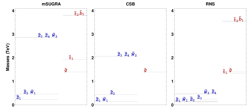
Figure 1: Spectra of benchmark models: mSUGRA (left), CSB (middle), RNS (right). We display the bottom part of the spectra up to 4 TeV where the electroweak -ino’s are shown in blue while the gluinos, stops and sbottoms are shown in red. The sparticles within the same column are ordered in increasing mass from left to right. In the CSB model, the stop and sbottom masses are $\sim 35$ TeV: see Table 1.

II.2 Charged SUSY breaking

In models labeled as minimal anomaly-mediation (mAMSB)amsb , it is assumed that SUSY is broken in a secluded sector so that the dominant contributions to soft terms come not from tree-level supergravity but from the superconformal anomaly. Such models leads characteristically to spectra including wino-like gauginos as the lightest SUSY particlesamsb_pheno . Further, one obtains spectra with well-known tachyonic sleptons. In the original constructamsb , it was suggested to augment soft scalar masses with a common $m_{0}^{2}$ term to cure the tachyon problem.

The original mAMSB models seem disfavored in that they have problems generating $m_{h}\simeq 125$ GeV due to a rather small weak scale $A_{t}$ soft termArbey:2011ab ; dm125 . An alternative incarnation goes under the label of PeV SUSYwells , split SUSYsplit , pure gravity mediationyanagida and spread SUSYhall . In the simple yet elegant construction of Wellswells , it is argued that the PeV scale (with $m({\rm scalars})\sim m_{3/2}\sim 1$ PeV$=$1000 TeV) is motivated by considerations of wino dark matter and neutrino mass while providing a decoupling solution dine to the SUSY flavor, CP, proton decay and gravitino/moduli problems. This model invoked “charged SUSY breaking” (CSB) where the hidden sector superfield $S$ is charged under some unspecified symmetry. In such a case, the scalars gain masses via SUGRA

$$\int d^{2}\theta d^{2}\bar{\theta}\frac{S^{\dagger}S}{M_{P}^{2}}\Phi_{i}^{\dagger}\Phi_{i}\Rightarrow\frac{F_{S}^{\dagger}F_{S}}{M_{P}^{2}}\phi_{i}^{*}\phi_{i}$$ (7)

while gaugino masses, usually obtained via gravity-mediation as

$$\int d^{2}\theta\frac{S}{M_{P}}WW\Rightarrow\frac{F_{s}}{M_{P}}\lambda\lambda,$$ (8)

are now forbidden. Then the dominant contribution to gaugino masses comes from AMSB:

$$M_{1} = \frac{33}{5}\frac{g_{1}^{2}}{16\pi^{2}}m_{3/2}\sim m_{3/2}/120,$$ (9)

$$M_{2} = \frac{g_{2}^{2}}{16\pi^{2}}m_{3/2}\sim m_{3/2}/360,$$ (10)

$$M_{3} = -3\frac{g_{3}^{2}}{16\pi^{2}}m_{3/2}\sim-m_{3/2}/40.$$ (11)

Saturating the measured dark matter abundance with thermally-produced (TP) winos requires $m_{\widetilde{W}}\sim M_{2}\sim 2.5$ TeV which in turn requires the gravitino and scalar masses to occur at the $\sim 1000$ TeV (1 PeV) level. A virtue of the CSB model is that the highly massive top squarks $m_{\tilde{t}_{1,2}}\sim 50-100$ TeV lead to $m_{h}\sim 125$ GeV even with a tiny $A_{t}$ trilinear soft term.

The CSB benchmark point is listed in Table 1 where $m_{0}\simeq m_{3/2}=50.57$ TeV leading to squark and slepton masses $\sim 50$ TeV but with $m_{\tilde{g}}=1.4$ TeV. The LSP is a wino-like neutralino $\widetilde{Z}_{1}$ with mass $m_{\widetilde{Z}_{1}}=143.4$ GeV. The superpotential $\mu$ parameter is taken to be $2$ TeV. The dominant contribution to the EW fine-tuning measure $\Delta_{EW}$ comes from the top squark radiative corrections leading to $\Delta_{EW}=5228$ so the model is highly fine-tuned in the EW sector. The thermally produced wino-like neutralino abundance is found from IsaReDisared to be $\Omega_{\widetilde{Z}_{1}}^{TP}=0.0013$ so WIMPs are thermally underproduced. They could be augmented via non-thermal WIMP production (e.g. from gravitino, axino, saxion or moduli decaysmoroi_randall ) or the DM abundance could be augmented by other species such as axionswinoaxion . The CSB benchmark is also shown schematically in Fig. 1.

II.3 SUSY with radiatively-driven naturalness (RNS)

In models with radiatively-driven naturalness, it is assumed that soft terms arise via gravity mediation and are characterized by the scale $m_{3/2}\sim 2-20$ TeV. Such heavy soft terms lead to $m_{h}\simeq 125$ GeV for highly mixed TeV-scale top squarks. The $\mu$ parameter arises differently. In the SUSY DFSZ axion modeldfsz ; susydfsz , the Higgs multiplets $\hat{H}_{u}$ and $\hat{H}_{d}$ are assigned PQ charges so that the usual $\mu$ term is forbidden although now the Higgs superfields may couple to additional gauge singlets from the PQ sector. The $\mu$ term is then re-generated via $PQ$ symmetry breaking at a value of $\mu\sim f_{a}^{2}/M_{P}$ so that the Little Hierarchy $\mu\ll m_{3/2}$ is merely a reflection of the mis-match between PQ breaking scale and hidden sector mass scale $f_{a}\ll m_{hidden}$. In the MSY SUSY axion modelmsy , the PQ symmetry is broken radiatively as a consequence of SUSY breaking in a similar manner that EW symmetry is radiatively broken as a consequence of SUSY breaking. The radiative PQ breaking generates a small $\mu\sim 100-200$ GeV (as required by naturalness) from multi-TeV values of $m_{3/2}$radpq . Once $\mu$ is known, then the weak scale value of $m_{H_{u}}^{2}$ is determined by the scalar potential minimization condition and is also of order $-m_{Z}^{2}$ as required by naturalness. The weak scale value of $m_{H_{u}}^{2}$ is evolved to $m_{GUT}$ where it is found that $m_{H_{u}}(m_{GUT})\neq m_{0}$, where $m_{0}$ now labels just the matter scalar masses.

The RNS benchmark model is shown in Table 1 with matter scalar mass $m_{0}=5$ TeV and a trilinear soft term $A_{0}=-8$ TeV. The ratio of Higgs vevs $\tan\beta=10$ and the pseudoscalar Higgs mass $m_{A}$ is taken as 2 TeV. The unified gaugino mass $m_{1/2}=517.8$ GeV leading to $m_{\tilde{g}}=1.4$ TeV. The highly mixed top squarks with mass $m_{\tilde{t}_{1,2}}=1.3(3.5)$ TeV lead to $m_{h}=124.1$ GeV. Since $\mu=150$ GeV, then the model has $\Delta_{EW}=10.4$ or about 10% fine-tuning in the EW sector: the model is very natural. The LSP is a higgsino-like WIMP with mass $m_{\widetilde{Z}_{1}}=132.1$ GeV. The TP relic density $\Omega_{\widetilde{Z}_{1}}^{TP}h^{2}=0.01$ but in this case the axion could comprise the bulk of DMaxdm . The RNS benchmark is schematically shown as the third frame of Fig. 1.

III How SUSY discovery unfolds

III.1 Gluino pair production

In the benchmark scenarios we have selected, a heavy spectrum of matter scalars– squarks and sleptons– is assumed. This is in accord with at least a partial decoupling solution to the SUSY flavor, CP, gravitino and proton-decay problems. In addition, to accommodate Affleck-Dinead leptogenesis, then a non-flat Kähler metric is requireddrt from which one would expect generic flavor and CP violation. The decoupling solution allows the AD mechanism to proceed in the face of potential flavor violations.

In the case of decoupled matter scalars, then we expect gluino pair production and possibly electroweak -ino pair production to offer the main SUSY discovery reactions. In Fig. 2, we show the NLO values of $\sigma(pp\rightarrow\tilde{g}\tilde{g}X)$ reaction versus $m_{\tilde{g}}$ for $\sqrt{s}=8$, 13 and 14 TeV. The squark masses have been set to 5 TeV. We use Prospino to calculate the total cross sectionsprospino .

For our benchmark points with $m_{\tilde{g}}=1.4$ TeV, we see that the LHC8 total production cross section $\sigma(\tilde{g}\tilde{g})$ is about 0.6 fb. As $\sqrt{s}$ is increased to 13 TeV for LHC Run 2, then the total gluino pair production cross section jumps by a factor of $\sim 30$ to $\simeq 20$ fb. Future LHC runs with fully trained magnets may attain $\sqrt{s}\sim 14$ TeV for which $\sigma(\tilde{g}\tilde{g})$ would rise to $\sim 35$ fb. While EW -ino pair production rates should be comparable to gluino pair production– due to their lower masses– we expect at this stage that gluino pair production is more easily seen due to its large energy release and no cost for leptonic branching fractions in the major signal channel of jets + $\not{E}_{T}$.

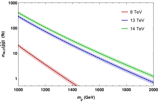
Figure 2: Gluino pair production cross section at the LHC for $\sqrt{s}=8,13,14$ TeV calculated at NLO with Prospinoprospino . Squarks are assumed to be heavy with mass $m_{\tilde{q}}=5$ TeV. The shaded areas show the scale uncertainty.

III.2 Gluino branching fractions and signatures

Once produced, the gluinos can cascade decaycascade to a variety of final states which are listed in Table 2. The decay modes including $q$ in the final state are summed over $q=u,d,s,c$ possibilities. It is evident from the Table that in all cases the decays to third generation quarks are enhanced over first/second generation quarks. Gluino three-body decays to third generation quarks were first calculated in Ref’s btw ; bartl ; btw2 where their enhancement was noticed to arise from 1. couplings which include the large $b$ and $t$ Yukawa couplings, 2. generically smaller mediator masses $m_{\tilde{t}_{1,2}}\lesssim m_{\tilde{q}}$ and 3. large L-R mixing effects. For our benchmark models, we see that in mSUGRA, the $\tilde{g}$ decays to states including $b\bar{b}$ (both directly and via decay to top followed by $t\rightarrow bW$) 81% of the time, while for CSB it is 47% and for RNS it is 99.1%. Thus, for $\tilde{g}\tilde{g}$, we usually expect the presence of four $b$-jets in the final state (although some of these may fall below acceptance cuts or be merged with other $b$-jets etc.). In the CSB case, the branching to $t$ and $b$ quarks is only mildly enhanced since all six squark flavors are extremely heavy. In addition, in the mSUGRA and CSB cases, gluinos only decay substantially to the lighter -ino states $\widetilde{W}_{1}$ and $\widetilde{Z}_{1,2}$. For the RNS case, gluino decays to the light higgsino-like EWinos dominates but also decays to the heavier bino- and wino-like states $\widetilde{Z}_{3,4}$ and $\widetilde{W}_{2}$ can be substantial.

final state	mSUGRA	CSB	RNS
$q\bar{q}^{\prime}\tilde{W}_{1}$	10.5 %	34.0 %	0.1 %
$tb\tilde{W}_{1}$	13.4 %	28.8 %	45.6 %
$tb\tilde{W}_{2}$	– %	– %	2.2 %
$q\bar{q}\tilde{Z}_{1}$	3.1 %	17.0 %	– %
$b\bar{b}\tilde{Z}_{1}$	0.5 %	8.7 %	– %
$t\bar{t}\tilde{Z}_{1}$	60.3 %	6.2 %	17.2 %
$q\bar{q}\tilde{Z}_{2}$	5.2 %	2.4 %	– %
$b\bar{b}\tilde{Z}_{2}$	4.3 %	0.3 %	– %
$t\bar{t}\tilde{Z}_{2}$	2.5 %	3.0 %	22.5 %
$t\bar{t}\tilde{Z}_{3}$	– %	– %	10.6 %
$t\bar{t}\tilde{Z}_{4}$	– %	– %	1.0 %

Table 2: Gluino branching fractions for the three benchmark models where $q=u$, $d$, $c$ and $s$.

A diagram depicting gluino pair production followed by typical three-body decays is shown in Fig. 3. The presence of up to four $b$-jets in the final state can be used as a powerful veto against dominant SM backgrounds such as $t\bar{t}$ production. Indeed, ATLAS searchesatlas_b for $\tilde{g}\tilde{g}$ production with $\geq 3$ $b$-jets in the final state offers the most powerful probe of gluino masses in the case where $m_{\tilde{g}}\ll m_{\tilde{q}}$.

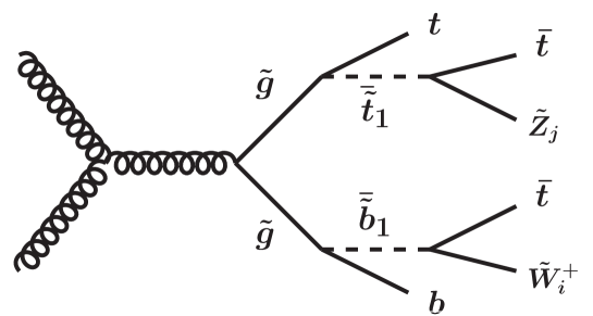
Figure 3: Gluino pair production and decay to multiple $b$-jets in the three benchmark scenarios.

III.3 Gluino cascade decay signatures

We use Isajet 7.84isajet to generate a SUSY Les Houches Accordlha (SLHA) file for each benchmark scenario which is fed into Pythiapythia for generation of gluino pair production events followed by cascade decays. The gluino pair cross section is normalized to the NLO Prospino results of Fig. 2. We use the Snowmass SM background event setAvetisyan:2013onh for the background processes. The $t\bar{t}$ background set is expected to be the dominant backgroundgabe , where extra $b$-jets can arise from initial/final state radiation and from jet mis-tags. While the Snowmass background set was generated for $\sqrt{s}=14$ TeV LHC collisions, we have re-scaled the rates for $\sqrt{s}=13$ TeV collisions. Our signal and BG events are passed through the Delphesdelphes toy detector simulation as set up for Snowmass analyses.

We apply the following event selection cuts:

• $n(\textit{jets})\geq 4$ ,

• $n(\textit{b-jets})\geq 3$,

• $E_{T}(j_{1},j_{2-4})>100,50\,\textrm{GeV}$,

• for isolated leptons, then $p_{T}(\ell)>20\,\textrm{GeV}$,

• $\not{E}_{T}>\not{E}_{T}(cut)=50,100-500\,\textrm{GeV}$

• $A_{T}>1200\,\textrm{GeV}$,

where $A_{T}=\not{E}_{T}+\sum_{leptons}E_{T}+\sum_{jets}E_{T}$ and for later use $M_{\textrm{eff}}=\not{E}_{T}+\sum_{i=1}^{4}E_{T}(j_{i})$. To gain some optimization of signal-to-background (S/B), we tried the above range of $\not{E}_{T}$ cuts and evaluated S/B with and without the $A_{T}$ cut.

The cross sections after cuts for various multi-lepton $+\geq 3$ $b$-jets + $\not{E}_{T}$ channels are shown in Fig. 4. The optimal $\not{E}_{T}$ cut for the $0\ell$ and $1\ell$ channels was the hardest value: $\not{E}_{T}>500$ GeV. For the Opposite Sign Same Flavor (OSSF) dilepton channel, the best cut was $\not{E}_{T}>400$ GeV while for the Same Sign ($SS$)-dilepton, $3\ell$ and $4\ell$ channels, the $\not{E}_{T}>50$ GeV was best. The $A_{T}>1200$ GeV cut helped just marginally.

We see, from Fig. 4, that the signal cross sections after cuts in the jets$+\not{E}_{T}$ ($0\ell$) channel are 1.9, 3.3 and 2.1 fb repectively for the mSUGRA, CSB and RNS cases while SM BG lies at 1.2 fb. In Fig. 5, we show the required value of LHC13 integrated luminosity which is needed to establish a $5\sigma$ signal, where in addition we also require at least 10 total signal events. From this plot, we see that just 8.3, 3.1 or 6.9 fb^-1 of integrated luminosity $L$ is needed to establish a first signal for the mSUGRA, CSB and RNS benchmark models with $m_{\tilde{g}}=1.4$ TeV. The CSB benchmark model has a somewhat larger signal cross section and hence requires somewhat lower $L$ in the $0\ell$ channel as compared to the mSUGRA and RNS models since its decay modes include more hadronic and fewer leptonic cascades.

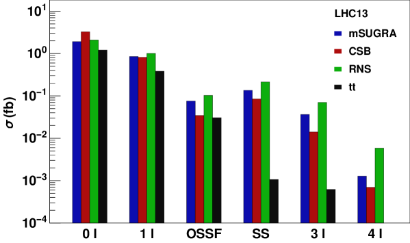
Figure 4: Cross section after cuts from gluino pair production for the three SUSY benchmark models and from $t\bar{t}$ background. For the $0$ and $1\ell$ signals, we take $\not{E}_{T}>500$ GeV while for the OSSF dilepton channel we take $\not{E}_{T}>400$ GeV. For the SS, $3\ell$ and $4\ell$ signals, we require $\not{E}_{T}>50$ GeV.

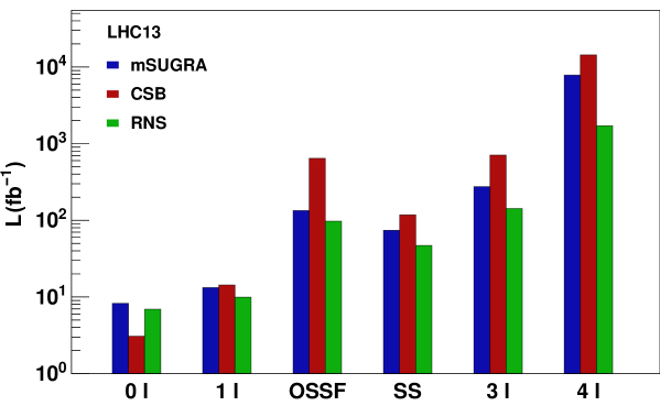
Figure 5: Required integrated luminosity at LHC13 to establish a $5\sigma$ SUSY discovery in various channels from gluino pair production for the three SUSY benchmark models compared to $t\bar{t}$ background. For the $0$ and $1\ell$ signals, we take $\not{E}_{T}>500$ GeV while for the OSSF dilepton channel we take $\not{E}_{T}>400$ GeV. For the SS, $3\ell$ and $4\ell$ signals, we require $\not{E}_{T}>50$ GeV.

In Fig. 4, we also see the cross section after cuts for the $1\ell$ channel. Even though one takes a leptonic branching fraction hit in this channel, the numerous sources for a single additional isolated lepton lead to cross sections after cuts which are comparable to those in the $0\ell$ channel. For the $1\ell$ channel, RNS has the largest cross section $1.0$ fb while mSUGRA and CSB are at the 0.8 fb level. This $1\ell+jets+\not{E}_{T}$ channel will confirm the signal which is already established in the $0\ell$ channel with just a few additional (10-14) fb^-1 of integrated luminosity.

In Fig. 4 and 5, we also show the cross section after cuts and the required integrated luminosity for a $5\sigma$ signal for the OSSF, SS, $3\ell$ and $4\ell$ channels. These multi-lepton channels all exhibit a greater suppression due to multiple leptonic branching fractions as compared to the $0\ell$ channel. For the $3\ell$ channel, background events come from isolated leptons in the $b$-quark decays. With the requirement of at least 3 $b$-jets, we do not observe any events in our $t\bar{t}$ background for the $4\ell$ channel. Also, in the multi-lepton channels, we see that the RNS model yields the largest cross sections due to the large gluino branching fractions into tops followed by $t\rightarrow bW$ and $W\rightarrow\ell\nu$ decay. From Fig. 5, we see that typically $\sim 100$ fb^-1 is necessary to establish a signal in the dilepton and trilepton channels while $\sim 10^{3}-10^{4}$ fb^-1 would be required for a $5\sigma$ signal in the $4l$ channel.

IV Establishing the LSP archetype

IV.1 Charged SUSY breaking

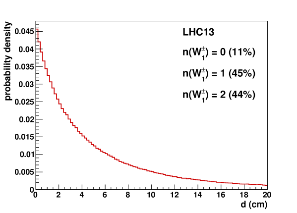
Figure 6: Distance to the decay point from the interaction vertex for the CSB benchmark model.

One of the features of the CSB model is that $\tilde{W}_{1}$ and the LSP are almost degenerate with a mass difference $\Delta m=m_{\tilde{W}_{1}}-m_{\tilde{Z}_{1}}\gtrsim m_{\pi^{\pm}}$. $\tilde{W}_{1}$ decays into charged pions at almost 100% rate. The reduced phase space also makes the chargino long-lived so that, once produced at the interaction vertex, it travels a visible distance before it decays to soft pions plus the LSP. Since the chargino is so massive, its velocity is borderline relativistic leading to a highly-ionizing trail or track (HIT). The chargino lifetime $\tau_{\widetilde{W}_{1}}$ is extracted from Isajet and the actual lifetime of each chargino is generated from the exponential decay law $e^{-t/\tau_{\widetilde{W}_{1}}}$. Then the track length is computed from $d=\beta\gamma t$.

In Figure 6, we display the histogram of the distance travelled from the interaction vertex to the decay point of each chargino. Here, we see that the typical length of each HIT is of order 2-20 cm. We also display the percentage of events containing 0-2 charginos. We see that 90% of the events passing our cuts contain either one or two charginos in each event. The presence of one-or-more HITs in candidate SUSY events would be the smoking gun signature of SUSY models with a wino-like LSP.

IV.2 Radiatively-driven naturalness (RNS)

In the RNS benchmark model, it is emphasizedbbh ; ltr ; rns@lhc that the mass gap between the $\widetilde{Z}_{2}$ and $\widetilde{Z}_{1}$ neutralinos is typically small: $\sim 10-30$ GeV which gives the inter-higgsino splitting. For our benchmark case, the value is $\Delta m=m_{\tilde{Z}_{2}}-m_{\tilde{Z}_{1}}=27.4$ GeV. Notice this mass gap never gets much below about 10 GeV since naturalness also provides upper bounds to the gaugino masses via loop effects so that the higgsino-gaugino mass gap cannot become arbitrarily large. The modest $\widetilde{Z}_{2}-\widetilde{Z}_{1}$ mass gap has important consequences for phenomenology. It means that the $\widetilde{Z}_{2}$ always decays via $3$-body modes $\widetilde{Z}_{2}\rightarrow\widetilde{Z}_{1}f\bar{f}$ which is dominated by $Z^{*}$ exchange. The decay mode $\widetilde{Z}_{2}\rightarrow\widetilde{Z}_{1}\ell^{+}\ell^{-}$ occurs at 3-4% per lepton species, but the OSSF dilepton pair which emerges from this decay always has invariant mass kinematically bounded by $m_{\widetilde{Z}_{2}}-m_{\widetilde{Z}_{1}}$. This mass edge should be apparent in gluino pair cascade decay events which contain an OSSF dilepton pair.

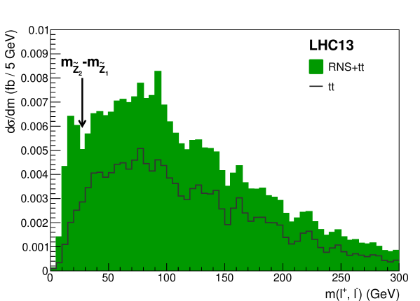
Figure 7: Invariant mass of OSSF leptons. The dilepton mass edge and the $Z$ peak are visible for the RNS model. We require $n(\textit{b-jets})\geq 3$.

In Fig. 7, we show the invariant mass distribution of OSSF dilepton pairs in gluino pair cascade decay events where we require the above cuts but with $\not{E}_{T}>\max(100\ {\rm GeV},0.2M_{eff})$ and $A_{T}>1200$ GeV and the presence of an isolated OSSF dilepton pair. The black histogram shows the expected continuum background distribution arising mainly from $t\bar{t}$ production while the green histogram shows signal plus BG for the RNS benchmark model. The RNS signal is characterized by the distinct mass bump and edge below about 30 GeV. This feature provides the smoking gun signature for SUSY models with light higgsinosrns@lhc . One can also see a peak at $m(\ell^{+}\ell^{-})\sim m_{Z}$ which arises from $\widetilde{W}_{2}$ and $\widetilde{Z}_{3,4}$ two-body decays to a real $Z$. The area under the $m(\ell^{+}\ell^{-})<30$ GeV portion is $\sim 0.025$ fb so that of order 400 fb^-1 of integrated luminosity will be required before this feature begins to take shape in real data.

For comparison, in Fig. 8 we show the same $m(\ell^{+}\ell^{-})$ distribution for the case of the CSB benchmark. In the CSB case, first of all there are far fewer $\ell^{+}\ell^{-}$ pairs present above background, and second there is no obvious structure to the signal distribution: we expect just a continuum.

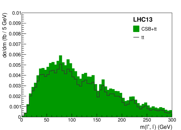
Figure 8: Invariant mass of OSSF dileptons for the CSB model. We require $n(\textit{b-jets})\geq 3$.

The second smoking gun signature for models with a higgsino LSP is the presence of same-sign diboson (SSdB) events which are from wino pair productionlhcltr ; rns@lhc . In this case, the production reaction is typically $pp\rightarrow\widetilde{W}_{2}\widetilde{Z}_{4}$ followed by $\widetilde{W}_{2}\rightarrow\widetilde{W}_{1}\widetilde{Z}_{1,2}$ and $\widetilde{Z}_{4}\rightarrow\widetilde{W}_{1}^{\pm}W^{\mp}$. The Majorana nature of the $\widetilde{Z}_{4}$ leads to equal amounts of same-sign and opposite sign dilepton events. Note that these SSdB events contain minimal jet activity– only that arising from initial state QCD radiation– as opposed to SS dilepton events from gluino and squark cascade decays which should be rich in the presence of additional high $p_{T}$ jets.

IV.3 mSUGRA/CMSSM

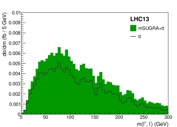
Figure 9: Invariant mass of OSSF dileptons for the mSUGRA model. We require $n(\textit{b-jets})\geq 3$.

For the mSUGRA/CMSSM benchmark model with a 1.4 TeV gluino, then we expect the production of the usual multi-lepton+multi-jet + $\not{E}_{T}$ cascade decay signatures as shown in Fig. 4. For the case of the mSUGRA benchmark, the mass gap between the wino-like $\widetilde{Z}_{2}$ and the bino-like $\widetilde{Z}_{1}$ is 225.5 GeV so that the $\widetilde{Z}_{2}\rightarrow\widetilde{Z}_{1}h$ (spoiler) decay mode is open. This two-body decay dominates the $\widetilde{Z}_{2}$ branching fraction and so we expect no additional structure in the dilepton invariant mass distribution. The $m(\ell^{+}\ell^{-})$ distribution for the mSUGRA benchmark point is shown in Fig. 9. While no characteristic dilepton structure is apparent, it may be possible instead to pull out the presence of $h\rightarrow b\bar{b}$ decays in the mSUGRA cascade decay events where $m(b\bar{b})\sim m_{h}$oldhbb .

V Conclusions

During run 1 of the LHC at $\sqrt{s}=7-8$ TeV, the Standard Model was vigorously confirmed in both the electroweak and QCD sectors and the Higgs boson was discovered at $m_{h}\simeq 125$ GeV. The presence of a bonafide fundamental scalar particle cries out for a mass stabilization mechanism of which the simplest and most elegant one is supersymmetry. Unfortunately, no SUSY particles have yet appeared leading to mass limits for the gluino particle of $m_{\tilde{g}}\gtrsim 1.3$ TeV.

LHC Run 2 with $\sqrt{s}=13$ TeV has begun! New vistas in SUSY parameter space are open for exploration. While naturalness allows for gluinos as high as 4-5 TeV (with $\Delta_{EW}<30$), it is yet true that naturalness (mildly via higher order contributions) prefers gluinos as light as possible. Motivated by these circumstances, we considered how SUSY discovery would unfold in three SUSY archetype models with a bino-, wino- and higgsino-like LSP each with a 1.4 TeV gluino, just beyond present bounds.

We find that SUSY discovery could already arise at the $5\sigma$ level with just $3-8$ fb^-1 of integrated luminosity via the $\geq 3\ b-{\rm jet}+\not{E}_{T}$ channel. Confirmation would soon follow in the $\geq 3\ b-{\rm jet}+1-\ell+\not{E}_{T}$ channel. Further confirmation in the 2-3 lepton channels will require $\sim 100$ fb^-1. The CSB benchmark case would immediately be identified by the presence of one or more highly ionizing tracks in each signal event due to long-lived wino-like charginos which undergo delayed decays to a wino-like LSP. No such HITs should be apparent in signal events from the mSUGRA or RNS archetype models. Instead, the RNS archtype would be signalled by a gradual buildup of structure in the $m(\ell^{+}\ell^{-})$ OSSF dilepton mass distribution, where the $m(\ell^{+}\ell^{-})<m_{\widetilde{Z}_{2}}-m_{\widetilde{Z}_{1}}$ mass edge along with a $Z$ peak should be apparent with $\sim 100-1000$ fb^-1. In the RNS case, the gluino cascade decay events should ultimately be accompanied by the presence of same-sign diboson events arising from wino pair production.

For the mSUGRA archtype with a bino-like LSP, then we expect the usual assortment of gluino-pair-initiated cascade decay multilepton+jets + $\not{E}_{T}$ events but without HITs and without any apparent structure in the $m(\ell^{+}\ell^{-})$ distribution. However, the presence of Higgs bosons lurking within the cascade decay events may be a distinguishing feature. On to data from LHC13!

- (1) I. Hinchliffe, talk at Pheno 2015 meeting, PITTPAC, Pittsburgh, May 2015.
- (2) G. Aad et al. [ATLAS Collaboration], Phys. Lett. B716 (2012) 1.
- (3) S. Chatrchyan et al. [CMS Collaboration], Phys. Lett. B716 (2012) 30.
- (4) J. Lykken and M. Spiropulu, Sci. Am. 310N5 (2014) 5, 36.
- (5) M. S. Carena and H. E. Haber, Prog. Part. Nucl. Phys. 50 (2003) 63.
- (6) H. Baer, V. Barger and A. Mustafayev, Phys. Rev. D 85 (2012) 075010.
- (7) A. Arbey, M. Battaglia, A. Djouadi, F. Mahmoudi and J. Quevillon, Phys. Lett. B 708 (2012) 162.
- (8) H. P. Nilles, Phys. Lett. B 115 (1982) 193; A. Chamseddine, R. Arnowitt and P. Nath, Phys. Rev. Lett. 49 (1982) 970; R. Barbieri, S. Ferrara and C. Savoy, Phys. Lett. B119 (1982) 343; N. Ohta, Prog. Theor. Phys. 70, 542 (1983); L. Hall, J. Lykken and S. Weinberg, Phys. Rev. D27 (1983) 2359; for an early review, see e.g. H. P. Nilles, Phys. Rept. 110 (1984) 1; for a recent review, see D. J. H. Chung, L. L. Everett, G. L. Kane, S. F. King, J. D. Lykken and L. T. Wang, Phys. Rept. 407 (2005) 1.
- (9) R. Arnowitt, A. H. Chamseddine and P. Nath, Int. J. Mod. Phys. A 27 (2012) 1230028; see also P. Nath, arXiv:1502.00639 [physics.hist-ph]; H. P. Nilles, Nucl. Phys. Proc. Suppl. 101 (2001) 237.
- (10) H. Baer, V. Barger, P. Huang, A. Mustafayev and X. Tata, Phys. Rev. Lett. 109 (2012) 161802.
- (11) H. Baer, V. Barger, P. Huang, D. Mickelson, A. Mustafayev and X. Tata, Phys. Rev. D 87 (2013) 115028.
- (12) H. Baer, V. Barger and D. Mickelson, Phys. Rev. D 88 (2013) 095013.
- (13) H. Baer, V. Barger, D. Mickelson and M. Padeffke-Kirkland, Phys. Rev. D 89 (2014) 115019.
- (14) H. Baer, V. Barger and M. Savoy, Phys. Scripta 90 (2015) 6, 068003 [arXiv:1502.04127 [hep-ph]].
- (15) J. R. Ellis, K. Enqvist, D. V. Nanopoulos and F. Zwirner, Mod. Phys. Lett. A 1 (1986) 57.
- (16) R. Barbieri and G. F. Giudice, Nucl. Phys. B 306 (1988) 63.
- (17) D. Matalliotakis and H. P. Nilles, Nucl. Phys. B 435 (1995) 115; P. Nath and R. L. Arnowitt, Phys. Rev. D 56 (1997) 2820; J. Ellis, K. Olive and Y. Santoso, Phys. Lett. B539 (2002) 107; J. Ellis, T. Falk, K. Olive and Y. Santoso, Nucl. Phys. B652 (2003) 259; H. Baer, A. Mustafayev, S. Profumo, A. Belyaev and X. Tata, JHEP0507 (2005) 065.
- (18) H. Baer, V. Barger, A. Lessa and X. Tata, Phys. Rev. D 86 (2012) 117701.
- (19) H. Baer, V. Barger, P. Huang, D. Mickelson, A. Mustafayev, W. Sreethawong and X. Tata, JHEP 1312 (2013) 013.
- (20) F. E. Paige, S. D. Protopopescu, H. Baer and X. Tata, hep-ph/0312045.
- (21) G. G. Ross and R. G. Roberts, Nucl. Phys. B 377, 571 (1992).
- (22) R. L. Arnowitt and P. Nath, Phys. Rev. Lett. 69, 725 (1992).
- (23) V. D. Barger, M. S. Berger and P. Ohmann, Phys. Rev. D 47, 1093 (1993) [hep-ph/9209232].
- (24) V. D. Barger, M. S. Berger and P. Ohmann, Phys. Rev. D 49, 4908 (1994) [hep-ph/9311269].
- (25) L. Randall and R. Sundrum, Nucl. Phys. B 557, 79 (1999); G. F. Giudice, M. A. Luty, H. Murayama and R. Rattazzi, JHEP 9812, 027 (1998).
- (26) T. Gherghetta, G. F. Giudice and J. D. Wells, Nucl. Phys. B 559 (1999) 27; J. L. Feng, T. Moroi, L. Randall, M. Strassler and S. f. Su, Phys. Rev. Lett. 83 (1999) 1731.
- (27) H. Baer, V. Barger and A. Mustafayev, JHEP 1205 (2012) 091.
- (28) J. D. Wells, hep-ph/0306127; J. D. Wells, Phys. Rev. D 71, 015013 (2005).
- (29) N. Arkani-Hamed and S. Dimopoulos, JHEP 0506, 073 (2005); G. F. Giudice and A. Romanino, Nucl. Phys. B 699, 65 (2004) [Erratum-ibid. B 706, 65 (2005)]; N. Arkani-Hamed, S. Dimopoulos, G. F. Giudice and A. Romanino, Nucl. Phys. B 709, 3 (2005).
- (30) M. Ibe and T. T. Yanagida, Phys. Lett. B 709, 374 (2012); M. Ibe, S. Matsumoto and T. T. Yanagida, Phys. Rev. D 85, 095011 (2012); B. Bhattacherjee, B. Feldstein, M. Ibe, S. Matsumoto and T. T. Yanagida, Phys. Rev. D 87, 015028 (2013); J. L. Evans, M. Ibe, K. A. Olive and T. T. Yanagida, Eur. Phys. J. C 73, 2468 (2013); J. L. Evans, M. Ibe, K. A. Olive and T. T. Yanagida, Eur. Phys. J. C 74, 2931 (2014); J. L. Evans, M. Ibe, K. A. Olive and T. T. Yanagida, arXiv:1412.3403 [hep-ph].
- (31) L. J. Hall and Y. Nomura, JHEP 1201, 082 (2012); L. J. Hall, Y. Nomura and S. Shirai, JHEP 1301, 036 (2013).
- (32) M. Dine, A. Kagan and S. Samuel, Phys. Lett. B 243, 250 (1990); A. Cohen, D. B. Kaplan and A. Nelson, Phys. Lett. B 388, 588 (1996); N. Arkani-Hamed and H. Murayama, Phys. Rev. D 56, 6733 (1997); T. Moroi and M. Nagai, Phys. Lett. B 723, 107 (2013).
- (33) H. Baer, C. Balazs and A.Belyaev, JHEP 0203, 042 (2002).
- (34) T. Moroi and L. Randall, Nucl. Phys. B 570, 455 (2000).
- (35) K. J. Bae, H. Baer, A. Lessa and H. Serce, arXiv:1502.07198 [hep-ph].
- (36) M. Dine, W. Fischler and M. Srednicki, Phys. Lett. B104 (1981) 199; A. P. Zhitnitskii, Sov. J. Phys. 31 (1980) 260.
- (37) E. J. Chun, Phys. Rev. D 84 (2011) 043509; K. J. Bae, E. J. Chun and S. H. Im, JCAP 1203 (2012) 013; K. J. Bae, H. Baer and E. J. Chun, JCAP 1312, 028 (2013).
- (38) H. Murayama, H. Suzuki and T. Yanagida, Phys. Lett. B 291 (1992) 418; T. Gherghetta and G. L. Kane, Phys. Lett. B 354 (1995) 300; K. Choi, E. J. Chun and J. E. Kim, Phys. Lett. B 403 (1997) 209.
- (39) K. J. Bae, H. Baer and H. Serce, Phys. Rev. D 91 (2015) 015003.
- (40) K. J. Bae, H. Baer and E. J. Chun, Phys. Rev. D 89 (2014) 031701.
- (41) H. Baer, V. Barger, P. Huang, D. Mickelson, M. Padeffke-Kirkland and X. Tata, Phys. Rev. D 91, no. 7, 075005 (2015).
- (42) I. Affleck and M. Dine, Nucl. Phys. B 249 (1985) 361.
- (43) M. Dine, L. Randall and S. D. Thomas, Phys. Rev. Lett. 75 (1995) 398; M. Dine, L. Randall and S. D. Thomas, Nucl. Phys. B 458 (1996) 291.
- (44) W. Beenakker, R. Hopker and M. Spira, hep-ph/9611232.
- (45) H. Baer, J. R. Ellis, G. B. Gelmini, D. V. Nanopoulos and X. Tata, Phys. Lett. B 161 (1985) 175; G. Gamberini, Z. Phys. C 30 (1986) 605; H. Baer, V. D. Barger, D. Karatas and X. Tata, Phys. Rev. D 36 (1987) 96; H. Baer, R. M. Barnett, M. Drees, J. F. Gunion, H. E. Haber, D. L. Karatas and X. R. Tata, Int. J. Mod. Phys. A 2 (1987) 1131; R. M. Barnett, J. F. Gunion and H. E. Haber, Phys. Rev. D 37 (1988) 1892. H. Baer, A. Bartl, D. Karatas, W. Majerotto and X. Tata, Int. J. Mod. Phys. A 4 (1989) 4111;
- (46) H. Baer, X. Tata and J. Woodside, Phys. Rev. D 42 (1990) 1568.
- (47) A. Bartl, W. Majerotto, B. Mosslacher, N. Oshimo and S. Stippel, Phys. Rev. D 43 (1991) 2214; A. Bartl, W. Majerotto and W. Porod, Z. Phys. C 64 (1994) 499.
- (48) H. Baer, C. h. Chen, M. Drees, F. Paige and X. Tata, Phys. Rev. D 58 (1998) 075008.
- (49) G. Aad et al. [ATLAS Collaboration], JHEP 1410 (2014) 24.
- (50) P. Z. Skands, B. C. Allanach, H. Baer, C. Balazs, G. Belanger, F. Boudjema, A. Djouadi and R. Godbole et al., JHEP 0407 (2004) 036.
- (51) T. Sjostrand, S. Mrenna and P. Z. Skands, JHEP 0605 (2006) 026.
- (52) A. Avetisyan, J. M. Campbell, T. Cohen, N. Dhingra, J. Hirschauer, K. Howe, S. Malik and M. Narain et al., arXiv:1308.1636 [hep-ex].
- (53) H. Baer, V. Barger, G. Shaughnessy, H. Summy and L. t. Wang, Phys. Rev. D 75 (2007) 095010.
- (54) J. de Favereau et al. [DELPHES 3 Collaboration], JHEP 1402 (2014) 057.
- (55) H. Baer, V. Barger and P. Huang, JHEP 1111 (2011) 031.
- (56) H. Baer, V. Barger, P. Huang, D. Mickelson, A. Mustafayev, W. Sreethawong and X. Tata, Phys. Rev. Lett. 110 (2013) 15, 151801.
- (57) H. Baer, M. Bisset, X. Tata and J. Woodside, Phys. Rev. D 46 (1992) 303. H. Baer, C. h. Chen, F. Paige and X. Tata, Phys. Rev. D 52 (1995) 2746.