A Tool for Computing and Estimating the Volume of the Solution Space of SMT(LA) Constraints

Abstract

There are already quite a few tools for solving the Satisfiability Modulo Theories (SMT) problems. In this paper, we present VolCE, a tool for counting the solutions of SMT constraints, or in other words, for computing the volume of the solution space. Its input is essentially a set of Boolean combinations of linear constraints, where the numeric variables are either all integers or all reals, and each variable is bounded. The tool extends SMT solving with integer solution counting and volume computation/estimation for convex polytopes. Effective heuristics are adopted, which enable the tool to deal with high-dimensional problem instances efficiently and accurately.

1 Introduction

In recent years, there have been a lot of works on solving the Satisfiability Modulo Theories (SMT) problem. Quite efficient SMT solvers have been developed, such as CVC3, MathSAT, Yices and Z3. In [13], we studied the counting version of SMT solving, and presented some techniques for computing the size of the solution space efficiently. This problem can be regarded as an extension to SMT solving, and also an extension to model counting in the propositional logic. It has recently gained much attention in the software engineering community [11, 9].

The prototype tool presented in [13] computes the exact volume of solution space. However, exact volume computation in general is an extremely difficult problem. It has been proved to be #P-hard, even for explicitly described polytopes. On the other hand, it suffices to have an approximate value of the volume in many cases. Recently we implemented a tool to estimate the volume of polytopes; and integrated it into the framework of [13].

This paper presents the new tool VolCE for the counting version of SMT(LA). (Here LA stands for linear arithmetic.) The input of the tool is a set of Boolean combinations of linear constraints, where each numeric variable is bounded. Independent Boolean variables may also appear in the constraints. The output of the tool is the “volume” of the solution space, or the number of solutions in case that the domain consists of integer points.

The rest of this paper is organized as follows. Section 2 presents the architecture of VolCE. Section 3 presents the algorithm and implementation of our volume estimation sub-procedure. Section 4 briefly describes how to use the tool. Section 5 discusses our experiments, and Section 6 describes some related works. We conclude in Section 7.

2 Architecture of VolCE

The architecture of VolCE is illustrated in Figure 1. Recall that in [13], a consistent conjunction of linear constraints that satisfies the boolean skeleton of the SMT(LA) formula is called a feasible assignment. The sum of volumes of all feasible assignments is the volume of the whole formula. In VolCE, the SAT solving engine (MiniSat) and the linear arithmetic solver (lp_solve) work together to find feasible assignments. Each time a feasible assignment is obtained, VolCE tries to reduce it to a partial assignment that still propositionally satisfies the formula. The resulted feasible partial assignment may cover a bunch of feasible assignments, hence is called a “bunch”. Then a solution counting or volume computation/estimation sub-procedure is called for the polytope corresponding to each bunch rather than each feasible assignment, so that the number of calls is reduced. For more details of the main algorithm, see [13].

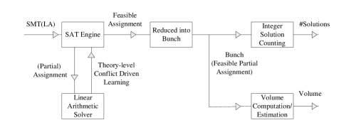
Figure 1: The Architecture of VolCE

In addition to MiniSat and lp_solve, VolCE calls Vinci [3] and LattE [5] to help compute the size of the solution space. Vinci is a tool for computing the volume of a convex body. LattE is a tool for counting lattice points inside convex polytopes and solutions of integer programs. Moreover, we implemented a tool for estimating the volume of convex polytopes, called PolyVest [8]. It will be elaborated in the subsequent section.

3 Volume Estimation

The performance of volume computation packages for convex polytopes is the bottleneck of the prototype tool in [13]. Recently we augmented it with an efficient volume estimation sub-procedure for convex polytopes.

3.1 Volume Estimation for Convex Polytopes

A straightforward way to estimate the volume of a convex body is the Monte-Carlo method. However, it suffers from the curse of dimensionality, which means the possibility of sampling inside a certain space in the target object decreases very quickly while the dimension increases. As a result, the sample size has to grow exponentially to achieve a reasonable estimation. To avoid the curse of dimensionality, Dyer et.al. proposed a polynomial time randomized approximation algorithm (Multiphase Monte-Carlo Algorithm) [6]. The theoretical complexity of the original algorithm is $O^{*}(n^{23})$, and is recently reduced to $O^{*}(n^{4})$ [12].

Based on the Multiphase Monte-Carlo method, we implemented our own tool PolyVest (Polytope Volume Estimation) to estimate the volume of convex polytopes [8]. One improvement over the original Multiphase Monte-Carlo method is that we developed a new technique to reutilize sample points, so that the number of sample points can be significantly reduced.

In the sequel, we briefly describe the algorithm implemented in PolyVest. For more details, one can refer to [8]. We assume that $P$ is a full-dimensional and nonempty convex polytope. We use $vol(K)$ to represent the volume of a convex body $K$, and $B(x,R)$ to represent the ball with radius $R$ and center $x$.

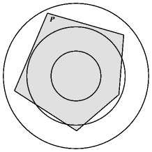
Figure 2: Multiphase Monte-Carlo

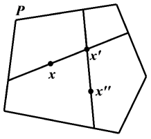
Figure 3: Hit-and-run

The basic procedure of PolyVest consists of the following three steps: rounding, subdivision and sampling.

Rounding  First we find an affine transformation $T$ on polytope $P$ so that $T(P)$ contains the unit ball $B(0,1)$, and is contained in the ball $B(0,r)$. This can be achieved by applying the Shallow-$\beta$-Cut Ellipsoid Method [10]. We set $r=2n$ in our implementation. Rounding is an essential step. For example, it is difficult to subdivide a very “thin” polytope and sample on it without rounding. For simplicity, we still use $P$ to denote the new polytope $T(P)$ after rounding.

Subdivision  Then we divide $P$ into a sequence of convex bodies. The general idea of the subdivision step is illustrated in Figure 3. We place $l$ concentric balls $\{B_{i}\}$ between $B(0,1)$ and $B(0,r)$. Let $K_{i}$ denote the convex body $B_{i}\cap P$, then

$$vol(P)=vol(K_{0})\prod_{i=0}^{l-1}\frac{vol(K_{i+1})}{vol(K_{i})}.$$

Let $\alpha_{i}$ denote the ratio $vol(K_{i+1})/vol(K_{i})$, then

$$vol(P)=vol(K_{0})\prod_{i=0}^{l-1}\alpha_{i}.$$

Hence the volume of the polytope $P$ is transformed to the products of ratios and the volume of $K_{0}$. Note that $K_{0}=B(0,1)$ whose volume can be easily computed. So we only have to estimate the value of $\alpha_{i}$.

Of course, one would like to choose the number of concentric balls, $l$, to be small. However, one needs about $O(l\alpha_{i})$ random points to get a sufficiently good approximation for $\alpha_{i}$. It follows that the $\alpha_{i}$ must not be too large. In PolyVest, we set $l=\lceil n\log_{2}r\rceil$ and $B_{i}=B(0,2^{i/n})$ to construct the convex bodies $\{K_{i}\}$. And it can be proved that $1\leq\alpha_{i}\leq 2$ with this construction.

Sampling  Finally, we generate $S$ points in $K_{i+1}$ and count the number of points $c_{i}$ in $K_{i}$. Thus $\alpha_{i}$ can be approximated with $S/c_{i}$. Generating independent uniformly distributed random points in $\{K_{i}\}$ is not as simple as in cubes or ellipsoids. So we use a hit-and-run method for sampling. Hit-and-run method is a random walk which can generate points with almost uniform distribution in polynomial time [1]. Figure 3 illustrates the hit-and-run method: It starts from a point $x$, then randomly selects a line $L$ through $x$ and choose the next point $x^{\prime}$ uniformly on the segment in $P$ of line $L$. PolyVest adopts the coordinate directions hit-and-run method, in which the random direction of line $L$ is chosen with equal probability from the coordinate direction vectors and their negations.

Reutilization of Sample Points  In the original Multiphase Monte Carlo method, the ratios $\alpha_{i}$ are estimated in natural order, from the first ratio $\alpha_{0}$ to the last one $\alpha_{l-1}$. And the method starts sampling from the origin. However, our implementation works in the opposite way. It generates sample points from the outermost convex body $K_{l}$ to the innermost convex body $K_{0}$, and the ratios are estimated accordingly in reverse order.

The advantage of approximation in reverse order is that it is possible to fully exploit the sample points generated in the previous phases. Since $K_{0}\subseteq K_{1}\subseteq\dots\subseteq K_{l}$, the sample points in $K_{i}$ still fall in $K_{j}$ ($i\leq j$). On the other hand, the sample points generated by the hit-and-run method are almost independent as sample size $S$ is large enough. Therefore, for any $i$ that $i\leq j$, the points generated for approximating $\alpha_{j}$ that hit $K_{i+1}$ can serve as sample points to approximate $\alpha_{i}$ as well. It can be easily proved that we only need to generate less than half sample points with this technique since $\alpha_{i}\leq 2$. In practice, this technique can save over 70% time consumption under most circumstances.

3.2 Volume Estimation for SMT(LRA) Formula

Now we describe how to estimate the “volume” of the solution space of SMT(LRA) formulas. (Here LRA stands for linear real arithmetic.) The basic procedure is quite similar to that of volume computation as described in [13]. As in [13], a consistent conjunction of linear constraints that satisfies the boolean skeleton of the SMT(LRA) formula is called a feasible (partial) assignment. Each time VolCE obtains a feasible (partial) assignment, it calls PolyVest to estimate the volume of the polytope corresponding to this assignment. The sum of estimated volumes of all feasible (partial) assignments is approximately the volume for the whole formula. Note that the “volume computation in bunches” strategy in [13] can also be applied in volume estimation.

In the Multiphase Monte-Carlo method, the number of sample points at each phase is a key parameter. As the sample size increases, the accuracy of estimation improves, and the estimation process also takes more time. It is important to balance the accuracy and run time, especially for VolCE since the estimation subroutine PolyVest is usually called many times.

VolCE employs a two-round strategy that can dynamically determine a proper sample size for each feasible (partial) assignment. At the first round of estimation, each feasible assignment is sampled with a fixed small number of random points to get a quick and rough estimation. Since the volumes of feasible assignments may vary a lot, intuitively a feasible assignment with relatively larger volume should be estimated with higher accuracy. Hence at the second round, the sample size for each assignment is determined according to its estimated volume from the first round. More specifically, we use the following rule to decide the sample sizes in the second round:

• Suppose the sample size in the first round is $S_{min}$, and the largest sample size in the second round is set to $S_{max}$. Let $V_{max}$ denote the largest estimated volume in the first round, and $V_{i}$ denote the volume of the $i$th feasible assignment estimated in the first round. Then the sample size $S_{i}$ for the $i$th feasible assignment in the second round is:

  $$S_{i}=\frac{2\times S_{max}\times V_{i}}{V_{max}}$$

  If $S_{i}\leq S_{min}$, the $i$th feasible assignment is neglected at the second round, and we use the result from the first round as its estimated volume. If $S_{i}>S_{max}$, then set $S_{i}$ to $S_{max}$.

Through statistical results of substantial experiments, we find that setting $S_{min}$ to $40l$ and $S_{max}$ to $1600l$ ($l=\lceil n\log_{2}r\rceil$) is very effective. It only needs to generate $S_{min}/S_{max}=1/40$ points in extreme cases with this strategy. In practice, it usually saves more than $95\%$ points for random instances.

4 Using the Tool

The input of VolCE is an SMT formula where the theory $T$ is restricted to the linear arithmetic theory. It can be regarded as a Boolean combination of linear inequalities. There are two input formats.

For the first format, the input formula is a Boolean formula $\phi(b_{1},\dots,b_{n})$ in conjunctive normal form (CNF). And each Boolean variable $b_{i}$ can stand for a linear arithmetic constraint (LAC). The whole input file is an extension of the DIMACS format for SAT solving. An alternative input format is SMT-Lib style. Currently, VolCE supports the main features of the “SMT-LIBv2” syntax.

VolCE has several command-line options:

• -V asks the tool to call Vinci to compute the volume.

• -P asks the tool to call PolyVest to approximate the volume.

• -L asks the tool to call LattE to count integer solutions.

• -w=NUMBER specifies the word length of variables in bit-wise representations.

• -maxc=NUMBER sets the maximum sampling coefficient of PolyVest, which is an upper bound.

• -minc=NUMBER sets the minimum sampling coefficient of PolyVest.

For more details about using the tool, see the manual. Here we just give an example to show its application to program analysis.

Example from Program Analysis

In [13], we describe a program called getop() and analyze the execution frequency of its paths. For Path1, its path condition is:

    (NOT ((c = 32) OR (c = 9) OR (c = 10))) AND
    ((c != 46) AND ((c < 48) OR (c > 57)))

Here c is a variable of type char; it can be regarded as an integer variable within the domain [-128..127]. For this path condition, we can compute the number of solutions using VolCE. With option -L (i.e., using LattE), the tool tells us that the constraint has $242$ solutions. (We do not need to use the option -w=8, because the default word length is $8$.) Given that the size of the whole search space is $256$, we conclude that the frequency of executing Path1 is about $0.945$ ($242/256$). This means, if the input string has only one character, most probably, the program will follow this path.

Another path, Path2, has a more complicated path condition (omitted here, due to the lack of space). It involves 3 input variables c0, c1 and c2. Given the second path condition, our tool tells us that the number of solutions is 8085. So the path execution frequency is $8085/(256*256*256)$ which is roughly 0.00048.

5 Experimental Results

In this section, we report some experimental results about our tool. The experiments are performed on a workstation with 3.40GHz Intel Core i7-2600 CPU and 8GB memory. In all experiments, the parameter $S_{max}$ is set to 1600, and $S_{min}$ set to 40. The domain of each numeric variable is set to [-128..127] by default.

Benchmarks

The following instances have been tested.

• Instances generated from static program analysis. We analyzed the following programs:

  • abs: a function which calculates absolute value;

  • findmiddle: a function which finds the middle number among 3 numbers;

  • Space_manage: a program related to space technology;

  • tritype: a program which determines the type of a triangle;

  • calDate: a function which converts the special date into a Julian date;

• Instances from SMT-Lib, including: (1) the QF_LRA benchmarks Arthan, atan; and (2) the QF_LIA benchmarks bignum, simplebitadder, fischer, pigeon-hole, prime_cone.

• Random instances ran_$i$_$c$_$d$: which have $d$ numeric variables, $i$ inequalities and $c$ clauses. They are generated by randomly choosing coefficients of LACs and literals of clauses. The length of each clause is between 3 to 5.

In the following tables, “—” means that the instance takes more than one hour to solve (or the tool runs out of memory).

Table 1: Comparison between Volume Estimation and Computation

					PolyVest		Vinci
Instance	Dims	Ineqs	Clauses	Bunches	Result	Time(s)	Result	Time(s)
abs_0	1	1	1	1	127	0.000	127	0.000
findmiddle_2	3	6	20	2	5369040	0.016	5527125	0.000
findmiddle_3	3	6	20	7	5696270	0.020	5527125	0.004
Space_manage_1	17	3	7	1	2.35e+39	2.6	—	—
Arthan1A-chunk-0015	4	6	16	1	2.64e-3	0.016	2.57e-3	0.002
atan-problem-2- weak-chunk-0200	3	6	19	1	2.71	0.008	2.67	0.014
ran_15_45_7	7	15	45	113	1.84e+15	1.4	1.84e+15	12
ran_20_60_7	7	20	60	254	6.68e+14	2.75	6.74e+14	84
ran_30_90_7	7	30	90	401	4.62e+13	5.9	4.58e+13	802
ran_15_45_8	8	15	45	214	3.58e+17	2.9	3.50e+17	72
ran_20_60_8	8	20	60	480	1.07e+17	6.3	1.09e+17	259
ran_30_90_8	8	30	90	1135	6.73e+16	20.7	—	—
ran_20_60_9	9	20	60	425	1.20e+19	8.3	—	—
ran_20_50_9	9	20	50	691	2.86e+19	11.6	—	—
ran_20_60_10	10	20	60	949	2.51e+22	20.3	—	—

Table 1 shows the results of comparison between volume estimation and computation. “Dims” represents the number of numeric variables in LACs. “Ineqs” represents the number of LACs and also represents the number of boolean variables in the boolean skeleton. “Clauses” represents the number of clauses in the boolean skeleton. “Bunches” represents the number of feasible partial assignments obtained by VolCE and also represents the times of VolCE calling PolyVest or Vinci.

Observe that VolCE with PolyVest is very efficient and the relative errors of approximation are small. When the dimension of instance grows to 8 or larger, VolCE with Vinci often fails to give an answer in one hour or depletes memory. Though “Vinci” has an option to restrict its memory storage, as a tradeoff it will take much more time to solve, and still cannot solve instances within the timeout.

Table 2 shows the results of our tools with two-round strategy on random instances. Column “Sample” represents the average coefficient of the sample size of $S_{i}$. In the original algorithm, this average value always equals to $S=S_{max}=1600$. Values in column “Ratio” are approximation of saved sample points by the two-round strategy. Obviously, the two-round strategy could save much time without losing much accuracy. The differences of the results between original and two-round strategy are usually less than 5%. Besides, the two-round strategy could save 93% to 97% sample points and save more than 90% time.

Table 2: Benefits of the Two-Round Strategy

				Original		Two-Round
Dim.	Ineq.	Clause	Bunch	Result	Time(s)	Result	Time(s)	Sample	Ratio
8	15	45	214	3.53e+17	31	3.58e+17	2.9	101.7	93.6%
8	20	60	480	1.10e+17	78.9	1.07e+17	6.3	75.5	95.3%
8	30	90	1135	6.94e+16	210.4	6.73e+16	20.7	54.7	96.6%
10	15	45	228	1.20e+23	68.5	1.20e+23	4.7	63.7	96.0%
10	20	60	949	2.52e+22	312.8	2.51e+22	20.3	61.5	96.2%
10	30	90	1394	8.06e+18	524.6	7.92e+18	39.1	66.0	95.9%
15	40	200	1710	7.93e+27	2958.5	7.94e+27	189.1	44.6	97.2%
15	50	250	495	1.22e+23	984.4	1.23e+23	67.1	48.3	97.0%
20	40	200	8095	—	—	2.08e+40	2283	41.3	97.4%
20	60	400	689	—	—	6.71e+32	285	48.8	97.0%
30	60	400	886	—	—	6.59e+54	1528	44.0	97.3%
40	80	550	451	—	—	6.12e+66	2806	43.5	97.3%

Table 3: Experiments on Larger Instances

Dims	Ineqs	Clauses	Bunches	Result	Time(s)
30	40	200	5200	1.42e+64	4314
30	60	400	886	6.59e+54	1528
30	80	500	610	2.01e+41	1227
40	60	400	1752	5.23e+80	6437
40	80	550	451	6.12e+66	2806
40	100	750	111	5.00e+63	916
50	100	750	24	5.63e+74	650

Table 3 shows the results of experiments with some larger random instances. Note that the number of dimensions and bunches are the key parameters of the scale of instances. The larger the number of dimensions or bunches, the more time the tool has to run. VolCE can handle instances around 30-dimensions in reasonable time and up to 50-dimensions with a few bunches.

Table 4 are the results of counting integer solutions with LattE. It shows that LattE can handle some problems up to 17 dimensions. However, LattE cannot solve the random instance “ran_15_45_7”. The inequalities in the instance are quite complicated.

Table 4: Experiments about counting integer solutions

Instance	Dims	Ineqs	Bunches	Result	Time(s)
abs_0	1	1	1	128	0.000
findmiddle_2	3	6	2	5527040	0.004
tritype_16	4	18	4	8323072	0.051
calDate_13	6	5	1	7.99e+11	0.028
Space_manage_1	17	3	1	2.69e+39	170.3
bignum_lia1	6	13	0	0	0.028
bignum_lia2	6	13	1	0	0.036
SIMPLEBITADDER_2	12	51	98	0	1.3
FISCHER1-1-fair	4	16	1	256	0.020
FISCHER1-2-fair	6	28	0	0	0.004
prime_cone_sat_2	2	5	1	4159	0.004
ran_15_45_7	7	15	45	—	—

6 Related Works

There was little work on the counting of SMT solutions, until quite recently.

Fredrikson and Jha [7] relate a set of privacy and confidentiality verification problems to the so-called model-counting satisfiability problem, and present an abstract decision procedure for it. They implemented this procedure for linear-integer arithmetic. Their tool is called countersat. It is not available to us.

Zhou et al. [18] propose a BDD-based search algorithm which reduces the number of conjunctions. For each conjunction, they propose a Monte-Carlo integration with a ray-based sampling strategy, which approximates the volume. Their tool is named RVC. It can handle formulas with up to 18 variables. But the running time is dozens of minutes.

A different approach is described in [4]. It reduces an approximate version of #SMT to SMT. The approach does not need to modify existing SMT solvers. It has been applied to solve a value estimation problem for certain kind of probabilistic programs. We do not know how large the benchmarks are, and it is not clear about the quality of the approximation.

7 Concluding Remarks

VolCE is a tool for computing and estimating the volume of the solution space (or counting the number of solutions), given a formula/constraint which is a Boolean combination of linear arithmetic inequalities. VolCE is very flexible to use. For medium sized SMT(LA) formulas, it can provide exact volume computation results or exact number of solutions. For larger SMT(LA) formulas, it can quickly perform volume estimation with high accuracy, due to the use of effective heuristics. We believe that the tool will be useful in a number of domains, such as program analysis and probabilistic verification.

Appendix 0.A Introduction of VolCE

0.A.1 What is VolCE?

VolCE is designed for computing or estimating the size of the solution space of an SMT formula where the theory $T$ is restricted to the linear arithmetic theory. (SMT stands for Satisfiability Modulo Theories.) The prototype tool presented in [13] computes the exact volume of the solution space. However, exact volume computation in general is an extremely difficult problem. It has been proved to be #P-hard, even for explicitly described polytopes. On the other hand, it suffices to have an approximate value of the volume in many cases. Later we implemented a tool to estimate the volume of polytopes [8] and integrated it into the framework of [13]. The new tool is called VolCE. It can efficiently handle instances of dozens of dimensions with high accuracy. In addition, VolCE also accepts constraints involving independent Boolean variables.

0.A.2 What can VolCE do?

VolCE uses the following three packages:

• PolyVest [8], which can be used to estimate the volume of polytopes

• Vinci [17], a software package that implements several algorithms for (exact) volume computation.

• LattE (Lattice point Enumeration) [14], a software package dedicated to the problems of counting lattice points and integration inside convex polytopes.

Appendix 0.B Installing VolCE

• Step 1: Make sure that g++ (version 4.8 or higher version) is installed on your machine (you can type “g++ -v” to check this).

• Step 2: The functionality of VolCE is dependent on some other libraries: zlib, boost, lpsolve, glpk, gfortran, LAPACK, BLAS and Armadillo. On Ubuntu or Debian, you can use “apt-cache search” and “apt-get install” to find and install all of these libraries. Or you can download these libraries from:

  Library	URL
  zlib	http://zlib.net/
  boost	http://www.boost.org/
  lpsolve	http://sourceforge.net/projects/lpsolve/
  glpk	http://www.gnu.org/software/glpk/
  gfortran	http://gcc.gnu.org/fortran/
  LAPACK	http://www.netlib.org/lapack/
  BLAS	http://www.netlib.org/blas/index.html
  Armadillo	http://arma.sourceforge.net/

  Note.

  For lpsolve, make sure that its header files and the dynamic library (i.e., liblpsolve55.so) are included in the directories “/usr/include/lpsolve” and “/usr/lib/lp_solve”, respectively. Besides, LAPACK and BLAS should be installed before installing Armadillo.

• Step 3: Open a shell (command line), change into the directory that was created by unpacking the VolCE archive, and type:

  sh build.sh
  

  When the build process is finished, you will find all binaries in the directory “release/”.

• Step 4: Install LattE [14]. Build and move the executable files (count and scdd_gmp) into directory “release/bin/”.

This release of VolCE has been successfully built on the following operating systems:

• Ubuntu 12.04 on 64-bit with g++ 4.8.1

• Ubuntu 13.10 on 32-bit with g++ 4.8.1

Appendix 0.C Input Format

The input of VolCE is an SMT formula where the theory $T$ is restricted to the linear arithmetic theory. It involves variables of various types (including integers, reals and Booleans). We usually use $b_{i}$ to denote Boolean variables, $x_{j}$ to denote numeric variables. In the input formula, there can be logical operators (like AND, OR, NOT), arithmetic operators (like addition, subtraction, scalar multiplication) and comparison operators (like $<$, $\leq$, $>$, $\geq$, $=$, $\neq$).

Syntactically, there are two formats for the input file:

• VolCE style

• SMT-LIBv2 [15]

We now describe them in detail.

0.C.1 VolCE Style Input Format

Let us introduce some concepts first.

• $LAC$: A linear arithmetic constraint (LAC) is a comparison between two linear arithmetic expressions. Such a constraint can be denoted by a Boolean variable (e.g., $b_{3}\equiv x_{1}+x_{2}\leq 1$).

• $literal$: A literal is either a Boolean variable (e.g., $b_{3}$) or a negated Boolean variable (e.g., NOT $b_{3}$).

• $clause$: A clause is a set of one or more literals, connected with OR. (Boolean variables may not be repeated inside a clause.)

• $formula$: A formula is a set of one or more clauses, connected with AND.

It is well known that any Boolean expression can be converted into the conjunctive normal form (CNF) easily (e.g., using the Tseitin transformation [16]). So the input of VolCE is a formula in the CNF form, where each Boolean variable may stand for some LAC. The input file generally consists of two parts: LACs, and clauses in the CNF.

An example of VolCE style formula is the following:

$$\begin{split}&b_{1}\equiv x_{1}<x_{2},\\ &b_{3}\equiv x_{1}+x_{2}<1,\\ &b_{4}\equiv x_{1}\leq 1,\\ &b_{5}\equiv x_{2}\leq 1,\\ &b_{6}\equiv x_{1}\geq 0,\\ &b_{7}\equiv x_{2}\geq 0,\\ &(b_{1}\ \mathrm{OR}\ (\mathrm{NOT}\ b3))\ \mathrm{AND}\\ &(b_{1}\ \mathrm{OR}\ (\mathrm{NOT}\ b2)\ \mathrm{OR}\ b3)\ \mathrm{AND}\\ &((\mathrm{NOT}\ b3)\ \mathrm{OR}\ b4)\ \mathrm{AND}\\ &b_{4}\ \mathrm{AND}\ b_{5}\ \mathrm{AND}\ b_{6}\ \mathrm{AND}\ b_{7}.\\ \end{split}$$ (1)

There are 7 Boolean variables ($b_{1}$, $\dots$, $b_{7}$), 2 numeric variables ($x_{1}$ and $x_{2}$), 6 LACs and 7 clauses in Formula 1. Note that $b_{2}$ is an independent Boolean variable which does not represent any LAC.

Syntactically, VolCE accepts input in an “Enhanced DIMACS CNF Format”. Every line beginning with “c” is a comment. The first non-comment line must be of the form:

p cnf v lc BOOLS CLAUSES NUMVARS LACS

It specifies the number of Boolean variables, the number of clauses, the number of numeric variables and the number of linear constraints.

Every line beginning with “m” defines a linear constraint and its corresponding Boolean variable. It must be of the form:

m i a1 ... an op b

It defines a linear inequality $a_{1}x_{1}+\dots+a_{n}x_{n}\ op\ b$, where $a_{1}$, $\dots$, $a_{n}$, $b$ are constants, and $op$ is a comparison operator: $<$, $<=$, $>$, $>=$ or $=$. (The tool does not support $\neq$ directly. However, $ax\neq b\ \Leftrightarrow\ \mathrm{NOT}\ ax=b$.) The number $i$ means the Boolean variable $b_{i}$ represents this inequality. The space between the character “m” and the number $i$ is not mandatory.

Each of the other lines defines a clause: a positive literal is denoted by the corresponding number (so 4 means $b_{4}$), and a negative literal is denoted by the corresponding negative number (so -5 means NOT $b_{5}$). The last number in the line should be zero. Each of these lines is a space-separated list of numbers.

So the above Formula 1 would be written in the following way:

c It is an example, f1.vs.
p cnf v lc 7 7 2 6
c Linear Constraints part.
m1 1 -1 < 0
m3 1 1 < 1
m4 1 0 <= 1
m5 0 1 <= 1
m6 1 0 >= 0
m7 0 1 >= 0
c CNF part.
1 -3 0
1 -2 3 0
-1 3 0
4 0
5 0
6 0
7 0

See the file examples/f1.vs.

0.C.2 The SMT-LIBv2 Language Inputs

VolCE also partially supports the SMT-LIBv2 language. For details of this language, visit the website:

http://www.smt-lib.org/

VolCE recognizes SMT-LIBv2 format from the file name extension “.smt2”. It automatically parses such a file into the VolCE style input.

Table 5 lists the commands, variable types and identifiers of SMT-LIBv2 language that supported by VolCE. VolCE ignores some basic commands like set-logic, set-info, check-sat, exit. It directly checks all of the assertions. Besides, assert commands must be written after all the declare-fun commands.

Table 5: Supported SMT-LIBv2 Components

Commands	declare-fun assert
Variable Types	Int Real Bool
Identifiers	let and or not => ite + - * / = > >= < <= distinct

In the SMT-LIBv2 language, the above Formula 1 would be written like this:

(set-logic QF_LRA)
(set-info :f1.smt2)
(set-info :smt-lib-version 2.0)
(set-info :status sat)
(declare-fun x () Real)
(declare-fun y () Real)
(declare-fun b () Bool)
(assert (and (<= x 1) (<= y 1) (>= x 0) (>= y 0)))
(assert (let ((v1 (< (+ x y) 1)) (v2 (< x y)))
(and (or v1 (not v2)) (or v1 v2 b) (or (not v1) v2))))
(check-sat)
(exit)

See the file examples/f1.smt2.

Appendix 0.D Running VolCE

To run VolCE, you should switch your working directory to the absolute path of VolCE.

VolCE has a help menu. To view it, simply type the command "./volce --help".

The general usage of VolCE is

  % ./volce [OPTION]... <INPUT-FILE>

The meanings of the options are given in the following table.

Table 6: Command-line Options of VolCE

Option	Meaning
-P	Enables PolyVest for volume approximation. The input variables in the linear inequalities are reals. By default, VolCE calls PolyVest. It assumes that all the numeric variables are reals.
-V	Enables Vinci for volume computation. The input variables in the linear inequalities are reals.
-L	Enables LattE to count the number of integer solutions. The input variables in the linear inequalities should be integers. This option is usually enabled in the case of integer variables.
-w=NUMBER	Specifies the word length of numeric variables in bit-wise representations. Then each variable is automatically bounded by the range $[-2^{w-1},2^{w-1}-1]$. Setting the word length to 0 will disable this feature. By default, the word length is 8, which means the domain of every numeric variable is $[-128,127]$. For example, you can change it to 3, by using the option -w=3.
-maxc=NUMBER	Sets the maximum sampling coefficient of PolyVest, which is an upper bound. Generally, the larger this coefficient is, the more accurate the result will be. However, the running time of the tool will be longer. The default value of maxc is 1600. For example, you may change it to 1000, by using the option -maxc=1000.
-minc=NUMBER	Sets the minimum sampling coefficient of PolyVest. The default value is 40.

To estimate the volume of the solution space of Formula 1, simply type:

  % ./volce examples/f1.vs

Note that Formula 1 guarantees $0\leq x_{1},x_{2}\leq 1$. So we can disable the internal bit-wise bounds of numeric variables, by setting the word length to 0:

  % ./volce -w=0 examples/f1.vs

You can also enable PolyVest, Vinci, LattE at the same time:

  % ./volce -P -V -L -w=0 examples/f1.vs

Remarks

Several tools (PolyVest, Vinci, LattE) have been integrated which can be enabled for different situations. Vinci gives an accurate volume for a polytope; but it may have difficulty handling problem instances with more than 10 numeric variables. PolyVest gives approximate results, but it can deal with larger instances. LattE is good at counting the number of integer solutions. Sometimes, the first two tools can also be used for approximating the number of integer solutions.

Appendix 0.E Examples

Example 1

For the above Formula 1, we have two input files: VolCE style input (f1.vs) and SMT-LIBv2 input (f1.smt2).

Execute the command:

  % ./volce -P -V -L -w=0 examples/f1.smt2

And we obtain the result:

Enabled PolyVest.
Enabled Vinci.
Enabled LattE.
Set word length to 0.
Disabled default bounds since wo
rd length <= 0.
VolCE Directory: ...
Working Directory: ...

================================

Parsing smt2 file.
Reading Input.
Number of bool vars:     16
Number of clauses:       29
Number of numeric vars:  2
Number of linear constraints:  6

================================

Branches: 2
SATISFIABLE

================================
=========== PolyVest ===========
================================

FIRST ROUND
0Ψ0.222875 * 2
1Ψ0.24338 * 1

SEC & LAST ROUND
0Ψ1600Ψ0.252037 * 2
1Ψ1600Ψ0.250964 * 1

Total approximation: 0.755039

================================

The total volume (PolyVest): 0.7
5503900


================================
============ Vinci =============
================================

0.25000000 * 2
0.25000000 * 1

================================

The total volume (Vinci): 0.7500
0000


================================
============ LattE =============
================================

0 * 2
2 * 1

================================

The total volume (LattE): 2

Analysis:

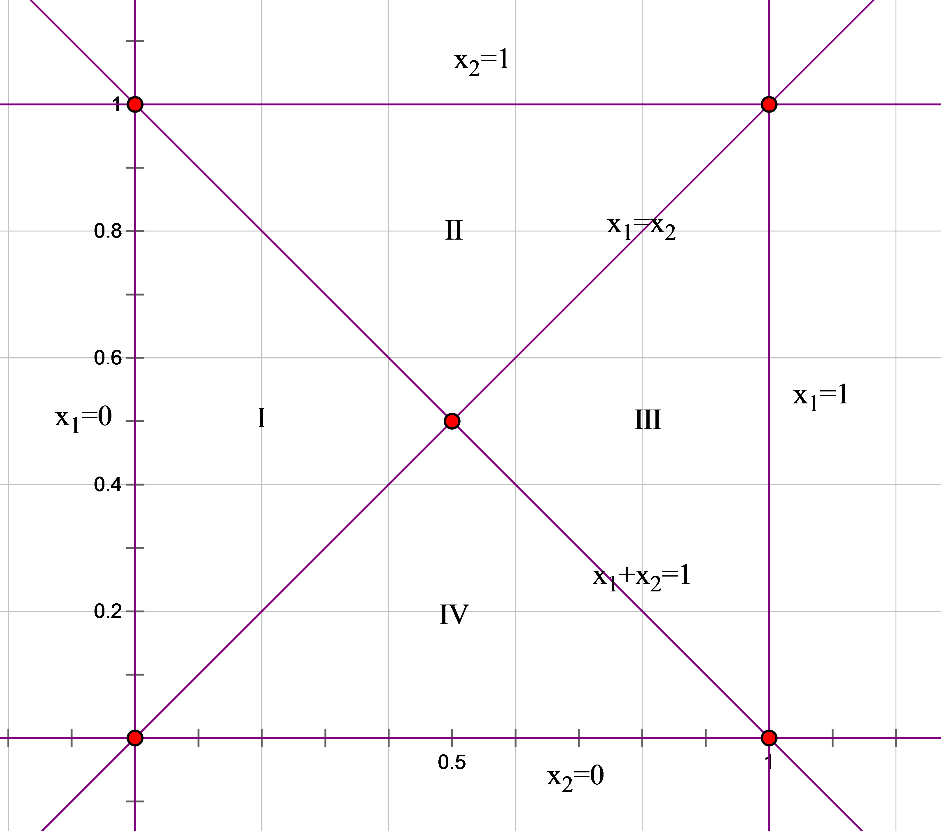
Figure 4: Solution Space of Formula 1

Figure 4 shows the linear constraints in Formula 1. The plane is splitted into 4 areas, since $b_{4}$, $b_{5}$, $b_{6}$, $b_{7}$ are always True. The pair {$b_{1}$, $b_{3}$} determines the counted areas.

• Area I: {$b_{1}$ = True, $b_{3}$ = True}. It has no lattice points.

• Area II: {$b_{1}$ = True, $b_{3}$ = False}. It has 1 lattice point: {0, 1}.

• Area III: {$b_{1}$ = False, $b_{3}$ = False}. It has 2 lattice points: {1, 0} and {1, 1}.

• Area IV: {$b_{1}$ = False, $b_{3}$ = True}. It has 1 lattice point: {0, 0}.

There are 3 Boolean solutions for Formula 1: {$b_{1}$ = True, $b_{2}$ = True, $b_{3}$ = True}, {$b_{1}$ = True, $b_{2}$ = False, $b_{3}$ = True}, and {$b_{1}$ = False, $b_{2}$ = True, $b_{3}$ = False}. Thus the volume of the solution space is $2\times vol(Area_{I})+vol(Area_{III})=0.75$. And there are $2\times 0+2=2$ integer solutions (lattice points).

Example 2

Here is an exercise for young pupils: In the following square, there are 8 sub-areas. Color them so that the neighboring sub-areas use different colors. How many different coloring schemes are there?

Obviously, this problem can be regarded as a solution counting problem. The input consists of the following inequalities:

$$xA\neq xB,~{}~{}xA\neq xD,~{}~{}xB\neq xC,~{}~{}xB\neq xD,~{}~{}xB\neq xE,$$

$$xC\neq xE,~{}~{}xD\neq xE,~{}~{}xD\neq xF,~{}~{}xD\neq xG,$$

$$xE\neq xG,~{}~{}xE\neq xH,~{}~{}xF\neq xG,~{}~{}xG\neq xH.$$

We assume that there are at most 4 colors, and execute the following command:

  % ./volce -L -w=2 examples/coloring.smt2

We find that there are 768 solutions.

Example 3

In [13], we describe a program called getop() and analyze the execution frequency of its paths. For Path1, its path condition is:

  (NOT ((c = 32) OR (c = 9) OR (c = 10))) AND
  ((c != 46) AND ((c < 48) OR (c > 57)))

Here c is a variable of type char; it can be regarded as an integer variable within the domain [-128..127].

For the above path condition, we can compute the number of solutions by executing the command:

  % ./volce -L examples/program_analysis/getopPath1.smt2

We find that the path condition has $242$ solutions. (We do not need to use the option -w=8, because the default word length is $8$.)

Given that the size of the whole search space is $256$, we conclude that the frequency of executing Path1 is about $0.945$ (i.e., $242/256$). This means, if the input string has only one character, most probably, the program will follow this path.

Another path, Path2, has the following path condition:

  ((c0 = 32) OR (c0 = 9) OR (c0 = 10)) AND
  (NOT ((c1 = 32) OR (c1 = 9) OR (c1 = 10))) AND
  (NOT ((c1 != 46) AND ((c1 < 48) OR (c1 > 57)))) AND
  (NOT ((c2 >= 48) AND (c2 <= 57))) AND
  (NOT (c2 = 46))

Given this set of constraints, and using LattE, our tool tells us that the number of solutions is 8085. The executed command is:

  % ./volce -L examples/program_analysis/getopPath2.smt2

So the path execution frequency is $8085/(256*256*256)$ which is roughly 0.00048.

Example 4

Hoare’s program FIND takes an array A[N] and an integer as input, and partitions the array into two parts.

Assume that $N=8$. We may extract two execution paths from the program, and generate the path conditions. The first path condition is the following:

  (A[0] < A[3]);  !(A[1] < A[3]);  (A[3] < A[7]);
  !(A[3] < A[6]);  !(A[2] < A[3]);  !(A[3] < A[5]);
  !(A[3] < A[4]);  (A[0] < A[4]);  (A[6] < A[4]);  (A[5] < A[4]).

Setting the word length to 4, we can find that the number of solutions is $4075920$. The executed command is:

  % ./volce -L -w=4 examples/program_analysis/FINDpath1.smt2

The second path condition is a bit more complicated:

  !(A[0] < A[3]);  (A[3] < A[7]);  (A[3] < A[6]);
  (A[3] < A[5]);  (A[3] < A[4]);  !(A[1] < A[3]);
  (A[3] < A[2]);  (A[3] < A[1]);  (A[1] < A[0]);
  (A[2] < A[0]);  !(A[0] < A[7]);  !(A[4] < A[0]);
  (A[0] < A[6]);  !(A[0] < A[5]);  (A[1] < A[7]);
  (A[2] < A[7]);  !(A[7] < A[5]);  !(A[1] < A[5]);
  !(A[2] < A[5]);  (A[5] < A[2]);  (A[2] < A[1]).

Executing the command:

  % ./volce -L -w=4 examples/program_analysis/FINDpath2.smt2

we find that the number of solutions is $87516$. So, the first path is executed much more frequently than the second one. (We assume that the input space is evenly distributed.)

Example 5

Let us try a randomly generated example (ran_5_20_8.vs). It has 5 Boolean variables, 8 numeric variable, 20 clauses and 5 linear constraints.

Execute the command:

  % ./volce -P -V -w=4 examples/ran/ran_5_20_8.vs

And we obtain the result:

Enabled PolyVest.
Enabled Vinci.
Set word length to 4.
VolCE Directory: ...
Working Directory: ...

================================

Reading Input.
Number of bool vars:     5
Number of clauses:       20
Number of numeric vars:  8
Number of linear constraints:  5

================================

Branches: 1
SATISFIABLE

================================
=========== PolyVest ===========
================================

FIRST ROUND
0Ψ8.38972e+06 * 1

SEC & LAST ROUND
0Ψ1600Ψ7.88093e+06 * 1

Total approximation: 7.88093e+06

================================

The total volume (PolyVest): 788
0930.00000000


================================
============ Vinci =============
================================

7970738.22355500 * 1

================================

The total volume (Vinci): 797073
8.22355500