From Competition to Complementarity:
Comparative Influence Diffusion and Maximization

Abstract

Influence maximization is a well-studied problem that asks for a small set of influential users from a social network, such that by targeting them as early adopters, the expected total adoption through influence cascades over the network is maximized. However, almost all prior work focuses on cascades of a single propagating entity or purely-competitive entities. In this work, we propose the Comparative Independent Cascade (Com-IC) model that covers the full spectrum of entity interactions from competition to complementarity. In Com-IC, users’ adoption decisions depend not only on edge-level information propagation, but also on a node-level automaton whose behavior is governed by a set of model parameters, enabling our model to capture not only competition, but also complementarity, to any possible degree. We study two natural optimization problems, Self Influence Maximization and Complementary Influence Maximization, in a novel setting with complementary entities. Both problems are NP-hard, and we devise efficient and effective approximation algorithms via non-trivial techniques based on reverse-reachable sets and a novel “sandwich approximation” strategy. The applicability of both techniques extends beyond our model and problems. Our experiments show that the proposed algorithms consistently outperform intuitive baselines on four real-world social networks, often by a significant margin. In addition, we learn model parameters from real user action logs.

1 Introduction

Online social networks are ubiquitous and play an essential role in our daily life. Fueled by popular applications such as viral marketing, there has been extensive research in influence and information propagation in social networks, from both theoretical and practical points of view. A key computational problem in this field is influence maximization, which asks to identify a small set of $k$ influential users (also known as seeds) from a given social network, such that by targeting them as early adopters of a new technology, product, or opinion, the expected number of total adoptions triggered by social influence cascade (or, propagation) is maximized [15, 8]. The dynamics of an influence cascade are typically governed by a stochastic diffusion model, which specifies how adoptions propagate from one user to another in the network.

Most existing work focuses on two types of diffusion models — single-entity models and pure-competition models. A single-entity model has only one propagating entity for social network users to adopt: the classic Independent Cascade (IC) and Linear Thresholds (LT) models [15] belong to this category. These models, however, ignore complex social interactions involving multiple propagating entities. Considerable work has been done to extend IC and LT models to study competitive influence maximization, but almost all models assume that the propagating entities are in pure competition and users adopt at most one of them [7, 13, 5, 21, 3, 1, 6, 16].

In reality, the relationship between different propagating entities is certainly more general than pure competition. In fact, consumer theories in economics have two well-known notions: substitute goods and complementary goods [22]. Substitute goods are similar ones that compete, and can be purchased, one in place of the other, e.g., smartphones of various brands. Complementary goods are those that tend to be purchased together, e.g,. iPhone and its accessories, computer hardware and software, etc. There are also varying degrees of substitutability and complementarity: buying a product could lessen the probability of buying the other without necessarily eliminating it; similarly, buying a product could boost the probability of buying another to any degree. Pure competition only corresponds to the special case of perfect substitute goods.

The limitation of pure-competition models can be exposed by the following example. Consider a viral marketing campaign featuring iPhone 6 and Apple Watch. It is vital to recognize the fact that Apple Watch generally needs an iPhone to be usable, and iPhone’s user experience can be greatly enhanced by a pairing Apple Watch (see, e.g., http://bit.ly/1GOqesc). Clearly none of the pure-competition models is suitable for this campaign because they do not even allow users to adopt both the phone and the watch! This motivates us to design a more powerful, expressive, yet reasonably tractable model that captures not only competition, but also complementarity, and to any possible degrees associated with these notions.

To this end, we propose the Comparative Independent Cascade model, or Com-IC for short, which, unlike most existing diffusion models, consists of two critical components that work jointly to govern the dynamics of diffusions: edge-level information propagation and a Node-Level Automaton (NLA) that ultimately makes adoption decisions based on a set of model parameters, known as the Global Adoption Probabilities (GAPs). Of these, edge-level propagation is similar to the propagation captured by the classical IC and LT models, but only controls information awareness. The NLA is a novel feature and is unique to our proposal. Indeed, the term “comparative” comes from the fact that once a user is aware, via edge-level propagation, of multiple products, intuitively she makes a comparison between them by “running” her NLA. Notice that “comparative” subsumes “competitive” and “complementary” as special cases. In theory, the Com-IC model is able to accommodate any number of propagating entities (items) and cover the entire spectrum from competition to complementarity between pairs of items, reflected by the values of GAPs.

In this work, as the first step toward comparative influence diffusion and viral marketing, we focus on the case of two items. At any time, w.r.t. any item $\mathcal{A}$, a user in the network is in one of the following four states: $\mathcal{A}$-idle, $\mathcal{A}$-suspended, $\mathcal{A}$-rejected, or $\mathcal{A}$-adopted. The NLA sets out probabilistic transition rules between states, and different GAPs are applied based on a given user’s state w.r.t. the other item $\mathcal{B}$ and the relationship between $\mathcal{A}$ and $\mathcal{B}$. Intuitively, competition (complementarity) is modeled as reduced probability (resp., increased probability) of adopting the second item after the first item is already adopted. After a user adopts an item, she propagates this information to her neighbors in the network, making them aware of the item. The neighbor may adopt the item with a certain probability, as governed by her NLA.

We then define two novel optimization problems for two complementary items $\mathcal{A}$ and $\mathcal{B}$. Our first problem, Self Influence Maximization (SelfInfMax), asks for $k$ seeds for $\mathcal{A}$ such that given a fixed set of $\mathcal{B}$-seeds, the expected number of $\mathcal{A}$-adopted nodes is maximized. The second one, Complementary Influence Maximization (CompInfMax), considers the flip side of SelfInfMax: given a fixed set of $\mathcal{A}$-seeds, find a set of $k$ seeds for $\mathcal{B}$ such that the expected increase in $\mathcal{A}$-adopted nodes thanks to $\mathcal{B}$ is maximized. To the best of our knowledge, we are the first to systematically study influence maximization for complementary items.

We show that both problems are NP-hard under Com-IC. Moreover, two important properties, submodularity and monotonicity (see §2), which would allow a greedy approximation algorithm frequently used for influence maximization, do not hold in unrestricted Com-IC model. Even when we restrict Com-IC to mutual complementarity, submodularity still does not hold in general.

To circumvent the aforementioned difficulties, we first show that submodularity holds for a subset of the complementary parameter space. We then make a non-trivial extension to the Reverse-Reachable Set (RR-set) techniques [2, 24, 23], originally proposed for influence maximization with single-entity models, to obtain effective and efficient approximation solutions to both SelfInfMax and CompInfMax. Next, we propose a novel Sandwich Approximation (SA) strategy which, for a given non-submodular set function, provides an upper bound function and/or a lower bound function, and uses them to obtain data-dependent approximation solutions w.r.t. the original function. We further note that both techniques are applicable to a larger context beyond the model and problems studied in this paper: for RR-sets, we provide a new definition and general sufficient conditions not covered by [2, 24, 23] that apply to a large family of influence diffusion models, while SA applies to the maximization of any non-submodular functions that are upper- and/or lower-bounded by submodular functions.

In experiments, we first learn GAPs from user action logs from two social networking sites – Flixster.com and Douban.com. We demonstrate that our approximation algorithms based on RR-sets and SA techniques consistently outperform several intuitive baselines, typically by a significant margin on real-world networks.

To summarize, we make the following contributions:

• We propose the Com-IC model to characterize influence diffusion dynamics of products with arbitrary degree of competition or complementarity, and identify a subset of the parameter space under which submodularity and monotonicity of influence spread hold, paving the way for approximation algorithms (§3 and §5).

• We propose two novel problems – Self Influence Maximization and Complementary Influence Maximization – for complementary products under the Com-IC model (§4).

• We show that both problems are NP-hard, and devise efficient and effective approximation solutions by non-trivial extensions to RR-set techniques and by proposing Sandwich Approximation, both having applicability beyond this work (§6).

• We conduct empirical evaluations on four real-world social networks and demonstrate the superiority of our algorithms over intuitive baselines, and also propose a methodology for learning global adoption probabilities for the Com-IC model from user action logs of social networking sites (§7).

For better readability, most of the proofs, as well as some additional theoretical and experimental results are presented in the appendix.

2 Background & Related Work

Given a graph $G=(V,E,p)$ where $p:E\to[0,1]$ specifies pairwise influence probabilities (or weights) between nodes, and $k\in\mathbb{Z}_{+}$, the influence maximization problem asks to find a set $S\subseteq V$ of $k$ seeds, activating which leads to the maximum expected number of active nodes (denoted $\sigma(S)$) [15]. Under both IC and LT models, this problem is NP-hard; Chen et al. [9, 10] showed computing $\sigma(S)$ exactly for any $S\subseteq V$ is #P-hard. Fortunately, $\sigma(\cdot)$ is a submodular and monotone function of $S$ for both IC and LT, which allows a simple greedy algorithm with an approximation factor of $1-1/e-\epsilon$, for any $\epsilon>0$ [15, 20]. A set function $f:2^{U}\to\mathbb{R}_{\geq 0}$ is submodular if for any $S\subseteq T\subseteq U$ and any $x\in U\setminus T$, $f(S\cup\{x\})-f(S)\geq f(T\cup\{x\})-T(S)$, and monotone if $f(S)\leq f(T)$ whenever $S\subseteq T\subseteq U$. Tang et al. [24, 23] proposed new randomized approximation algorithms which are orders of magnitude faster than the original greedy algorithms in [15].

In competitive influence maximization [7, 13, 5, 21, 3, 1, 6, 16] (also surveyed in [8]), a common thread is the focus on pure competition, which only allows users to adopt at most one product or opinion. Most works are from the follower’s perspective [1, 6, 13, 5], i.e., given competitor’s seeds, how to maximize one’s own spread, or minimize the competitor’s spread. Lu et al. [16] aims to maximize the total influence spread of all competitors while ensuring fair allocation.

For viral marketing with non-competing items, Datta et al. [11] studied influence maximization with items whose propagations are independent. Narayanam et al. [19] studied a setting with two sets of products, where a product can be adopted by a node only when it has already adopted a corresponding product in the other set. Their model extends LT. We depart by defining a significantly more powerful and expressive model in Com-IC, compared to theirs which only covers the special case of perfect complementarity.

Myers and Leskovec analyzed Twitter data to study the effects of different cascades on users and predicted the likelihood of a user adopting a piece of information given the cascades to which the user was previously exposed [18]. McAuley et al. used logistic regression to learn substitute/complementary relationships between products from user reviews [17]. Both studies focus on data analysis and behavior prediction and do not provide diffusion modeling for competing and complementary items, nor do they study the influence maximization problem in this context.

3 Comparative Independent Cascade Model

Review of Classical IC Model

In the IC model [15], there is just one entity (e.g., idea or product) being propagated through the network. An instance of the model has a directed graph $G=(V,E,p)$ where $p:E\to[0,1]$, and a seed set $S\subset V$. For convenience, we use $p_{u,v}$ for $p(u,v)$. At time step $0$, the seeds are active and all other nodes are inactive. Propagation proceeds in discrete time steps. At time $t$, every node $u$ that became active at $t-1$ makes one attempt to activate each of its inactive out-neighbors $v$. This can be seen as node $u$ “testing” if the edge $(u,v)$ is “live” or “blocked”. The out-neighbor $v$ becomes active at $t$ iff the edge is live. The propagation ends when no new nodes become active.

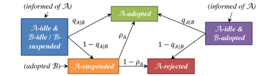
Figure 1: Com-IC model: Node-level automaton for product/item $\mathcal{A}$.

Key differences from IC model

In the Comparative IC model (Com-IC), there are at least two products. For ease of exposition, we focus on just two products $\mathcal{A}$ and $\mathcal{B}$ below. Each node can be in any of the states {idle, suspended, adopted, rejected} w.r.t. each of the products. All nodes are initially in the joint state of ($\mathcal{A}$-idle, $\mathcal{B}$-idle). One of the biggest differences between Com-IC and IC is the separation of information diffusion (edge-level) and the actual adoption decisions (node-level). Edges only control the information that flows to a node: e.g., when $u$ adopts a product, its out-neighbor $v$ may be informed of this fact. Once that happens, $v$ uses its own node level automaton (NLA) to decide which state to transit to. This depends on $v$’s current state w.r.t. the two products as well as parameters corresponding to the state transition probabilities of the NLA, namely the Global Adoption Probabilities, defined below.

A concise representation of the NLA is in Figure 1. Each state is indicated by the label. The state diagram is self-explanatory. E.g., with probability $q_{\mathcal{A}|\emptyset}$, a node transits from a state where it’s $\mathcal{A}$-idle to $\mathcal{A}$-adopted, regardless of whether it was $\mathcal{B}$-idle or $\mathcal{B}$-suspended.

From the $\mathcal{A}$-suspended state, it transits to $\mathcal{A}$-adopted w.p. $\rho_{\mathcal{A}}$ and to $\mathcal{A}$-rejected w.p. $1-\rho_{\mathcal{A}}$. The probability $\rho_{\mathcal{A}}$, called reconsideration probability, as well as the reconsideration process will be explained below. Note that in a Com-IC diffusion process defined below, not all joint state is reachable from the initial ($\mathcal{A}$-idle, $\mathcal{B}$-idle) state, e.g., ($\mathcal{A}$-idle, $\mathcal{B}$-rejected). Since all unreachable states are irrelevant to adoptions, they are negligible (details in Appendix).

Global Adoption Probability (GAP)

The Global Adoption Probabilities (GAPs), consisting of four parameters $\mathbf{Q}=(q_{\mathcal{A}|\emptyset},q_{\mathcal{A}|\mathcal{B}},q_{\mathcal{B}|\emptyset},q_{\mathcal{B}|\mathcal{A}})\in[0,1]^{4}$ are important parameters of the NLA which decide the likelihood of adoptions after a user is informed of an item. $q_{\mathcal{A}|\emptyset}$ is the probability that a user adopts $\mathcal{A}$ given that she is informed of $\mathcal{A}$ but not $\mathcal{B}$-adopted, and $q_{\mathcal{A}|\mathcal{B}}$ is the probability that a user adopts $\mathcal{A}$ given that she is already $\mathcal{B}$-adopted. A similar interpretation applies to $q_{\mathcal{B}|\emptyset}$ and $q_{\mathcal{B}|\mathcal{A}}$.

Intuitively, GAPs reflect the overall popularity of products and how they are perceived by the entire market. They are considered aggregate estimates and hence are not user specific in our model. We provide further justifications at the end of this section and describe a way to learn GAPs from user action log data in §7.

GAPs enable Com-IC to model competition and complementarity, to arbitrary degrees. We say that $\mathcal{A}$ competes with $\mathcal{B}$ iff $q_{\mathcal{B}|\mathcal{A}}\leq q_{\mathcal{B}|\emptyset}$. Similarly, $\mathcal{A}$ complements $\mathcal{B}$ iff $q_{\mathcal{B}|\mathcal{A}}\geq q_{\mathcal{B}|\emptyset}$. We include the special case of $q_{\mathcal{B}|\mathcal{A}}=q_{\mathcal{B}|\emptyset}$ in both cases above for convenience of stating our technical results, and it actually means that the propagation of $\mathcal{B}$ is completely independent of $\mathcal{A}$ (cf. Lemma 3). Competition and complementarity in the other direction are similar. The degree of competition and complementarity is determined by the difference between the two relevant GAPs, i.e., $|q_{\mathcal{B}|\mathcal{A}}-q_{\mathcal{B}|\emptyset}|$ and $|q_{\mathcal{A}|\mathcal{B}}-q_{\mathcal{A}|\emptyset}|$. For convenience, we use $\mathbf{Q}^{+}$ to refer to any set of GAPs representing mutual complementarity: $(q_{\mathcal{A}|\emptyset}\leq q_{\mathcal{A}|\mathcal{B}})\wedge(q_{\mathcal{B}|\emptyset}\leq q_{\mathcal{B}|\mathcal{A}})$, and similarly, $\mathbf{Q}^{-}$ for GAPs representing mutual competition: $(q_{\mathcal{A}|\emptyset}\geq q_{\mathcal{A}|\mathcal{B}})\wedge(q_{\mathcal{B}|\emptyset}\geq q_{\mathcal{B}|\mathcal{A}})$.

Diffusion Dynamics

Let $G=(V,E,p)$ be a directed social graph with pairwise influence probabilities. Let $S_{\mathcal{A}},S_{\mathcal{B}}\subset V$ be the seed sets for $\mathcal{A}$ and $\mathcal{B}$. Influence diffusion under Com-IC proceeds in discrete time steps. Initially, every node is $\mathcal{A}$-idle and $\mathcal{B}$-idle. At time step $0$, every $u\in S_{\mathcal{A}}$ becomes $\mathcal{A}$-adopted and every $u\in S_{\mathcal{B}}$ becomes $\mathcal{B}$-adopted. If $u\in S_{\mathcal{A}}\cap S_{\mathcal{B}}$, we randomly decide the order of $u$ adopting $\mathcal{A}$ and $\mathcal{B}$ with a fair coin. For ease of understanding, we describe the rest of the diffusion process in a modular way in Figure 2. We use $N^{+}(v)$ and $N^{-}(v)$ to denote the set of out-neighbors and in-neighbors of $v$, respectively.

We draw special attention to tie-breaking and reconsideration. Tie-breaking is used when a node’s in-neighbors adopt different products and try to inform the node at the same step. Node reconsideration concerns the situation that a node $v$ did not adopt $\mathcal{A}$ initially but later after adopting $\mathcal{B}$ it may reconsider adopting $\mathcal{A}$: when $\mathcal{B}$ competes with $\mathcal{A}$ ($q_{\mathcal{A}|\emptyset}\geq q_{\mathcal{A}|\mathcal{B}}$), $v$ will not reconsider adopting $\mathcal{A}$, but when $\mathcal{B}$ complements $\mathcal{A}$ (specifically, $q_{\mathcal{A}|\emptyset}<q_{\mathcal{A}|\mathcal{B}}$), $v$ will reconsider adopting $\mathcal{A}$. In the latter case, the probability of adopting $\mathcal{A}$, $\rho_{\mathcal{A}}$, is defined in such a way that the overall probability of adopting $\mathcal{A}$ is equal to $q_{\mathcal{A}|\mathcal{B}}$ (since $q_{\mathcal{A}|\mathcal{B}}=q_{\mathcal{A}|\emptyset}+(1-q_{\mathcal{A}|\emptyset})\rho_{\mathcal{A}}$).

Global Iteration. At every time step $t\geq 1$, for all nodes that became $\mathcal{A}$- or $\mathcal{B}$-adopted at $t-1$, their outgoing edges are tested for transition (1 below). After that, for each node $v$ that has at least one in-neighbor (with a live edge) becoming $\mathcal{A}$- and/or $\mathcal{B}$-adopted at $t-1$, $v$ is tested for possible state transition (2-4 below).

1.

Edge transition. For an untested edge $(u,v)$, flip a biased coin independently: $(u,v)$ is live w.p. $p_{u,v}$ and blocked w.p. $1-p_{u,v}$. Each edge is tested at most once in the entire diffusion process.

2.

Node tie-breaking. Consider a node $v$ to be tested at time $t$. Generate a random permutation $\pi$ of $v$’s in-neighbors (with live edges) that adopted at least one product at $t-1$. Then, test $v$ with each such in-neighbor $u$ and $u$’s adopted item ($\mathcal{A}$ and/or $\mathcal{B}$) following $\pi$. If there is a $w\in N^{-}(v)$ adopting both $\mathcal{A}$ and $\mathcal{B}$, then test both products, following their order of adoption by $w$.

3.

Node adoption. Consider the case of testing an $\mathcal{A}$-idle node $v$ for adopting $\mathcal{A}$ (Figure 1). If $v$ is not $\mathcal{B}$-adopted, then w.p. $q_{\mathcal{A}|\emptyset}$, it becomes $\mathcal{A}$-adopted and w.p. $1-q_{\mathcal{A}|\emptyset}$ it becomes $\mathcal{A}$-suspended. If $v$ is $\mathcal{B}$-adopted, then w.p. $q_{\mathcal{A}|\mathcal{B}}$, it becomes $\mathcal{A}$-adopted and w.p. $1-q_{\mathcal{A}|\mathcal{B}}$ it becomes $\mathcal{A}$-rejected. The case of adopting $\mathcal{B}$ is symmetric.

4.

Node reconsideration. Consider an $\mathcal{A}$-suspended node $v$ that just adopts $\mathcal{B}$ at time $t$. Define $\rho_{\mathcal{A}}=\max\{q_{\mathcal{A}|\mathcal{B}}-q_{\mathcal{A}|\emptyset},0\}/(1-q_{\mathcal{A}|\emptyset})$. Then, $v$ reconsiders to become $\mathcal{A}$-adopted w.p. $\rho_{\mathcal{A}}$, or $\mathcal{A}$-rejected w.p. $1-\rho_{\mathcal{A}}$. The case of reconsidering $\mathcal{B}$ is symmetric.

Figure 2: Com-IC model: diffusion dynamics

Design Considerations

The design of Com-IC not only draws on the essential elements from a classical diffusion model (IC) stemming from mathematical sociology, but also closes a gap between theory and practice, in which diffusions typically do not occur just for one product or with just one mode of pure competition. With GAPs in the NLA, the model can characterize any possible relationship between two propagating entities: competition, complementarity, and any degree associated with them. GAPs are fully capable of handling asymmetric relationship between products. E.g., an Apple Watch ($\mathcal{A}$) is complemented more by an iPhone ($\mathcal{B}$) than the other way round: many functionalities of the watch are not usable without a pairing iPhone, but an iPhone is totally functional without a watch. This asymmetric complementarity can be expressed by any GAPs satisfying $(q_{\mathcal{A}|\mathcal{B}}-q_{\mathcal{A}|\emptyset})>(q_{\mathcal{B}|\mathcal{A}}-q_{\mathcal{B}|\emptyset})\geq 0$. Furthermore, introducing NLA with GAPs and separating the propagation of product information from actual adoptions reflects Kalish’s famous characterization of new product adoption [14]: customers go through two stages – awareness followed by actual adoption. In Kalish’s theory, product awareness is propagated through word-of-mouth effects; after an individual becomes aware, she would decide whether to adopt the item based on other considerations. Edges in the network can be seen as information channels from one user to another. Once the channel is open (live), it remains so. This modeling choice is reasonable as competitive goods are typically of the same kind and complementary goods tend to be adopted together.

We remark that Com-IC encompasses previously-studied single-entity and pure-competition models as special cases. When $q_{\mathcal{A}|\emptyset}=q_{\mathcal{B}|\emptyset}=1$ and $q_{\mathcal{A}|\mathcal{B}}=q_{\mathcal{B}|\mathcal{A}}=0$, Com-IC reduces to the (purely) Competitive Independent Cascade model [8]. If, in addition, $q_{\mathcal{B}|\emptyset}$ is $0$, the model further reduces to the classic IC model.

4 Formal Problem Statements

Many interesting optimization problems can be formulated under the expressive Com-IC model. In this work, we focus on influence maximization with complementary propagating entities, since competitive viral marketing has been studied extensively (see §2). In what follows, we propose two problems. The first one, Self Influence Maximization (SelfInfMax), is a natural extension to the classical influence maximization problem [15]. The second one is the novel Complementary Influence Maximization (CompInfMax), where the objective is to maximize complementary effects (or “boost” the expected number of adoptions) by selecting the best seeds of a complementing good.

Given the seed sets $S_{\mathcal{A}},S_{\mathcal{B}}$, we first define $\sigma_{\mathcal{A}}(S_{\mathcal{A}},S_{\mathcal{B}})$ and $\sigma_{\mathcal{B}}(S_{\mathcal{A}},S_{\mathcal{B}})$ to be the expected number of $\mathcal{A}$-adopted and $\mathcal{B}$-adopted nodes, respectively under the Com-IC model. Clearly, both $\sigma_{\mathcal{A}}$ and $\sigma_{\mathcal{B}}$ are real-valued bi-set functions mapping $2^{V}\times 2^{V}$ to $[0,|V|]$, for any fixed $\mathbf{Q}$. Unless otherwise specified, GAPs are not considered as arguments to $\sigma_{\mathcal{A}}$ and $\sigma_{\mathcal{B}}$ as $\mathbf{Q}$ is constant in a given instance of Com-IC. Also, for simplicity, we may refer to $\sigma_{\mathcal{A}}(\cdot,\cdot)$ as $\mathcal{A}$-spread and $\sigma_{\mathcal{B}}(\cdot,\cdot)$ as $\mathcal{B}$-spread. The following two problems are defined in terms of $\mathcal{A}$-spread, without loss of generality.

Problem 1 (SelfInfMax).

Given a directed graph $G=(V,E,p)$ with pairwise influence probabilities, $\mathcal{B}$-seed set $S_{\mathcal{B}}\subset V$, a cardinality constraint $k$, and a set of GAPs $\mathbf{Q}^{+}$, find an $\mathcal{A}$-seed set $S_{\mathcal{A}}^{*}\subset V$ of size $k$, such that the expected number of $\mathcal{A}$-adopted nodes is maximized under Com-IC: $S_{\mathcal{A}}^{*}\in\operatorname*{arg\,max}_{T\subseteq V,|T|=k}\sigma_{\mathcal{A}}(T,S_{\mathcal{B}}).$

SelfInfMax is obviously NP-hard, as it subsumes InfMax under the classic IC model when $S_{\mathcal{B}}=\emptyset$ and $q_{\mathcal{A}|\emptyset}=q_{\mathcal{A}|\mathcal{B}}=1$. By a similar argument, it is #P-hard to compute the exact value of $\sigma_{\mathcal{A}}(S_{\mathcal{A}},S_{\mathcal{B}})$ and $\sigma_{\mathcal{B}}(S_{\mathcal{A}},S_{\mathcal{B}})$ for any given $S_{\mathcal{A}}$ and $S_{\mathcal{B}}$.

Problem 2 (CompInfMax).

Given a directed graph $G=(V,E,p)$ with pairwise influence probabilities, $\mathcal{A}$-seed set $S_{\mathcal{A}}\subset V$, a cardinality constraint $k$, and a set of GAPs $\mathbf{Q}^{+}$, find a $\mathcal{B}$-seed set $S_{\mathcal{B}}^{*}\subseteq V$ of size $k$ such that the expected increase (boost) in $\mathcal{A}$-adopted nodes is maximized under Com-IC: $S_{\mathcal{B}}^{*}\in\operatorname*{arg\,max}_{T\subseteq V,|T|=k}[\sigma_{\mathcal{A}}(S_{\mathcal{A}},T)-\sigma_{\mathcal{A}}(S_{\mathcal{A}},\emptyset)].$

Theorem 1.

CompInfMax is NP-hard.

Proof.

Let $\bf I$ be an instance of InfMax with the IC model, defined by a directed graph $G=(V,E)$ and budget $b<|V|$. We define an instance $\bf J$ of CompInfMax as follows. For each $v\in V$, create a dummy copy $v^{\prime}$ and a directed edge $(v^{\prime},v)$ with influence probability $p_{v^{\prime},v}=1$. Let $V^{\prime}$ be the set of all dummy nodes. Set $S_{\mathcal{A}}=V^{\prime}$, $q_{\mathcal{A}|\emptyset}=0$, $q_{\mathcal{A}|\mathcal{B}}=q_{\mathcal{B}|\emptyset}=q_{\mathcal{B}|\mathcal{A}}=1$. The budget $b$ of selecting $\mathcal{B}$ seeds in instance $\bf J$ is the same $b$ as in instance $\bf I$.

Claim 1.

Consider the CompInfMax instance $\bf J$. For all $\cal B$-seed sets $S_{\mathcal{B}}$, there exists a set $T_{\mathcal{B}}\subseteq V^{\prime}$ such that $\sigma_{\mathcal{A}}(S_{\mathcal{A}},T_{\mathcal{B}})\geq\sigma_{\mathcal{A}}(S_{\mathcal{A}},S_{\mathcal{B}})$.

Proof of Claim 1.

Let $v\in S_{\mathcal{B}}\cap V$ be any regular node. Assume for now that $v^{\prime}\not\in S_{\mathcal{B}}$. Let $S^{\prime}_{\mathcal{B}}$ denote the $\mathcal{B}$-seed set obtained by replacing all such $v$ by its corresponding dummy copy $v^{\prime}$. Since $S_{\mathcal{A}}=V^{\prime}$, all dummy nodes are $\mathcal{A}$-adopted and all regular nodes are $\mathcal{A}$-informed. Choosing $v^{\prime}$ to be a $\mathcal{B}$-seed makes $v^{\prime}$ and $v$ both $\mathcal{B}$-adopted, so by reconsideration $v$ becomes $\mathcal{A}$-adopted as well. Clearly, the sets of regular nodes that are $\mathcal{B}$-adopted under the configurations $(S_{\mathcal{A}},S_{\mathcal{B}})$ and $(S_{\mathcal{A}},S^{\prime}_{\mathcal{B}})$ are the same. Thus, sets of regular nodes that are $\mathcal{A}$-adopted under these configurations are also the same, which verifies the claim.

Now suppose $v,v^{\prime}\in S_{\mathcal{B}}$. We claim that there exists a dummy node outside $S_{\mathcal{B}}$, which follows from the fact that the budget $b<|V|=|V^{\prime}|$. Now, replace $v$ with any dummy node $u^{\prime}$ not in $S_{\mathcal{B}}$ and call the resulting $\mathcal{B}$-seed set $S^{\prime}_{\mathcal{B}}$. By an argument similar to the above case, we can see that every regular node that is $\mathcal{A}$-adopted under configuration $(S_{\mathcal{A}},S_{\mathcal{B}})$ is also $\mathcal{A}$-adopted under configuration $(S_{\mathcal{A}},S^{\prime}_{\mathcal{B}})$. There may be additional $\mathcal{A}$-adopted regular nodes thanks to the seed $u^{\prime}\in S^{\prime}_{\mathcal{B}}\setminus S_{\mathcal{B}}$. Again, the claim follows. Finally, if $S_{\mathcal{B}}\cap V=\emptyset$ (no regular node in $S_{\mathcal{B}}$), then the claim trivially holds as we can simply let $T_{\mathcal{B}}=S_{\mathcal{B}}$. ∎

Now consider any $T\subseteq V$ and let $\sigma_{IC}(T)$ denote the expected spread of $T$ under the IC model in $G$. Let $T^{\prime}=\{v^{\prime}\in V^{\prime}:v\in T\}$ be the set of corresponding dummy copies. Since $S_{\mathcal{A}}=V^{\prime}$, all regular nodes (in $V$) would become $\cal A$-informed when $S_{\mathcal{B}}=\emptyset$. Now set $S_{\mathcal{B}}=T^{\prime}$, which would make all nodes in $T$ (regular) become $\mathcal{B}$-adopted, and then $\mathcal{A}$-adopted (by reconsideration), and further propagate both $\mathcal{A}$ and $\mathcal{B}$ over the network. Hence,

$$\sigma_{IC}(T)=\sigma_{\mathcal{A}}(S_{\mathcal{A}},T^{\prime})-n,$$ (1)

where $n=_{\mathrm{def}}|V|=|V^{\prime}|$.

Next, to prove the theorem, it suffices to show:

Claim 2.

The subset $T_{*}\subset V$ is an optimal solution to the InfMax (with IC model) instance ${\bf I}$ if and only if $T_{*}^{\prime}\subset V^{\prime}$ is an optimal solution to the CompInfMax instance $\bf J$ under the Com-IC model, where $T_{*}^{\prime}=\{v^{\prime}\in V^{\prime}:v\in T_{*}\}$.

Proof of Claim 2.

$(\Longrightarrow)$: Suppose for a contradiction that $T_{*}^{\prime}$ is suboptimal to $\bf J$. Let $X^{\prime}$ be an optimal solution to $\bf J$ instead, which implies that $\sigma_{\mathcal{A}}(S_{\mathcal{A}},X^{\prime})>\sigma_{\mathcal{A}}(S_{\mathcal{A}},T_{*}^{\prime})$.

If $X^{\prime}$ contains only dummy copies, let $X$ be the corresponding set of regular nodes. Then, by Eq. (1),

$$\sigma_{\mathcal{A}}(S_{\mathcal{A}},X^{\prime})=\sigma_{IC}(X)+n>\sigma_{\mathcal{A}}(S_{\mathcal{A}},T_{*}^{\prime})=\sigma_{IC}(T_{*})+n.$$

Hence $\sigma_{IC}(X)>\sigma_{IC}(T_{*})$, contradicting to the fact that $T_{*}$ is optimal to ${\bf I}$.

If $X^{\prime}$ contains at least one regular node, then by repeated application of Claim 1, we can obtain a $\mathcal{B}$-seed set with no regular nodes and furthermore dominates $X^{\prime}$ w.r.t. $\mathcal{A}$-spread. Thus, w.l.o.g. we can ignore $\mathcal{B}$-seed sets containing regular nodes.

$(\Longleftarrow)$: Let $T_{*}^{\prime}$ be an optimal solution to $\bf J$. By the same domination argument, we can assume w.l.o.g. that $T_{*}^{\prime}$ consists of only dummy nodes. Then, the optimality of $T_{*}$ for instance $\bf I$ can be argued using Eq. (1) in an identical manner to the above. ∎

This completes the proof that CompInfMax is NP-hard. ∎

From the formulation of CompInfMax, we can intuitively see that the placement of $\mathcal{B}$-seeds will be heavily dependent on the existing $\mathcal{A}$-seeds. For example, if $S_{\mathcal{A}}$ and $S_{\mathcal{B}}$ are in two different connected components of the graph, then evidently the boost is zero. In contrast, if they are rather close and can influence roughly the same region in the graph, the boost is likely to be high. Indeed, for the special case where $q_{\mathcal{B}|\emptyset}=1$ and $k\geq|S_{\mathcal{A}}|$, directly “copying” $\mathcal{A}$-seeds to be $\mathcal{B}$-seeds will give the optimal boost. However, this in no way diminishes the value of this problem, as Theorem 1 shows the NP-hardness in the general case.

Theorem 2.

For CompInfMax, when $q_{\mathcal{B}|\emptyset}=1$ and $k\geq|S_{\mathcal{A}}|$, we can solve the problem optimally by setting $S_{\mathcal{B}}^{*}$ to be $S_{\mathcal{A}}\cup X$, where $X$ is an arbitrary set in $V\setminus S_{\mathcal{A}}$ with size $k-|S_{\mathcal{A}}|$, that is $\sigma_{\mathcal{A}}(S_{\mathcal{A}},S_{\mathcal{A}}\cup X)=\max_{T\subseteq V,|T|=k}\sigma_{\mathcal{A}}(S_{\mathcal{A}},T)$.

The proof of this theorem relies on the possible world model, which is defined in the next section. Hence, we defer to the proof to the appendix.

5 Properties of Com-IC

Since neither of SelfInfMax and CompInfMax can be solved in PTIME unless P = NP, we explore approximation algorithms by studying submodularity and monotonity for Com-IC, which may pave the way for designing approximation algorithms. Note that $\sigma_{\mathcal{A}}$ is a bi-set function taking arguments $S_{\mathcal{A}}$ and $S_{\mathcal{B}}$, so we analyze the properties w.r.t. each of the two arguments. As appropriate, we refer to the properties of $\sigma_{\mathcal{A}}$ w.r.t. $S_{\mathcal{A}}$ ($S_{\mathcal{B}}$) as self-monotonicity (resp., cross-monotonicity) and self-submodularity (resp., cross-submodularity).

5.1 An Equivalent Possible World Model

To facilitate a better understanding of Com-IC and our analysis on submodularity, we define a Possible World (PW) model that provides an equivalent view of the Com-IC model. Given a graph $G=(V,E,p)$ and a diffusion model, a possible world consists of a deterministic graph sampled from a probability distribution over all subgraphs of $G$. For Com-IC, we also need some variables for each node to fix the outcomes of random events in relation to the NLA (adoption, tie-breaking, and reconsideration), so that influence cascade is fully deterministic in a single possible world.

Generative Rules. Retain each edge $(u,v)\in E$ w.p. $p_{u,v}$ (live edge) and drop it w.p. $1-p_{u,v}$ (blocked edge). This generates a possible world $W$ with $G_{W}=(V,E_{W})$, $E_{W}$ being the set of live edges. Next, for every node $v\in V$, we

1. choose “thresholds” $\alpha_{\mathcal{A}}^{v,W}$ and $\alpha_{\mathcal{B}}^{v,W}$ independently and uniformly at random from $[0,1]$, for comparison with GAPs in adoption decisions (when $W$ is clear from context, we write $\alpha_{\mathcal{A}}^{v}$ and $\alpha_{\mathcal{B}}^{v}$);

2. generate a random permutation $\pi_{v}^{W}$ of all in-neighbors $u\in N^{-}(v)$ (for tie-breaking);

3. sample a discrete value $\tau_{v}^{W}\in\{\mathcal{A},\mathcal{B}\}$, where each value has a probability of $0.5$ (used for tie-breaking in case $v$ is a seed of both $\mathcal{A}$ and $\mathcal{B}$).

Deterministic cascade in a PW. At time step $0$, nodes in $S_{\mathcal{A}}$ and $S_{\mathcal{B}}$ first become $\mathcal{A}$-adopted and $\mathcal{B}$-adopted, respectively (ties, if any, are broken based on $\tau_{v}$). Then, iteratively for each step $t\geq 1$, a node $v$ becomes “reachable” by $\mathcal{A}$ at time step $t$ if $t$ is the length of a shortest path from any seed $u\in S_{\mathcal{A}}$ to $v$ consisting entirely of live edges and $\mathcal{A}$-adopted nodes. Node $v$ then becomes $\mathcal{A}$-adopted at step $t$ if $\alpha_{\mathcal{A}}^{v}\leq x$, where $x=q_{\mathcal{A}|\emptyset}$ if $v$ is not $\mathcal{B}$-adopted, otherwise $x=q_{\mathcal{A}|\mathcal{B}}$. For re-consideration, suppose $v$ just becomes $\mathcal{B}$-adopted at step $t$, while being $\mathcal{A}$-suspended (i.e., $v$ was reachable by $\mathcal{A}$ before $t$ steps but $\alpha_{\mathcal{A}}^{v}>q_{\mathcal{A}|\emptyset}$). Then, $v$ adopts $\mathcal{A}$ if $\alpha_{\mathcal{A}}^{v}\leq q_{\mathcal{A}|\mathcal{B}}$. The reachability and reconsideration tests of $\mathcal{B}$ are symmetric. For tie-breaking, if $v$ is reached by both $\mathcal{A}$ and $\mathcal{B}$ at $t$, the permutation $\pi_{v}$ is used to determine the order in which $\mathcal{A}$ and $\mathcal{B}$ are considered. In addition, if $v$ is reached by $\mathcal{A}$ and $\mathcal{B}$ from the same in-neighbor, e.g., $u$, then the informing order follows the order in which $u$ adopts $\mathcal{A}$ and $\mathcal{B}$.

The following lemma establishes the equivalence between this possible world model and Com-IC. This allows us to analyze monotonicity and submodularity using the PW model only.

Lemma 1.

For any fixed $\mathcal{A}$-seed set $S_{\mathcal{A}}$ and $\mathcal{B}$-seed set $S_{\mathcal{B}}$, the joint distributions of the sets of $\mathcal{A}$-adopted nodes and $\mathcal{B}$-adopted nodes obtained $(i)$ by running a Com-IC diffusion from $S_{\mathcal{A}}$ and $S_{\mathcal{B}}$ and $(ii)$ by randomly sampling a possible world $W$ and running a deterministic cascade from $S_{\mathcal{A}}$ and $S_{\mathcal{B}}$ in $W$, are the same.

Equivalence Classes of Possible Worlds. Notice that in a possible world, $\alpha_{\mathcal{A}}^{v}$ and $\alpha_{\mathcal{B}}^{v}$ are both real values in the interval $[0,1]$. Thus in theory, the total number of possible worlds is infinite. In what follows, we establish a finite number of equivalence classes of possible worlds. This facilitates theoretical analysis of the model, e.g., the proof of Theorem 2 makes use of this property (see appendix).

From the perspective of influence propagation dynamics under Com-IC, especially the final states of each node w.r.t. both products, the exact values of $\alpha_{\mathcal{A}}^{v}$ and $\alpha_{\mathcal{B}}^{v}$ do not matter. Instead, we only need to know the ranges that $\alpha_{\mathcal{A}}^{v}$ and $\alpha_{\mathcal{B}}^{v}$ fall in. For $\alpha_{\mathcal{A}}^{v}$, the ranges are

• $[0,q_{\mathcal{A}|\emptyset})$, $[q_{\mathcal{A}|\emptyset},q_{\mathcal{A}|\mathcal{B}})$, $[q_{\mathcal{A}|\mathcal{B}},1]$ when $q_{\mathcal{A}|\emptyset}\leq q_{\mathcal{A}|\mathcal{B}}$,

• $[0,q_{\mathcal{A}|\mathcal{B}})$, $[q_{\mathcal{A}|\mathcal{B}},q_{\mathcal{A}|\emptyset})$, $[q_{\mathcal{A}|\emptyset},1]$ when $q_{\mathcal{A}|\mathcal{B}}<q_{\mathcal{A}|\emptyset}$.

Likewise for $\alpha_{\mathcal{B}}^{v}$, they are:

• $[0,q_{\mathcal{B}|\emptyset})$, $[q_{\mathcal{B}|\emptyset},q_{\mathcal{B}|\mathcal{A}})$, $[q_{\mathcal{B}|\mathcal{A}},1]$ when $q_{\mathcal{B}|\emptyset}\leq q_{\mathcal{B}|\mathcal{A}}$,

• $[0,q_{\mathcal{B}|\mathcal{A}})$, $[q_{\mathcal{B}|\mathcal{A}},q_{\mathcal{B}|\emptyset})$, $[q_{\mathcal{B}|\emptyset},1]$ when $q_{\mathcal{B}|\mathcal{A}}<q_{\mathcal{B}|\emptyset}$.

Given two possible worlds $W_{1}$ and $W_{2}$, we say that are equivalent iff each node $v\in V$ satisfies all of the following conditions:

1. $\alpha_{\mathcal{A}}^{v,W_{1}}$ and $\alpha_{\mathcal{A}}^{v,W_{2}}$ fall into the same range;

2. $\alpha_{\mathcal{B}}^{v,W_{1}}$ and $\alpha_{\mathcal{B}}^{v,W_{2}}$ also fall into the same range;

3. $\pi_{v}^{W_{1}}=\pi_{v}^{W_{2}}$ (same order of in-neighbours in both worlds);

4. $\tau_{v}^{W_{1}}=\tau_{v}^{W_{2}}$.

Clearly, for any two possible worlds $W_{1}$ and $W_{2}$ in the same equivalence class, by model definition we have

$$\sigma_{\mathcal{A}}^{W_{1}}(S_{\mathcal{A}},S_{\mathcal{B}})=\sigma_{\mathcal{A}}^{W_{2}}(S_{\mathcal{A}},S_{\mathcal{B}}),\text{ and }\sigma_{\mathcal{B}}^{W_{1}}(S_{\mathcal{A}},S_{\mathcal{B}})=\sigma_{\mathcal{B}}^{W_{2}}(S_{\mathcal{A}},S_{\mathcal{B}}).$$

for any $\mathcal{A}$-seed set $S_{\mathcal{A}}$ and $\mathcal{B}$-seed set $S_{\mathcal{B}}$.

In view of the above, for any equivalence class ${\bf W}$ of possible worlds, by $\sigma_{\mathcal{A}}^{{\bf W}}(S_{\mathcal{A}},S_{\mathcal{B}})$, without any ambiguity we mean $\sigma_{\mathcal{A}}^{W}(S_{\mathcal{A}},S_{\mathcal{B}})$, where $W\in{\bf W}$ is any possible world in the equivalence class ${\bf W}$. It is straightforward to verify that the total number of equivalence classes is finite, as opposed to the total number of possible worlds, which is uncountable.

Let $\Pr[{\bf W}]$ denote the total probability mass of all the possible worlds that belong to $\bf W$. In principle, this probability can be computed using integration over $\alpha_{\mathcal{A}}^{v}$’s and $\alpha_{\mathcal{B}}^{v}$’s, as there are still an uncountable number of possible worlds in any given equivalence class. An alternative method that does not involve integration is to look at the ranges in which $\alpha_{\mathcal{A}}^{v}$’s and $\alpha_{\mathcal{B}}^{v}$’s fall. For example, $\Pr[q_{\mathcal{A}|\emptyset}\leq\alpha_{\mathcal{A}}^{v}<q_{\mathcal{A}|\mathcal{B}}]=q_{\mathcal{A}|\mathcal{B}}-q_{\mathcal{A}|\emptyset}$ (assuming complementarity). This is correct as the $\alpha$-values are sampled uniformly at random from the interval $[0,1]$. We can then express the expected spread function using a linear combination of all equivalence classes:

$$\sigma_{\mathcal{A}}(S_{\mathcal{A}},S_{\mathcal{B}})=\sum_{\bf W}\Pr[{\bf W}]\cdot\sigma_{\mathcal{A}}^{\bf W}(S_{\mathcal{A}},S_{\mathcal{B}}),$$ (2)

where $\sigma_{\mathcal{A}}^{\bf W}(S_{\mathcal{A}},S_{\mathcal{B}})$ can be computed deterministically as we mentioned earlier in this subsection.

5.2 Monotonicity

It turns out that when $\mathcal{A}$ competes with $\mathcal{B}$ while $\mathcal{B}$ complements $A$, monotonicity does not hold in general (see Appendix for counter-examples). But note that these cases are rather unnatural. Hence, we focus on mutual competition ($\mathbf{Q}^{-}$) and mutural complementary cases ($\mathbf{Q}^{+}$), for which we can show self- and cross-monotonicity do hold.

Theorem 3.

For any fixed $\mathcal{B}$-seed set $S_{\mathcal{B}}$, $\sigma_{\mathcal{A}}(S_{\mathcal{A}},S_{\mathcal{B}})$ is monotonically increasing in $S_{\mathcal{A}}$ for any set of GAPs in $\mathbf{Q}^{+}$ and $\mathbf{Q}^{-}$. Also, $\sigma_{\mathcal{A}}(S_{\mathcal{A}},S_{\mathcal{B}})$ is monotonically increasing in $S_{\mathcal{B}}$ for any GAPs in $\mathbf{Q}^{+}$, and monotonically decreasing in $S_{\mathcal{B}}$ for any $\mathbf{Q}^{-}$.

5.3 Submodularity in Complementary Setting

Next, we analyze self-submodularity and cross-submodularity for mutual complementary cases ($\mathbf{Q}^{+}$) that has direct impact on SelfInfMax and CompInfMax. The analysis for $\mathbf{Q}^{-}$ is deferred to the appendix.

For self-submodularity, we show that it is satisfied in the case of “one-way complementarity”, i.e., $\mathcal{B}$ complements $\mathcal{A}$ ($q_{\mathcal{A}|\emptyset}\leq q_{\mathcal{A}|\mathcal{B}}$), but $\mathcal{A}$ does not affect $\mathcal{B}$ ($q_{\mathcal{B}|\emptyset}=q_{\mathcal{B}|\mathcal{A}}$), or vise versa (Theorem 4). We will also show the $\sigma_{\mathcal{A}}$ is cross-submodular in $S_{\mathcal{B}}$ when $q_{\mathcal{B}|\mathcal{A}}=1$ (Theorem 5). However, both properties are not satisfied in general (see appendix for counter-examples). We give two useful lemmas first, and thanks to Lemma 2 below, we may assume w.l.o.g. that tie-breaking always favors $\mathcal{A}$ in complementary cases.

Lemma 2.

Consider any Com-IC instance with $\mathbf{Q}^{+}$. Given fixed $\mathcal{A}$- and $\mathcal{B}$-seed sets, for all nodes $v\in V$, all permutations of $v$’s in-neighbors are equivalent in determining if $v$ becomes $\mathcal{A}$-adopted and $\mathcal{B}$-adopted, and thus the tie-breaking rule is not needed for mutual complementary case.

Lemma 3.

In the Com-IC model, if $\mathcal{B}$ is indifferent to $\mathcal{A}$ (i.e., $q_{\mathcal{B}|\mathcal{A}}=q_{\mathcal{B}|\emptyset}$), then for any fixed $\mathcal{B}$ seed set $S_{\mathcal{B}}$, the probability distribution over sets of $\mathcal{B}$-adopted nodes is independent of $\mathcal{A}$-seed set. Symmetrically, the probability distribution over sets of $\mathcal{A}$-adopted nodes is also independent of $\mathcal{B}$-seed set if $\mathcal{A}$ is indifferent to $\mathcal{B}$.

Theorem 4.

For any instance of Com-IC model with $q_{\mathcal{A}|\emptyset}\leq q_{\mathcal{A}|\mathcal{B}}$ and $q_{\mathcal{B}|\emptyset}=q_{\mathcal{B}|\mathcal{A}}$, $(i)$. $\sigma_{\mathcal{A}}$ is self-submodular w.r.t. $\mathcal{A}$ seed set $S_{\mathcal{A}}$, for any fixed $\mathcal{B}$-seed set $S_{\mathcal{B}}$. $(ii)$. $\sigma_{\mathcal{B}}$ is self-submodular w.r.t. $\mathcal{B}$ seed set $S_{\mathcal{B}}$ and is independent of $\mathcal{A}$-seed set $S_{\mathcal{A}}$.

Proof.

First, $(ii)$ holds trivially. By Lemma 3, $\mathcal{A}$ does not affect $\mathcal{B}$’s diffusion in any sense. Thus, $\sigma_{\mathcal{B}}(S_{\mathcal{A}},S_{\mathcal{B}})=\sigma_{\mathcal{B}}(\emptyset,S_{\mathcal{B}})$. It can be shown that the function $\sigma_{\mathcal{B}}(\emptyset,S_{\mathcal{B}})$ is both monotone and submodular w.r.t. $S_{\mathcal{B}}$, for any $q_{\mathcal{B}|\emptyset}$, through a straightforward extension to the proof of Theorem 2.2 in Kempe et al. [15].

For $(i)$, first we fix a possible world $W$ and a $\mathcal{B}$-seed set $S_{\mathcal{B}}$. Let $\Phi_{\mathcal{A}}^{W}(S_{\mathcal{A}})$ be the set of $\mathcal{A}$-adopted nodes in possible world $W$ with $\mathcal{A}$-seed set $S_{\mathcal{A}}$ ($S_{\mathcal{B}}$ omitted when it is clear from the context). Consider two sets $S\subseteq T\subseteq V$, some node $u\in V\setminus T$, and finally a node $v\in\Phi_{\mathcal{A}}^{W}(T\cup\{u\})\setminus\Phi_{\mathcal{A}}^{W}(T)$. There must exist a live-edge path $P_{\mathcal{A}}$ from $T\cup\{u\}$ consisting entirely of $\mathcal{A}$-adopted nodes. We denote by $w_{0}\in T\cup\{u\}$ the origin of $P_{\mathcal{A}}$.

We first prove a key claim: $P_{\mathcal{A}}$ remains $\mathcal{A}$-adopted when $S_{\mathcal{A}}=\{w_{0}\}$. Consider any node $w_{i}\in P_{\mathcal{A}}$. In this possible world, if $\alpha_{\mathcal{A}}^{w_{i}}\leq q_{\mathcal{A}|\emptyset}$, then regardless of the diffusion of $\mathcal{B}$, $w_{i}$ will adopt $\mathcal{A}$ as long as its predecessor $w_{i-1}$ adopts $\mathcal{A}$. If $q_{\mathcal{A}|\emptyset}<\alpha_{\mathcal{A}}^{w_{i}}\leq q_{\mathcal{A}|\mathcal{B}}$, then there must also be a live-edge path $P_{\mathcal{B}}$ from $S_{\mathcal{B}}$ to $w_{i}$ that consists entirely of $\mathcal{B}$-adopted nodes, and it boosts $w_{i}$ to adopt $\mathcal{A}$. Since $q_{\mathcal{B}|\emptyset}=q_{\mathcal{B}|\mathcal{A}}$, $\mathcal{A}$ has no effect on $\mathcal{B}$-propagation (Lemma 3), and $P_{\mathcal{B}}$ always exists and all nodes on $P_{\mathcal{B}}$ would still be $\mathcal{B}$-adopted through $S_{\mathcal{B}}$ (fixed) irrespective of $\mathcal{A}$-seeds. Thus, $P_{\mathcal{B}}$ always boosts $w_{i}$ to adopt $\mathcal{A}$ as long as $w_{i-1}$ is $\mathcal{A}$-adopted. Hence, the claim holds by a simple induction on $P_{\mathcal{A}}$ starting from $w_{0}$.

Then, it is easy to see $w_{0}$ = $u$. Suppose otherwise, then $w_{0}\in T$ must be true. By the claim above and self-monotonicity of $\sigma_{\mathcal{A}}$ (Theorem 3), $v\in\Phi_{\mathcal{A}}^{W}(\{w_{0}\})$ implies $w\in\Phi_{\mathcal{A}}^{W}(T)$, a contradiction. Therefore, we have $v\not\in\Phi_{\mathcal{A}}^{W}(S)$ and $v\in\Phi_{\mathcal{A}}^{W}(S\cup\{u\})$. This by definition implies $|\Phi_{\mathcal{A}}^{W}(\cdot)|$ is submodular for any $W$ and $S_{\mathcal{B}}$, which is sufficient to show that $\sigma_{\mathcal{A}}(S_{\mathcal{A}},S_{\mathcal{B}})$ is submodular in $S_{\mathcal{A}}$. ∎

Theorem 5.

In any instance of Com-IC with mutual complementarity $\mathbf{Q}^{+}$, $\sigma_{\mathcal{A}}$ is cross-submodular w.r.t. $\mathcal{B}$-seed set $S_{\mathcal{B}}$, for any fixed $A$-seed set, as long as $q_{\mathcal{B}|\mathcal{A}}=1$.

Proof.

We first fix an $\mathcal{A}$-seed set $S_{\mathcal{A}}$. Consider any possible world $W$. Let $\Psi^{W}_{\mathcal{A}}(S_{\mathcal{B}})$ be the set of $\mathcal{A}$-adopted nodes in $W$ with $\mathcal{B}$ seed-set $S_{\mathcal{B}}$ (and $\mathcal{A}$-seed set $S_{\mathcal{A}}$). Consider $\mathcal{B}$-seed sets $S\subseteq T\subseteq V$ and another $\mathcal{B}$-seed $u\in V\setminus T$. It suffices to show that for any $v\in\Psi^{W}_{\mathcal{A}}(T\cup\{u\})\setminus\Psi^{W}_{\mathcal{A}}(T)$, we have $v\in\Psi^{W}_{\mathcal{A}}(S\cup\{u\})\setminus\Psi^{W}_{\mathcal{A}}(S)$.

Let an $\mathcal{A}$-path be a live-edge path from some $\mathcal{A}$-seed such that all nodes on the path adopt $\mathcal{A}$, and $\mathcal{B}$-path is defined symmetrically. If a node $w$ has $\alpha_{\mathcal{A}}^{w}\leq q_{\mathcal{A}|\emptyset}$, we say that $w$ is $\mathcal{A}$-ready, meaning that $w$ is ready for $\mathcal{A}$ and will adopt $\mathcal{A}$ if it is informed of $\mathcal{A}$, regardless of its status on $\mathcal{B}$. We say a path from $S_{\mathcal{A}}$ is an $\mathcal{A}$-ready path if all nodes on the path (except the starting $\mathcal{A}$-seed) are $\mathcal{A}$-ready. It is clear that all nodes on an $\mathcal{A}$-ready path would always adopt $\mathcal{A}$ regardless of $\mathcal{B}$-seeds. We define $\mathcal{B}$-ready nodes and paths symmetrically. We can show the following claim.

Claim 3.

On any $\mathcal{A}$-path $P_{\mathcal{A}}$, if some node $w$ adopts $\mathcal{B}$ and all nodes before $w$ on $P_{\mathcal{A}}$ are $\mathcal{A}$-ready, then every node following $w$ on $P_{\mathcal{A}}$ adopts both $\mathcal{A}$ and $\mathcal{B}$, regardless of the actual $\mathcal{B}$-seed set.

Now consider the case of $S_{\mathcal{B}}=T\cup\{u\}$ first. Since $v\in\Psi^{W}_{\mathcal{A}}(T\cup\{u\})$, there must be an $\mathcal{A}$-path $P_{\mathcal{A}}$ from some node $w_{0}\in S_{\mathcal{A}}$ to $v$. If path $P_{\mathcal{A}}$ is $\mathcal{A}$-ready, then regardless of $\mathcal{B}$ seeds, all nodes on $P_{\mathcal{A}}$ would always be $\mathcal{A}$-adopted, but this contradicts the assumption that $v\not\in\Psi^{W}_{\mathcal{A}}(T)$. Therefore, there exists some node $w$ that is not $\mathcal{A}$-ready, i.e., $q_{\mathcal{A}|\emptyset}<\alpha^{w}_{\mathcal{A}}\leq q_{\mathcal{A}|\mathcal{B}}$. Let $w$ be the first non-$\mathcal{A}$-ready node on path $P_{\mathcal{A}}$. Then $w$ must have adopted $\mathcal{B}$ to help it adopt $\mathcal{A}$, and $\alpha^{w}_{\mathcal{B}}\leq q_{\mathcal{B}|\emptyset}$. We can show the following key claim.

Claim 4.

There is a $\mathcal{B}$-path $P_{\mathcal{B}}$ from some $\mathcal{B}$-seed $x_{0}\in T\cup\{u\}$ to $w$, such that even if $x_{0}$ is the only $\mathcal{B}$-seed, $w$ still adopts $\mathcal{B}$.

With the key Claim 4, the rest of the proof follows the standard argument as in the other proofs. In particular, since even when $x_{0}$ is the only $\mathcal{B}$-seed, $w$ can still be $\mathcal{B}$-adopted, then by Claim 3, $v$ would be $\mathcal{A}$-adopted in this case. Thus we know that $x_{0}$ must be $u$, because otherwise it contradicts our assumption that $v\not\in\Psi^{W}_{\mathcal{A}}(T)$ (also relying on the cross-monotonicity proof made for Theorem 3). Then again by the cross-monotonicity, we know that $v\in\Psi^{W}_{\mathcal{A}}(S\cup\{u\})$, but $v\not\in\Psi^{W}_{\mathcal{A}}(S)$. This completes our proof. ∎

6 Approximation Algorithms

We first review the state-of-the-art in influence maximization and then derive a general framework (§6.1) to obtain approximation algorithms for SelfInfMax (§6.2) and CompInfMax (§6.3).

TIM algorithm. For influence maximization, Tang et al. [24] proposed the Two-phase Influence Maximization (TIM) algorithm that produces a $(1-1/e-\epsilon)$-approximation with at least $1-|V|^{-\ell}$ probability in $O((k+\ell)(|E|+|V|)\log|V|/\epsilon^{2})$ expected running time. It is based on the concept of Reverse-Reachable sets (RR-sets) [2], and applies to the Triggering model [15] that generalizes both IC and LT. TIM is orders of magnitude faster than greedy algorithm with Monte Carlo simulations [15], while still giving approximation solutions with high probability. Recently they propose a new improvement [23], which significantly reduces the number of RR-sets generated using martingale analysis. To tackle SelfInfMax and CompInfMax, we primarily focus on the challenging task of correctly generating RR-sets in Com-IC and other more general models, which is orthogonal to the contributions of [23]. Hereafter we focus on the framework of [24]. Due to the much more complex dynamics involved in Com-IC, adapting TIM to solve SelfInfMax and CompInfMax is far from trivial, as we shall show.

Reverse-Reachable Sets. In a deterministic (directed) graph $G^{\prime}=(V^{\prime},E^{\prime})$, for a fixed $v\in V^{\prime}$, all nodes that can reach $v$ form an RR-set rooted at $v$ [2], denoted $R(v)$. A random RR set encapsulates two levels of randomness: ($i$) a “root” node $v$ is randomly chosen from the graph, and ($ii$) a deterministic graph is sampled according to a certain probabilistic rule that retains a subset of edges from the graph. E.g., for the IC model, each edge $(u,v)\in E$ is removed w.p. $(1-p_{u,v})$, independently. TIM first computes a lower bound on the optimal solution value and uses this bound to derive the number of random RR-sets to be sampled, denoted $\theta$. To guarantee approximation solutions, $\theta$ must satisfy:

$$\theta\geq\epsilon^{-2}(8+2\epsilon)|V|\cdot\frac{\ell\log|V|+\log\binom{|V|}{k}+\log 2}{\mathit{OPT}_{k}},$$ (3)

where $\mathit{OPT}_{k}$ is the optimal influence spread achievable amongst all size-$k$ sets, and $\epsilon$ represents the trade-off between efficiency and quality: a smaller $\epsilon$ implies more RR-sets (longer running time), but gives a better approximation factor. The approximation guarantee of TIM relies on a key result from [2], re-stated here:

Proposition 1 (Lemma 9 in [24]).

Fix a set $S\subseteq V$ and a node $v\in V$. Under the Triggering model, let $\rho_{1}$ be the probability that $S$ activates $v$ in a cascade, and $\rho_{2}$ be the probability that $S$ overlaps with a random RR-set $R(v)$ rooted at $v$. Then, $\rho_{1}=\rho_{2}$.

6.1 A General Solution Framework

We use Possible World (PW) models to generalize the theory in [2, 24]. For a generic stochastic diffusion model $M$, an equivalent PW model $M^{\prime}$ is a model that specifies a distribution over $\mathcal{W}$, the set of all possible worlds, where influence diffusion in each possible world in $\cal W$ is deterministic. Further, given a seed set (or two seed sets $S_{\mathcal{A}}$ and $S_{\mathcal{B}}$ as in Com-IC), the distribution of the sets of active nodes (or $\mathcal{A}$- and $\mathcal{B}$-adopted nodes in Com-IC) in $M$ is the same as the corresponding distribution in $M^{\prime}$. Then, we define a generalized concept of RR-set through the PW model:

Definition 1 (General RR-Set).

For each possible world $W\in\mathcal{W}$ and a given node $v$ (a.k.a. root), the reverse reachable set (RR-set) of $v$ in $W$, denoted by $R_{W}(v)$, consists of all nodes $u$ such that the singleton set $\{u\}$ would activate $v$ in $W$. A random RR-set of $v$ is a set $R_{W}(v)$ where $W$ is randomly sampled from $\mathcal{W}$ using the probability distribution given in $M^{\prime}$.

It is easy to see that Definition 1 encompasses the RR-set definition in [2, 24] for IC, LT, and Triggering models as special cases. For the entire solution framework to work, the key property that RR-sets need to satisfy is the following:

Definition 2 (Activation Equivalence Property).

Let $M$ be a stochastic diffusion model and $M^{\prime}$ be its equivalent possible world model. Let $G=(V,E,p)$ be a graph. Then, RR-sets have the Activation Equivalence Property if for any fixed $S\subseteq V$ and any fixed $v\in V$, the probability that $S$ activates $v$ according to $M$ is the same as the probability that $S$ overlaps with a random RR-set generated from $v$ in a possible world in $M^{\prime}$.

As shown in [24], the entire correctness and complexity analysis is based on the above property, and in fact in their latest improvement [23], they directly use this property as the definiton of general RR-sets. Proposition 1 shows that the activation equivalence property holds for the triggering model. We now provide a more general sufficient condition for the activation equivalence property to hold (Lemma 5), which gives concrete conditions on when the RR-set based framework would work. More specifically, we show that for any diffusion model $M$, if there is an equivalent PW model $M^{\prime}$ of which all possible worlds satisfy the following two properties, then RR-sets have the activation equivalence property.

Possible World Properties

• (P1): Given two seed sets $S\subseteq T$, if a node $v$ can be activated by $S$ in a possible world $W$, then $v$ shall also be activated by $T$ in $W$.

• (P2): If a node $v$ can be activated by $S$ in a possible world $W$, then there exists $u\in S$ such that the singleton seed set $\{u\}$ can also activate $v$ in $W$. In fact, (P1) and (P2) are equivalent to monotonicity and submodularity, as we formally state below.

Lemma 4.

Let $W$ be a fixed possible world. Let $f_{v,W}(S)$ be an indicator function that takes on $1$ if $S$ can activate $v$ in $W$, and $0$ otherwise. Then, $f_{v,W}(\cdot)$ is monotone and submodular for all $v\in V$ if and only if both (P1) and (P2) are satisfied in $W$.

Lemma 5.

Let $M$ be a stochastic diffusion model and $M^{\prime}$ be its equivalent possible world model. If $M^{\prime}$ satisfies Properties (P1) and (P2), then the RR-sets as defined in Definition 1 have the activation equivalence property as in Definition 2.

Comparing with directly using the activation equivalence property as the RR-set definition in [23], our RR-set definition provides a more concrete way of constructing RR-sets, and our Lemmas 4 and 5 provide general conditions under which such constructions can ensure algorithm correctness. Algorithm 1, $\mathsf{GeneralTIM}$, outlines a general solution framework based on RR-sets and TIM. It provides a probabilistic approximation guarantee for any diffusion models that satisfy (P1) and (P2). Note that the estimation of a lower bound $LB$ of $\mathit{OPT}_{k}$ (line 1) is orthogonal to our contributions and we refer the reader to [24] for details. Finally, we have:

Theorem 6.

Suppose for a stochastic diffusion model $M$ with an equivalent PW model $M^{\prime}$, that for every possible world $W$ and every $v\in V$, the indicator function $f_{v,W}$ is monotone & submodular. Then for influence maximization under $M$ with graph $G=(V,E,p)$ and seed set size $k$, $\mathsf{GeneralTIM}$ (Algorithm 1) applied on the general RR-sets (Definition 1) returns a $(1-1/e-\epsilon)$-approximate solution with at least $1-|V|^{-\ell}$ probability.

Theorem 6 follows from Lemmas 4 and 5, and the fact that all theoretical analysis of TIM relies only on the Chernoff bound and the activation equivalence property, “without relying on any other results specific to the IC model” [24]. Next, we describe how to generate RR-sets correctly for SelfInfMax and CompInfMax under Com-IC (line 1 of Algorithm 1), which is much more complicated than IC/LT models [24]. We will first focus on submodular settings for SelfInfMax (Theorem 4) and CompInfMax (Theorem 5). In §6.4, we propose Sandwich Approximation to handle general $\mathbf{Q}^{+}$ where submodularity does not hold.

6.2 Generating RR-Sets for SelfInfMax

1 $LB\leftarrow$ lower bound of $\mathit{OPT}_{k}$ estimated by method in [24]

2 compute $\theta$ using Eq. (3) with $LB$ replacing $\mathit{OPT}_{k}$

$\mathcal{R}\leftarrow$ generate $\theta$ random RR-sets according to Definition 1 // for SelfInfMax, use $\mathsf{RR}$-$\mathsf{SIM}$ or $\mathsf{RR}$-$\mathsf{SIM}$+; for CompInfMax, use $\mathsf{RR}$-$\mathsf{CIM}$

3 for $i=1$ to $k$ do

4       $v_{i}\leftarrow$ the node appearing in the most RR-sets in $\mathcal{R}$

       $S\leftarrow S\cup\{v_{i}\}$ // $S$ was initialized as $\emptyset$

5       remove all RR-sets in which $v_{i}$ appears

6      

7return $S$ as the seed set

Algorithm 1 $\mathsf{GeneralTIM}$ ($G=(V,E,p)$, $k$, $\epsilon$, $\ell$)

We present two algorithms, $\mathsf{RR}$-$\mathsf{SIM}$ and $\mathsf{RR}$-$\mathsf{SIM}$+, for generating random RR-sets per Definition 1. The overall algorithm for SelfInfMax can be obtained by plugging $\mathsf{RR}$-$\mathsf{SIM}$ or $\mathsf{RR}$-$\mathsf{SIM}$+ into $\mathsf{GeneralTIM}$ (Algorithm 1).

According to Definition 1, for SelfInfMax, the RR-set of a root $v$ in a possible world $W$, $R_{W}(v)$, is the set of nodes $u$ such that if $u$ is the only $\mathcal{A}$-seed, $v$ would be $\mathcal{A}$-adopted in $W$, given any fixed $\mathcal{B}$-seed set $S_{\mathcal{B}}$. By Theorems 3 and 4 (whose proofs indeed show that the indicator function $f_{v,W}(S)$ is monotone and submodular), along with Lemmas 4 and 5, we know that RR-sets following Definition 1 have the activation equivalence property. We now focus on how to construct RR-sets following Definition 1. Recall that in Com-IC, adoption decisions for $\mathcal{A}$ are based on a number of factors such as whether $v$ is reachable via a live-edge path from $S_{\mathcal{A}}$ and its state w.r.t. $\mathcal{B}$ when reached by $\mathcal{A}$. Note that $q_{\mathcal{B}|\emptyset}=q_{\mathcal{B}|\mathcal{A}}$ implies that $\mathcal{B}$-diffusion is independent of $\mathcal{A}$ (Lemma 3). Our algorithms take advantage of this fact, by first revealing node states w.r.t. $\mathcal{B}$, which gives a sound basis for generating RR-sets for $\mathcal{A}$.

6.2.1 The RR-SIM Algorithm

Conceptually, $\mathsf{RR}$-$\mathsf{SIM}$ (Algorithm 2) proceeds in three phases. Phase I samples a possible world according to §5.1 (omitted from the pseudo-code). Phase II is a forward labeling process from the input $\mathcal{B}$-seed set $S_{\mathcal{B}}$ (lines 2 to 2): a node $v$ becomes $\mathcal{B}$-adopted if $\alpha_{\mathcal{B}}^{v,W}\leq q_{\mathcal{B}|\emptyset}$ and $v$ is reachable from $S_{\mathcal{B}}$ via a path consisting entirely of live edges and $\mathcal{B}$-adopted nodes. In Phase III (lines 2 to 2), we randomly select a node $v$ and generate RR-set $R_{W}(v)$ by running a Breadth-First Search (BFS) backwards (following incoming edges). Note that the RR-set generation for IC and LT models [24] is essentially a simpler version of Phase III.

Backward BFS. Given $W$, an RR-set $R_{W}(v)$ includes all nodes explored in the following backward BFS procedure. Initially, we enqueue $v$ into a FIFO queue $Q$. We repeatedly dequeue a node $u$ from $Q$ for processing until the queue is empty.

• Case 1: $u$ is $\mathcal{B}$-adopted. There are two sub-cases: $(i)$. If $\alpha_{\mathcal{A}}^{u}\leq q_{\mathcal{A}|\mathcal{B}}$, then $u$ is able to transit from $\mathcal{A}$-informed to $\mathcal{A}$-adopted. Thus, we continue to examine $u$’s in-neighbors. For all unexplored $w\in N^{-}(u)$, if edge $(w,u)$ is live, then enqueue $w$; $(ii)$. If $\alpha_{\mathcal{A}}^{u}>q_{\mathcal{A}|\mathcal{B}}$, then $u$ cannot transit from $\mathcal{A}$-informed to $\mathcal{A}$-adopted, and thus $u$ has to be an $\mathcal{A}$ seed to become $\mathcal{A}$-adopted. In this case, $u$’s in-neighbors will not be examined.

• Case 2: $u$ is not $\mathcal{B}$-adopted. Similarly, if $\alpha_{\mathcal{A}}^{u}\leq q_{\mathcal{A}|\emptyset}$, perform actions as in 1$(i)$; otherwise perform actions as in 1$(ii)$.

Theorem 7.

Under one-way complementarity ($q_{\mathcal{A}|\emptyset}\leq q_{\mathcal{A}|\mathcal{B}}$ and $q_{\mathcal{B}|\emptyset}=q_{\mathcal{B}|\mathcal{A}}$), the RR-sets generated by the $\mathsf{RR}$-$\mathsf{SIM}$ algorithm satisfy Definition 1 for the SelfInfMax problem. As a result, Theorem 6 applies to $\mathsf{GeneralTIM}$ with $\mathsf{RR}$-$\mathsf{SIM}$ in this case.

1 create an empty FIFO queue $Q$ and empty set $R$

enqueue all nodes in $S_{\mathcal{B}}$ into $Q$ // start forward labeling

2 while $Q$ is not empty do

3       $u\leftarrow Q.\mathsf{dequeue}()$ and mark $u$ as $B$-adopted

4       foreach $v\in N^{+}(u)$ such that $(u,v)$ is live  do

5             if $\alpha_{\mathcal{B}}^{v,W}\leq q_{\mathcal{B}|\emptyset}\;\wedge$ $v$ is not visited then

                  $Q.\mathsf{enqueue}(v)$ // also mark $v$ as visited

6                  

clear $Q$, and then enqueue $v$ // start backward BFS

7 while $Q$ is not empty do

8       $u\leftarrow Q.\mathsf{dequeue}()$

9       $R\leftarrow R\cup\{u\}$

10       if ($u$ is $\mathcal{B}$-adopted $\wedge\;\alpha_{\mathcal{A}}^{u,W}\leq q_{\mathcal{A}|\mathcal{B}}$) $\vee$ ($u$ is not $\mathcal{B}$-adopted $\wedge\;\alpha_{\mathcal{A}}^{u,W}\leq q_{\mathcal{A}|\emptyset}$)  then

11             foreach $w\in N^{-}(u)$ such that $(w,u)$ is live do

12                   if $w$ is not visited then

                        $Q.\mathsf{enqueue}(w)$ // also mark $w$ visited

13                        

14return $R$ as the RR-set

Algorithm 2 $\mathsf{RR}$-$\mathsf{SIM}$ ($G=(V,E)$, $v$, $S_{\mathcal{B}}$)

Lazy sampling. For $\mathsf{RR}$-$\mathsf{SIM}$ to work, it is not necessary to sample all edge- and node-level variables (i.e., the entire possible world) up front, as the forward labeling and backward BFS are unlikely to reach the whole graph. Hence, we can simply reveal edge and node states on demand (“lazy sampling”), based on the principle of deferred decisions. In light of this observation, the following improvements are made to $\mathsf{RR}$-$\mathsf{SIM}$. First, the first phase is simply skipped. Second, in Phase II, edge states and $\alpha$-values are sampled as the forward labeling from $S_{\mathcal{B}}$ goes on. We record the outcomes, as it is possible to encounter certain edges and nodes again in phase (III). Next, for Phase III, consider any node $u$ dequeued from $Q$. We need to perform an additional check on every incoming edge $(w,u)$. If $(w,u)$ has already been tested live in Phase II, then we just enqueue $w$. Otherwise, we first sample its live/blocked status, and enqueue $w$ if it is live, Algorithm 2 provides the pseudo-code for $\mathsf{RR}$-$\mathsf{SIM}$, where sampling is assumed to be done whenever we need to check the status of an edge or the $\alpha$-values of a node.

Expected time complexity. For the entire seed selection (Algorithm 1 with $\mathsf{RR}$-$\mathsf{SIM}$) to guarantee approximate solutions, we must estimate a lower bound $LB$ of $\mathit{OPT}_{k}$ and use it to derive the minimum number of RR-sets required, defined as $\theta$ in Eq. (3). In expectation, the algorithm runs in $O(\theta\cdot\mathit{EPT})$ time, where $\mathit{EPT}$ is the expected number of edges explored in generating one RR-set. Clearly, $\mathit{EPT}=\mathit{EPT}_{F}+\mathit{EPT}_{B}$, where $\mathit{EPT}_{F}$ ($\mathit{EPT}_{B}$) is the expected number of edges examined in forward labeling (resp., backward BFS). Thus, we have the following result.

Lemma 6.

In expectation, $\mathsf{GeneralTIM}$ with $\mathsf{RR}$-$\mathsf{SIM}$ runs in $O\left((k+\ell)(|V|+|E|)\log|V|\left(1+{\mathit{EPT}_{F}}/{\mathit{EPT}_{B}}\right)\right)$ time.

$\mathit{EPT}_{F}$ increases when the input $\mathcal{B}$-seed set grows. Intuitively, it is reasonable that a larger $\mathcal{B}$-seed set may have more complementary effect and thus it may take longer time to find the best $\mathcal{A}$-seed set. However, it is possible to reduce $\mathit{EPT}_{F}$ as described below.

6.2.2 The RR-SIM+ Algorithm

1 create an FIFO queue $Q$ and empty sets $R$, $T_{1}$

$Q.\mathsf{enqueue}(v)$; // first backward BFS

2 while $Q$ is not empty do

3       $u\leftarrow Q.\mathsf{dequeue}()$

4       $T_{1}\leftarrow T_{1}\cup\{u\}$

5       foreach unvisited $w\in N^{-}(u)$ such that $(w,u)$ is live  do

6             $Q.\mathsf{enqueue}(w)$ and mark $w$ visited

7            

8if $T_{1}\cap S_{\mathcal{B}}\neq\emptyset$  then

       // auxiliary forward pass to determine $\mathcal{B}$ adoption

9       clear $Q$, enqueue all nodes of $T_{1}\cap S_{\mathcal{B}}$ into $Q$, and execute line 2 to line 2 in Algorithm 2

10      

execute line 2 to line 2 in Algorithm 2 // second backward BFS

Algorithm 3 $\mathsf{RR}$-$\mathsf{SIM}$+ ($G=(V,E)$, $v$, $S_{\mathcal{B}}$)

The $\mathsf{RR}$-$\mathsf{SIM}$ algorithm may incur efficiency loss because some of the work done in forward labeling (Phase II) may not be used in backward BFS (Phase III). E.g., consider an extreme situation where all nodes explored in forward labeling are in a different connected component of the graph than the root $v$ of the RR-set. In this case, forward labeling can be skipped safely and entirely! To leverage this, we propose $\mathsf{RR}$-$\mathsf{SIM}$+ (pseudo-code presented as Algorithm 3), of which the key idea is to run two rounds of backward BFS from the random root $v$. The first round determines the necessary scope of forward labeling, while the second one generates the RR-set.

First backward BFS. As usual, we create a FIFO queue $Q$ and enqueue the random root $v$. We also sample $\alpha_{\mathcal{B}}^{v}$ uniformly at random from $[0,1]$. Then we repeatedly dequeue a node $u$ until $Q$ is empty: for each incoming edge $(w,u)$, we test its live/blocked status based on probability $p_{w,u}$, independently. If $(w,u)$ is live and $w$ has not been visited before, enqueue $w$ and sample its $\alpha_{\mathcal{B}}^{w}$.

Let $T_{1}$ be the set of all nodes explored. If $T_{1}\cap S_{\mathcal{B}}=\emptyset$, then none of the $\mathcal{B}$-seeds can reach the explored nodes, so that forward labeling can be completely skipped. The above extreme example falls into this case. Otherwise, we run a residual forward labeling only from $T_{1}\cap S_{\mathcal{B}}$ along the explored nodes in $T_{1}$: if a node $u\in T_{1}\setminus S_{\mathcal{B}}$ is reachable by some $s\in T_{1}\cap S_{\mathcal{B}}$ via a live-edge path with all $\mathcal{B}$-adopted nodes, and $\alpha_{\mathcal{B}}^{u,W}\leq q_{\mathcal{B}|\emptyset}$, $u$ becomes $\mathcal{B}$-adopted. Note that it is not guaranteed in theory that this always saves time compared to $\mathsf{RR}$-$\mathsf{SIM}$, since the worst case of $\mathsf{RR}$-$\mathsf{SIM}$+ is that $T_{1}\cap S_{\mathcal{B}}=S_{\mathcal{B}}$, which means that the first round is wasted. However, our experimental results §7 indeed show that $\mathsf{RR}$-$\mathsf{SIM}$+ is at least twice faster than $\mathsf{RR}$-$\mathsf{SIM}$ on three of the four datasets.

Second backward BFS. This round is largely the same as Phase III in $\mathsf{RR}$-$\mathsf{SIM}$, but there is a subtle difference. Suppose we just dequeued a node $u$. It is possible that there exists an incoming edge $(w,u)$ whose status is not determined. This is because we do not enqueue previously visited nodes in BFS. Hence, if in the previous round, $w$ is already visited via an out-neighbor other than $u$, $(w,u)$ would not be tested. Thus, in the current round we shall test $(w,u)$, and decide if $w$ belongs to $R_{W}(v)$ accordingly. To see $\mathsf{RR}$-$\mathsf{SIM}$+ is equivalent to $\mathsf{RR}$-$\mathsf{SIM}$, it suffices to show that for each node explored in the second backward BFS, its adoption status w.r.t. $\mathcal{B}$ is the same in both algorithms.

Lemma 7.

Consider any possible world $W$ under the Com-IC model. Let $v$ be a root for generating an RR-set. For any $u\in V$ that is backward reachable from $v$ via live-edges in $W$, $u$ is determined as $\mathcal{B}$-adopted in $\mathsf{RR}$-$\mathsf{SIM}$ if and only if $u$ is determined as $\mathcal{B}$-adopted in $\mathsf{RR}$-$\mathsf{SIM}$+.

Proof.

We first prove the “if” part. Suppose $u$ is determined as $\mathcal{B}$-adopted in $\mathsf{RR}$-$\mathsf{SIM}$+. This means that there exists a node $s\in T_{1}\cap S_{\mathcal{B}}$, such that there is a path from $s$ to $u$ consisting entirely of live-edges and $\mathcal{B}$-adopted nodes (every node $w$ on this path satisfies that $\alpha_{\mathcal{B}}^{w}\leq q_{\mathcal{B}|\emptyset}$). Therefore, in $\mathsf{RR}$-$\mathsf{SIM}$, where $W$ is generated upfront, this live-edge path must still exist. Thus, $u$ must be also $\mathcal{B}$-adopted in $\mathsf{RR}$-$\mathsf{SIM}$ as well.

Next we prove the “only if” part. By definition, if $u$ is determined as $\mathcal{B}$-adopted in possible world $W$, then there exists a path $P$ from some $s\in S_{\mathcal{B}}$ to $u$ such that the path consists entirely of live edges and all nodes $w$ on the path satisfy that $\alpha_{W}^{w}\leq q_{\mathcal{B}|\emptyset}$. It suffices to show that if $u$ is reachable by $v$ backwards in $W$, then $P$ will be explored entirely by $\mathsf{RR}$-$\mathsf{SIM}$+.

Suppose otherwise. That is, there exists a node $z\in P$, such that $z$ cannot be explored by the first round backward BFS from $v$. We have established that in the complete possible world $W$, there is a live-edge path from $z$ to $u$ and from $u$ to $v$ respectively. Thus, connecting the two paths at node $u$ gives a single live-edge path $P_{z}$ from $z$ to $v$. Now recall that the continuation of the first backward BFS phase in $\mathsf{RR}$-$\mathsf{SIM}$+ relies solely on edge status (as long as an edge $(w,u)$ is determined live, $w$ will be visited by the BFS). This means that $z$ must have been explored in the first backward BFS allow the backward path from $v$ to $u$ and then along the path $P$, which is a contradiction. ∎

The analysis on expected time complexity is similar: We can show that the expected running time of $\mathsf{RR}$-$\mathsf{SIM}$+ is $O\left((k+\ell)(|V|+|E|)\log|V|\left(1+{\mathit{EPT}_{B1}}/{\mathit{EPT}_{B2}}\right)\right)$, where $\mathit{EPT}_{B1}$ ($\mathit{EPT}_{B2}$) is the expected number of edges explored in the first (resp., second) backward BFS. Compared to $\mathsf{RR}$-$\mathsf{SIM}$, $\mathit{EPT}_{B2}$ is the same as $\mathit{EPT}_{B}$ in $\mathsf{RR}$-$\mathsf{SIM}$, so $\mathsf{RR}$-$\mathsf{SIM}$+ will be faster than $\mathsf{RR}$-$\mathsf{SIM}$ if $\mathit{EPT}_{B1}<\mathit{EPT}_{F}$, i.e., if the first backward BFS plus the residual forward labeling explores fewer edges, compared to the full orward labeling in $\mathsf{RR}$-$\mathsf{SIM}$.

6.3 Generating RR-Sets for CompInfMax

1

2conduct forward labeling on $G$ from $S_{\mathcal{A}}$, cf. Eq. (4)

3

4if $v$ is neither $\mathcal{A}$-suspended or $\mathcal{A}$-potential then

5       return $\emptyset$ as the RR-set

6      

$Q.\mathsf{enqueue}(v)$ // $Q$ initialized as an empty FIFO queue

7

8while $Q$ is not empty do

9       $u\leftarrow Q.\mathsf{dequeue}()$

10      

11      if $u$ is $\mathcal{A}$-suspended then

12             if $u$ is $\mathcal{A}\mathcal{B}$-diffusible then

                   $R\leftarrow R\cup\{u\}$ // $R$ was initialized as $\emptyset$

13                   conduct a secondary backward BFS from $u$ via $\mathcal{B}$ diffusible nodes, and add all explored nodes to $R$

14                  

15            else  $R\leftarrow R\cup\{u\}$

16            

17      else if $u$ is $\mathcal{A}$-potential then

18             if $u$ is $\mathcal{A}\mathcal{B}$-diffusible then

19                   foreach unvisited $w\in N^{-}(u)$ s.t. $(w,u)$ live do

                         $Q.\mathsf{enqueue}(w)$; // also mark it visited

20                        

21            else

22                   $S_{f}\leftarrow$ nodes visited in a secondary forward BFS

23                   $S_{b}\leftarrow$ nodes visited in a secondary backward BFS

24                   $R\leftarrow R\cup\{u\}$ if $S_{f}\cap S_{b}$ contains an $\mathcal{A}$-suspended node $u_{0}$

25                  

26return $R$ as the RR-set

Algorithm 4 $\mathsf{RR}$-$\mathsf{CIM}$ ($G=(V,E)$, $v$, $S_{\mathcal{A}}$)

In CompInfMax, by Definition 1, a node $u$ belongs to an RR-set $R_{W}(v)$ iff $v$ is not $\mathcal{A}$-adopted without any $\mathcal{B}$-seed, but turns $\mathcal{A}$-adopted when $u$ is the only $\mathcal{B}$-seed. It turns out that constructing RR-sets for CompInfMax following the above definition is significantly more difficult than that for SelfInfMax. This is because when $q_{\mathcal{A}|\emptyset}\leq q_{\mathcal{A}|\mathcal{B}}$ and $q_{\mathcal{B}|\emptyset}\leq q_{\mathcal{B}|\mathcal{A}}=1$, $\mathcal{A}$ and $\mathcal{B}$ complement each other, and thus a simple forward labeling from the fixed $\mathcal{A}$-seed set, without knowing anything about $\mathcal{B}$, will not be able to determine the $\mathcal{A}$ adoption status of all nodes. This is in contrast to SelfInfMax with one-way complementarity for which $\mathcal{B}$-diffusion is fully independent of $\mathcal{A}$. Thus, when generating RR-sets for CompInfMax, we have to determine more complicated status in a forward labeling process from $\mathcal{A}$-seeds, as shown below.

Phase I: forward labeling. The nature of CompInfMax requires us to identify nodes with the potential to be $\mathcal{A}$-adopted with the help of $\mathcal{B}$. To this end, we first conduct a forward search from $S_{\mathcal{A}}$ to label the nodes their status of $\mathcal{A}$. As in $\mathsf{RR}$-$\mathsf{SIM}$, we also employ lazy sampling. The algorithm first enqueues all $\mathcal{A}$-seeds (and labels them $\mathcal{A}$-adopted) into a FIFO queue $Q$. Then we repeatedly dequeue a node $u$ for processing until $Q$ is empty. Let $v$ be an out-neighbor of $u$. Flip a coin with bias $p_{u,v}$ to determine if edge $(u,v)$ is live. If yes, we determine the label of $v$ to be one of the following:

$$\begin{cases}\text{$\mathcal{A}$-adopted,}&\text{if $u$ is $\mathcal{A}$-adopted $\wedge\;\alpha_{\mathcal{A}}^{v}\leq q_{\mathcal{A}|\emptyset}$}\\ \text{$\mathcal{A}$-rejected,}&\text{if $\alpha_{\mathcal{A}}^{v}>q_{\mathcal{A}|\mathcal{B}}$, regardless of $u$'s status}\\ \text{$\mathcal{A}$-suspended,}&\text{if $u$ is $\mathcal{A}$-adopted $\wedge\;\alpha_{\mathcal{A}}^{v}\in(q_{\mathcal{A}|\emptyset},q_{\mathcal{A}|\mathcal{B}}]$}\\ \text{$\mathcal{A}$-potential,}&\text{if $u$ is $\mathcal{A}$-suspended/potential $\wedge\;\alpha_{\mathcal{A}}^{v}\leq q_{\mathcal{A}|\mathcal{B}}$}\end{cases}$$ (4)

Here, $\mathcal{A}$-potential is just a label used for bookkeeping and is not a state. Then node $v$ is added to $Q$ unless it is $\mathcal{A}$-rejected. Note that both $\mathcal{A}$-suspended and $\mathcal{A}$-potential nodes can turn into $\mathcal{A}$-adopted with the complementary effect of $\mathcal{B}$. The main difference is an $\mathcal{A}$-suspended node is informed of $\mathcal{A}$, while an $\mathcal{A}$-potential is not and the informing action must be triggered by $\mathcal{B}$-propagation. Also, unlike a typical BFS, the forward labeling may need to revisit a node: if $u$ is $\mathcal{A}$-adopted (just dequeued) and $v$ is previously labeled $\mathcal{A}$-potential, $v$ should be “promoted” to $\mathcal{A}$-suspended. This occurs when $v$ is first reached by a live-edge path through an $\mathcal{A}$-suspended/potential in-neighbor, but later $v$ is reached by a longer path through an $\mathcal{A}$-adopted in-neighbor.

To facilitate the second phase, we define additional node labels $\mathcal{A}\mathcal{B}$-diffusible and $\mathcal{B}$-diffusible. Node $v$ is $\mathcal{A}\mathcal{B}$-diffusible if $v$ can adopt both $\mathcal{A}$ and $\mathcal{B}$ when $v$ is informed about both $\mathcal{A}$ and $\mathcal{B}$; while $v$ is $\mathcal{B}$-diffusible if $v$ can adopt $\mathcal{B}$ when it is informed about $\mathcal{B}$. Accordingly, the technical conditions for them are given below:

$$\begin{cases}\text{$\mathcal{A}\mathcal{B}$-diffusible,}&\text{if $\alpha_{\mathcal{A}}^{v}\leq q_{\mathcal{A}|\emptyset}\vee\;((q_{\mathcal{A}|\emptyset}<\alpha_{\mathcal{A}}^{v}\leq q_{\mathcal{A}|\mathcal{B}})\wedge(\alpha_{\mathcal{B}}^{v}\leq q_{\mathcal{B}|\emptyset}))$}\\ \text{$\mathcal{B}$-diffusible,}&\text{if $\alpha_{\mathcal{B}}^{v}\leq q_{\mathcal{B}|\emptyset}\vee$ $v$ is $\mathcal{A}$-adopted as labeled in\leavevmode\nobreak\ Eq.\eqref{eqn:labels}}\end{cases}$$

Note that these diffusible labels are only based on a node’s local state, and they are not limited to the nodes explored in the first phase — some nodes may only be explored in the second phase and they also need to be checked for these diffusible labels.

Phase II: RR-set generation. The second phase features a primary backward search from a random root $v$. Also, a number of secondary searches (from certain nodes explored in the primary search) may be necessary to find all nodes qualified for the RR-set. Intuitively, the primary backward search is to locate $\mathcal{A}$-suspended nodes $u$ via $\mathcal{A}\mathcal{B}$-diffusible and $\mathcal{A}$-potential nodes, since once such a node $u$ adopts $\mathcal{B}$, it will adopt $\mathcal{A}$ and then through those $\mathcal{A}\mathcal{B}$-diffusible and $\mathcal{A}$-potential nodes, the root $v$ will adopt $\mathcal{A}$ and $\mathcal{B}$. Thus such a node $u$ can be put into the RR-set of $v$. In addition, if such node $u$ is also $\mathcal{A}\mathcal{B}$-diffusible, then any $\mathcal{B}$ seed $w$ that can activate $u$ to adopt $\mathcal{B}$ via $\mathcal{B}$-diffusible nodes can also be put into the RR-set of $v$, and we find such nodes $w$ using a secondary backward search from $u$ via $\mathcal{B}$-diffusible nodes. However, some additional complication may arise during the search process, and we cover all cases in Algorithm 4 and explain them below.

We first sample a root $v$ randomly from $V$. In case $v$ is labeled $\mathcal{A}$-adopted or $\mathcal{A}$-rejected, we simply return $R$ as $\emptyset$ because no $\mathcal{B}$-seed set can change $v$’s adoption status of $\mathcal{A}$ (lines 4 to 4). The primary search then starts. It first enqueues $v$ into a FIFO queue $Q$. Now consider a node $u$ dequeued from $Q$. Four cases arise.

• Case 1: $u$ is $\mathcal{A}$-suspended and $\mathcal{A}\mathcal{B}$-diffusible (lines 4 to 4). We add $u$ to $R$. Moreover, any node $w$ that can propagate $\mathcal{B}$ to $u$ by itself should also be added to $R$. To find all such $w$’s, we launch a secondary backward BFS from $u$ via $\mathcal{B}$-diffusible nodes. In particular, we conduct a reverse BFS from $u$ to explore all nodes that could reach $u$ via $\mathcal{B}$-diffusible nodes, and put all of them into set $R$. If this secondary search touches a node $w$ that is not $\mathcal{B}$-diffusible, we put $w$ in $R$ but do not further explore the in-neighbors of $w$.

• Case 2: $u$ is $\mathcal{A}$-suspended but not $\mathcal{A}\mathcal{B}$-diffusible (line 4). Add $u$ to $R$, but do not initiate a secondary search, because $u$ cannot adopt $\mathcal{A}$ or $\mathcal{B}$ even if it is informed of both $\mathcal{A}$ and $\mathcal{B}$, and thus the only way to make it adopt $\mathcal{B}$ is to make it a $\mathcal{B}$ seed.

• Case 3: $u$ is $\mathcal{A}$-potential and $\mathcal{A}\mathcal{B}$-diffusible (lines 4 to 4). We enqueue all $w\in N^{-}(u)$ such that $(w,u)$ is live in $W$ and continue without adding $u$ to $R$, as $u$ cannot even be informed of $\mathcal{A}$ by $S_{\mathcal{A}}$ alone, and hence cannot propagate $\mathcal{A}$ to $v$ by itself.

• Case 4: $u$ is $\mathcal{A}$-potential but not $\mathcal{A}\mathcal{B}$-diffusible (lines 4 to 4). This is the most complicated case that needs a special treatment. In general, we should stop the primary backward search at $u$ and try other branches, because $u$ is not yet $\mathcal{A}$-informed and $u$ cannot help in diffusing $\mathcal{A}$ and $\mathcal{B}$ even when informed of $\mathcal{A}$ and $\mathcal{B}$. However, there is a special case in which we can still put $u$ in $R$ (making $u$ a $\mathcal{B}$-seed): $u$ can reach an $\mathcal{A}$-suspended and $\mathcal{A}\mathcal{B}$-diffusible node $u_{0}$ via a $\mathcal{B}$-diffusible path such that $u$ can activate $u_{0}$ in adopting $\mathcal{B}$ through this path, and then $u_{0}$ can reach back $u$ via an $\mathcal{A}\mathcal{B}$-diffusible path, such that $u_{0}$ can activate $u$ in adopting $\mathcal{A}$. E.g., consider Figure 3 (all edges are live): $a$ is an $\mathcal{A}$-seed, $u$ is $\mathcal{A}$-potential but not $\mathcal{A}\mathcal{B}$-diffusible, and $u_{0}$ is $\mathcal{A}\mathcal{B}$-diffusible and $\mathcal{A}$-suspended.

To identify such $u$, we start two secondary BFS from $u$, one traveling forwards, one backwards. The forward search explores all $\mathcal{B}$-diffusible nodes reachable from $u$ and puts them in a set $S_{f}$, and stops at a node $w$ when $w$ is not $\mathcal{B}$-diffusible, but also puts $w$ in set $S_{f}$. The backward search explores all $\mathcal{A}\mathcal{B}$-diffusible and $\mathcal{A}$-potential/suspended/adopted nodes that can reach $u$ and puts them in set $S_{b}$. If there is a node $u_{0}\in S_{f}\cap S_{b}$ that is $\mathcal{A}$-suspended, then we can put $u$ into $R$. After this special treatment, we stop exploring the in-neighbors of $u$ in the primary search and continue the primary search elsewhere. We have:

Theorem 8.

Suppose that $q_{\mathcal{A}|\emptyset}\leq q_{\mathcal{A}|\mathcal{B}}$ and $q_{\mathcal{B}|\emptyset}\leq q_{\mathcal{B}|\mathcal{A}}=1$. The RR-sets generated by the $\mathsf{RR}$-$\mathsf{CIM}$ algorithm satisfies Definition 1 for the CompInfMax problem. As a result, Theorem 6 applies to $\mathsf{GeneralTIM}$ with $\mathsf{RR}$-$\mathsf{CIM}$ in this case.

Expected Time Complexity. Both phases of $\mathsf{RR}$-$\mathsf{CIM}$ require more computations compared to $\mathsf{RR}$-$\mathsf{SIM}$. First, the number of edges explored in Phase I, namely $\mathit{EPT}_{F}$, is larger in $\mathsf{RR}$-$\mathsf{CIM}$, as the forward labeling here needs to continue beyond just $\mathcal{A}$-adopted nodes. For Phase II, let $\mathit{EPT}_{BS}$ be the expected number of edges pointing to nodes in $R$ and $\mathit{EPT}_{BO}$ be the expected number of all other edges examined in this phase (including both primary and secondary searches). Thus, we have:

Lemma 8.

In expectation, $\mathsf{GeneralTIM}$ with $\mathsf{RR}$-$\mathsf{CIM}$ runs in $O\left((k+\ell)(|V|+|E|)\log|V|\left(1+\frac{\mathit{EPT}_{F}+\mathit{EPT}_{BO}}{\mathit{EPT}_{BS}}\right)\right)$ time.

Figure 3: Case 4 of primary backward search in $\mathsf{RR}$-$\mathsf{CIM}$

6.4 The Sandwich Approximation Strategy

We present the Sandwich Approximation (SA) strategy that leads to algorithms with data-dependent approximation factors for SelfInfMax and CompInfMax in the general mutual complement case of Com-IC ($q_{\mathcal{A}|\emptyset}\leq q_{\mathcal{A}|\mathcal{B}}$ and $q_{\mathcal{B}|\emptyset}\leq q_{\mathcal{B}|\mathcal{A}}$) when submodularity may not hold. In fact, SA can be seen as a general strategy, applicable to any non-submodular maximization problems for which we can find submodular upper or lower bound functions.

Let $\sigma:2^{V}\to\mathbb{R}_{\geq 0}$ be non-submodular. Let $\mu$ and $\nu$ be submodular and defined on the same ground set $V$ such that $\mu(S)\leq\sigma(S)\leq\nu(S)$ for all $S\subseteq V$. That is, $\mu$ ($\nu$) is a lower (resp., upper) bound on $\sigma$ everywhere. Consider the problem of maximizing $\sigma$ subject to a cardinality constraint $k$. Notice that if the objective function were $\mu$ or $\nu$, the problem would be approximable within $1-1/e$ (e.g., max-$k$-cover) or $1-1/e-\epsilon$ (e.g., influence maximization) by the greedy algorithm [20, 15]. A natural question is: Can we leverage the fact that $\mu$ and $\nu$ “sandwich” $\sigma$ to derive an approximation algorithm for maximizing $\sigma$? The answer is “yes”.

Sandwich Approximation. First, run the greedy algorithm on all three functions. It produces an approximate solution for $\mu$ and $\nu$. Let $S_{\mu}$, $S_{\sigma}$, $S_{\nu}$ be the solution obtained for $\mu$, $\sigma$, and $\nu$ respectively. Then, select the final solution to $\sigma$ to be

$$S_{\mathit{sand}}=\operatorname*{arg\,max}_{S\in\{S_{\mu},S_{\sigma},S_{\nu}\}}\sigma(S).$$ (5)

Theorem 9.

Sandwich Approximation solution gives:

$$\sigma(S_{\mathit{sand}})\geq\max\Big{\{}\frac{\sigma(S_{\nu})}{\nu(S_{\nu})},\frac{\mu(S_{\sigma}^{*})}{\sigma(S_{\sigma}^{*})}\Big{\}}\cdot(1-1/e)\cdot\sigma(S_{\sigma}^{*}),$$ (6)

where $S_{\sigma}^{*}$ is the optimal solution maximizing $\sigma$ (subject to cardinality constraint $k$).

Remarks. While the factor in Eq. (6) involves $S_{\sigma}^{*}$, generally not computable in polynomial time, the first term inside max{.,.}, involves $S_{\mu}$ can be computed efficiently and can be of practical value (see Table 8 in §7). We emphasize that SA is much more general, not restricted to cardinality constraints. E.g., for a general matroid constraint, simply replace $1-1/e$ with $1/2$ in (6), as the greedy algorithm is a $1/2$-approximation in this case [20]. Furthermore, monotonicity is not important, as maximizing general submodular functions can be approximated within a factor of $1/2$ [4], and thus SA applies regardless of monotonicity. On the other hand, the true effectiveness of SA depends on how close $\nu$ and $\mu$ are to $\sigma$: e.g., a constant function can be a trivial submodular upper bound function but would only yield trivial data-dependent approximation factors. Thus, an interesting question is how to derive $\nu$ and $\mu$ that are as close to $\sigma$ as possible while maintaining submodularity.

Next, we apply SA to both SelfInfMax and CompInfMax in the general mutual complementarity case ($\mathbf{Q}^{+}$).

SelfInfMax. $\mathsf{GeneralTIM}$ with $\mathsf{RR}$-$\mathsf{SIM}$ or $\mathsf{RR}$-$\mathsf{SIM}$+ provides a $(1-1/e-\epsilon)$-approximate solution with high probability, when $q_{\mathcal{A}|\emptyset}\leq q_{\mathcal{A}|\mathcal{B}}$ and $q_{\mathcal{B}|\emptyset}=q_{\mathcal{B}|\mathcal{A}}$. When $q_{\mathcal{B}|\emptyset}<q_{\mathcal{B}|\mathcal{A}}$, function $\nu$ (upper bound) can be obtained by increasing $q_{\mathcal{B}|\emptyset}$ to $q_{\mathcal{B}|\mathcal{A}}$, while $\mu$ (lower bound) can be obtained by decreasing $q_{\mathcal{B}|\mathcal{A}}$ to $q_{\mathcal{B}|\emptyset}$.

CompInfMax. $\mathsf{GeneralTIM}$ with $\mathsf{RR}$-$\mathsf{CIM}$ provides a $(1-1/e-\epsilon)$-approximate solution with high probability, when $q_{\mathcal{A}|\emptyset}\leq q_{\mathcal{A}|\mathcal{B}}$ and $q_{\mathcal{B}|\emptyset}\leq q_{\mathcal{B}|\mathcal{A}}=1$. When $q_{\mathcal{B}|\mathcal{A}}$ is not necessarily $1$, we obtain an upper bound function by increasing $q_{\mathcal{B}|\mathcal{A}}$ to $1$.

Theorem 10.

Suppose $q_{\mathcal{A}|\emptyset}\leq q_{\mathcal{A}|\mathcal{B}}$ and $q_{\mathcal{B}|\emptyset}\leq q_{\mathcal{B}|\mathcal{A}}$. Then, under the Com-IC model, for any fixed $\mathcal{A}$ and $\mathcal{B}$ seed sets $S_{\mathcal{A}}$ and $S_{\mathcal{B}}$, $\sigma_{\mathcal{A}}(S_{\mathcal{A}},S_{\mathcal{B}})$ is monotonically increasing w.r.t. any one of $\{q_{\mathcal{A}|\emptyset},q_{\mathcal{A}|\mathcal{B}},q_{\mathcal{B}|\emptyset},q_{\mathcal{B}|\mathcal{A}}\}$ with other three GAPs fixed, as long as after the increase the parameters are still in $\mathbf{Q}^{+}$.

Putting it all together, the final algorithm for SelfInfMax is $\mathsf{GeneralTIM}$ with $\mathsf{RR}$-$\mathsf{SIM}$/$\mathsf{RR}$-$\mathsf{SIM}$+ and SA. Similarly, the final algorithm for CompInfMax is Algorithm 1 with $\mathsf{RR}$-$\mathsf{CIM}$ and SA. It is important to see how useful and effective SA is in practice. We address this question head on in §7, where we “stress test” the idea behind SA. Intuitively, if the GAPs are such that $q_{\mathcal{B}|\emptyset}$ and $q_{\mathcal{B}|\mathcal{A}}$ are close, the upper and lower bounds ($\nu$ and $\mu$) obtained for SelfInfMax can be expected to be quite close to $\sigma$. Similarly, when $q_{\mathcal{B}|\mathcal{A}}$ is close to $1$, the corresponding upper bound for CompInfMax should be quite close to $\sigma$. We consider settings where $q_{\mathcal{B}|\emptyset}$ and $q_{\mathcal{B}|\mathcal{A}}$ are separated apart and similarly $q_{\mathcal{B}|\mathcal{A}}$ is not close to $1$ and measure the effectiveness of SA (see Table 8).

7 Experiments

	Douban-Book	Douban-Movie	Flixster	Last.fm
# nodes	$23.3$K	$34.9$K	$12.9$K	$61$K
# edges	$141$K	$274$K	$192$K	$584$K
avg. out-degree	$6.5$	$7.9$	$14.8$	$9.6$
max. out-degree	$1690$	$545$	$189$	$1073$

Table 1: Statistics of graph data (all directed)

We perform extensive experiments on three real-world social networks. We first present results with synthetic GAPs (§7.1); then we propose a method for learning GAPs using action log data (§7.2), and conduct experiments using learnt GAPs (§7.3).

Datasets. Flixster is collected from a social movie site and we extract a strongly connected component. Douban is collected from a Chinese social network [25], where users rate books, movies, music, etc. We crawl all movie & book ratings of the users in the graph, and derive two datasets from book and movie ratings: Douban-Book and Douban-Movie. Last.fm is taken from the popular music website with social networking features. Table 1 presents basic stats of the datasets. For all graphs, we learn influence probabilities on edges using the method proposed in [12], which is widely adopted in prior work [8]. Links in Flixster and Last.fm networks are undirected, and we direct them in both directions. Links in Douban network are derived from follower-followee relationships and in our dataset, there is an edge from $u$ to $v$ if $v$ follows $u$ on Douban.

7.1 Experiments with Synthetic GAPs

SelfInfMax	$\mathsf{VanillaIC}$			$\mathsf{Copying}$
$q_{\mathcal{A}|\emptyset}$	$0.1$	$0.3$	$0.5$	$0.1$	$0.3$	$0.5$
Douban-Book	$5.89\%$	$0.93\%$	$0.50\%$	$85.7\%$	$207\%$	$301\%$
Douban-Movie	$24.7\%$	$3.30\%$	$1.72\%$	$13.3\%$	$68.8\%$	$122\%$
Flixster	$35.5\%$	$11.3\%$	$5.15\%$	$16.7\%$	$48.0\%$	$84.8\%$
Last.fm	$31.5\%$	$2.75\%$	$0.70\%$	$22.6\%$	$88.5\%$	$168\%$
CompInfMax	$\mathsf{VanillaIC}$			$\mathsf{Copying}$
$q_{\mathcal{B}|\emptyset}$	$0.1$	$0.5$	$0.8$	$0.1$	$0.5$	$0.8$
Douban-Book	$13.4\%$	$31.2\%$	$25.6\%$	$49.9\%$	$32.9\%$	$30.7\%$
Douban-Movie	$135\%$	$151\%$	$101\%$	$14.4\%$	$7.46\%$	$3.84\%$
Flixster	$81.7\%$	$58.5\%$	$24.9\%$	$13.6\%$	$8.21\%$	$10.7\%$
Last.fm	$140\%$	$110\%$	$48.3\%$	$10.6\%$	$9.12\%$	$6.77\%$

Table 2: Percentage improvement of $\mathsf{GeneralTIM}$ over $\mathsf{VanillaIC}$ & $\mathsf{Copying}$, where the other seed set is chosen to be the 101st – 200th from the $\mathsf{VanillaIC}$ order

SelfInfMax	$\mathsf{VanillaIC}$			$\mathsf{Copying}$
$q_{\mathcal{A}|\emptyset}$	$0.1$	$0.3$	$0.5$	$0.1$	$0.3$	$0.5$
Douban-Book	$2.16\%$	$1.12\%$	$0.71\%$	$133\%$	$419\%$	$676\%$
Douban-Movie	$4.38\%$	$1.49\%$	$0.87\%$	$236\%$	$737\%$	$1283\%$
Flixster	$10.6\%$	$0\%$	$0\%$	$134\%$	$352\%$	$641\%$
Last.fm	$3.76\%$	$2.65\%$	$1.65\%$	$398\%$	$1355\%$	$2525\%$
CompInfMax	$\mathsf{VanillaIC}$			$\mathsf{Copying}$
$q_{\mathcal{B}|\emptyset}$	$0.1$	$0.5$	$0.8$	$0.1$	$0.5$	$0.8$
Douban-Book	$548\%$	$644\%$	$717\%$	$834\%$	$238\%$	$252\%$
Douban-Movie	$1060\%$	$994\%$	$713\%$	$637\%$	$106\%$	$89.2\%$
Flixster	$956\%$	$152\%$	$102\%$	$888\%$	$119\%$	$95\%$
Last.fm	$1361\%$	$982\%$	$710\%$	$489\%$	$65.3\%$	$63.6\%$

Table 3: Percentage improvement of $\mathsf{GeneralTIM}$ over $\mathsf{VanillaIC}$ & $\mathsf{Copying}$, where the other seed set is randomly chosen

SelfInfMax	$\mathsf{VanillaIC}$			$\mathsf{Copying}$
$q_{\mathcal{A}|\emptyset}$	$0.1$	$0.3$	$0.5$	$0.1$	$0.3$	$0.5$
Douban-Book	$0.34\%$	$0.34\%$	$0\%$	$0.34\%$	$0.34\%$	$0\%$
Douban-Movie	$0.64\%$	$0.54\%$	$0.36\%$	$0.64\%$	$0.54\%$	$0.36\%$
Flixster	$0\%$	$0\%$	$0\%$	$0\%$	$0\%$	$0\%$
Last.fm	$1.73\%$	$1.38\%$	$0.80\%$	$1.73\%$	$1.38\%$	$0.80\%$
CompInfMax	$\mathsf{VanillaIC}$			$\mathsf{Copying}$
$q_{\mathcal{B}|\emptyset}$	$0.1$	$0.5$	$0.8$	$0.1$	$0.5$	$0.8$
Douban-Book	$3.53\%$	$1.19\%$	$0.24\%$	$1.03\%$	$0.18\%$	$0.05\%$
Douban-Movie	$141\%$	$22.2\%$	$9.87\%$	$138\%$	$20.7\%$	$8.67\%$
Flixster	$3.93\%$	$1.63\%$	$-1.69\%$	$3.93\%$	$1.63\%$	$-1.69\%$
Last.fm	$5.38\%$	$2.19\%$	$0.69\%$	$2.72\%$	$0.11\%$	$-0.97\%$

Table 4: Percentage improvement of $\mathsf{GeneralTIM}$ over $\mathsf{VanillaIC}$ & $\mathsf{Copying}$, where the other seed set is chosen to be the top-100 nodes by $\mathsf{VanillaIC}$

We first evaluate our proposed algorithms using synthetic GAPs. We compare with two intuitive baselines: $(i)$ $\mathsf{VanillaIC}$: It selects $k$ seeds using TIM algorithm [24] under the classic IC model, essentially ignoring the other product and the NLA in Com-IC model; $(ii)$ $\mathsf{Copying}$: For SelfInfMax, it simply selects the top-$k$ $\mathcal{B}$-seeds to be $\mathcal{A}$-seeds and vice versa for CompInfMax.

In SelfInfMax, we set $q_{\mathcal{A}|\mathcal{B}}=q_{\mathcal{B}|\mathcal{A}}=0.75$, $q_{\mathcal{B}|\emptyset}=0.5$, and $q_{\mathcal{A}|\emptyset}$ is set to $0.1$, $0.3$, $0.5$, which represent strong, moderate, and low complementarity. In CompInfMax, we set $q_{\mathcal{A}|\emptyset}=0.1$, $q_{\mathcal{A}|\mathcal{B}}=q_{\mathcal{B}|\mathcal{A}}=0.9$, such that the room for $\mathcal{B}$ to complement $\mathcal{A}$ is sufficiently large to distinguish between algorithms. We vary $q_{\mathcal{B}|\emptyset}$ to be $0.1$, $0.5$, and $0.8$.

Lots of possibilities exist for setting the opposite seed set, i.e., $\mathcal{B}$-seeds for SelfInfMax and $\mathcal{A}$-seeds for CompInfMax. We test three representative cases: (1) randomly selecting 100 nodes – this models our complete lack of knowledge; (2) running $\mathsf{VanillaIC}$ and selecting the top-100 nodes – this models a situation where we assume the advertiser might use an advanced algorithm such as TIM to target highly influential users; (3) running $\mathsf{VanillaIC}$ and selecting the 101st to 200th nodes – this models a situation where we assume those seeds are moderately influential.

Table 2 shows the percentage improvement of our algorithms over the two baselines, for the case of selecting the 101st to 200th nodes of $\mathsf{VanillaIC}$ as the fixed opposite seed set. As can be seen, $\mathsf{GeneralTIM}$ performs consistently better than both baselines, and in many cases by a large margin.

Table 3 shows the percentage improvement of $\mathsf{GeneralTIM}$ over $\mathsf{VanillaIC}$ and $\mathsf{Copying}$ baselines when the other seed set ($\mathcal{B}$-seeds for SelfInfMax and $\mathcal{A}$-seeds for CompInfMax) consists of 100 random nodes. As can be seen, $\mathsf{GeneralTIM}$ is significantly better except when comparing to $\mathsf{VanillaIC}$ in SelfInfMax. This is not surprising, as when $\mathcal{B}$-seeds are chosen randomly, they are unlikely to be very influential and hence it is rather safe to ignore them when selecting $\mathcal{A}$-seeds, which is essentially how $\mathsf{VanillaIC}$ operates.

Table 4 shows the results when the other seed set is chosen to be the top-100 nodes from $\mathsf{VanillaIC}$. These nodes represent the most influential ones under the IC model that can be found efficiently in polynomial time. In this case, the advantage of $\mathsf{GeneralTIM}$ over $\mathsf{VanillaIC}$ and $\mathsf{Copying}$ is less significant. On Flixster dataset, the three algorithms achieve the same influence spread for SelfInfMax, while for CompInfMax, when $q_{\mathcal{B}|\emptyset}=0.8$, we even observe a slight disadvantage of $\mathsf{GeneralTIM}$ in certain cases. The reason is that when $q_{\mathcal{B}|\emptyset}=0.8$ (quite close to $1$), targeting the input $\mathcal{A}$-seeds to be $\mathcal{B}$-seeds is itself a good strategy (see Theorem 2). For SelfInfMax, we remark that $\mathsf{VanillaIC}$ and $\mathsf{Copying}$ is equivalent.

Overall, considering Tables 2, 3, and 4 all together, we can see that in the vast majority of all test cases, $\mathsf{GeneralTIM}$ outperforms these two baselines, often by a large margin. This demonstrates that $\mathsf{GeneralTIM}$ is robust w.r.t. different selection methods of the opposite seed set. Furthermore, in real-world scenarios, the opposite seed sets may simply consist of “organic” early adopters, i.e., users who adopt the product spontaneously. The robustness of $\mathsf{GeneralTIM}$ is thus highly desirable as it is often difficult to foresee which users would actually become organic early adopters in real life.

Also, in our model the influence probabilities on edges are assumed independent of the product; without this assumption $\mathsf{Copying}$ and $\mathsf{VanillaIC}$ would perform even more poorly. If we additionally assume that the GAPs are user-dependent, $\mathsf{VanillaIC}$ would deteriorate further. In contrast, our $\mathsf{GeneralTIM}$ and RR-set generation algorithms can be easily adapted to both these scenarios.

7.2 Learning GAPs from Real Data

Finding Signals from Data. For Flixster and Douban, we learn GAPs from timestamped rating data, which can be viewed as action logs. Each entry is a quadruple $(u,i,a,t_{u,i,a})$, indicating user $u$ performed action $a$ on item $i$ at time $t_{u,i,a}$. We count a rating quadruple as one adoption action and one informing action: if someone rated an item, she must have been informed of it first, as we assume only adopters rate items. A key challenge is how to find actions that can be mapped to informing events that do not lead to adoptions. Fortunately, there are special ratings providing such signals in Flixster and Douban. The former allows users to indicate if they “want to see” a movie, or are “not interested” in one. We map both signals to the actions of a user being informed of a movie. The latter allows users to put items into a wish list. Thus, if a book/movie is in a user’s wish list, we treat it as an informing action. For Douban, we separate actions on books and movies to derive two datasets: Douban-Book and Douban-Movie.

Learning Method. Consider two items $\mathcal{A}$ and $\mathcal{B}$ in an action log. Let $R_{\mathcal{A}}$ and $I_{\mathcal{A}}$ be the set of users who rated $\mathcal{A}$ and who were informed of $\mathcal{A}$, respectively. Clearly, $R_{\mathcal{A}}\subseteq I_{\mathcal{A}}$. Thus,

$$q_{\mathcal{A}|\emptyset}={|R_{\mathcal{A}}\setminus R_{\mathcal{B}\prec_{\mathit{rate}}\mathcal{A}}|}\;/\;{|I_{\mathcal{A}}\setminus R_{\mathcal{B}\prec_{\mathit{inform}}\mathcal{A}}|},$$

where $R_{\mathcal{B}\prec_{\mathit{rate}}\mathcal{A}}$ is the set of users who rated both items with $\mathcal{B}$ rated first, and $R_{\mathcal{B}\prec_{\mathit{inform}}\mathcal{A}}$ is the set of users who rated $\mathcal{B}$ before being informed of $\mathcal{A}$. Next, $q_{\mathcal{A}|\mathcal{B}}$ is computed as follows:

$$q_{\mathcal{A}|\mathcal{B}}={|R_{\mathcal{B}\prec_{\mathit{rate}}\mathcal{A}}|}\;/\;{|R_{\mathcal{B}\prec_{\mathit{inform}}\mathcal{A}}|}.$$

Similarly, $q_{\mathcal{B}|\emptyset}$ and $q_{\mathcal{B}|\mathcal{A}}$ can be computed in a symmetric way.

Tables 5 – 7 depict selected GAPs learned from Flixster, Douban-Book, and Douban-Movie datasets, using methods in §7. Here we not only show the estimated value of $\mathbf{Q}$, but also give 95% confidence intervals. By the definition of GAPs (§3), we can treat each GAP as the parameter of a Bernoulli distribution. Consider any GAP, denoted $q$, and let $\bar{q}$ be its estimated value from action log data. The 95% confidence interval of $\bar{q}$ is given by

$$\left[\bar{q}-1.96\sqrt{\bar{q}(1-\bar{q})/n_{q}},\;\bar{q}+1.96\sqrt{\bar{q}(1-\bar{q})/n_{q}}\right],$$

where $n_{q}$ is the number of samples used for estimating $q$.

$\mathcal{A}$	$\mathcal{B}$	$q_{\mathcal{A}|\emptyset}$	$q_{\mathcal{A}|\mathcal{B}}$	$q_{\mathcal{B}|\emptyset}$	$q_{\mathcal{B}|\mathcal{A}}$
Monster Inc.	Shrek	$.88\pm.01$	$.92\pm.01$	$.92\pm.01$	$.96\pm.01$
Gone in 60 Seconds	Armageddon	$.63\pm.02$	$.77\pm.02$	$.67\pm.02$	$.82\pm.02$
Harry Porter: Prisoner of Azkaban	What a Girl Wants	$.85\pm.01$	$.84\pm.02$	$.66\pm.02$	$.67\pm.02$
Shrek	The Fast and The Furious	$.92\pm.02$	$.94\pm.01$	$.80\pm.02$	$.79\pm.02$

Table 5: Selected GAPs learned for movies from Flixster

$\mathcal{A}$	$\mathcal{B}$	$q_{\mathcal{A}|\emptyset}$	$q_{\mathcal{A}|\mathcal{B}}$	$q_{\mathcal{B}|\emptyset}$	$q_{\mathcal{B}|\mathcal{A}}$
The Unbearable Lightness of Being	Norwegian Wood (Japanese)	$.75\pm.01$	$.85\pm.02$	$.92\pm.01$	$.97\pm.01$
Harry Potter and the Philosopher’s Stone	Harry Potter and the Half-Blood Prince	$.99\pm 1$	$1.0\pm 0$	$.97\pm.01$	$.98\pm.01$
Stories of Ming Dynasty III (Chinese)	Stories of Ming Dynasty VI (Chinese)	$.94\pm.01$	$1.0\pm 0$	$.88\pm.03$	$.98\pm.01$
Fortress Besieged (Chinese)	Love Letter (Japanese)	$.89\pm.01$	$.91\pm.03$	$.82\pm.02$	$.83\pm.03$

Table 6: Selected GAPs learned for movies from Douban-Book

$\mathcal{A}$	$\mathcal{B}$	$q_{\mathcal{A}|\emptyset}$	$q_{\mathcal{A}|\mathcal{B}}$	$q_{\mathcal{B}|\emptyset}$	$q_{\mathcal{B}|\mathcal{A}}$
Up	3 Idiots	$.92\pm.01$	$.94\pm.01$	$.92\pm.01$	$.93\pm.01$
Pulp Fiction	Leon	$.81\pm.01$	$.83\pm.01$	$.95\pm.00$	$.98\pm.01$
The Silence of the Lambs	Inception	$.90\pm.01$	$.86\pm.01$	$.92\pm.01$	$.98\pm.01$
Fight Club	Se7en	$.84\pm.01$	$.89\pm.01$	$.89\pm.01$	$.95\pm.01$

Table 7: Selected GAPs learned for movies from Douban-Movie

7.3 Experiments with Learned GAPs

Baselines. We compare $\mathsf{GeneralTIM}$ with several baselines commonly used in the literature: $\mathsf{HighDegree}$: choose the $k$ highest out-degree nodes as seeds; $\mathsf{PageRank}$: choose the $k$ nodes with highest PageRank score; $\mathsf{Random}$: choose $k$ seeds uniformly at random. We also include the $\mathsf{Greedy}$ algorithm [15] with 10K iterations of MC simulations to compute influence spread for the Com-IC diffusion processes. $\mathsf{VanillaIC}$ and $\mathsf{Copying}$ are omitted as the results are similar to those in §7.1 (when the GAPs are close to each other).

Parameters. The following pairs of items are tested:

• Douban-Book: The Unbearable Lightness of Being as $\mathcal{A}$ and Norwegian Wood as $\mathcal{B}$, and $\mathbf{Q}=\{0.75,0.85,0.92,0.97\}$.

• Douban-Movie: Fight Club as $\mathcal{A}$ and Se7en as $\mathcal{B}$, and $\mathbf{Q}=\{0.84,0.89,0.89,0.95\}$.

• Flixster: Monster Inc as $\mathcal{A}$ and Shrek as $\mathcal{B}$.

• Last.fm: There is no signal in the data to indicate informing events, so the learning method in §7.2 is not applicable. As a result, we use synthetic $\mathbf{Q}=\{0.5,0.75,0.5,0.75\}$.

In all four datasets, $\mathcal{A}$ and $\mathcal{B}$ are mutually complementary, for which self/cross-submodularity does not hold (§5). Hence, Sandwich Approximation (SA) are used by default for $\mathsf{GeneralTIM}$ and $\mathsf{Greedy}$ [15]. Unless otherwise stated, $k=50$. For $\mathsf{GeneralTIM}$, $\ell=1$ so that a success probability of $1-1/|V|$ is ensured [24]. In SelfInfMax (resp. CompInfMax), the input $\mathcal{B}$-seeds (resp. $\mathcal{A}$-seeds) are chosen to be the 101st to 200th seeds selected by $\mathsf{VanillaIC}$. We set $\epsilon=0.5$, which is chosen to achieve a balance between efficiency (running time) and effectiveness (seed set quality). In what follows we empirically validate that influence spread is almost completely unaffected when $\epsilon$ varies from $0.1$ to $1$.

Algorithms are implemented in C++ and compiled using g++ O3 optimization. We run experiments on an openSUSE Linux server with 2.93GHz CPUs and 128GB RAM.

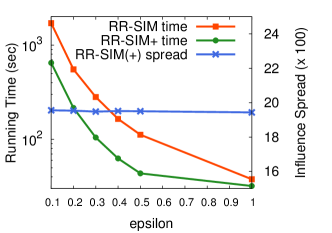
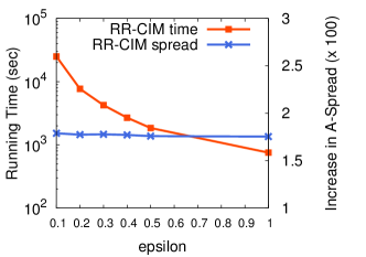
(a) SelfInfMax, Flixster	(b) CompInfMax, Flixster
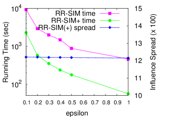
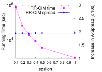
(c) SelfInfMax, Douban-Book	(d) CompInfMax, Douban-Book

Figure 4: Effects of $\epsilon$ on RR-set algorithms (Flixster and Douban-Book)

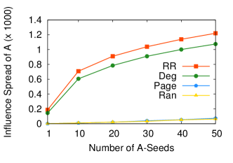
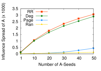
(a) Douban-Book	(b) Douban-Movie
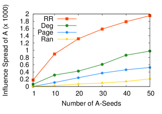
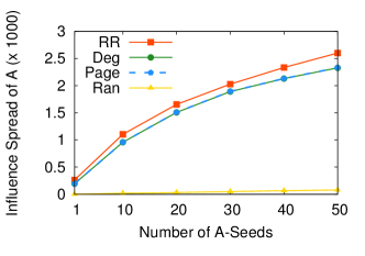
(c) Flixster	(d) Last.fm

Figure 5: $\mathcal{A}$-Spread vs. $|S_{\mathcal{A}}|$ for SelfInfMax (RR – $\mathsf{GeneralTIM}$ with $\mathsf{RR}$-$\mathsf{SIM}$+, Page – PageRank; Deg – High-Degree, Rand – Random)

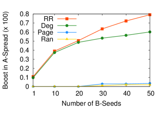
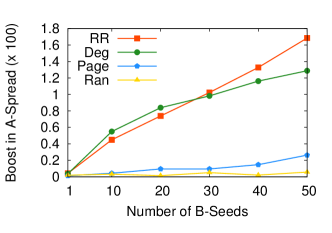
(a) Douban-Book, $\sigma_{\mathcal{A}}(S_{\mathcal{A}},\emptyset)=612$	(b) Douban-Movie, $\sigma_{\mathcal{A}}(S_{\mathcal{A}},\emptyset)=2357$
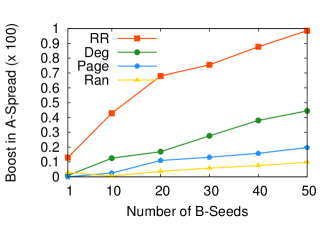
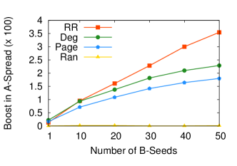
(c) Flixster, $\sigma_{\mathcal{A}}(S_{\mathcal{A}},\emptyset)=1643$	(d) Last.fm, $\sigma_{\mathcal{A}}(S_{\mathcal{A}},\emptyset)=1568$

Figure 6: Boost in $\mathcal{A}$-Spread vs. $|S_{\mathcal{B}}|$ for CompInfMax (RR – $\mathsf{GeneralTIM}$ with $\mathsf{RR}$-$\mathsf{CIM}$)

Effect of $\epsilon$ in $\mathsf{GeneralTIM}$

As mentioned in §6, $\epsilon$ controls the trade-off between approximation ratio and efficiency. Figure 4 plots influence spread and running time (log-scale) side-by-side, as a function of $\epsilon$, on Flixster and Douban-Book for both problems. The results on other datasets are very similar and thus omitted. We can see that as $\epsilon$ goes up from $0.1$ to $0.5$ and $1$ (in fact, $\epsilon=1>(1-1/e)$ means theoretical approximation guarantees are lost), the running time of all versions of $\mathsf{GeneralTIM}$ ($\mathsf{RR}$-$\mathsf{SIM}$, $\mathsf{RR}$-$\mathsf{SIM}$+, $\mathsf{RR}$-$\mathsf{CIM}$) decreases dramatically, by orders of magnitude. while, in practice, influence spread (SelfInfMax) and boost (CompInfMax) are almost completely unaffected (the largest difference among all test cases is only $0.45\%$).

Quality of Seeds

The quality of seeds is measured by the influence spread or boost achieved. We evaluate the spread of seed sets computed by all algorithms by MC simulations with 10K iterations for fair comparison. As can be seen from Figures 5 and 6, our RR-set algorithms are consistently the best in almost all test cases, often leading by a significant margin. The results of $\mathsf{Greedy}$ are omitted, since the spread it achieves is almost identical to $\mathsf{GeneralTIM}$, matching the observations in prior work [24]. $\mathsf{RR}$-$\mathsf{SIM}$ results are identical to $\mathsf{RR}$-$\mathsf{SIM}$+, and thus also omitted.

For SelfInfMax, $\mathsf{GeneralTIM}$ with $\mathsf{RR}$-$\mathsf{SIM}$+ is $13\%$, $2.7\%$, $100\%$, and $13\%$ better than the next best algorithm on Douban-Book, Douban-Movie, Flixster and Last.fm respectively, while for CompInfMax, $\mathsf{GeneralTIM}$ with $\mathsf{RR}$-$\mathsf{CIM}$ is $31\%$, $31\%$, $122\%$, and $51\%$ better. The boost in $\mathcal{A}$-spread provided by $\mathcal{B}$-seeds ($\mathsf{GeneralTIM}$ with $\mathsf{RR}$-$\mathsf{CIM}$) is at least $6\%$ to $15\%$ of the original $\mathcal{A}$-spread by $S_{\mathcal{A}}$ only. $\mathsf{HighDegree}$ performs well, especially in graphs with many nodes having large out-degrees (Douban-Movie, Last.fm), while $\mathsf{PageRank}$ produces good quality seeds only on Last.fm. $\mathsf{Random}$ is consistently the worst. The performances of baselines are generally consistent with observations in prior works [9, 10, 24] albeit for different diffusion models.

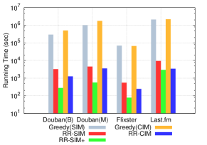
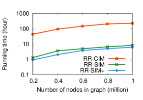
(a) Real networks	(b) Synthetic graphs

Figure 7: Running time

	Douban-Book	Douban-Movie	Flixster	Last.fm
$\mathsf{SIM_{learn}}$	$0.996$	$0.999$	$0.996$	$0.999$
$\mathsf{SIM_{0.1}}$	$0.652$	$0.962$	$0.492$	$0.519$
$\mathsf{SIM_{0.5}}$	$0.770$	$0.969$	$0.633$	$0.628$
$\mathsf{SIM_{0.9}}$	$0.946$	$0.985$	$0.926$	$0.879$
$\mathsf{CIM_{learn}}$	$0.973$	$0.918$	$0.950$	$0.825$
$\mathsf{CIM_{0.1}}$	$0.913$	$0.832$	$0.933$	$0.772$
$\mathsf{CIM_{0.5}}$	$0.936$	$0.885$	$0.969$	$0.857$
$\mathsf{CIM_{0.9}}$	$0.956$	$0.976$	$0.993$	$0.959$

Table 8: Sandwich approximation: $\sigma(S_{\nu})/\nu(S_{\nu})$

Running Time and Scalability

We compare the running time of $\mathsf{GeneralTIM}$ to $\mathsf{Greedy}$, shown in Figure 7(a). As can be seen, for SelfInfMax, $\mathsf{GeneralTIM}$ with $\mathsf{RR}$-$\mathsf{SIM}$, $\mathsf{RR}$-$\mathsf{SIM}$+ is about two to three orders of magnitude faster than $\mathsf{Greedy}$; for CompInfMax, $\mathsf{GeneralTIM}$ with $\mathsf{RR}$-$\mathsf{CIM}$ is also about two orders of magnitude faster than $\mathsf{Greedy}$. In addition, we observe that $\mathsf{RR}$-$\mathsf{SIM}$+ is 12, 8, 7, and 2 times as fast as $\mathsf{RR}$-$\mathsf{SIM}$ on Douban-Book, Douban-Movie, Flixster, and Last.fm respectively. The running time of $\mathsf{HighDegree}$, $\mathsf{PageRank}$, and $\mathsf{Random}$ baselines are omitted since they are typically very efficient [9, 10, 8].

We then use larger synthetic networks to test the scalability of $\mathsf{GeneralTIM}$ with our RR-set generation algorithms. We generate power-law random graphs of 0.2, 0.4, …, up to 1 million nodes with a power-law degree exponent of 2.16 [9]. These graphs have an average degree of about 5. We use the GPAs from Flixster. We can see that $\mathsf{GeneralTIM}$ with $\mathsf{RR}$-$\mathsf{SIM}$+ within 6.2 hours for the 1-million node graph, and its running time grows linearly in graph size, which indicates great scalability. $\mathsf{RR}$-$\mathsf{CIM}$ is slower due to the inherent intricacy of CompInfMax, but it also scales linearly. To put its running time measures in perspective, $\mathsf{Greedy}$— the only other known approximation algorithm for CompInfMax— takes about 48 hours on Flixster (12.9K nodes), while $\mathsf{GeneralTIM}$ with $\mathsf{RR}$-$\mathsf{CIM}$ is 4 hours faster on a graph 10 times as large.

Approximation Factors by Sandwich Approximation

Recall from §6.4 that the approximation factor yielded by SA is data-dependent: $\sigma(S_{\mathit{sand}})\geq\max\{\frac{\sigma(S_{\nu})}{\nu(S_{\nu})},\frac{\mu(S_{\sigma}^{*})}{\sigma(S_{\sigma}^{*})}\}\cdot(1-1/e-\epsilon)\cdot\sigma(S_{\sigma}^{*}).$ To see how good the SA approximation factor is in real-world graphs, we compute ${\sigma(S_{\nu})}/{\nu(S_{\nu})}$, as SA is guaranteed to have an approximation factor of at least $(1-1/e-\epsilon)\cdot{\sigma(S_{\nu})}/{\nu(S_{\nu})}$.

In the GAPs learned from data, both $q_{\mathcal{B}|\mathcal{A}}-q_{\mathcal{B}|\emptyset}$ and $q_{\mathcal{A}|\mathcal{B}}-q_{\mathcal{A}|\emptyset}$ are small and thus likely “friendly” to SA, as we mentioned in §6.4. Thus, we further “stress test” SA with more adversarial settings: First, set $q_{\mathcal{A}|\emptyset}=0.3$ and $q_{\mathcal{A}|\mathcal{B}}=0.8$; Then, for SelfInfMax, fix $q_{\mathcal{B}|\mathcal{A}}=1$ and vary $q_{\mathcal{B}|\emptyset}$ from $\{0.1,0.5,0.9\}$; for CompInfMax, fix $q_{\mathcal{B}|\emptyset}=0.1$ and vary $q_{\mathcal{B}|\mathcal{A}}$ from $\{0.1,0.5,0.9\}$.

Table 8 illustrates the results on all datasets with both learned GAPs and artificial GAPs. We use shorthands $\mathsf{SIM}$ and $\mathsf{CIM}$ for SelfInfMax and CompInfMax respectively. Subscript $\mathsf{learn}$ means the GAPs are learned from data. In stress-test cases (other six rows), e.g., for $\mathsf{SIM}$, subscript $\mathsf{0.5}$ means $q_{\mathcal{B}|\emptyset}=.5$, while for $\mathsf{CIM}$, it means $q_{\mathcal{B}|\mathcal{A}}=.5$. As can be seen, with real GAPs, the ratio is extremely close to $1$, matching our intuition. For artificial GAPs, the ratio is not as high, but most of them are still close to $1$. E.g., in the case of $\mathsf{SIM_{0.5}}$, $\sigma(S_{\nu})/\nu(S_{\nu})$ ranges from $0.628$ (Last.fm) to $0.969$ (Douban-Movie), which correspond to an approximation factor of $0.40$ and $0.61$ ($\epsilon$ omitted). Even the smallest ratio ($0.492$ in $\mathsf{SIM_{0.1}}$, Flixster) would still yield a decent factor at about $0.3$. This shows that SA is fairly effective and robust for solving non-submodular cases of SelfInfMax and CompInfMax.

We also measure the effectiveness of SA by comparing the spread achieved by seed sets $S_{\sigma},S_{\nu},S_{\mu}$ obtained w.r.t. the original, upper bound, and lower bound functions respectively. Such spread must be computed using the original function $\sigma$, and in our case, the unaltered GAPs. More specifically, we calculate the relative error defined as follows (for CompInfMax, disregard $S_{\mu}$).

$$\mathtt{SA\_error}=\frac{\max\{|\sigma(S_{\sigma})-\sigma(S_{\mu})|,|\sigma(S_{\sigma})-\sigma(S_{\nu})|\}}{\sigma(S_{\sigma})}.$$

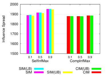
Figure 8: Sandwich Approximation on Flixster

In all four datasets, for both problems, the largest error is only $0.2\%$! To see if this is due to that $q_{\mathcal{B}|\emptyset}$ and $q_{\mathcal{B}|\mathcal{A}}$ being close in the GAPs learned from action log data, we further “stress test” SA with a much more adversarial set-up. For SelfInfMax, vary $q_{\mathcal{B}|\emptyset}$ to be $\{.1,.5,.9\}$ and fix $q_{\mathcal{B}|\mathcal{A}}=.96$. For CompInfMax, vary $q_{\mathcal{B}|\mathcal{A}}$ to be $\{.1,.5,.9\}$ and fix $q_{\mathcal{B}|\emptyset}=.1$ (to maintain complementarity). No change is made to $q_{\mathcal{A}|\emptyset}$ and $q_{\mathcal{A}|\mathcal{B}}$.

Figure 8 compares $\sigma(S_{\sigma})$, $\sigma(S_{\mu})$, and $\sigma(S_{\nu})$ on Flixster. As can be seen, even in this adversarial setting, SA is still highly effective for both SelfInfMax and CompInfMax. Amongst all test cases, the largest error is $0.4\%$. The results on other datasets are very similar and hence omitted.

8 Conclusions & Future Work

In this work, we propose the Comparative Independent Cascade (Com-IC) model that allows any degree of competition or complementarity between two different propagating items, and study the novel SelfInfMax and CompInfMax problems for complementary products. We develop non-trivial extensions to the RR-set techniques to achieve approximation algorithms. For non-submodular settings, we propose Sandwich Approximation to achieve data-dependent approximation factors. Our experiments demonstrate the effectiveness and efficiency of proposed solutions.

For future work, one direction is to design more efficient algorithms or heuristics for SelfInfMax and (especially) CompInfMax; e.g., whether near-linear time algorithm is still available for these problems is still open. Another direction is to fully characterize the entire GAP space $\mathbf{Q}$ in terms of monotonicity and submodularity properties. Moreover, an important direction is to extend the model to multiple items. Given the current framework, Com-IC can be extended to accommodate $k$ items, if we allow $k\cdot 2^{k-1}$ GAP parameters — for each item, we specify the probability of adoption for every combination of other items that have been adopted. However, how to simplify the model and make it tractable, how to reason about the complicated two-way or multi-way competition and complementarity, how to analyze monotonicity and submodularity, and how to learn GAP parameters from real-world data all remain as interesting challenges. Last, it is also interesting to consider an extended Com-IC model in which influence probabilities on edges are product-dependent.

Appendix

Appendix A Remarks on Com-IC Model

A.1 Unreachable States

Recall that in the Com-IC model, before an influence diffusion starts, all nodes are in the initial joint state ($\mathcal{A}$-idle, $\mathcal{B}$-idle). According to the diffusion dynamics defined in Figure 2, there exist five unreachable joint states, which are not material to our analysis and problem-solving, since none of these is relevant to actual adoptions, the objectives studied in SelfInfMax and CompInfMax. For completeness, we list these states here.

1. ($\mathcal{A}$-idle, $\mathcal{B}$-rejected)

2. ($\mathcal{A}$-suspended, $\mathcal{B}$-rejected)

3. ($\mathcal{A}$-rejected, $\mathcal{B}$-idle)

4. ($\mathcal{A}$-rejected, $\mathcal{B}$-suspended)

5. ($\mathcal{A}$-rejected, $\mathcal{B}$-rejected)

Lemma 9.

In any instance of the Com-IC model (no restriction on GAPs), no node can reach the state of ($\mathcal{A}$-idle, $\mathcal{B}$-rejected), from its initial state of ($\mathcal{A}$-idle, $\mathcal{B}$-idle).

Proof.

Let $v$ be an arbitrary node from graph $G=(V,E,p)$. Note that for $v$ to reject $\mathcal{B}$, it must be first be informed of $\mathcal{B}$ (otherwise it remains $\mathcal{B}$-idle, regardless of its state w.r.t. $\mathcal{A}$), and then becomes $\mathcal{B}$-suspended (otherwise it will be $\mathcal{B}$-adopted, a contradiction). Now, note that $v$ is never informed of $\mathcal{A}$, and hence it will not be triggered to reconsider $\mathcal{B}$, the only route to the state of $\mathcal{B}$-rejected, according to the model definition. Thus, ($\mathcal{A}$-idle, $\mathcal{B}$-rejected) is unreachable. ∎

The argument for ($\mathcal{A}$-rejected, $\mathcal{B}$-idle) being unreachable is symmetric, and hence omitted.

Lemma 10.

In any instance of the Com-IC model (no restriction on GAPs), no node can reach the state of ($\mathcal{A}$-suspended, $\mathcal{B}$-rejected), from its initial state of ($\mathcal{A}$-idle, $\mathcal{B}$-idle).

Proof.

Let $v$ be an arbitrary node from graph $G=(V,E,p)$. Note that for $v$ to reject $\mathcal{B}$, it must be first be informed of $\mathcal{B}$ (otherwise it remains $\mathcal{B}$-idle, regardless of its state w.r.t. $\mathcal{A}$), and then becomes $\mathcal{B}$-suspended (otherwise it will be $\mathcal{B}$-adopted, a contradiction). Now, $v$ transits from $\mathcal{A}$-idle to $\mathcal{A}$-suspended, meaning that $v$ does not adopt $\mathcal{A}$. This will not further trigger reconsideration, and hence $v$ stays at $\mathcal{B}$-suspended. This completes the proof. ∎

The argument for ($\mathcal{A}$-rejected, $\mathcal{A}$-suspended) being unreachable is symmetric, and hence omitted. Finally, it is evident from the proof of Lemma 10 that, the joint state of ($\mathcal{A}$-suspended, $\mathcal{A}$-suspended) is a sunken state, meaning the node will not get out it to adopt or reject any product. This implies that ($\mathcal{A}$-rejected, $\mathcal{B}$-rejected) is also unreachable.

A.2 Counter-Examples for Submodularity and Monotonicity

The first two counter-examples show that self-monotonicity and cross-monotonicity may not hold in general for the Com-IC model when there is no restriction on GAPs.

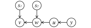
Figure 9: The graph for Example 1

Example 1 (Non-Self-Monotonicity).

Consider Figure 9. All edges have probability $1$. GAPs are $q_{\mathcal{A}|\emptyset}=q\in(0,1)$, $q_{\mathcal{A}|\mathcal{B}}=q_{\mathcal{B}|\emptyset}=1$, $q_{\mathcal{B}|\mathcal{A}}=0$, which means that $\mathcal{A}$ competes with $\mathcal{B}$ but $\mathcal{B}$ complements $\mathcal{A}$. Let $S_{\mathcal{B}}=\{y\}$. If $S_{\mathcal{A}}$ is $S=\{s_{1}\}$, the probability that $v$ becomes $\mathcal{A}$-adopted is $1$, because $v$ is informed of $\mathcal{A}$ from $s_{1}$, and even if it does not adopt $\mathcal{A}$ at the time, later it will surely adopt $\mathcal{B}$ propagated from $y$, and then $v$ will reconsider $\mathcal{A}$ and adopt $\mathcal{A}$. If it is $T=\{s_{1},s_{2}\}$, that probability is $1-q+q^{2}<1$: $w$ gets $\mathcal{A}$-adopted w.p. $q$ blocking $\mathcal{B}$ and then $v$ gets $\mathcal{A}$-adopted w.p. $q$; $w$ gets $\mathcal{B}$-adopted w.p. $(1-q)$ and then $v$ surely gets $\mathcal{A}$-adopted. Replicating sufficiently many $v$’s, all connected to $s_{1}$ and $w$, will lead to $\sigma_{\mathcal{A}}(T,S_{\mathcal{B}})<\sigma_{\mathcal{A}}(S,S_{B})$. The intuition is that the additional $\mathcal{A}$-seed $s_{2}$ “blocks” $\mathcal{B}$-propagation as $\mathcal{A}$ competes with $\mathcal{B}$ ($q_{\mathcal{B}|\mathcal{A}}<q_{\mathcal{B}|\emptyset}$) but $\mathcal{B}$ complements $\mathcal{A}$ ($q_{\mathcal{A}|\mathcal{B}}>q_{\mathcal{A}|\emptyset}$). Clearly $\sigma_{\mathcal{A}}$ is not monotonically decreasing in $S_{\mathcal{A}}$ either (e.g., in a graph when all nodes are isolated). Hence, $\sigma_{\mathcal{A}}$ is not monotone in $S_{\mathcal{A}}$. ∎

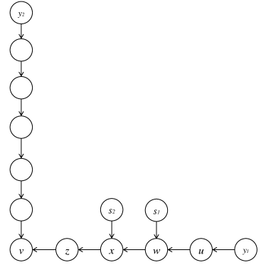
Figure 10: The graph for Example 2

Example 2 (Non-Cross-Monotonicity).

We use the example shown in Figure 10. All edges have probability $1$. Nodes $y_{1}$ and $y_{2}$ are the two fixed $\mathcal{A}$ seeds, and we want to grow $\mathcal{B}$ seed set from $S=\{s_{1}\}$ to $T=\{s_{1},s_{2}\}$. GAPs satisfy $0<q_{\mathcal{A}|\mathcal{B}}<q_{\mathcal{A}|\emptyset}<1$ and $0<q_{\mathcal{B}|\emptyset}<q_{\mathcal{B}|\mathcal{A}}<1$, which means that $\mathcal{A}$ complements $\mathcal{B}$ but $\mathcal{B}$ competes with $\mathcal{A}$. Since $\mathcal{B}$ competes with $\mathcal{A}$, it is straightforward to have examples in which the $\sigma_{\mathcal{A}}$ decreases when $\mathcal{B}$ seed set grows. We use Figure 10 to show a possible world in which the growth of $\mathcal{B}$ seed sets leads to $v$ adopting $\mathcal{A}$, indicating that $\mathcal{A}$ spread may also increase. Even though we do not have a direct example showing that $\sigma_{\mathcal{A}}$ increases when $\mathcal{B}$ seed set grows, we believe the possible world example is a good indication that $\sigma_{\mathcal{A}}$ is not cross-monotone in $S_{\mathcal{B}}$.

Figure 10 uses Figure 9 as a gadget. Intuitively, when $\mathcal{B}$ seed set grows from $S$ to $T$, the probability that $z$ adopts $B$ decreases as shown in Example 1. Then we utilize this and the fact that $\mathcal{B}$ competes with $\mathcal{A}$ to show that when $S$ is the $\mathcal{B}$ seed set, due to $\mathcal{B}$’s competition from $x$ node $v$ will not adopt $\mathcal{A}$, but when $T$ is the $\mathcal{B}$ seed set, there is no longer $\mathcal{B}$’s competition from $x$ and thus $v$ will adopt $\mathcal{A}$.

The node thresholds in the possible world are as follows: $q_{\mathcal{A}|\mathcal{B}}<\alpha^{w}_{\mathcal{A}}\leq q_{\mathcal{A}|\emptyset}$, $q_{\mathcal{B}|\emptyset}<\alpha^{x}_{\mathcal{B}}\leq q_{\mathcal{B}|\mathcal{A}}$, $q_{\mathcal{A}|\emptyset}<\alpha^{z}_{\mathcal{A}}$, $q_{\mathcal{A}|\mathcal{B}}<\alpha^{v}_{\mathcal{A}}\leq q_{\mathcal{A}|\emptyset}$, and all other non-specified $\alpha$ values take value $0$, meaning that they will not block diffusion.

Consider first that $S$ is the $\mathcal{B}$ seed set. Since $q_{\mathcal{B}|\emptyset}<\alpha^{x}_{\mathcal{B}}$, $x$ is informed about $\mathcal{B}$ from $s_{1}$ but will not adopt $\mathcal{B}$ directly from $s_{1}$. From $y_{1}$, we can see that $\mathcal{A}$ will pass through $u$, $w$ and reaches $x$. After $x$ adopts $\mathcal{A}$, it reconsiders $\mathcal{B}$, and since $\alpha^{x}_{\mathcal{B}}\leq q_{\mathcal{B}|\mathcal{A}}$, $x$ adopts $\mathcal{B}$. Node $x$ then informs $z$ about $\mathcal{A}$ and $\mathcal{B}$, in this order. However, since $q_{\mathcal{A}|\emptyset}<\alpha^{z}_{\mathcal{A}}$, $z$ does not adopt $\mathcal{A}$, but it adopts $\mathcal{B}$ ($\alpha^{z}_{\mathcal{B}}=0\leq q_{\mathcal{B}|\emptyset}$). Next $z$ informs $v$ about $\mathcal{B}$, which adopts $\mathcal{B}$ since $\alpha^{v}_{\mathcal{B}}=0\leq q_{\mathcal{B}|\emptyset}$. This happens one step earlier than $\mathcal{A}$ reaches $v$ from $y_{2}$, but since $q_{\mathcal{A}|\mathcal{B}}<\alpha^{v}_{\mathcal{A}}$, $v$ will not adopt $\mathcal{A}$.

Now consider that $T$ is the $\mathcal{B}$ seed set. In this case, $w$ definitely adopts $\mathcal{B}$ from $s_{2}$. Since $q_{\mathcal{A}|\mathcal{B}}<\alpha^{w}_{\mathcal{A}}$ and $w$ adopts $\mathcal{B}$ first, $w$ will not adopt $\mathcal{A}$ from $y_{1}$. Because $q_{\mathcal{B}|\emptyset}<\alpha^{x}_{\mathcal{B}}$ and $w$ blocks $\mathcal{A}$ from reaching $x$, $x$ will not adopt $\mathcal{A}$ or $\mathcal{B}$. Then $z$ will not adopt $\mathcal{A}$ or $\mathcal{B}$ either. This allows $\mathcal{A}$ to reach $v$ from $y_{2}$, and since $q_{\mathcal{A}|\mathcal{B}}<\alpha^{v}_{\mathcal{A}}\leq q_{\mathcal{A}|\emptyset}$, $v$ adopts $\mathcal{A}$.

We can certainly duplicate $v$ enough times so that when $\mathcal{B}$ seed set grows from $S$ to $T$, the $\mathcal{A}$-spread in this possible world also increases, even though $\mathcal{B}$ is competing with $\mathcal{A}$. ∎

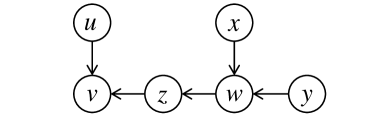
Figure 11: The graph for Example 3 and 4

The following two examples show that even when two items are mutually complementary, self-submodularity and cross-submodularity in general may not hold.

Example 3 (Non-Self-Submodularity).

Consider the possible world in Figure 11. All edges are live. The node thresholds are: for $w$: $\alpha_{\mathcal{A}}^{w}\leq q_{\mathcal{A}|\emptyset}$, $q_{\mathcal{B}|\emptyset}<\alpha_{\mathcal{B}}^{w}\leq q_{\mathcal{B}|\mathcal{A}}$; for $z$: $\alpha_{\mathcal{A}}^{z}>q_{\mathcal{A}|\mathcal{B}}$, $\alpha_{\mathcal{B}}^{z}<q_{\mathcal{B}|\emptyset}$; for $v$: $q_{\mathcal{A}|\emptyset}<\alpha_{\mathcal{A}}^{v}\leq q_{\mathcal{A}|\mathcal{B}}$, $\alpha_{\mathcal{B}}^{v}\leq q_{\mathcal{B}|\emptyset}$; Then fix $S_{\mathcal{B}}=\{y\}$. For $S_{\mathcal{A}}$, let $S=\emptyset$, $T=\{x\}$, and $u$ is the additional seed. It can be verified that only when $S_{\mathcal{A}}=T\cup\{u\}$, $v$ becomes $\mathcal{A}$-adopted, violating self-submodularity.

A concrete example of $\mathbf{Q}$ for which submodularity does not hold is as follows: $q_{\mathcal{A}|\emptyset}=0.078432$; $q_{\mathcal{A}|\mathcal{B}}=0.24392$; $q_{\mathcal{B}|\emptyset}=0.37556$; $q_{\mathcal{B}|\mathcal{A}}=0.99545$. Seed sets are the same as above. We denote by $p_{v}(S_{\mathcal{A}})$ the probability that $v$ becomes $\mathcal{A}$-adopted with A-seed set $S_{\mathcal{A}}$. It can be verified that: $p_{v}(S)=0$, $p_{v}(S\cup\{u\})=8.898\cdot 10^{-5}$, $p_{v}(T)=0.027254$, and $p_{v}(T\cup\{u\})=0.027383$. Clearly, $p_{v}(T\cup\{u\})-p_{v}(T)>p_{v}(S\cup\{u\})-p_{v}(S)$. Hence, replicating $v$ sufficiently many times will lead to $\sigma_{\mathcal{A}}(T\cup\{u\},S_{\mathcal{B}})-\sigma_{\mathcal{A}}(T,S_{\mathcal{B}})\geq\sigma_{\mathcal{A}}(S\cup\{u\},S_{\mathcal{B}})-\sigma_{\mathcal{A}}(S,S_{\mathcal{B}})$, violating self-submodularity. ∎

Example 4 (Non-Cross-Submodularity).

Consider the possible world in Figure 11. The node thresholds are: For $w$: $q_{\mathcal{A}|\emptyset}<\alpha_{\mathcal{A}}^{w}\leq q_{\mathcal{A}|\mathcal{B}}$, $\alpha_{\mathcal{B}}^{w}\leq q_{\mathcal{B}|\emptyset}$; for $z$: $\alpha_{\mathcal{A}}^{z}\leq q_{\mathcal{A}|\emptyset}$, $\alpha_{\mathcal{B}}^{z}>q_{\mathcal{B}|\mathcal{A}}$; for $v$: $q_{\mathcal{A}|\emptyset}<\alpha_{\mathcal{A}}^{v}\leq q_{\mathcal{A}|\mathcal{B}}$, $\alpha_{\mathcal{B}}^{v}\leq q_{\mathcal{B}|\emptyset}$. Fix $S_{\mathcal{A}}=\{y\}$. For $S_{\mathcal{B}}$, let $S=\emptyset$, $T=\{x\}$, and $u$ is the additional seed. It can be verified that only when $S_{\mathcal{B}}=T\cup\{u\}$, $v$ becomes $\mathcal{A}$-adopted, violating cross-submodularity. ∎

The above example applies even when $q_{\mathcal{B}|\mathcal{A}}=q_{\mathcal{B}|\emptyset}<1$. The key is that $q_{\mathcal{B}|\mathcal{A}}<1$ and $\alpha_{\mathcal{B}}^{z}>q_{\mathcal{B}|\mathcal{A}}$, which prevents $\mathcal{B}$ to pass through $z$, and thus another $\mathcal{B}$-seed $u$ is needed to inform $v$ of $\mathcal{B}$.

Appendix B Proofs and Additional Theoretical Results

B.1 Proofs for Results in Section 4

Theorem 2 (re-stated). For CompInfMax, when $q_{\mathcal{B}|\emptyset}=1$ and $k\geq|S_{\mathcal{A}}|$, we can solve the problem optimally by setting $S_{\mathcal{B}}^{*}$ to be $S_{\mathcal{A}}\cup X$, where $X$ is an arbitrary set in $V\setminus S_{\mathcal{A}}$ with size $k-|S_{\mathcal{A}}|$, that is $\sigma_{\mathcal{A}}(S_{\mathcal{A}},S_{\mathcal{A}}\cup X)=\max_{T\subseteq V,|T|=k}\sigma_{\mathcal{A}}(S_{\mathcal{A}},T)$.

Proof.

We first show the theorem holds in an arbitrary possible world $W$. Following Eq. (4), when $S_{\mathcal{A}}$ acts alone (without any $\mathcal{B}$-seeds), we can classify all nodes into four types: $\mathcal{A}$-adopted, $\mathcal{A}$-rejected, $\mathcal{A}$-suspended, and $\mathcal{A}$-potential. Clearly, only $\mathcal{A}$-suspended and $\mathcal{A}$-potential may later adopt $\mathcal{A}$ with the help of $\mathcal{B}$, and the other two types are not relevant to CompInfMax.

Now, let all nodes in $S_{\mathcal{A}}$ be $\mathcal{B}$-seeds, and thus they become $\mathcal{B}$-adopted, too. Since $q_{\mathcal{B}|\emptyset}=1$, all nodes that can be reached by the seeds via live-edge paths will eventually become $\mathcal{B}$-adopted, including all $\mathcal{A}$-suspended and $\mathcal{A}$-potential nodes. For $\mathcal{A}$-suspended nodes, after adopting $\mathcal{B}$, they will adopt $\mathcal{A}$ through re-consideration right away. For $\mathcal{A}$-potential nodes, the propagation of $\mathcal{A}$ will reach them after $\mathcal{A}$-suspended nodes upstream adopt $\mathcal{A}$ (together with $\mathcal{B}$), and after being reached, they adopt both items.

Therefore, in this possible world, making $S_{\mathcal{A}}$ to be $\mathcal{B}$-seeds will “convert” all nodes that can possibly become $\mathcal{A}$-adopted, namely all $\mathcal{A}$-suspended and $\mathcal{A}$-potential nodes. Hence, any additional $\mathcal{B}$-seed will not further increase the spread of $\mathcal{A}$ as no other nodes can possibly be “converted”.

Since the claim in this theorem holds true for any arbitrary possible world $W$, it also holds for all other possible worlds that belong to the same equivalence class $\bf W$. Since

$$\sigma_{\mathcal{A}}(S_{\mathcal{A}},S_{\mathcal{B}})=\sum_{\bf W}\Pr[\mathbf{W}]\sigma_{\mathcal{A}}^{\mathbf{W}}(S_{\mathcal{A}},S_{\mathcal{B}}),$$

the theorem is proven. ∎

B.2 Proofs for Results in Section 5

Lemma 1 (re-stated). For any fixed $\mathcal{A}$-seed set $S_{\mathcal{A}}$ and $\mathcal{B}$-seed set $S_{\mathcal{B}}$, the joint distributions of the sets of $\mathcal{A}$-adopted nodes and $\mathcal{B}$-adopted nodes obtained $(i)$ by running a Com-IC diffusion from $S_{\mathcal{A}}$ and $S_{\mathcal{B}}$ and $(ii)$ by randomly sampling a possible world $W$ and running a deterministic cascade from $S_{\mathcal{A}}$ and $S_{\mathcal{B}}$ in $W$, are the same.

Proof.

The proof is based on establishing equivalence on all edge-level and node-level behaviors in Com-IC and the PW model. By the principle of deferred decisions and the fact that each edge is only tested once in one diffusion, edge transition processes are equivalent. To generate a possible world, the live/blocked status of an edge is pre-determined and revealed when needed, while in a Com-IC process, the status is determined on-the-fly.

Tie-breaking is also equivalent. Note that each node $v$ only needs to apply the random permutation $\pi_{v}$ for breaking ties at most once. For Com-IC, we need to apply $\pi_{v}$ only when $v$ is transitioning out of state ($\mathcal{A}$-idle, $\mathcal{B}$-idle) after being informed of both $\mathcal{A}$ and $\mathcal{B}$. Clearly, this transition occurs at most once for each node. The same logic applies to the PW model. Thus, the equivalence is obvious due to the principle of deferred decisions.

The equivalence of decision-making for adoption is straightforward as $\alpha_{\mathcal{A}}^{v}$ and $\alpha_{\mathcal{B}}^{v}$ are chosen uniformly at random from $[0,1]$. Hence, $\Pr[\alpha_{\mathcal{A}}^{v}\leq q]=q$, where $q\in\{q_{\mathcal{A}|\emptyset},q_{\mathcal{A}|\mathcal{B}},q_{\mathcal{B}|\emptyset},q_{\mathcal{B}|\mathcal{A}}\}$.

As to reconsideration, w.l.o.g. we consider $\mathcal{A}$. In Com-IC, the probability of reconsideration is $\rho_{\mathcal{A}}=\max\{(q_{\mathcal{A}|\mathcal{B}}-q_{\mathcal{A}|\emptyset}),0\}/(1-q_{\mathcal{A}|\emptyset})$. In PW, when $q_{\mathcal{A}|\mathcal{B}}\geq q_{\mathcal{A}|\emptyset}$, this amounts to the probability that $\alpha_{\mathcal{A}}^{v}\leq q_{\mathcal{A}|\mathcal{B}}$ given $\alpha_{\mathcal{A}}^{v}>q_{\mathcal{A}|\emptyset}$, which is $(q_{\mathcal{A}|\mathcal{B}}-q_{\mathcal{A}|\emptyset})/(1-q_{\mathcal{A}|\emptyset})$. On the other hand, when $q_{\mathcal{A}|\mathcal{B}}<q_{\mathcal{A}|\emptyset}$, $\alpha_{\mathcal{A}}^{v}>q_{\mathcal{A}|\emptyset}$ implies $\alpha_{\mathcal{A}}^{v}>q_{\mathcal{A}|\mathcal{B}}$, which means reconsideration is meaningless, and this corresponds to $\rho_{\mathcal{A}}=0$ in Com-IC. Thus, the equivalence is established.

Finally, the seeding protocol is trivially the same. Combining the equivalence for all edge-level and node-level activities, we can see that the two models are equivalent and yield the same distribution of $\mathcal{A}$- and $\mathcal{B}$-adopted nodes, for any given $S_{\mathcal{A}}$ and $S_{\mathcal{B}}$. ∎

Theorem 3 (re-stated). For any fixed $\mathcal{B}$-seed set $S_{\mathcal{B}}$, $\sigma_{\mathcal{A}}(S_{\mathcal{A}},S_{\mathcal{B}})$ is monotonically increasing in $S_{\mathcal{A}}$ for any set of GAPs in $\mathbf{Q}^{+}$ and $\mathbf{Q}^{-}$. Also, $\sigma_{\mathcal{A}}(S_{\mathcal{A}},S_{\mathcal{B}})$ is monotonically increasing in $S_{\mathcal{B}}$ for any GAPs in $\mathbf{Q}^{+}$, and monotonically decreasing in $S_{\mathcal{B}}$ for any $\mathbf{Q}^{-}$.

For ease of exposition, we also state a symmetric version of Theorem 3 w.r.t. $\sigma_{\mathcal{B}}$. That is, given any fixed $\mathcal{A}$-seed set, $\sigma_{\mathcal{B}}(S_{\mathcal{A}},S_{\mathcal{B}})$ is monotonically increasing in $S_{\mathcal{B}}$ for any set of GAPs in $\mathbf{Q}^{+}$ and $\mathbf{Q}^{-}$. Also, $\sigma_{\mathcal{B}}(S_{\mathcal{A}},S_{\mathcal{B}})$ is monotonically increasing in $S_{\mathcal{A}}$ for any GAPs in $\mathbf{Q}^{+}$, and monotonically decreasing in $S_{\mathcal{A}}$ for any $\mathbf{Q}^{-}$. For technical reasons and notational convenience, in the proof of Theorem 3 presented below, we “concurrently” prove both Theorem 3 and this symmetric version, without loss of generality.

Proof of Theorem 3.

We first fix a $\mathcal{B}$-seed set $S_{\mathcal{B}}$. Since $S_{\mathcal{B}}$ is always fixed, in the remaining proof we ignore $S_{\mathcal{B}}$ from the notations whenever it is clear from context. It suffices to show that monotonicity holds in an arbitrary, fixed possible world, which implies monotonicity holds for the diffusion model. Let $W$ be an arbitrary possible world generated according to §5.1.

Define $\Phi_{\mathcal{A}}^{W}(S_{\mathcal{A}})$ (resp. $\Phi_{\mathcal{B}}^{W}(S_{\mathcal{A}})$) to be the set of $\mathcal{A}$-adopted (resp. $\mathcal{B}$-adopted) nodes in possible world $W$ with $S_{\mathcal{A}}$ being the $\mathcal{A}$-seed set (and $S_{\mathcal{B}}$ being the fixed $\mathcal{B}$-seed set). Furthermore, for any time step $t\geq 0$, define $\Phi_{\mathcal{A}}^{W}(S_{\mathcal{A}},t)$ (resp. $\Phi_{\mathcal{B}}^{W}(S_{\mathcal{A}},t)$) to be the set of $\mathcal{A}$-adopted (resp. $\mathcal{B}$-adopted) nodes in $W$ by the end of step $t$, given $\mathcal{A}$-seed set $S_{\mathcal{A}}$. Clearly, $\Phi_{\mathcal{A}}^{W}(S_{\mathcal{A}})=\cup_{t\geq 0}\Phi_{\mathcal{A}}^{W}(S_{\mathcal{A}},t)$ and $\Phi_{\mathcal{B}}^{W}(S_{\mathcal{A}})=\cup_{t\geq 0}\Phi_{\mathcal{B}}^{W}(S_{\mathcal{A}},t)$. Let $S$ and $T$ be two sets, with $S\subseteq T\subseteq V$.

Mutual Competition $\mathbf{Q}^{-}$. Our goal is to prove that for any $v\in V$, (a) if $v\in\Phi_{\mathcal{A}}^{W}(S)$, then $v\in\Phi_{\mathcal{A}}^{W}(T)$; and (b) if $v\in\Phi_{\mathcal{B}}^{W}(T)$, then $v\in\Phi_{\mathcal{B}}^{W}(S)$. Item (a) implies self-monotonic increasing property while item (b) implies cross-monotonic decreasing property. We use an inductive proof to combine the proof of above two results together, as follows. For every $t\geq 0$, we inductively show that $(i)$ if $v\in\Phi_{\mathcal{A}}^{W}(S,t)$, then $v\in\Phi_{\mathcal{A}}^{W}(T,t)$; and $(ii)$ if $v\in\Phi_{\mathcal{B}}^{W}(T,t)$, then $v\in\Phi_{\mathcal{B}}^{W}(S,t)$.

Consider the base case of $t=0$. If $v\in\Phi_{\mathcal{A}}^{W}(S,0)$, then it means $v\in S$, and thus $v\in T=\Phi_{\mathcal{A}}^{W}(T,0)$. If $v\in\Phi_{\mathcal{B}}^{W}(T,0)$, it means $v\in S_{\mathcal{B}}$, and thus $v\in\Phi_{\mathcal{B}}^{W}(S,0)=S_{\mathcal{B}}$.

For the induction step, suppose that for all $t<t$, $(i)$ and $(ii)$ hold, and we show $(i)$ and $(ii)$ also hold for $t=t^{\prime}$. For $(i)$, we only need to consider $v\in\Phi_{\mathcal{A}}^{W}(S,t^{\prime})\setminus\Phi_{\mathcal{A}}^{W}(S,t^{\prime}-1)$, i.e. $v$ adopts $\mathcal{A}$ at step $t^{\prime}$ when $S$ is the $\mathcal{A}$-seed set. Since $v$ adopts $\mathcal{A}$, we know that $\alpha_{\mathcal{A}}^{v}\leq q_{\mathcal{A}|\emptyset}$. Let $U$ be the set of in-neighbors of $v$ in the possible world $W$. Let $U_{\mathcal{A}}(S_{\mathcal{A}})=U\cap\Phi_{\mathcal{A}}^{W}(S_{\mathcal{A}},t^{\prime}-1)$ and $U_{\mathcal{B}}(S_{\mathcal{A}})=U\cap\Phi_{\mathcal{B}}^{W}(S_{\mathcal{A}},t^{\prime}-1)$, i.e. $U_{\mathcal{A}}(S_{\mathcal{A}})$ (resp. $U_{\mathcal{B}}(S_{\mathcal{A}})$) is the set of in-neighbors of $v$ in $W$ that adopted $\mathcal{A}$ (resp. $\mathcal{B}$) by time $t^{\prime}-1$, when $S_{\mathcal{A}}$ is the $\mathcal{A}$-seed set. Since $v\in\Phi_{\mathcal{A}}^{W}(S,t^{\prime})$, we know that $U_{\mathcal{A}}(S)\neq\emptyset$. By induction hypothesis, we have $U_{\mathcal{A}}(S)\subseteq U_{\mathcal{A}}(T)$ and $U_{\mathcal{B}}(T)\subseteq U_{\mathcal{B}}(S)$.

Thus, $U_{\mathcal{A}}(T)\neq\emptyset$, which implies that by step $t^{\prime}$, $v$ must have been informed of $\mathcal{A}$ when $T$ is the $\mathcal{A}$-seed set. If $\alpha_{\mathcal{A}}^{v}\leq q_{\mathcal{A}|\mathcal{B}}$, then no matter if $v$ adopted $\mathcal{B}$ or not, $v$ would adopt $\mathcal{A}$ by step $t^{\prime}$ according to the possible world model. That is, $v\in\Phi_{\mathcal{A}}^{W}(T,t^{\prime})$.

Now suppose $q_{\mathcal{A}|\mathcal{B}}<\alpha_{\mathcal{A}}^{v}\leq q_{\mathcal{A}|\emptyset}$. For a contradiction suppose $v\not\in\Phi_{\mathcal{A}}^{W}(T,t^{\prime})$, i.e., $v$ does not adopt $\mathcal{A}$ by step $t^{\prime}$ when $T$ is the $\mathcal{A}$-seed set. Since $v$ has been informed of $\mathcal{A}$ by $t^{\prime}$, the only possibility that $v$ does not adopt $\mathcal{A}$ is because $v$ adopted $\mathcal{B}$ earlier than $\mathcal{A}$, which means $v\in\Phi_{\mathcal{B}}^{W}(T,t^{\prime})$. Two cases arise:

First, if $v\in\Phi_{\mathcal{B}}^{W}(T,t^{\prime}-1)$, then by the induction hypothesis $v\in\Phi_{\mathcal{B}}^{W}(S,t^{\prime}-1)$. Since $v\in\Phi_{\mathcal{A}}^{W}(S,t^{\prime})\setminus\Phi_{\mathcal{A}}^{W}(S,t^{\prime}-1)$, it means that when $S$ is the $\mathcal{A}$-seed set, $v$ adopts $\mathcal{B}$ first before adopting $\mathcal{A}$, but this contradicts to the condition that $q_{\mathcal{A}|\mathcal{B}}<\alpha_{\mathcal{A}}^{v}$. Therefore, $v\not\in\Phi_{\mathcal{B}}^{W}(T,t^{\prime}-1)$.

Second, $v\in\Phi_{\mathcal{B}}^{W}(T,t^{\prime})\setminus\Phi_{\mathcal{B}}^{W}(T,t^{\prime}-1)$. Since $v\not\in\Phi_{\mathcal{A}}^{W}(T,t^{\prime})$, it means that $v$ is informed of $\mathcal{A}$ at step $t^{\prime}$ when $T$ is the $\mathcal{A}$-seed set, and thus the tie-breaking rule must have been applied at this step and $\mathcal{B}$ is ordered first before $\mathcal{A}$. However, looking at the in-neighbors of $v$ in $W$, by the induction hypothesis, $U_{\mathcal{A}}(S)\subseteq U_{\mathcal{A}}(T)$ and $U_{\mathcal{B}}(T)\subseteq U_{\mathcal{B}}(S)$. This implies that when $S$ is the $\mathcal{A}$-seed set, the same tie-breaking rule at $\mathcal{A}$ would still order $\mathcal{B}$ first before $\mathcal{A}$, but this would result in $v$ not adopting $\mathcal{A}$ at step $t^{\prime}$, a contradiction. Therefore, we know that $v\in\Phi_{\mathcal{A}}^{W}(T,t^{\prime})$.

The statement of $(ii)$ is symmetric to $(i)$: if we exchange $\mathcal{A}$ and $\mathcal{B}$ and exchange $S$ and $T$, $(ii)$ becomes $(i)$. In fact, one can check that we can literally translate the induction step proof for $(i)$ into the proof for $(ii)$ by exchanging pair $\mathcal{A}$ and $\mathcal{B}$ and pair $S$ and $T$ (except that (a) we keep the definitions of $U_{\mathcal{A}}(S_{\mathcal{A}})$ and $U_{\mathcal{B}}(S_{\mathcal{A}})$, and (b) whenever we say some set is the $\mathcal{A}$-seed set, we keep this $\mathcal{A}$). This concludes the proof of the mutual competition case.

Mutual Complementarity $\mathbf{Q}^{+}$. The proof structure is very similar to that of the mutual competition case. Our goal is to prove that for any $v\in V$, (a) if $v\in\Phi_{\mathcal{A}}^{W}(S)$, then $v\in\Phi_{\mathcal{A}}^{W}(T)$; and (b) if $v\in\Phi_{\mathcal{B}}^{W}(S)$, then $v\in\Phi_{\mathcal{B}}^{W}(T)$. To show this, we inductively prove the following: For every $t\geq 0$, $(i)$ if $v\in\Phi_{\mathcal{A}}^{W}(S,t)$, then $v\in\Phi_{\mathcal{A}}^{W}(T,t)$; and $(ii)$ if $v\in\Phi_{\mathcal{B}}^{W}(S,t)$, then $v\in\Phi_{\mathcal{B}}^{W}(T,t)$. The base case is trivially true.

For the induction step, suppose $(i)$ and $(ii)$ hold for all $t<t^{\prime}$, and we show that $(i)$ and $(ii)$ also hold for $t=t^{\prime}$.

For $(i)$, we only need to consider $v\in\Phi_{\mathcal{A}}^{W}(S,t^{\prime})\setminus\Phi_{\mathcal{A}}^{W}(S,t^{\prime}-1)$, i.e. $v$ adopts $\mathcal{A}$ at step $t^{\prime}$ when $S$ is the $\mathcal{A}$-seed set. Since $v$ adopts $\mathcal{A}$, we know that $\alpha_{\mathcal{A}}^{v}\leq q_{\mathcal{A}|\mathcal{B}}$. Since $v\in\Phi_{\mathcal{A}}^{W}(S,t^{\prime})$, we know that $U_{\mathcal{A}}(S)\neq\emptyset$. By induction hypothesis we have $U_{\mathcal{A}}(S)\subseteq U_{\mathcal{A}}(T)$. Thus we know that $U_{\mathcal{A}}(T)\neq\emptyset$, which implies that by step $t^{\prime}$, $v$ must have been informed of $\mathcal{A}$ when $T$ is the $\mathcal{A}$-seed set. if $\alpha_{\mathcal{A}}^{v}\leq q_{\mathcal{A}|\emptyset}$, then no matter $v$ adopted $\mathcal{B}$ or not, $v$ would adopt $\mathcal{A}$ by step $t^{\prime}$ according to the possible world model. Thus, $v\in\Phi_{\mathcal{A}}^{W}(T,t^{\prime})$.

Now suppose $q_{\mathcal{A}|\emptyset}<\alpha_{\mathcal{A}}^{v}\leq q_{\mathcal{A}|\mathcal{B}}$. Since $v\in\Phi_{\mathcal{A}}^{W}(S,t^{\prime})$, the only possibility is that $v$ adopts $\mathcal{B}$ first by time $t^{\prime}$ so that after reconsideration, $v$ adopts $\mathcal{A}$ due to condition $\alpha_{\mathcal{A}}^{v}\leq q_{\mathcal{A}|\mathcal{B}}$. Thus we have $v\in\Phi_{\mathcal{B}}^{W}(S,t^{\prime})$, and $\alpha_{\mathcal{B}}^{v}\leq q_{\mathcal{B}|\emptyset}$.

If $v\in\Phi_{\mathcal{B}}^{W}(S,t^{\prime}-1)$, by induction hypothesis $v\in\Phi_{\mathcal{B}}^{W}(T,t^{\prime}-1)$, which means that $v$ adopts $\mathcal{B}$ by time $t^{\prime}-1$ when $T$ is the $\mathcal{A}$-seed set. Since $v$ has been informed of $\mathcal{A}$ by time $t^{\prime}$ when $T$ is the $\mathcal{A}$-seed set, condition $\alpha_{\mathcal{A}}^{v}\leq q_{\mathcal{A}|\mathcal{B}}$ implies that $v$ adopts $\mathcal{A}$ by time $t^{\prime}$ when $T$ is the $\mathcal{A}$-seed set, i.e. $v\in\Phi_{\mathcal{A}}^{W}(T,t^{\prime})$.

Finally we consider the case of $v\in\Phi_{\mathcal{B}}^{W}(S,t^{\prime})\setminus\Phi_{\mathcal{B}}^{W}(S,t^{\prime}-1)$. Looking at the in-neighbors of $v$ in $W$, $v\in\Phi_{\mathcal{B}}^{W}(S,t^{\prime})$, implies that $U_{\mathcal{B}}(S)\neq\emptyset$. By the induction hypothesis, we have $U_{\mathcal{B}}(S)\subseteq U_{\mathcal{B}}(T)$, and thus $U_{\mathcal{B}}(T)\neq\emptyset$. This implies that when $T$ is the $\mathcal{A}$-seed set, node $v$ must have been informed of $\mathcal{B}$ by time $t^{\prime}$. Since $\alpha_{\mathcal{B}}^{v}\leq q_{\mathcal{B}|\emptyset}$, we have that $v$ adopts $\mathcal{B}$ by time $t^{\prime}$ when $T$ is the $\mathcal{A}$-seed set. Then the condition $\alpha_{\mathcal{A}}^{v}\leq q_{\mathcal{A}|\mathcal{B}}$ implies that $v$ adopts $\mathcal{A}$ by time $t^{\prime}$ when $T$ is the $\mathcal{A}$-seed set, i.e. $v\in\Phi_{\mathcal{A}}^{W}(T,t^{\prime})$.

This concludes the inductive step for item $(i)$ in the mutual complementarity case. The induction step for item $(ii)$ is completely symmetric to the inductive step for item $(i)$. Therefore, we complete the proof for the mutual complementarity case. As a result, the whole theorem holds. ∎

Lemma 2 (re-stated). Consider any Com-IC instance with $\mathbf{Q}^{+}$. Given fixed $\mathcal{A}$- and $\mathcal{B}$-seed sets, for all nodes $v\in V$, all permutations of $v$’s in-neighbors are equivalent in determining if $v$ becomes $\mathcal{A}$-adopted and $\mathcal{B}$-adopted, and thus the tie-breaking rule is not needed for mutual complementary case.

Proof.

Without loss of generality, we only need to consider a node $v$ and two of its in-neighbours $u_{\mathcal{A}}$ and $u_{\mathcal{B}}$ which become $\mathcal{A}$-adopted and $\mathcal{B}$-adopted at $t-1$ respectively. In a possible world, there are nine possible combinations of the values of $\alpha_{\mathcal{A}}^{v}$ and $\alpha_{\mathcal{B}}^{v}$. We show that in all such combinations, the ordering $\pi_{1}=\langle u_{\mathcal{A}},u_{\mathcal{B}}\rangle$ and $\pi_{2}=\langle u_{\mathcal{B}},u_{\mathcal{A}}\rangle$ produce the same outcome for $v$.

1. $\alpha_{\mathcal{A}}^{v}\leq q_{\mathcal{A}|\emptyset}\wedge\alpha_{\mathcal{B}}^{v}\leq q_{\mathcal{B}|\emptyset}$. Both $\pi_{1}$ and $\pi_{2}$ make $v$ $\mathcal{A}$-adopted and $\mathcal{B}$-adopted.

2. $\alpha_{\mathcal{A}}^{v}\leq q_{\mathcal{A}|\emptyset}\wedge q_{\mathcal{B}|\emptyset}<\alpha_{\mathcal{B}}^{v}\leq q_{\mathcal{B}|\mathcal{A}}$. Both $\pi_{1}$ and $\pi_{2}$ make $v$ $\mathcal{A}$-adopted and $\mathcal{B}$-adopted. With $\pi_{2}$, $v$ first becomes $\mathcal{B}$-suspended, then $\mathcal{A}$-adopted, and finally $\mathcal{B}$-adopted due to re-consideration.

3. $\alpha_{\mathcal{A}}^{v}\leq q_{\mathcal{A}|\emptyset}\wedge\alpha_{\mathcal{B}}^{v}>q_{\mathcal{B}|\mathcal{A}}$. Both $\pi_{1}$ and $\pi_{2}$ makes $v$ $\mathcal{A}$-adopted only.

4. $q_{\mathcal{A}|\emptyset}<\alpha_{\mathcal{A}}^{v}\leq q_{\mathcal{A}|\mathcal{B}}\wedge\alpha_{\mathcal{B}}^{v}\leq q_{\mathcal{B}|\emptyset}$. Symmetric to case 2 above.

5. $q_{\mathcal{A}|\emptyset}<\alpha_{\mathcal{A}}^{v}\leq q_{\mathcal{A}|\mathcal{B}}\wedge q_{\mathcal{B}|\emptyset}<\alpha_{\mathcal{B}}^{v}\leq q_{\mathcal{B}|\mathcal{A}}$. In this case, $v$ does not adopt any item.

6. $q_{\mathcal{A}|\emptyset}<\alpha_{\mathcal{A}}^{v}\leq q_{\mathcal{A}|\mathcal{B}}\wedge\alpha_{\mathcal{B}}^{v}>q_{\mathcal{B}|\mathcal{A}}$. In this case, $v$ does not adopt any item.

7. $\alpha_{\mathcal{A}}^{v}>q_{\mathcal{A}|\mathcal{B}}\wedge\alpha_{\mathcal{B}}^{v}\leq q_{\mathcal{B}|\emptyset}$. Symmetric to case 3 above $v$ is $\mathcal{B}$-adopted only.

8. $\alpha_{\mathcal{A}}^{v}>q_{\mathcal{A}|\mathcal{B}}\wedge q_{\mathcal{B}|\emptyset}<\alpha_{\mathcal{B}}^{v}\leq q_{\mathcal{B}|\mathcal{A}}$. Symmetric to case 6 above.

9. $\alpha_{\mathcal{A}}^{v}>q_{\mathcal{A}|\mathcal{B}}\wedge\alpha_{\mathcal{B}}^{v}>q_{\mathcal{B}|\mathcal{A}}$. In this case, $v$ does not adopt any item.

Since the possible world model is equivalent to Com-IC (Theorem 1), the lemma holds as a result. ∎

Lemma 3 (re-stated). In the Com-IC model, if $\mathcal{B}$ is indifferent to $\mathcal{A}$ (i.e., $q_{\mathcal{B}|\mathcal{A}}=q_{\mathcal{B}|\emptyset}$), then for any fixed $\mathcal{B}$ seed set $S_{\mathcal{B}}$, the probability distribution over sets of $\mathcal{B}$-adopted nodes is independent of $\mathcal{A}$-seed set. Symmetrically, the probability distribution over sets of $\mathcal{A}$-adopted nodes is also independent of $\mathcal{B}$-seed set if $\mathcal{A}$ is indifferent to $\mathcal{B}$.

Proof.

Consider an arbitrary possible world $W$. Let $q:=q_{\mathcal{B}|\emptyset}=q_{\mathcal{B}|\mathcal{A}}$. A node $v$ becomes $\mathcal{B}$-adopted in $W$ as long as $\alpha_{\mathcal{B}}^{v}\leq q$ and there is a live-edge path $P_{\mathcal{B}}$ from $S_{\mathcal{B}}$ to $v$ such that for all nodes $w$ on $P_{\mathcal{B}}$ (excluding seeds), $\alpha_{\mathcal{B}}^{w}\leq q$. Since $q_{\mathcal{B}|\emptyset}=q_{\mathcal{B}|\mathcal{A}}$, this condition under which $v$ becomes $\mathcal{B}$-adopted in $W$ is completely independent of any node’s state w.r.t. $\mathcal{A}$. Thus, the propagation of $\mathcal{B}$-adoption is completely independent of the actual $\mathcal{A}$-seed set (even empty). Due to the equivalence of the possible world model and Com-IC, the lemma holds. ∎

Claim 3 (re-stated). On any $\mathcal{A}$-path $P_{\mathcal{A}}$, if some node $w$ adopts $\mathcal{B}$ and all nodes before $w$ on $P_{\mathcal{A}}$ are $\mathcal{A}$-ready, then every node following $w$ on $P_{\mathcal{A}}$ adopts both $\mathcal{A}$ and $\mathcal{B}$, regardless of the actual $\mathcal{B}$-seed set.

Proof of Claim 3.

Since $P_{\mathcal{A}}$ is an $\mathcal{A}$-path (where all nodes are $\mathcal{A}$-adopted), every node $w$ on $P_{\mathcal{A}}$ (except the starting node) has $\alpha^{w}_{\mathcal{A}}\leq q_{\mathcal{A}|\mathcal{B}}$. For every such node $w$, if $q_{\mathcal{A}|\emptyset}<\alpha^{w}_{\mathcal{A}}\leq q_{\mathcal{A}|\mathcal{B}}$, then $w$ adopting $\mathcal{A}$ implies that $w$ must have adopted $\mathcal{B}$ first and $\alpha^{w}_{\mathcal{B}}\leq q_{\mathcal{B}|\emptyset}$.

Now suppose a node $w$ on the path adopts $\mathcal{B}$ (under some $\mathcal{B}$-seed set), and all nodes before $w$ on path $P_{\mathcal{A}}$ are $\mathcal{A}$-ready. Then all nodes before $w$ on this path adopts $\mathcal{A}$ regardless of $\mathcal{B}$-seed set. Thus $w$ is informed of $\mathcal{A}$. Since $\alpha^{w}_{\mathcal{A}}\leq q_{\mathcal{A}|\mathcal{B}}$, $w$ adopts $\mathcal{A}$.

Then consider the node $w^{\prime}$ after $w$ on the path $P_{\mathcal{A}}$. Node $w^{\prime}$ must be informed by both $\mathcal{A}$ and $\mathcal{B}$ since $w$ adopts both $\mathcal{A}$ and $\mathcal{B}$ and the edge $(w,w^{\prime})$ is live. If $\alpha^{w^{\prime}}_{\mathcal{A}}\leq q_{\mathcal{A}|\emptyset}$, $w^{\prime}$ will adopt $\mathcal{A}$, and then since $q_{\mathcal{B}|\mathcal{A}}=1$, $w^{\prime}$ will then adopt $\mathcal{B}$ – this is where we use the key assumption that $q_{\mathcal{B}|\mathcal{A}}=1$. If $q_{\mathcal{A}|\emptyset}<\alpha^{w^{\prime}}_{\mathcal{A}}\leq q_{\mathcal{A}|\mathcal{B}}$, then we have argued that in this case $\alpha^{w^{\prime}}_{\mathcal{B}}\leq q_{\mathcal{B}|\emptyset}$, so $w^{\prime}$ would adopt $\mathcal{B}$, followed by adopting $\mathcal{A}$. We can then inductively use the above argument along the path to show that every node after $w$ will adopt both $\mathcal{A}$ and $\mathcal{B}$, which proves the claim. ∎

Claim 4 (re-stated). There is a $\mathcal{B}$-path $P_{\mathcal{B}}$ from some $\mathcal{B}$-seed $x_{0}\in T\cup\{u\}$ to $w$, such that even if $x_{0}$ is the only $\mathcal{B}$-seed, $w$ still adopts $\mathcal{B}$.

Proof of Claim 4.

We construct such a path $P_{\mathcal{B}}$ backwards from $w$ as follows.

Since $w$ adopts $\mathcal{B}$, if $w\in T\cup\{u\}$, then we are done; otherwise, there must be some $\mathcal{B}$-path $P^{\prime}_{\mathcal{B}}$ from $\mathcal{B}$-seed set $T\cup\{u\}$ to $w$. If $P^{\prime}_{\mathcal{B}}$ is a $\mathcal{B}$-ready path, then we have found $P_{\mathcal{B}}$ to be $P^{\prime}_{\mathcal{B}}$, and its starting node is $x_{0}$. This is because even if $x_{0}$ is the only $\mathcal{B}$-seed, $\mathcal{B}$ can still pass through all nodes on $P_{\mathcal{B}}$ to reach $w$, without the need of any node on the path to adopt $\mathcal{A}$, because by definition, all nodes $v$ on a $\mathcal{B}$-ready path satisfies that $\alpha_{\mathcal{B}}^{v}\leq q_{\mathcal{B}|\emptyset}$.

Now suppose $P^{\prime}_{\mathcal{B}}$ is not $\mathcal{B}$-ready. It is clear that every non-$\mathcal{B}$-ready node on path $P^{\prime}_{\mathcal{B}}$ must be $\mathcal{A}$-ready (otherwise, it would not be possible for such a node to adopt $\mathcal{B}$). If every such non-$\mathcal{B}$-ready node has an $\mathcal{A}$-ready path from $S_{\mathcal{A}}$, then we still find $P_{\mathcal{B}}=P^{\prime}_{\mathcal{B}}$ with its starting node is $x_{0}$. This is because whenever $\mathcal{B}$ reaches a non-$\mathcal{B}$-ready node on the path, the node has an $\mathcal{A}$-ready path from $S_{\mathcal{A}}$ and thus the node always adopt $\mathcal{A}$, which means it will also adopt $\mathcal{B}$ (for $q_{\mathcal{B}|\mathcal{A}}=1$).

Now consider the case where there exists some non-$\mathcal{B}$-ready node on path $P^{\prime}_{\mathcal{B}}$ that does not have any $\mathcal{A}$-ready path from $S_{\mathcal{A}}$. Let $x_{1}$ be the first such node (we count backwards from $w$). By the definition of $x_{1}$, we know that as long as $x_{1}$ adopts $\mathcal{B}$ (regardless what is the actual $\mathcal{B}$-seed set), then $x_{1}$ would pass $\mathcal{B}$ along path $P^{\prime}_{\mathcal{B}}$ to $w$. Thus our backward construction has found the last piece of the path $P_{\mathcal{B}}$ as the path segment of $P^{\prime}_{\mathcal{B}}$ from $x_{1}$ to $w$, now we move the construction backward starting from $x_{1}$.

At $x_{1}$, find a $\mathcal{A}$-path $P^{\prime}_{\mathcal{A}}$ from $S_{\mathcal{A}}$ to $x_{1}$. By the definition of $x_{1}$, we know that $P^{\prime}_{\mathcal{A}}$ is not $\mathcal{A}$-ready. Let $x_{2}$ be the first non-$\mathcal{A}$-ready node on path $P^{\prime}_{\mathcal{A}}$ counting forward from the starting $\mathcal{A}$-seed. Then $x_{2}$ must have adopted $\mathcal{B}$. By Claim 3, we know that as long as $x_{2}$ adopts $\mathcal{B}$, all nodes after $x_{2}$ on path $P^{\prime}_{\mathcal{A}}$ would adopt both $\mathcal{A}$ and $\mathcal{B}$, regardless of the actual $\mathcal{B}$-seed set. Applying this to $x_{1}$, we know that $x_{1}$ is both $\mathcal{A}$- and $\mathcal{B}$-adopted. Then our backward construction has found the next piece of $P_{\mathcal{B}}$, which is the path segment of $P^{\prime}_{\mathcal{A}}$ from $x_{2}$ to $x_{1}$, which guarantees that if $x_{2}$ adopts $\mathcal{B}$, then $w$ must eventually adopt $\mathcal{B}$.

Now if $x_{2}$ is a $\mathcal{B}$-seed, we are done. If not, we will repeat the above “zig-zag constructions”: there must be a $\mathcal{B}$-path $P^{\prime\prime}_{\mathcal{B}}$ from $\mathcal{B}$-seed set $T\cup\{u\}$ to $x_{2}$. The argument on path $P^{\prime\prime}_{\mathcal{B}}$ is exactly the same as the argument on $P^{\prime}_{\mathcal{B}}$, and if the construction still cannot stop, we will find path $P^{\prime\prime}_{\mathcal{A}}$ similar to $P^{\prime}_{\mathcal{A}}$, and so on.

The construction keeps going backwards, and since the construction actually follows the strict adoption time line and going backward in time, in the diffusion process when $T\cup\{u\}$ is the $\mathcal{B}$-seed set, the construction must eventually reach a $\mathcal{B}$-seed $x_{0}$ and stops. Then we have found the desired path $P_{\mathcal{B}}$ and the desired starting node $x_{0}$. ∎

B.3 Proofs for Results in Section 6

Lemma 4 (re-stated). Let $W$ be a fixed possible world. Let $f_{v,W}(S)$ be an indicator function that takes on $1$ if $S$ can activate $v$ in $W$, and $0$ otherwise. Then, $f_{v,W}(\cdot)$ is monotone and submodular for all $v\in V$ if and only if both (P1) and (P2) are satisfied in $W$.

Proof.

First consider “if”. Suppose both properties hold in $W$. Monotonicity directly follows from Property (P1). For submodularity, suppose $v$ can be activated by set $T\cup\{x\}$ but not by $T$, where $x\not\in T$. By Property (P2), there exists some $u\in T\cup\{x\}$ such that $\{u\}$ can activate $v$ in $W$. If $u\in T$, then $T$ can also activate $v$ by Property (P1), a contradiction. Hence we have $u=x$. Then, consider any subset $S\subset T$. Note that by Property (P1), $S$ cannot activate $v$ (otherwise so could $T$), while $S\cup\{x\}$ can. Thus, $f_{v,W}(\cdot)$ is submodular.

Next we consider “only if”. Suppose $f_{v,W}(\cdot)$ is monotone and submodular for every $v\in V$. Property (P1) directly follows from monotonicity. For Property (P2), suppose for a contradiction that there exists a seed set $S$ that can activate $v$ in $W$, but there is no $u\in S$ so that $\{u\}$ activates $v$ alone. We repeatedly remove elements from $S$ until the remaining set is the minimal set that can still activate $v$. Let the remaining set be $S^{\prime}$. Note that $S^{\prime}$ contains at least two elements. Let $u\in S^{\prime}$, and then we have $f_{v,W}(\emptyset)=f_{v,W}(\{u\})=f_{v,W}(S^{\prime}\setminus\{u\})=0$, but $f_{v,W}(S^{\prime})=1$, which violates submodularity, a contradiction. This completes the proof. ∎

Lemma 5 (re-stated). Let $M$ be a stochastic diffusion model and $M^{\prime}$ be its equivalent possible world model. If $M^{\prime}$ satisfies Properties (P1) and (P2), then the RR-sets as defined in Definition 1 have the activation equivalence property as in Definition 2.

Proof.

It is sufficient to prove that in every possible world $W\in\mathcal{W}$, $S$ activates $v$ if and only if $S$ intersects with $v$’s RR set in $W$, denoted by $R_{W}(v)$.

Suppose $R_{W}(v)\cap S\neq\emptyset$. Without loss of generality, we assume a node $u$ is in the intersection. By the definition of RR set, set $\{u\}$ can activate $v$ in $W$. Per Property (P1), $S$ can also activate $v$ in $W$.

Now suppose $S$ activates $v$ in $W$. Per Property (P2), there exists $u\in S$ such that $\{u\}$ can also activate $v$ in $W$. Then by the RR-set definition, $u\in R_{W}(v)$. Therefore, $S\cap R_{W}(v)\neq\emptyset$. ∎

Theorem 7 (re-stated). Under one-way complementarity ($q_{\mathcal{A}|\emptyset}\leq q_{\mathcal{A}|\mathcal{B}}$ and $q_{\mathcal{B}|\emptyset}=q_{\mathcal{B}|\mathcal{A}}$), the RR-sets generated by the $\mathsf{RR}$-$\mathsf{SIM}$ algorithm satisfy Definition 1 for the SelfInfMax problem. As a result, Theorem 6 applies to $\mathsf{GeneralTIM}$ with $\mathsf{RR}$-$\mathsf{SIM}$ in this case.

Proof.

It suffices to show that, given a fixed possible world $W$, a fixed $\mathcal{B}$-seed set $S_{\mathcal{B}}$, and a certain node $u\in V$, for any node $v\not\in\Phi_{\mathcal{A}}^{W}(\emptyset,S_{\mathcal{B}})$ with $\alpha_{\mathcal{A}}^{v}\leq q_{\mathcal{A}|\mathcal{B}}$, we have: $v\in\Phi_{\mathcal{A}}^{W}(\{u\},S_{\mathcal{B}})$ if and only if there exists a live-edge path $P$ from $u$ to $v$ such that for all nodes $w\in P$, excluding $u$, $w$ satisfies $\alpha_{\mathcal{A}}^{w}\leq q_{\mathcal{A}|\mathcal{B}}$, and in case $\alpha_{\mathcal{A}}^{w}>q_{\mathcal{A}|\emptyset}$, then $w$ must be $\mathcal{B}$-adopted.

The “if” direction is straightforward as $P$ will propagate the adoption information of $\mathcal{A}$ all the way to $v$. If $\alpha_{\mathcal{A}}^{v}\leq q_{\mathcal{A}|\emptyset}$, it adopts $\mathcal{A}$ without question. If $\alpha_{\mathcal{A}}^{v}\in(q_{\mathcal{A}|\emptyset},q_{\mathcal{A}|\mathcal{B}}]$, then $v$ must be $\mathcal{B}$-adopted by the definition of $P$, which makes it $\mathcal{A}$-adopted.

For the “only if” part, suppose no such $P$ exists for $u$. This leads to a direct contradiction since $u$ is the only $\mathcal{A}$-seed, and $u$ lacks a live-edge path to $v$, it is impossible for $v$ to get informed of $\mathcal{A}$, let alone adopting $\mathcal{A}$. Next, suppose there is a live-edge path $P$ from $u$ to $v$, but there is a certain node $w\in P$ which violates the conditions set out in the lemma. First, $w$ could be have a “bad” threshold: $\alpha_{\mathcal{A}}^{w}>q_{\mathcal{A}|\mathcal{B}}$. In this case, $w$ will not adopt $\mathcal{A}$ regardless of its status w.r.t. $\mathcal{B}$, and hence the propagation of $\mathcal{A}$ will not reach $v$. Second, $w$ could have a threshold such that $\alpha_{\mathcal{A}}^{w}\in(q_{\mathcal{A}|\emptyset},q_{\mathcal{A}|\mathcal{B}}]$ but it does not adopt $\mathcal{B}$ under the influence of the given $S_{\mathcal{B}}$. Similar to the previous case, $w$ will not adopt $\mathcal{A}$ and the propagation of $\mathcal{A}$ will not reach $v$. This completes the “only if” part.

Then by Definition 1, the theorem follows. ∎

Lemma 6 In expectation, $\mathsf{GeneralTIM}$ with $\mathsf{RR}$-$\mathsf{SIM}$ runs in $O\left((k+\ell)(|V|+|E|)\log|V|\left(1+{\mathit{EPT}_{F}}/{\mathit{EPT}_{B}}\right)\right)$ time. (re-stated).

Proof.

Given a fixed RR-set $R\subseteq V$, let $\omega(R)$ be the number of edges in $G$ that point to nodes in $R$. Since in $\mathsf{RR}$-$\mathsf{SIM}$, it is possible that we do not examine incoming edges to a node added to the RR-set (cf. Cases 1$(ii)$ and 2$(ii)$ in the backward BFS), we have:

$$\mathit{EPT}_{B}\leq\mathbb{E}[\omega(R)],$$

where the expectation is taken over the random choices of $R$. By Lemma 4 in [24] (note that this lemma only relies on the activation equivalence property of RR-sets, which holds true in our current one-way complementarity setting),

$$\frac{|V|}{|E|}\cdot\mathbb{E}[\omega(R)]\leq\mathit{OPT}_{k}.$$

This gives

$$\frac{|V|}{|E|}\cdot\mathit{EPT}_{B}\leq\mathit{OPT}_{k}.$$

Following the same analysis as in [24] one can check that the lower bound $LB$ of $\mathit{OPT}_{k}$ obtained by the estimation method in [24] guarantees that $LB\geq\mathit{EPT}_{B}\cdot|V|/|E|$. Since in our algorithm we set $\theta=\lambda/LB$, where (following Eq.(3))

$$\lambda=\epsilon^{-2}\left((8+2\epsilon)|V|\left(\ell\log|V|+\log\binom{|V|}{k}+\log 2\right)\right),$$

then we have that the expected running time of generating all RR-sets is:

$$O(\theta\cdot\mathit{EPT}) =O(\frac{\lambda}{LB}\cdot(\mathit{EPT}_{F}+\mathit{EPT}_{B}))$$

$$=O\left(\frac{\lambda|E|}{|V|\mathit{EPT}_{B}}(\mathit{EPT}_{F}+\mathit{EPT}_{B})\right)$$

$$=O\left(\frac{\lambda|E|}{|V|}\left(1+\frac{\mathit{EPT}_{F}}{\mathit{EPT}_{B}}\right)\right)$$

$$=O\left((k+\ell)(|V|+|E|)\log|V|\left(1+\frac{\mathit{EPT}_{F}}{\mathit{EPT}_{B}}\right)\right).$$

The time complexity for estimating $LB$ and for calculating the final seed set given RR-sets are the same as in [24], and thus the final complexity is $O\left((k+\ell)(|V|+|E|)\log|V|\left(1+\frac{\mathit{EPT}_{F}}{\mathit{EPT}_{B}}\right)\right)$. ∎

Theorem 8 (re-stated). Suppose that $q_{\mathcal{A}|\emptyset}\leq q_{\mathcal{A}|\mathcal{B}}$ and $q_{\mathcal{B}|\emptyset}\leq q_{\mathcal{B}|\mathcal{A}}=1$. The RR-sets generated by the $\mathsf{RR}$-$\mathsf{CIM}$ algorithm satisfies Definition 1 for the CompInfMax problem. As a result, Theorem 6 applies to $\mathsf{GeneralTIM}$ with $\mathsf{RR}$-$\mathsf{CIM}$ in this case.

Proof.

It suffices to show the following claim.

Claim 5.

Consider any fixed possible world $W$, a fixed $\mathcal{A}$-seed set $S_{\mathcal{A}}$, and a certain node $u\in V$. Then, for any node $v\not\in\Phi_{\mathcal{A}}^{W}(S_{\mathcal{A}},\emptyset)$ with $\alpha_{\mathcal{A}}^{v}\leq q_{\mathcal{A}|\mathcal{B}}$, we have: $v\in\Phi_{\mathcal{A}}^{W}(S_{\mathcal{A}},\{u\})$ if and only if there exists a live-edge path $\mathcal{P}(u,v)$ from $u$ to $v$ such that one of the following holds :

• $(i)$. $\mathcal{P}(u,v)$ consists entirely of $\mathcal{A}$-adopted or diffusible $\mathcal{A}$-suspended/potential nodes, and $u$ must be $\mathcal{A}$-suspended, or

• $(ii)$. There exists an $\mathcal{A}$-suspended node $u^{\prime}\neq u$ on $\mathcal{P}(u,v)$, such that all nodes on the sub-path of $\mathcal{P}(u,u^{\prime})$ (excluding $u$) are $\mathcal{B}$-diffusible and the remaining ones (excluding $u^{\prime}$ and $v$) are either $\mathcal{A}$-adopted or diffusible $\mathcal{A}$-suspended/potential.

Proof of Claim 5.

$(\Longleftarrow).$ Suppose $(i)$ holds. Clearly, $u$ will adopt $\mathcal{B}$ first as a seed and then adopt $\mathcal{A}$ by reconsideration. Then all nodes on $\mathcal{P}(u,v)$ including $v$ will adopt both $\mathcal{A}$ and $\mathcal{B}$ since they are either $\mathcal{A}$-adopted or diffusible $\mathcal{A}$-suspended/potential. Consider any node $w\neq v$ on $\mathcal{P}(u,v)$: if $w$ is already $\mathcal{A}$-adopted, it will adopt $\mathcal{B}$ since $q_{\mathcal{B}|\mathcal{A}}=1$; otherwise, $w$ adopts $\mathcal{B}$ first since $\alpha_{\mathcal{B}}^{w}\leq q_{\mathcal{B}|\emptyset}$ (diffusible) and then $\mathcal{A}$. Next, suppose $(ii)$ holds. Since $S_{\mathcal{B}}=\{u\}$, $u$ adopts $\mathcal{B}$, so do all nodes on $\mathcal{P}(u,u^{\prime})$. Since $u^{\prime}$ is $\mathcal{A}$-suspended, it will then adopt $\mathcal{A}$ by reconsideration. The rest of the argument is exactly the same as the case above.

$(\Longrightarrow).$ Since $v$ is $\mathcal{A}$-adopted, there must exist a live-edge path on $P_{\mathcal{A}}$ from $S_{\mathcal{A}}$ to $v$ such that all nodes on $P_{\mathcal{A}}$ are $\mathcal{A}$-adopted. Suppose every node $w\in P_{\mathcal{A}}$ have $\alpha_{\mathcal{A}}^{w}\leq q_{\mathcal{A}|\emptyset}$, then all nodes on $P_{\mathcal{A}}$ would adopt $\mathcal{A}$ when $S_{\mathcal{B}}=\emptyset$, including $v$, which is a contradiction. Thus, there exists at least one node $w\in P_{\mathcal{A}}$ such that $q_{\mathcal{A}|\emptyset}<\alpha_{\mathcal{A}}^{w}\leq q_{\mathcal{A}|\mathcal{B}}$. Let $w_{1}$ be the first of such nodes, counting from upstream. In order for $v$ to adopt $\mathcal{A}$, $w_{1}$ must adopt $\mathcal{A}$, and in order for that to happen, $w_{1}$ must adopt $\mathcal{B}$ first.

If the sub-path $\mathcal{P^{\prime}}(w_{1},v)$ does not have non-diffusible nodes, then it satisfies $(i)$ and $w_{1}=u$ as in the theorem. Now suppose there is one node $w_{2}\in\mathcal{P^{\prime}}(w_{1},v)$ that is non-diffusible, i.e., $\alpha_{\mathcal{B}}^{w_{2}}>q_{\mathcal{B}|\emptyset}$ and $q_{\mathcal{A}|\emptyset}<\alpha_{\mathcal{A}}^{w_{2}}\leq q_{\mathcal{A}|\mathcal{B}}$. This means in order for $w_{2}$ to adopt $\mathcal{A}$ and $\mathcal{B}$, it must be a seed for either or both items. By construction, $w_{2}$ is not an $\mathcal{A}$-seed, and thus it must be a $\mathcal{B}$-seed. Next, since $w_{1}$ adopts $\mathcal{B}$ and $w_{2}$ is the only $\mathcal{B}$-seed, there must be a live-edge path of $\mathcal{B}$-diffusible nodes from $w_{2}$ to $w_{1}$. In this way, $\mathcal{P^{\prime}}(w_{2},v)$ satisfies $(ii)$, with $w_{2}=u$ and $w_{1}=u^{\prime}$ as in the theorem. Also note that if there are more than one non-diffusible nodes on $\mathcal{P^{\prime}}(w_{1},v)$, all of them must be $\mathcal{B}$-seeds in order to make $v$ adopt $\mathcal{A}$. Since the theorem only considers singleton $\mathcal{B}$-seed sets, such paths will not lead $v$ to adopt $\mathcal{A}$ with only one non-diffusible node as $\mathcal{B}$-seed. This completes the proof. ∎

By Definition 1, the theorem thus holds true. ∎∎

Lemma 8 In expectation, $\mathsf{GeneralTIM}$ with $\mathsf{RR}$-$\mathsf{CIM}$ runs in $O\left((k+\ell)(|V|+|E|)\log|V|\left(1+\frac{\mathit{EPT}_{F}+\mathit{EPT}_{BO}}{\mathit{EPT}_{BS}}\right)\right)$ time. (re-stated).

Proof.

The following inequality continues to hold for $\mathsf{RR}$-$\mathsf{CIM}$, by applying Lemma 4 in [24].

$$|V|\cdot\mathit{EPT}_{BS}/|E|\leq\mathit{OPT}_{k},$$

Since we employ lazy sampling (of possible worlds), we conclude that $\mathit{EPT}_{F}+\mathit{EPT}_{BS}+\mathit{EPT}_{BO}\leq|E|$. That is, in the process of generating a single RR-set, the worst case is to flip a coin for every edge, and every edge becomes live, and the search goes on. The rest of the analysis is similar to Lemma 6, and finally, the expected time complexity for $\mathsf{GeneralTIM}$ + $\mathsf{RR}$-$\mathsf{CIM}$ is

$$O\left((k+\ell)(|V|+|E|)\log|V|\left(1+\frac{\mathit{EPT}_{F}+\mathit{EPT}_{BO}}{\mathit{EPT}_{BS}}\right)\right).$$

∎

Theorem 9 (re-stated). Sandwich Approximation solution gives:

$$\sigma(S_{\mathit{sand}})\geq\max\Big{\{}\frac{\sigma(S_{\nu})}{\nu(S_{\nu})},\frac{\mu(S_{\sigma}^{*})}{\sigma(S_{\sigma}^{*})}\Big{\}}\cdot(1-1/e)\cdot\sigma(S_{\sigma}^{*}),$$

where $S_{\sigma}^{*}$ is the optimal solution maximizing $\sigma$ (subject to cardinality constraint $k$).

Proof.

Let $S_{\mu}^{*}$ and $S_{\nu}^{*}$ be the optimal solution to maximizing $\mu$ and $\nu$ respectively. We have

$$\sigma(S_{\nu})=\frac{\sigma(S_{\nu})}{\nu(S_{\nu})}\cdot\nu(S_{\nu})\geq\frac{\sigma(S_{\nu})}{\nu(S_{\nu})}\cdot(1-1/e)\cdot\nu(S_{\nu}^{*})\\ \geq\frac{\sigma(S_{\nu})}{\nu(S_{\nu})}\cdot(1-1/e)\cdot\nu(S_{\sigma}^{*})\geq\frac{\sigma(S_{\nu})}{\nu(S_{\nu})}\cdot(1-1/e)\cdot\sigma(S_{\sigma}^{*});$$ (7)

$$\sigma(S_{\mu})\geq\mu(S_{\mu})\geq(1-1/e)\cdot\mu(S_{\mu}^{*})\geq(1-1/e)\cdot\mu(S_{\sigma}^{*})\\ \geq\frac{\mu(S_{\sigma}^{*})}{\sigma(S_{\sigma}^{*})}\cdot(1-1/e)\cdot\sigma(S_{\sigma}^{*}).$$ (8)

The theorem follows by applying Eq. (5), the definition of $S_{\mathit{sand}}$. ∎

Theorem 10 (re-stated). Suppose $q_{\mathcal{A}|\emptyset}\leq q_{\mathcal{A}|\mathcal{B}}$ and $q_{\mathcal{B}|\emptyset}\leq q_{\mathcal{B}|\mathcal{A}}$. Then, under the Com-IC model, for any fixed $\mathcal{A}$ and $\mathcal{B}$ seed sets $S_{\mathcal{A}}$ and $S_{\mathcal{B}}$, $\sigma_{\mathcal{A}}(S_{\mathcal{A}},S_{\mathcal{B}})$ is monotonically increasing w.r.t. any one of $\{q_{\mathcal{A}|\emptyset},q_{\mathcal{A}|\mathcal{B}},q_{\mathcal{B}|\emptyset},q_{\mathcal{B}|\mathcal{A}}\}$ with other three GAPs fixed, as long as after the increase the parameters are still in $\mathbf{Q}^{+}$.

Proof (Sketch).

The detailed proof would follow the similar induction proof structure for each possible world as in the proof of Theorem 3. Intuitively, we would prove inductively that at every step increasing $q_{\mathcal{A}|\emptyset}$ or $q_{\mathcal{A}|\mathcal{B}}$ would increase both $\mathcal{A}$-adopted and $\mathcal{B}$-adopted nodes. ∎

B.4 Submodularity Analysis for Competitive Cases of Com-IC

First, we address cross-submodularity. Note that by Theorem 3, $\sigma_{\mathcal{A}}$ is monotonically decreasing w.r.t. $S_{\mathcal{B}}$ (with any fixed $S_{\mathcal{A}}$). Intuitively, cross-submodularity for competitive products means adding an additional $\mathcal{B}$-seed to a smaller $\mathcal{B}$-seed set yields a larger decrease in the spread of $\mathcal{A}$: for any $S\subseteq T\subseteq V$ and any $u\not\in T$, $\sigma_{\mathcal{A}}(S_{\mathcal{A}},S)-\sigma_{\mathcal{A}}(S_{\mathcal{A}},S\cup\{u\})\geq\sigma_{\mathcal{A}}(S_{\mathcal{A}},T)-\sigma_{\mathcal{A}}(S_{\mathcal{A}},T\cup\{u\})$. This notion is relevant and useful to the problem of influence blocking maximization, where one party wants to find the best seed set to block the spread of competitors [13, 5]. Since influence blocking is not the focus of this work, from here on, we focus on self-submodularity and self-monotonicity only, and hereafter we drop “self-” in the terminologies.

When $q_{A|\emptyset}=q_{B|\emptyset}=1$ and $q_{A|B}=q_{B|A}=0$, the Com-IC model degenerates to the homogeneous CIC model, for which submodularity and monotonicity both hold [8]. In the general $\mathbf{Q}^{-}$ setting, monotonicity holds (Theorem 3). However, the following counter-example shows the opposite for submodularity.

Example 5.

Consider the graph in Figure 12, where all edges have an influence probability of $1$. Values of $\mathbf{Q}$ are: $q_{\mathcal{A}|\emptyset}=q\in(0,1)$, $q_{\mathcal{A}|\mathcal{B}}=q_{\mathcal{B}|\mathcal{A}}=0$, $q_{\mathcal{B}|\emptyset}=1$. The $\mathcal{B}$-seed set is $S_{\mathcal{B}}=\{y\}$. For $\mathcal{A}$-seed set $S_{\mathcal{A}}$, let $S=\{s_{1}\}$, $T=\{s_{1},s_{2}\}$, and $u=s_{3}$.

We consider the probability $v$ becomes $\mathcal{A}$-adopted with $S_{\mathcal{A}}$, denoted by $ap_{\mathcal{A}}(v,S_{\mathcal{A}})$ ($S_{\mathcal{B}}$ is omitted since it is clear from context):

$$ap_{\mathcal{A}}(v,S)=0,$$

$$ap_{\mathcal{A}}(v,S\cup\{u\})=q^{2},$$

$$ap_{\mathcal{A}}(v,T)=0,$$

$$ap_{\mathcal{A}}(v,T\cup\{u\})=q^{2}+(1-q)\cdot q^{6}.$$

Hence, we have

$$\big{(}ap_{\mathcal{A}}(v,T\cup\{u\})-ap_{\mathcal{A}}(v,T)\big{)}-\big{(}ap_{\mathcal{A}}(v,S\cup\{u\})-ap_{\mathcal{A}}(v,S)\big{)}$$

$$=(1-q)\cdot q^{6}>0.$$

Non-submodularity occurs for the entire graph if $v$ is replicated sufficiently many times. ∎

The intuition of the above counter-example is that $\mathcal{A}$-seeds $s_{2}$ and $s_{3}$ together can block $\mathcal{B}$ completely, and thus even if they cannot successfully activate $v$ to adopt $\mathcal{A}$, $s_{1}$ could later activate $v$ (with the additional probability $(1-q)\cdot q^{6}$), but when $s_{2}$ or $s_{3}$ acts alone, it cannot block $\mathcal{B}$, so the influence of $\mathcal{A}$ from $s_{1}$ will not reach $v$.

Figure 12: Graph for Example 5

Next, we show a positive result which says that submodularity is satisfied as long as $q_{A|\emptyset}=q_{B|\emptyset}=1$.

Theorem 11.

In the Com-IC model, when $q_{A|\emptyset}=q_{B|\emptyset}=1$, the influence spread function $\sigma_{\mathcal{A}}(S_{\mathcal{A}},S_{\mathcal{B}})$ is submodular w.r.t. $S_{\mathcal{A}}$, for any given $S_{\mathcal{B}}$.

Proof.

We fix a $\mathcal{B}$-seed set $S_{\mathcal{B}}$ and consider an arbitrary possible world $W$ to show that submodularity is satisfied in $W$.

In the possible world $W$, for an $\mathcal{A}$-adopted node $v$, there must exist a live-edge path from $\mathcal{A}$-seed set $S_{\mathcal{A}}$ to $v$ with all nodes on the path adopting $\mathcal{A}$, and we call this path an $\mathcal{A}$-path ($\mathcal{B}$-path is defined symmetrically). With mutual competition, the length of the shortest $\mathcal{A}$-path from $S_{\mathcal{A}}$ to $v$ is the same as the time step at which $v$ adopts $\mathcal{A}$. This is because in competitions when a node is informed about an item, it only has one chance at the same time step to decide about the adoption (reconsideration in later steps is not possible).

Claim 6.

If a node $v$ is reachable from $S_{\mathcal{A}}$ or $S_{\mathcal{B}}$ in the possible world $W$, then $v$ must adopt at least one of $\mathcal{A}$ and $\mathcal{B}$.

Proof of Claim 6.

This is due to the fact that $q_{\mathcal{A}|\emptyset}=q_{\mathcal{B}|\emptyset}=1$. In this case, suppose a node $v$ is reachable from $S_{\mathcal{A}}$, i.e. there is a path from $S_{\mathcal{A}}$ to $v$ in the possible world $W$. The claim can be proven by an induction on the path length. Essentially, no matter which item an earlier node on the path adopts, it would inform the next node on the path, and since $q_{\mathcal{A}|\emptyset}=q_{\mathcal{B}|\emptyset}=1$, the node would adopt the first item it get informed. ∎

Let $S\subseteq T\subseteq V$ be two sets of nodes, and $u\in V\setminus T$ be an additional $\mathcal{A}$-seed. For a fixed $\mathcal{B}$-seed set $S_{\mathcal{B}}$ (omitted from the following notations), let $\Phi_{\mathcal{A}}^{W}(S_{\mathcal{A}})$ denote the set of $\mathcal{A}$-adopted nodes in the possible world $W$ with $\mathcal{A}$-seed set $S_{\mathcal{A}}$ after the diffusion ends. Consider a node $v\in\Phi_{\mathcal{A}}^{W}(T\cup\{u\})\setminus\Phi_{\mathcal{A}}^{W}(T)$. We need to show $v\in\Phi_{\mathcal{A}}^{W}(S\cup\{u\})\setminus\Phi_{\mathcal{A}}^{W}(S)$.

We now construct a shortest $\mathcal{A}$-path, denoted $P_{\mathcal{A}}$, from some node in $w_{0}\in T\cup\{u\}$ to $v$ when $S_{\mathcal{A}}=T\cup\{u\}$. The path construction is done backwards. Starting from $v$, if $v$ has only one in-neighbor $w$ attempting to inform $v$ through the live edge (open information channel) from $w$ to $v$, then in the previous time step, $w$ must have adopted $\mathcal{A}$, and we select $w$ as the predecessor of $v$ on path $P_{\mathcal{A}}$. If there are multiple in-neighbors that have live edges pointing to $v$, we examine the permutation $\pi_{v}$ and pick $w$ as $v$’s predecessor on this path, such that $w$ ranks first over all of $v$’s in-neighbors that adopted $\mathcal{A}$ in the previous time step. We trace back and stop once we reach an $\mathcal{A}$-seed in $T\cup\{u\}$. It is clear that $P_{\mathcal{A}}$ must be a shortest $\mathcal{A}$-path from $T\cup\{u\}$ to $v$, since in every construction step we move back one time step.

Claim 7.

Let $w_{0}\in T\cup\{u\}$ be the starting point of $P_{\mathcal{A}}$. Then, even when $S_{\mathcal{A}}=\{w_{0}\}$, all nodes on $P_{\mathcal{A}}$ would still adopt $\mathcal{A}$.

Proof of Claim 7.

Suppose, for a contradiction, that some node on $P_{\mathcal{A}}$ does not adopt $\mathcal{A}$ when $S_{\mathcal{A}}=\{w_{0}\}$. Let $w$ be the first of such nodes on $P_{\mathcal{A}}$ (counting from $w_{0}$). By Claim 6, $w$ must adopt $\mathcal{B}$ as it does not adopt $\mathcal{A}$. This means that there must exist a $\mathcal{B}$-path from $S_{\mathcal{B}}$ to $w$. We construct a shortest $\mathcal{B}$-path $P_{\mathcal{B}}$ from $S_{\mathcal{B}}$ to $w$ in the same way as we constructed $P_{\mathcal{A}}$: start from $w^{\prime}=w$ backwards and always select the in-neighbor of the current node $w^{\prime}$ that adopts $\mathcal{B}$ and is ordered first in $\pi_{w}$. Moreover, since $w$ is informed of $\mathcal{A}$ (by its predecessor on path $P_{\mathcal{A}}$) but does not adopt $\mathcal{A}$, it holds that $q_{\mathcal{A}|\mathcal{B}}<\alpha_{\mathcal{A}}^{w}\leq q_{\mathcal{A}|\emptyset}$ in $W$.

We now compare the length of $P_{\mathcal{B}}$, denoted by $\ell_{\mathcal{B}}$, to the length of the segment of $P_{\mathcal{A}}$ from $w_{0}$ to $w$, denoted by $\ell_{\mathcal{A}}$. Suppose $\ell_{\mathcal{B}}>\ell_{\mathcal{A}}$. Then $w$ would still adopt $\mathcal{A}$ when $S_{\mathcal{A}}=\{w_{0}\}$ (regardless of whether it will adopt $\mathcal{B}$ or not), a contradiction. Next consider $\ell_{\mathcal{B}}<\ell_{\mathcal{A}}$. When $T\cup\{u\}$ is the $\mathcal{A}$-seed set, from $\mathcal{B}$-seed set $S_{\mathcal{B}}$ and through the path $P_{\mathcal{B}}$, every time step one more node on path $P_{\mathcal{B}}$ has to adopt either $\mathcal{A}$ or $\mathcal{B}$ (by Claim 6). Thus by time step $\ell_{\mathcal{B}}$, $w$ adopts either $\mathcal{A}$ or $\mathcal{B}$. But since $P_{\mathcal{A}}$ is the shortest $\mathcal{A}$-path from $T\cup\{u\}$ to $w$ and $\ell_{\mathcal{A}}>\ell_{\mathcal{B}}$, $w$ cannot adopt $\mathcal{A}$ at step $\ell_{\mathcal{B}}$, so $w$ must adopt $\mathcal{B}$ at step $\ell_{\mathcal{B}}$. Since $\alpha_{\mathcal{A}}^{w}>q_{\mathcal{A}|\mathcal{B}}$, it means that $w$ would not adopt $\mathcal{A}$ after adopting $\mathcal{B}$, also a contradiction.

We are left with the case $\ell_{\mathcal{B}}=\ell_{\mathcal{A}}$. Let $w_{\mathcal{A}}$ and $w_{\mathcal{B}}$ be the predecessor of $w$ on $P_{\mathcal{A}}$ and $P_{\mathcal{B}}$, respectively. Assume $w_{\mathcal{A}}\neq w_{\mathcal{B}}$ (we deal with $w_{\mathcal{A}}=w_{\mathcal{B}}$ later). If $w_{\mathcal{A}}$ is ordered ahead of $w_{\mathcal{B}}$ in $\pi_{w}$, then according to the tie-breaking rule, $w$ would be informed of $\mathcal{A}$ first and adopt $\mathcal{A}$ (since $\alpha_{\mathcal{A}}^{w}\leq q_{\mathcal{A}|\emptyset}$) when $w_{0}$ is the only $\mathcal{A}$-seed, contradicting the definition of $w$.

If $w_{\mathcal{B}}$ is ordered ahead of $w_{\mathcal{A}}$ in $\pi_{w}$, then consider again the scenario when $S_{\mathcal{A}}=T\cup\{u\}$. By Claim 6, through the path $P_{\mathcal{B}}$, $w_{\mathcal{B}}$ adopts either $\mathcal{A}$ or $\mathcal{B}$ by step $\ell_{\mathcal{B}}-1$. If $w_{\mathcal{B}}$ adopts $\mathcal{A}$, it contradicts the construction of $P_{\mathcal{A}}$ since we would have chosen $w_{\mathcal{B}}$ instead of $w_{\mathcal{A}}$ in the backward construction. If $w_{\mathcal{B}}$ adopts $\mathcal{B}$, then $w$ would be informed of $\mathcal{B}$ from $w_{\mathcal{B}}$ first, and then due to $\alpha_{\mathcal{A}}^{w}>q_{\mathcal{A}|\mathcal{B}}$, $w$ would not adopt $\mathcal{A}$, again a contradiction.

Finally, we also need to consider the case of $w_{\mathcal{A}}=w_{\mathcal{B}}$. Since $w$ does not adopt $\mathcal{A}$ when $w_{0}$ is the only $\mathcal{A}$-seed, according to our tie-breaking rule, node $w_{\mathcal{A}}$ must adopt $\mathcal{B}$ first and then adopt $\mathcal{A}$ at the same step. We then trace back the predecessor of $w_{\mathcal{A}}$ on path $P_{\mathcal{A}}$ and $P_{\mathcal{B}}$ respectively. If these two paths never branch backward, i.e. $P_{\mathcal{A}}=P_{\mathcal{B}}$, then we know that $w_{0}$ is both $\mathcal{A}$ and $\mathcal{B}$-seed. According to the possible world model we would use $\tau_{w_{0}}$ to decide whether $w_{0}$ adopts $\mathcal{A}$ or $\mathcal{B}$ first, and then all nodes on the path $P_{\mathcal{A}}=P_{\mathcal{B}}$ would follow the same order. Since $w_{\mathcal{A}}$ adopts $\mathcal{B}$ first before $\mathcal{A}$, we know that $\tau_{w_{0}}$ is such that $\mathcal{B}$ is ranked ahead of $\mathcal{A}$.

Now we consider the scenario when $S_{\mathcal{A}}=T\cup\{u\}$. By the construction of path $P_{\mathcal{A}}$, the successor of $w_{0}$ on this path, $w_{1}$, orders $w_{0}$ first among all $\mathcal{A}$-adopted in-neighbors, so $w_{1}$ would take $w_{0}$ to get informed of $\mathcal{A}$, but since $w_{0}$ adopts $\mathcal{B}$ first, this implies that $w_{1}$ also adopts $\mathcal{B}$ first. We can apply the same argument along the path $P_{\mathcal{A}}$ to see that $w$ adopts $\mathcal{B}$ first before $\mathcal{A}$. However, since $\alpha_{\mathcal{A}}^{w}>q_{\mathcal{A}|\mathcal{B}}$, we know that $w$ would not adopt $\mathcal{A}$, a contradiction.

If paths $P_{\mathcal{A}}$ and $P_{\mathcal{B}}$ branch at some node $x$ when we trace backward, then let $x_{\mathcal{A}}$ and $x_{\mathcal{B}}$ are the two predecessors of $x$ on paths $P_{\mathcal{A}}$ and $P_{\mathcal{B}}$ respectively, and $x_{\mathcal{A}}\neq x_{\mathcal{B}}$. When $w_{0}$ is the only $\mathcal{A}$-seed, we know from above that $w_{\mathcal{A}}$ adopts $\mathcal{B}$ first before adopting $\mathcal{A}$. By the construction of $P_{\mathcal{B}}$, $w_{\mathcal{A}}$ must be informed of $\mathcal{B}$ from its predecessor on $P_{\mathcal{B}}$, so if this predecessor has not branched yet, it must also adopts $\mathcal{B}$ before $\mathcal{A}$. Using the same argument, we know that $x$ must adopt $\mathcal{B}$ first before adopting $\mathcal{A}$. Then we know that $x_{\mathcal{B}}$ must be ordered before $x_{\mathcal{A}}$ in $\pi_{x}$. Now consider the scenario when $S_{\mathcal{A}}=T\cup\{u\}$. The argument is exactly the same as the previous case of $w_{\mathcal{B}}$ ordered before $w_{\mathcal{A}}$, and we also reach a contradiction.

We have exhausted all cases and Claim 7 is proven. ∎

Claim 7 immediately implies that $w_{0}=u$, since otherwise, we have $w_{0}\in T$, and by the proof of monotonicity (Theorem 3) we know that $v\in\Phi_{\mathcal{A}}^{W}(\{w_{0}\})\subseteq\Phi_{\mathcal{A}}^{W}(T)$. This contradicts with the definition of $v\in\Phi_{\mathcal{A}}^{W}(T\cup\{u\})\setminus\Phi_{\mathcal{A}}^{W}(T)$.

Again by monotonicity, we have $v\in\Phi_{\mathcal{A}}^{W}(\{u\})\subseteq\Phi_{\mathcal{A}}^{W}(S\cup\{u\})$. Since $S\subseteq T$ and $v\not\in\Phi_{\mathcal{A}}^{W}(T)$, then $v\not\in\Phi_{\mathcal{A}}^{W}(S)$. This gives $v\in\Phi_{\mathcal{A}}^{W}(S\cup\{u\})\setminus\Phi_{\mathcal{A}}^{W}(S)$, which was to be shown. ∎

References

- [1] S. Bharathi, D. Kempe, M. Salek. Competitive influence maximization in social networks. In WINE, 2007.
- [2] C. Borgs, M. Brautbar, J. Chayes, B. Lucier. Maximizing social influence in nearly optimal time. In SODA, pages 946–957, 2014.
- [3] A. Borodin, Y. Filmus, J. Oren. Threshold models for competitive influence in social networks. In WINE, pages 539–550, 2010.
- [4] N. Buchbinder, M. Feldman, J. Naor, R. Schwartz. A tight linear time (1/2)-approximation for unconstrained submodular maximization. In FOCS, pages 649-658, 2012.
- [5] C. Budak, D. Agrawal, A. El Abbadi. Limiting the spread of misinformation in social networks. In WWW, 2011.
- [6] T. Carnes, C. Nagarajan, S. M. Wild, and A. van Zuylen. Maximizing influence in a competitive social network: a follower’s perspective. In ICEC, pages 351–360, 2007.
- [7] W. Chen, et al. Influence maximization in social networks when negative opinions may emerge and propagate. In SDM, 2011.
- [8] W. Chen, L. V. S. Lakshmanan, and C. Castillo. Information and Influence Propagation in Social Networks. Synthesis Lectures on Data Management. Morgan & Claypool Publishers, 2013.
- [9] W. Chen, C. Wang, Y. Wang. Scalable influence maximization for prevalent viral marketing in large-scale social networks. In KDD, 2010.
- [10] W. Chen, Y. Yuan, and L. Zhang. Scalable influence maximization in social networks under the linear threshold model. In ICDM, 2010.
- [11] S. Datta, A. Majumder, and N. Shrivastava. Viral marketing for multiple products. In ICDM 2010, pages 118–127, 2010.
- [12] A. Goyal, F. Bonchi, and L. V. S. Lakshmanan. Learning influence probabilities in social networks. In WSDM, pages 241–250, 2010.
- [13] Xinran He, Guojie Song, Wei Chen, Qingye Jiang, Influence blocking maximization in social networks under the competitive linear threshold model. In SDM, 2012.
- [14] S. Kalish. A new product adoption model with price, advertising, and uncertainty. Management Science, 31(12):1569–1585, 1985.
- [15] D. Kempe, J. M. Kleinberg, and É. Tardos. Maximizing the spread of influence through a social network. In KDD, pages 137–146, 2003.
- [16] Wei Lu, Francesco Bonchi, Amit Goyal, and Laks V.S. Lakshmanan. The bang for the buck: fair competitive viral marketing from the host perspective. In KDD, 2013.
- [17] J. J. McAuley, R. Pandey, and J. Leskovec. Inferring networks of substitutable and complementary products. In KDD, 2015.
- [18] S. A. Myers and J. Leskovec. Clash of the contagions: Cooperation and competition in information diffusion. In ICDM, 2012.
- [19] R. Narayanam and A. A. Nanavati. Viral marketing for product cross-sell through social networks. In PKDD, 2012.
- [20] G. L. Nemhauser, L. A. Wolsey, and M. L. Fisher. An analysis of approximations for maximizing submodular set functions. Mathematical Programming, 14(1):265–294, 1978.
- [21] N. Pathak, A. Banerjee, and J. Srivastava. A generalized linear threshold model for multiple cascades. In ICDM, 2010.
- [22] C. Snyder and W. Nicholson. Microeconomic Theory, Basic Principles and Extensions (10th ed). 2008.
- [23] Y. Tang, Y. Shi, and X. Xiao. Influence maximization in near-linear time: a martingale approach. In SIGMOD, pages 1539–1554, 2015.
- [24] Y. Tang, X. Xiao, and Y. Shi. Influence maximization: near-optimal time complexity meets practical efficiency. In SIGMOD, 2014.
- [25] Nicholas Jing Yuan, Fuzheng Zhang, Defu Lian, Kai Zheng, Siyu Yu, and Xing Xie. We know how you live: exploring the spectrum of urban lifestyles. In COSN, 2013.