Neighborhoods of periodic orbits and the stationary distribution of a noisy chaotic system

Abstract

The finest state space resolution that can be achieved in a physical dynamical system is limited by the presence of noise. In the weak-noise approximation the stochastic neighborhoods of deterministic periodic orbits can be computed from distributions stationary under the action of a local Fokker-Planck operator and its adjoint. We derive explicit formulae for widths of these distributions in the case of chaotic dynamics, when the periodic orbits are hyperbolic. The resulting neighborhoods form a basis for functions on the attractor. The global stationary distribution, needed for calculation of long-time expectation values of observables, can be expressed in this basis.

I Introduction

This paper investigates the interplay of deterministic chaotic dynamics and weak stochastic noise, and proposes a new definition of the neighborhood of a noisy hyperbolic state space point. Such neighborhoods are conjectured to partition the state space in optimal way and provide a basis function set for the evaluation of the stationary distribution.

I.1 Width of a noisy trajectory

The basic idea of a stochastic ‘neighborhood’ is that the balance between the noise broadening of a trajectory and the deterministic contraction leads to a probability distribution of finite width, as opposed to one that spreads with time (diffusion only). For an orbit that converges to a linearly stable, attractive equilibrium, this neighborhood was computed in 1810 by Laplace Laplace (1810); Jacobsen (1997) and is today known as a solution to the Lyapunov equation Lyapunov (1992), or the Ornstein-Uhlenbeck process Uhlenbeck and Ornstein (1930): for a 1-dimensional flow, the deterministic equilibrium point is smeared into a Gaussian probability density centered on it, whose covariance $Q=-D/\lambda$ is a balance of the expansion rate $D$ (diffusion constant) against the contraction rate $\lambda<0$. Fokker-Planck equation Risken (1996) generalizations to higher-dimensional stable equilibria and limit cycles (stable periodic orbits) are immediate, provided proper care is taken of the diffusion along the periodic orbit van Kampen (1992); Nakanishi et al. (2013).

What if a periodic orbit is unstable? Both the diffusion rate and the linearized stability rate $\lambda>0$ now expand forward in time, and cannot balance each other. This problem was solved in refs. Lippolis and Cvitanović (2010); Cvitanović and Lippolis (2012) for repelling periodic orbits with no contracting directions, by balancing the stochastic diffusion against the contraction by the adjoint Fokker-Planck operator. The resulting covariance matrix defines the stochastic neighborhood for a repelling orbit, while the Ornstein-Uhlenbeck covariance defines it for a stable orbit. However, neither these stable nor repelling orbits play a role in chaotic dynamics. The long-time attractors of chaotic dynamics are organized by an infinity of hyperbolic periodic orbits Gutzwiller (1971); Ruelle (1976); Cvitanović et al. (2015), orbits which an ergodic trajectory visits by approaching them along their stable eigendirections, and leaves along their unstable eigendirections.

The central result of this paper is that techniques developped for solving the Lyapunov equations Zhou et al. (1999); Farrell and Ioannou (2001); Varga (2001) enable us to define the neighborhood of a hyperbolic periodic point by splitting the covariance matrix $Q$ into two (mutually non-orthogonal) covariance matrices, $Q_{cc}$ for contracting directions, and $Q_{ee}$ for the expanding directions.

There are two immediate applications of the notion of the neighborhood of a hyperbolic point: (a) ‘optimal partition’ of the attractor, and (b) construction of a basis set for the stationary distribution of a noisy chaotic flow.

I.2 An optimal partition from periodic orbits

While in the idealized deterministic dynamics the state space can be resolved arbitrarily finely, in physical systems noise always limits the attainable state space resolution.

This observation had motivated the many limiting resolution estimates for state space ‘granularity’ of chaotic systems with background noise. The idea of an optimal partition in this context was first introduced in 1983 by Crutchfield and Packard Crutchfield and Packard (1983) who formulated a state space resolution criterion in terms of a globally averaged “attainable information.” The approach was later generalized and applied to time-series analysis, where the underlying dynamics is unknown Daw et al. (2003); Buhl and Kennel (2005)). A different strategy consists of computing a transfer matrix between intervals of a uniform grid, and estimating averages of observables from its eigenvalues and eigenfunctions. First introduced by Ulam Ulam (1960), this technique has been developed over the years Froyland (2001); Chappell et al. (2013). All of these approaches (see ref. Cvitanović and Lippolis (2012) for a review) are based on global averages, and assume that ‘granularity’ is uniform across the state space. In contrast, the main, computationally precise lesson of our work is that even when the external noise is white, additive, and globally homogenous, the interplay of noise and nonlinear dynamics always results in a local stochastic neighborhood, whose covariance depends on both the past and the future noise integrated and non-linearly convolved with deterministic evolution along the trajectory. The optimal resolution thus varies from neighborhood to neighborhood, and has to be computed locally. As was shown in ref. Lippolis and Cvitanović (2010) for a strictly expanding 1$\,d$ chaotic map and a given noise, the maximal set of non-overlapping neighborhoods of periodic orbits can be used to construct an ‘optimal partition’ of the state space, and compute dynamical averages from the associated approximate matrix Fokker-Planck operator.

I.3 The stationary distribution

In this paper we utilize our construction of optimal partitions to approximate the stationary probability distribution function by a finite sum over Gaussians, one for each neighborhood. When the dynamics is chaotic, the most one can predict accurately for long times are the statistical properties of the system, given by the state-space averages of observables $a(x)$,

$$\left\langle{a}\right\rangle=\int dx\,{\rho}(x)\,a(x)\,,$$ (1)

where the stationary distribution (natural measure Sinai (1972); Bowen (1975); Ruelle (1978)) ${\rho}(x)$ is the probability of finding the system in the state $x$ on the attractor. For a deterministic system ${\rho}(x)$ is a singular, nowhere differentiable distribution with support on a fractal set, and its numerical computation is usually not feasible. However, for any physical system the noise washes out fine details of the dynamics, and the stationary distribution is smooth. Here we propose a smooth function basis for ${\rho}(x)$, based on the optimal partition of the state space. We develop our formalism for discrete-time dynamical systems and illustrate it by computing the neighborhoods and estimating ${\rho}(x)$ for the Lozi map Lozi (1978), a simple 2-dimensional discrete-time chaotic system. The idea is to first partition the attractor into an optimal partition set of neighborhoods, and then use the associated local Gaussian distributions as a finite set of basis functions for the global stationary distribution. In the 2-dimensional Lozi example, our estimates for the stationary distribution are consistent with those obtained by the direct numerical estimation of the lattice-discretized probability densities computed from long stochastic (Langevin) trajectories.

II The neighborhood of a hyperbolic point

An autonomous discrete-time stochastic dynamical system $({\cal M},f,\Delta)$ can be defined by specifying a state space  ${\cal M}$, a deterministic map $f:{\cal M}\rightarrow{\cal M}$, and an additive noise covariance matrix (diffusion tensor) $\Delta=\Delta(x)$. In one time step, an initial Dirac-delta density distribution ${\rho}_{a}(x)$ located at $x$ is smeared out into a Gaussian ellipsoid ${\rho}_{a+1}(y)$ centered at $y=f(x)$, with covariance $\Delta(x)$. This defines the kernel of the Fokker-Planck evolution operator in $d$ dimensions Risken (1996)

$${\cal L}_{FP}(y,x)\,dx = e^{-\frac{1}{2}{(y-f(x))}{}^{\top}\frac{1}{\Delta(x)}(y-f(x))}\,[dx]$$

$${[dx]} = d^{d}x/\det(2\pi\Delta)^{1/2}\,.$$ (2)

Consider a trajectory $\{x_{a}\}=(x_{a},x_{a+1},x_{a+2},\cdots)$ generated by the deterministic evolution rule $x_{a+1}=f(x_{a})$, and shift the coordinates in each $x_{a}$ neighborhood to $x=x_{a}+z_{a}$. In the vicinity of $x_{a}$ the dynamics can be linearized as $z_{a+1}=M_{a}z_{a}\,,$ where $M_{a}=\partial f(x_{a})$ is the one time-step Jacobian matrix.

Prepare the initial density of trajectories ${\rho}_{a}(z_{a})$ in the $x_{a}$ neighborhood as a normalized Gaussian distribution ${\rho}(z_{a},Q_{a})$, centered at $z_{a}=0$, with a strictly positive-definite covariance matrix $Q_{a}$. The support of density ${\rho}(z_{a},Q_{a})$ can be visualized as an ellipsoid with axes oriented along the eigenvectors of $Q_{a}$. The linearized Fokker-Planck operator

$${\cal L}(z_{a+1},z_{a})\,dz_{a}=e^{-{(z_{a+1}-M_{a}z_{a})}{}^{\top}\frac{1}{2\Delta_{a}}(z_{a+1}-M_{a}z_{a})}\,[dz_{a}]$$

maps this distribution one step forward in time into another Gaussian

$${\rho}(z_{a+1},Q_{a+1})\,=\,\int dz_{a}\,{\cal L}{}(z_{a+1},z_{a})\,{\rho}(z_{a},Q_{a})\,,$$ (3)

with the covariance matrix deformed by the dynamics and spread out by the noise, as given by the discrete Lyapunov equation Lyapunov (1992); Gajić and Qureshi (1995),

$$Q_{a+1}=M_{a}Q_{a}{M_{a}}{}^{\top}+\Delta_{a}\,.$$ (4)

In other words, the two covariance matrices, (i) the deterministically transported $Q_{a}\to M_{a}Q_{a}{M_{a}}{}^{\top}$, and (ii) the noise diffusion tensor $\Delta_{a}$, add together in the usual manner, as squares of errors.

Similarly, density evolution for dynamics with strictly expanding Jacobian matrices $M_{a}$ can be described by the action of the adjoint Fokker-Planck operator Lippolis and Cvitanović (2010); Cvitanović and Lippolis (2012), with kernel

$${\cal L}^{\dagger}(y,x)\,dy=e^{-\frac{1}{2}{(y-f(x))}{}^{\top}\frac{1}{\Delta(x)}(y-f(x))}\,[dy]\,.$$

The adjoint Fokker-Planck operator expresses the current density ${\rho}_{a}$ as the convolution of its image ${\rho}_{a+1}$ with the noisy dynamics

$${\rho}_{a}(z_{a},Q_{a})=\int dz_{a+1}{\cal L}^{\dagger}{}(z_{a},z_{a+1}){\rho}_{a+1}(z_{a+1},Q_{a+1})\,.$$

Like in the forward evolution, we may substitute a Gaussian density into this equation to obtain the discrete adjoint Lyapunov equation for the covariance matrices

$$M_{a}Q_{a}{M_{a}}{}^{\top}\,=\,Q_{a+1}+\Delta_{a}\,.$$ (5)

We show in what follows that, if the Jacobian matrices $M_{a}$ have all eigenvalues strictly contracting (expanding), any initial Gaussian converges to an invariant density under the action of the (adjoint) Fokker-Planck operator. Consider first the case of a map $f(x)$ with a stable fixed point at $x_{a}$ (at $z=z_{a}=0$). The covariance matrix transforms as

$$Q = \Delta+M\Delta{M}{}^{\top}+M^{2}\Delta({M}{}^{\top})^{2}+\cdots$$ (6)

$$= \sum\limits_{m,n=0}^{\infty}M^{n}\Delta({M}{}^{\top})^{m}\delta_{mn}\,.$$

By inserting the Fourier representation of Kronecker $\delta_{mn}$ into (6), we can recast this expression into the resolvent form

$$Q = \int\nolimits_{0}^{2\pi}\frac{d\theta}{2\pi}\sum\limits_{m,n=0}^{\infty}(e^{-i\theta}M)^{n}\Delta(e^{i\theta}{M}{}^{\top})^{m}$$ (7)

$$= \int\nolimits_{0}^{2\pi}\frac{d\theta}{2\pi}\frac{1}{{1}-e^{-i\theta}M}\Delta\frac{1}{{1}-e^{i\theta}{M}{}^{\top}}.$$

We do the same in the expanding case, by using the adjoint evolution

$$MQ{M}{}^{\top} = \sum\limits_{m,n=0}^{\infty}\frac{1}{M^{n}}\Delta\frac{1}{({M}{}^{\top})^{m}}\delta_{nm}$$ (8)

$$= \int\nolimits_{0}^{2\pi}\frac{d\theta}{2\pi}\sum\limits_{m,n=0}^{\infty}\left(\frac{e^{i\theta}}{M}\right)^{n}\Delta\left(\frac{e^{-i\theta}}{{M}{}^{\top}}\right)^{m}$$

$$= \int\nolimits_{0}^{2\pi}\frac{d\theta}{2\pi}\frac{1}{{1}-e^{i\theta}/{M}}\Delta\frac{1}{{1}-e^{-i\theta}/{{M}{}^{\top}}},$$

which is then easily reduced to (7), so that the resolvent form is the same regardless of whether $M$ is expanding or contracting. This result comes particularly handy when we deal with a hyperbolic fixed point, that is when $M_{a}$ has both expanding and contracting eigenvalues. The monodromy matrix is not symmetric, and it cannot be diagonalized by an orthogonal transformation, but its expanding and the contracting parts can be separated with a similarity transformation $S$ that brings $M$ to a block-diagonal form,

$$\Lambda\equiv S^{-1}MS=\left(\begin{array}[]{cc}{\Lambda_{e}}&{0}\\ {0}&{\Lambda_{c}}\end{array}\right)\,.$$ (9)

Here the blocks $\Lambda_{e}$ and $\Lambda_{c}$ contain all expanding, contracting eigenvalues of the monodromy matrix, respectively. The covariance matrix $Q=S\hat{Q}{S}{}^{\top}$ is not block-diagonalized by the above similarity transformation, but consider the four blocks

$$\hat{Q}_{ij}=\int\nolimits_{0}^{2\pi}\frac{d\theta}{2\pi}\frac{1}{{1}-e^{-i\theta}\Lambda_{i}}\hat{\Delta}_{ij}\frac{1}{{1}-e^{i\theta}{\Lambda}{}^{\top}_{j}}\,,$$ (10)

where $\hat{\Delta}\equiv S^{-1}\Delta{(S^{-1})}{}^{\top}$, and $i,j\in\{c,e\}$, where $\{c,e\}$ denotes $\{$contracting, expanding$\}$. This expression may be evaluated as a contour integral around the unit circle in the complex plane Zhou et al. (1999); Varga (2001)

$$\hat{Q}_{ij}=\frac{1}{2\pi i}\oint\nolimits_{\Gamma}dz\frac{1}{z{1}-\Lambda_{i}}\hat{\Delta}_{ij}\frac{1}{{1}-z{\Lambda}{}^{\top}_{j}}\,.$$ (11)

The diagonal blocks $\hat{Q}_{cc}$, $\hat{Q}_{ee}$ have either all expanding or all contracting eigenvalues, meaning at least one pole inside and one pole outside the unit circle, and the residue theorem yields a non-vanishing result for the integral. Consider next the off-diagonal block $\hat{Q}_{ce}$ with$\Lambda_{i}$ contracting and $\Lambda_{j}$ expanding: in this case the poles all lie outside the unit circle, and the integral vanishes. The remaining off-diagonal block having $\Lambda_{i}$ expanding and $\Lambda_{j}$ contracting must also vanish when integrated, due to the symmetry of $\hat{Q}$, which is therefore block-diagonal,

$$Q=S\left(\begin{array}[]{cc}{\hat{Q}_{ee}}&{0}\\ {0}&{\hat{Q}_{cc}}\end{array}\right){S}{}^{\top}\,.$$ (12)

These results are easily extended to a periodic orbit $p$ of period ${n_{p}}$, since any point $x_{a}$ of the orbit is a fixed point of the ${n_{p}}$th iterate of the map. The forward and adjoint evolution equations (4) and (5) for the covariance matrix, as well as the resolvent (7) all still hold, with some changes in the notation: each periodic point $x_{a}$ has its own neighborhood, with its own covariance matrix $Q_{a}$. The monodromy matrix $M_{a}$ of $x_{a}$ now evolves $n_{p}$ steps along the orbit

$$M_{a}^{n_{p}}=M_{a+n_{p}-1}\cdots M_{a+2}M_{a+1}M_{a},$$

while the diffusion tensor $\Delta_{a}$ now accounts for the total noise accumulated along the periodic orbit,

$$\Delta_{p,a} \equiv \sum\limits_{i=0}^{{n_{p}}-1}\ M_{a+i+1}^{n_{p}-i-1}\ \Delta_{a+i}\ {M_{a+i+1}^{n_{p}-i-1}}{}^{\top}\,.$$ (13)

III Optimal partition and stationary distribution

At this point our strategy is to build a partition out of neighborhoods of the periodic points, each defined by means of the stationarity condition (7): solve for the expanding and contracting blocks of (12) separately, and draw a parallelogram on the supports of the resulting Gaussians, with axes oriented along the eigenvectors of the covariance matrices $Q_{ee}$ and $Q_{cc}$, their widths given by one standard deviation along each direction. We say that two neighborhoods overlap if they do so by at least $50\%$ of their areas (consistent with the $1\sigma$ confidence interval chosen as overlapping threshold in ref. Lippolis and Cvitanović (2010)). For a typical chaotic map, periodic points are dense in the deterministic attractor Devaney (1989), which we now aim to cover entirely with the minimum number of neighborhoods possible. We do so via the following algorithm: i) Find periodic points of period $n_{p}=1,2,...$, and their corresponding neighborhoods. ii) If any neighborhood overlaps with the neighborhood of a shorter periodic point, then it is discarded and the neighborhood of lower period occupying the same area is instead kept in the partition. iii) Among groups of neighborhoods of the same period, discard those that overlap, while keep the rest in the partition. iv) The algorithm stops when the attractor is fully covered and no further non-overlapping neighborhoods can be found. An example is shown in Fig. 1 for the two-dimensional Lozi attractor Lozi (1978).

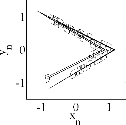
(a) (b)
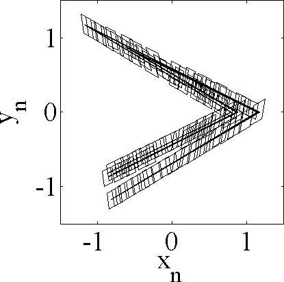
(c)

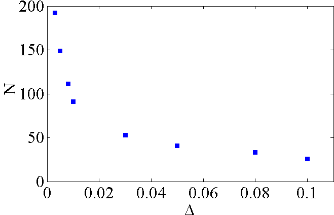
Figure 1: Building the partition for the Lozi attractor, for an isotropic constant diffusion tensor $\delta_{ij}\Delta$. In frames (a) and (b) $\Delta=0.01$. The deterministic attractor is the fractal structure in the background of each picture. Stochastic neighborhoods of a set of periodic points are indicated by their standard deviation parallelograms. (a) An initial partition: with only periodic points of periods $\leq 5$ much of the attractor remains to be covered. (b) The final, optimal partition covers the whole attractor, with no pair of neighborhoods overlapping by more than 50%. (c) $N$, the number of neighborhoods needed to achieve the optimal partition for a given noise strength $\Delta$.

The main utility of a good partition is that it provides a basis for an accurate and efficient estimate of long-time averages of observables defined on the dynamical system, of the form (1). As explained in sect. I.3, our goal here is to determine the stationary distribution ${\rho}(x)$. For that purpose, we use as basis Gaussian ellipsoids that satisfy the local stationarity condition (7) in each neighborhood of the optimal partition. A set of Gaussians centered at every point in the state space ${\cal M}$ forms an overcomplete, non-orthogonal basis for functions in $L^{2}({\cal M})$, as is well known from the study of coherent states of quantum harmonic oscillators Gottfried and Yan (2003). Our (also overcomplete and non-orthogonal) set of Gaussians is centered only on periodic points, which are dense in the deterministic attractor, but not in the entire state space. Therefore our basis is designed to resolve the structure of any function with support on the hyperbolic ‘strange set’ (an attractor or a repeller). The Gaussians are constructed so that their widths balance the noise spreading and the (time-forward or -backward) contraction of the deterministic dynamics. In the transverse directions, the basis gives the width of the global stationary distribution, locally everywhere determined by the balance between noise and dynamics. Along the attractor, the basis determines the minimum number of neighborhoods needed to fully resolve the structure of the stationary distribution.

There are numerical methods (such as refinements of Ulam’s method Ermann and Shepelyansky (2012)) that identify the asymptotic attractor by running long noisy trajectories, dropping the transients, and covering the attractor so revealed by a finite number of boxes. These algorithms have no a priori information about how the stationary distribution behaves transversely to the deterministic attractor, and they may easily overestimate the number of basis elements needed to resolve this structure. In contrast, in our approach the transverse structure is automatically accounted for by the local balance between the noise and the deterministic contraction along the stable, transverse directions, given by covariance matrix block $\hat{Q}_{cc}$ in (12). Furthermore, estimating ${\rho}(x)$ by binning long noisy trajectory over a finite number of attractor-covering boxes is feasible only in a low-dimensional state space, while (12) can be computed for state space of any dimension.

In discrete time dynamics, the stationary distribution is the ground-state eigenfunction of the Fokker-Planck evolution operator (2) with escape rate $\gamma$,

$${\cal L}\,{\rho}(x)=e^{-\gamma}{\rho}(x)\,.$$ (14)

In order to estimate the stationary distribution, we write it as a sum over the neighborhoods of the periodic points:

$${\rho}(x)=\sum\limits_{a=1}^{N}h_{a}\,\phi_{a}(x),$$ (15)

where $\phi_{a}=e^{-{x}{}^{\top}_{a}Q_{a}x_{a}}$ are the Gaussian basis functions, with $Q_{a}$ given by (12), and the coefficients $\{h_{a}\}$ to be determined. The truncation of the expansion (15) to $N$ basis functions follow from our optimal partition. We estimate the coefficients $h_{a}$ by minimizing the cost function

$$\int\left(\sum\limits_{a=1}^{N}h_{a}({\cal L}-e^{-\gamma})\phi_{a}(x)\right)^{2}dx,$$ (16)

together with the normalization constraint for ${\rho}(x)$. We can also estimate the escape rate of the system by minimizing the error with respect to $e^{-\gamma}$.

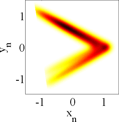
(a) (b)

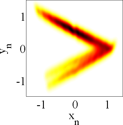
Figure 2: (Color online) The stationary distribution of the Lozi map with $\Delta=0.01$. (a) A direct numerical calculation obtained by running noisy trajectories for a long time. (b) The stationary distribution calculated with the optimal partition  method.

As an example, we apply the procedure to the Lozi map Lozi (1978)

$$x_{n+1} = 1-a|x_{n}|+b\ y_{n}$$

$$y_{n+1} = x_{n}$$ (17)

with parameters $a=1.85,b=0.3$ and isotropic, constant diffusion tensor $\delta_{ij}\Delta$ with $\Delta$ ranging in the interval $[0.003,0.1]$. Figure 1 (c), which shows the number $N$ of neighborhoods required by the optimal partition for a given $\Delta$, illustrates the efficiency of our method: $N$ goes from tens to few hundreds in the noise range considered. In order to test our algorithm, we also estimate ${\rho}(x)$ and $\gamma$ by a direct numerical simulation. The $(x,y)$ state space is divided into uniform mesh $6.4\times 10^{5}$ bins; we follow long stochastic trajectories and count how many times they visit each bin. The stationary distribution ${\rho}_{B}(x)$ is then the normalized frequency distribution of the whole grid. The deterministic Lozi map has a fixed point at the edge of attractor, whose stable manifold is the boundary of the deterministic basin of attraction. The noise makes it possible for a stochastic trajectory to cross this boundary and escape. We compute the escape rate as the ratio of the total number of points in the noisy trajectories to the number of escapes. Fig. 2 shows an example of the stationary distribution estimated with both methods, while in Fig. 3 we compare quantitatively the two procedures. In particular, we estimate the relative error between the stationary distribution ${\rho}$ computed with the optimal partition and ${\rho}_{B}$ computed on the uniform grid, by using a normalized $L^{2}$ distance, as

$$d({\rho},{\rho}_{B})=\frac{\int\left({\rho}(x)-{\rho}_{B}(x)\right)^{2}dx}{\int\left({\rho}_{B}(x)\right)^{2}dx}.$$ (18)

The two distributions are within $5\%$ of each other, whereas the escape rates differ by at most 10%, over a range of $\Delta$ that spans two orders of magnitude.

(a)
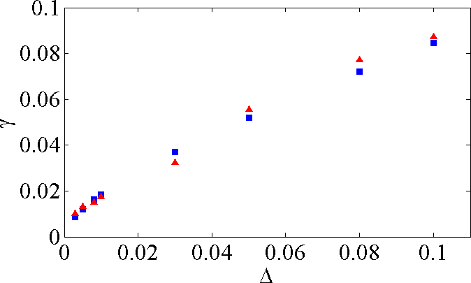
(b)

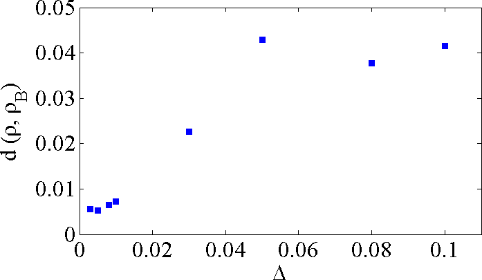
Figure 3: (a) The escape rate from the attractor as the function of the noise strength $\Delta$. Squares: uniform grid discretization method. Triangles: optimal partition. (b) The normalized $L^{2}$ distance $d({\rho},{\rho}_{B})$ between the corresponding stationary distributions.

IV Discussion

In conclusion, we have generalized the optimal partition hypothesis first formulated in Lippolis and Cvitanović (2010) to hyperbolic maps in arbitrary dimension, and tested the method on a two-dimensional system with weak white isotropic noise. As noise induces a finite resolution of the state space of any physical system, finite numbers of neighborhoods suffice to partition the state space explored by chaotic dynamics, and to estimate long-time averages of observables. Here we have used the deterministic unstable periodic orbits as the skeleton on which to build an optimal partition for the noisy state space. First we determine a local stationary distribution in the neighborhood of each periodic point by balancing the noise against the deterministic expansion or contraction. From the separation of expanding and contracting blocks in the covariance matrix that characterizes the Gaussian approximation to the local stationary distribution, we carve out a precise definition of neighborhood, the constituent of our partition, which is then used to approximate the global stationary distribution, estimate the escape rate (for open systems that allow escape), and any long-time averaged observable. Numerical tests confirm that the accuracy of our method is comparable to that of a uniform grid discretization, but the number neighborhoods required for our optimal partition ($\sim 10$ to 100) is three-four orders of magnitude smaller than the number of bins used in the uniform grid discretization method ($\sim 10^{5}$).

The problems dynamical chaos (or ‘turbulence’) theory faces nowadays are not two- but high-, even infinite-dimensional. Today it is possible to compute numerically exact periodic orbits (‘recurrent flows’ Cvitanović (2013)) in a variety of physically realistic turbulent fluid flows Nagata (1990); Gibson et al. (2008), but these calculations are at the limit of what current codes can do, and we hope that the methods presented here can provide sharp criteria for when a sufficient number of such solutions has been computed. Furthermore, unlike the uniform grid discretization, our partitions are smart, since they rely on the periodic orbits of the deterministic system as skeleton of the dynamics, as well as efficient, due to the finite (and optimal!) numbers of neighborhoods and corresponding basis functions. This, we believe, should make our algorithm less costly to implement than direct numerical simulations in higher dimensions, where discretizations would be impractical. With some modifications and application of Poincaré sections, the formalism can be applied to continuous time flows as well Gaspard (2002); Cvitanović and Lippolis (2012). Outstanding challenges include dealing with the lack of hyperbolicity in higher dimensions (marginal directions were treated in ref. Cvitanović and Lippolis (2012) for $1d$ maps), as well as extending the definition of neighborhood to other time-invariant sets, such as relative periodic orbits and partially hyperbolic invariant manifolds. Further technical issues, such as improving the efficiency of the minimization algorithm by modifying the basis of functions used in the computation of the stationary distribution, are also part of our agenda.