Quantum walks on simplicial complexes

Abstract

We construct a new type of quantum walks on simplicial complexes as a natural extension of the well-known Szegedy walk on graphs. One can numerically observe that our proposing quantum walks possess linear spreading and localization as in the case of the Grover walk on lattices. Moreover, our numerical simulation suggests that localization of our quantum walks reflect not only topological but also geometric structures. On the other hand, our proposing quantum walk contains an intrinsic problem concerning exhibition of nontrivial behavior, which is not seen in typical quantum walks such as Grover walks on graphs.

Keywords: quantum walk, simplicial complexes, tethered and movable quantum walks.

1 Introduction – Motivation and Aim –

The quantum walk is a quantum analogue of classical random walks [1]. Its primitive form of the discrete-time quantum walk on $\mathbb{Z}$ can be seen in Feynman’s checker board [2]. It is mathematically shown (e.g. [3]) that this quantum walk has a completely different limiting behavior from classical random walks, which is a typical example showing a difficulty of intuitive description of quantum walks’ behavior. By such an interesting observation and the efficiency of quantum walks in quantum search algorithms (see [4, 5] and their references), quantum walks are studied from various kinds of viewpoints such as the quantum information [6, 7, 8], approximation of physical process derived from the Dirac and Schrödinger equations [9, 10], experimental and industrial viewpoints [11, 12, 13, 14, 15], and so on.

A primitive form of the Grover walk on graphs has been appeared in [16]. This is considered as one of the most intensively-investigated quantum walks from the viewpoint of quantum information theory, a spectral graph theory [4, 17] and a scattering theory [17]. As a generalization of the Grover walk, the Szegedy walk is proposed to provide more abstractive discussions of applications such as quantum search algorithms [18]. Very recently, the Szegedy walk is applied to quantum PageRank algorithm on large complex networks [19, 20], for example. A key feature of the Szegedy walk is that the spectrum is decomposed into two parts : the inherited part associated with underlying random walks on graphs and the birth part with some multiplicities. In particular, the birth part reflects the cycle structure on graphs, and it induces localization of quantum walks, namely, the finding probability of quantum walks remains as a positive value even in the long time limit. These features are also discussed in [21] in the case of the Grover walk on crystal lattices.

The main aim of this paper is to construct a geometric multi-dimensional analogue of quantum walks on graphs. In earlier works, quantum walks on geometric objects embedded in multi-dimensional spaces are considered as ones on graphs. Such a traditional quantum walk can be regarded as transmission and reflection at vertices of one dimensional waves on edges of the graph. On the other hand, if we consider an analogue of quantum walks related to multi-dimensional waves, it is natural to consider quantum walks on geometric objects which admits multi-dimensional structures like planes or surfaces. Once one can construct such quantum walks, it is expected to study multi-dimensional feature of walks as well as their deeper geometric aspects.

In this paper we take simplicial complexes as a natural multi-dimensional extensions of graphs. The essence of the construction of quantum walks on simplicial complexes is to make an interaction of multi-dimensional waves satisfying the following postulates 1-3 in quantum mechanics [22];

1. Underlying space of dynamical system is a Hilbert space $\mathcal{H}$;

2. The time evolution is governed by a unitary operator on $\mathcal{H}$;

3. There exists a collection of orthogonal projections $\{E_{m}\}$ with $\sum_{m}E_{m}=I$ such that if the state $\psi\in\mathcal{H}$ is measured, then the probability that the result $m$ occurs is given by

   $$Prob(m)=\|E_{m}\psi\|_{\mathcal{H}}^{2}.$$

4. Moreover we provide the following additional postulate (cf. No-go lemma [23]):
   the time evolution can provide a non-trivial interaction, in particular, transmission and reflection of waves.

In this paper, we propose a notion of the non-trivial interaction as follows: we say non-trivial interaction exhibits if and only if the time evolution $U$ is neither tethered (Definition 2.14) nor non-interactive (Definition 2.15, cf. No-go lemma [23]).

For given $n$-dimensional simplicial complex $\mathcal{K}=\{K_{k}\}_{k=0}^{n}$, we propose the following walk which meets at least postulates 1–3 (see Definition 2.9 for details) and we check that the postulate 4 obviously holds for the simplicial complexes treated here by numerical simulations.

1. Total state space (postulate 1): We define a “directed” $n$-simplex by

   $$\tilde{K}_{n}=\{\pi[a_{0}a_{1}\cdots a_{n}]\mid|a_{0}a_{1}\cdots a_{n}|\in K_{n},\pi\in\mathcal{S}_{n+1}\}.$$

   The total state space is $\mathcal{H}=\ell^{2}(\tilde{K}_{n})$ with the standard inner product (see Definition 2.1 for the detailed setting of the simplicial complex).

2. Time evolution (postulates 2): Let $d_{0}^{(n)}:\ell^{2}(\tilde{K}_{n})\to\ell^{2}(\tilde{K}_{n-1})$ be a coisometric operator whose explicit expression is denoted by Definition 2.3, and also let $S:\ell^{2}(\tilde{K}_{n})\to\ell^{2}(\tilde{K}_{n})$ be a cyclic shift operator. Then the one-step time evolution operator is defined by

   $$U=S(2{d_{0}^{(n)}}^{*}d_{0}^{(n)}-I),$$

   where ${d_{0}^{(n)}}^{\ast}$ is the adjoint operator of $d_{0}^{(n)}$. This is a unitary operator on $\ell^{2}(\tilde{K}_{n})$ (Proposition 2.8). After one step unitary map $U$, an incident state in a simplex is changed to a linear combination of the states in the same simplex (reflection) and its adjacent simplices (transmission). See Figure 1.

3. Finding probability (postulate 3): We define the finding probability at a simplex $|\sigma|\in K_{n}$ with the initial state $\psi_{0}\in\ell^{2}(\tilde{K}_{n})$ after $m$-th iteration is

   $$\mu_{m}^{\psi_{0}}(|\sigma|)=\sum_{\pi\in\mathcal{S}_{n+1}}(U^{m}\psi_{0})(\pi\sigma)^{2}_{\tilde{K}_{n}}.$$

Remark that, when $n=1$, the original Szegedy walk on a graph [18, 21] is reconstructed. In that sense, this walk is a natural generalization of the Szegedy walk. In the above settings, we run this walk on several kinds of simplicial complexes by numerical simulations in this paper. Our numerical simulation results provide the following interesting observations.

Quantum walks on simplicial complexes reflect topology of simplicial complexes, as in the case of lattices discussed in [21]. Moreover, multi-dimensional geometric features yield richer aspects of our quantum walks. More precisely, we numerically obtain the following observations:

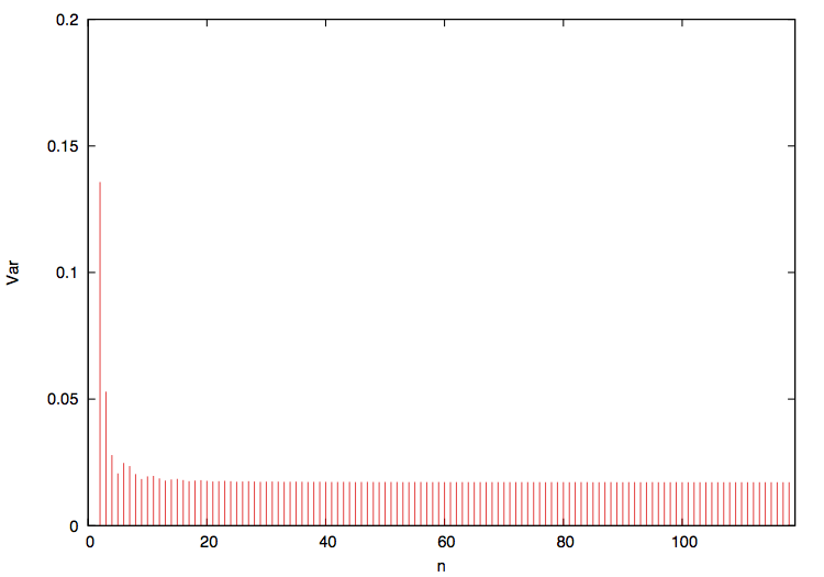
(a)

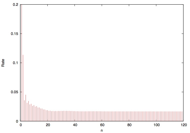
(b)

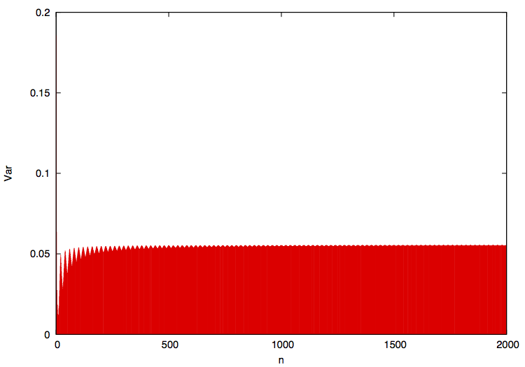
(c)

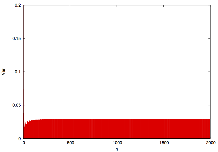
(d)

Figure 11: The graph of variance $V_{n}/n^{2}$ in (3.6): asymptotic behavior of the second moment of $\Psi_{n}/n$ with respect to the S-quantum walks $\Psi_{n}$. Row: time step $n$. Column: the value of $V_{n}/n^{2}$.

• Our quantum walks admit linear spreading and localizations, which are similar behaviors to traditional quantum walks on graphs (Figures 11 and 15).

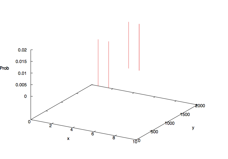
(a)

(b)

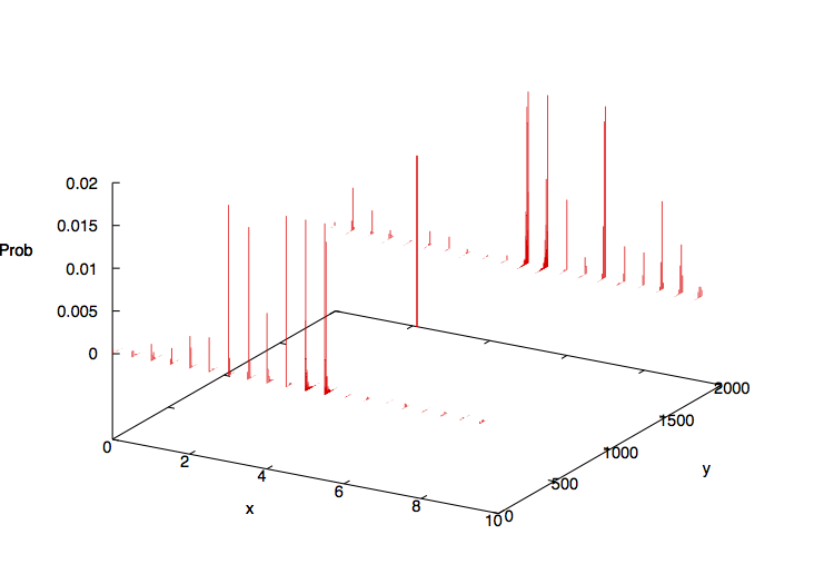
(c)

Figure 13: S-quantum walk on $\mathcal{K}_{1}$ : (a), (b), and on $\mathcal{K}_{2}$ : (c)

• Topological cycle structure brings about localization of quantum walks (Figures 13 and 15).

• Higher dimensional topological cycles such as cavities (Figure 7) can “absorb” localized states on cycles (Figures 7, 13 and 15).

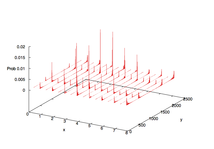
(a)

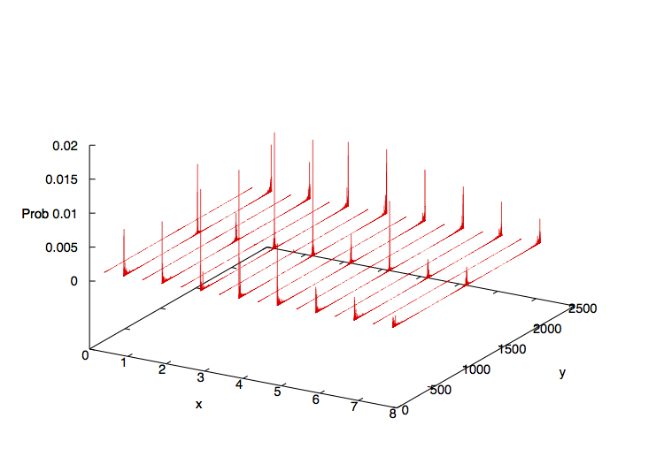
(b)

Figure 14: S-quantum walks on $\mathcal{K}_{3}$ : (a), versus on $\mathcal{K}_{1}$ : (b)

• Orientability of simplicial complexes also affects the behavior of quantum walks (Figures 14 and 15).

This paper is organized as follows. In Section 2, we construct a unitary operator on simplicial complexes which is a natural extension of quantum walks on graphs. In Section 3, we numerically study quantum walks constructed in Section 2. In particular, we study our quantum walks on the following geometric objects:

• $\mathbb{R}^{2}$: two dimensional Euclidian space corresponding to the simplicial complex $\mathcal{K}_{0}$;

• $S^{1}\times\mathbb{R}$: a infinite cylinder corresponding to the simplicial complex $\mathcal{K}_{1}$;

• an infinite cylinder with a tetrahedron with cavity corresponding to the simplicial complex $\mathcal{K}_{2}$;

• the Möbius band corresponding to the simplicial complex $\mathcal{K}_{3}$.

We observe the similar and different properties compared with the traditional quantum walks on graphs as stated in the above. Concrete implementations of our quantum walks and numerical simulation results are shown in Appendix.

2 Quantum walks on simplicial complexes

Let $\mathcal{K}$ be an $n$-dimensional simplicial complex and $K_{k}=K_{k}(\mathcal{K})$ be a collection of $k$-simplices which belongs to $\mathcal{K}$. Throughout this paper we consider the following class of simplicial complexes.

Definition 2.1.

We shall call an $n$-dimensional simplicial complex $\mathcal{K}=\{K_{k}\}_{k=0}^{n}$ admissible if the following conditions hold:

• $\mathcal{K}$ is strongly connected. See also Definition A.3;

• For each $k=0,\cdots,n-1$, every $|\tau|\in K_{k}$ is a primary face of some $|\sigma|\in K_{k+1}$. We do not assume that such a $(k+1)$-simplex $|\sigma|$ is uniquely determined. Moreover, assume that there is a positive integer $M$ such that

  $$\sharp\{|\sigma|\in K_{k+1}\mid|\sigma|\text{ admits }|\tau|\text{ as a face}\}\leq M<\infty$$

holds for all $|\tau|\in K_{k}$ and for each $k=0,\cdots,n-1$.

In this paper, we define the set of “directed” $k$-simplices $\tilde{K}_{k}\ (k=0,\cdots,n-1)$ associated with $K_{k}$ by the following, which is important to construct our quantum walks.

$$\tilde{K}_{k}:=\{\pi\sigma:=\pi[a_{0}a_{1}\cdots a_{k}]\mid|\sigma|=|a_{0}a_{1}\cdots a_{k}|\in K_{k},\ \pi\in\mathcal{S}_{k+1}\},$$

where $\mathcal{S}_{k+1}$ is the $(k+1)$-dimensional permutation group. For example, a $2$-simplex $|abc|\in K_{2}$ generates six different elements in $\tilde{K}_{2}$: $[abc]$, $[bca]$, $[cab]$, $[acb]$, $[cba]$ and $[bac]$. Whenever we use these notations, we distinguish $[abc]$ from $[bca]$, $[acb]$ and so on. On the other hand, we identify $|abc|$ with $|bca|$, $|abc|$, etc., which can be regarded as the support of directed simplices.

Now we define quantum walks on $\mathcal{K}$. Firstly, define a $\mathbb{C}$-linear space $\ell^{2}(\tilde{K}_{k})$ by

$$\ell^{2}(\tilde{K}_{k}):=\left\{f:\tilde{K}_{k}\to\mathbb{C}\mid\|f\|_{\tilde{K}_{k}}<\infty\right\}.$$

Here the inner product is given by the standard inner product, that is,

$$\langle f,g\rangle_{\tilde{K}_{k}}:=\sum_{\sigma\in\tilde{K}_{k}}\overline{f(\sigma)}g(\sigma).$$

Let $\|\cdot\|_{\tilde{K}_{k}}$ be the associated norm, namely, $\|f\|_{\tilde{K}_{k}}:=\langle f,f\rangle_{\tilde{K}_{k}}^{1/2}$. We take

$$\delta^{(k)}_{\sigma}(\sigma^{\prime}):=\begin{cases}1&\text{ if $\sigma^{\prime}=\sigma$}\\ 0&\text{ if $\sigma^{\prime}\not=\sigma$}\end{cases}$$

as the standard basis of $\ell^{2}(\tilde{K}_{k})$. One knows that the $\mathbb{C}$-linear space $\ell^{2}(\tilde{K}_{k})$ associated with the inner product $\langle\cdot,\cdot\rangle_{\tilde{K}_{k}}$ is a Hilbert space.

Fix a permutation on $(n+1)$-words $\pi\in\mathcal{S}_{n+1}$ whose order is $n+1$. That is,

$$\pi^{1}\not=\pi^{2}\not=\cdots\not=\pi^{n+1}=I.$$

As an example, we choose

$$\pi[a_{0}a_{1}\cdots a_{n-1}a_{n}]=[a_{1}a_{2}\cdots a_{n}a_{0}].$$ (2.1)

Throughout this paper, we only consider the permutation (2.1) for simplicity. We associate this permutation with the $n$-th total state space $\ell^{2}(\tilde{K}_{n})$ by

$$S_{\pi}\delta^{(n)}_{\sigma}:=\delta^{(n)}_{\pi\sigma},\quad\sigma\in\tilde{K}_{n}.$$

Definition 2.2 (Total state space).

We shall say the Hilbert space $(\ell^{2}(\tilde{K}_{n}),\langle\cdot,\cdot\rangle_{\tilde{K}_{n}})$ the total state space of the simplicial quantum walk on $\mathcal{K}$ defined below, where $n=\dim\mathcal{K}$.

Secondly, define a linear operator on the total state space and its adjoint operator.

Definition 2.3.

Let $i\in\{0,1,\cdots,n\}$. Define a map $\tilde{d}^{(n)}_{i}:\tilde{K}_{n}\to\tilde{K}_{n-1}$ by the following:

$$\tilde{d}^{(n)}_{i}[a_{0}a_{1}\cdots a_{n}]:=[a_{i+1}a_{i+2}\cdots a_{n}a_{0}a_{1}\cdots a_{i-1}].$$

Also, define $d^{(n)}_{i}:\ell^{2}({\tilde{K}_{n}})\to\ell^{2}({\tilde{K}_{n-1}})$ by the $\mathbb{C}$-linear extension of the following expression:

$$d^{(n)}_{i}\delta^{(n)}_{\sigma}=\overline{w(\pi^{i}\sigma)}\delta_{\tilde{d}^{(n)}_{i}\sigma}^{(n-1)},$$

where $w(\sigma)\in\mathbb{C}$ is a constant depending on $\sigma\in\tilde{K}_{n}$, and $\overline{w}$ is the complex conjugate of $w\in\mathbb{C}$.

For example, consider the case where $n=2$ and $\sigma=[abc]$. We then have

$$\tilde{d}^{(2)}_{0}([abc])=[bc],\quad\tilde{d}^{(2)}_{1}([abc])=[ca],\quad\tilde{d}^{(2)}_{2}([abc])=[ab],$$

which yield

$$d^{(2)}_{0}\delta^{(2)}_{[abc]}=\overline{w([abc])}\delta^{(1)}_{[bc]},\quad d^{(2)}_{1}\delta^{(2)}_{[abc]}=\overline{w([bca])}\delta^{(1)}_{[ca]},\quad d^{(2)}_{0}\delta^{(2)}_{[abc]}=\overline{w([cab])}\delta^{(1)}_{[ab]}.$$

One easily sees that $d^{(n)}_{i}=d^{(n)}_{0}\circ S_{\pi}^{j}$ holds for $i=0,\cdots,n$.

Definition 2.4.

Define a linear operator ${d^{(n)}_{i}}^{\ast}:\ell^{2}(\tilde{K}_{n-1})\to\ell^{2}(\tilde{K}_{n})$ by the $\mathbb{C}$-linear extension of the following formulation:

$${d^{(n)}_{i}}^{\ast}\delta_{\tau}^{(n-1)}:=\sum_{\sigma:\tilde{d}^{(n)}_{i}\sigma=\tau}w(\pi^{i}\sigma)\delta_{\sigma}^{(n)}.$$

Remark 2.5.

Easy calculations yield

$$S_{\pi}{d^{(n)}_{1}}^{\ast}={d^{(n)}_{0}}^{\ast},\quad S_{\pi}{d^{(n)}_{2}}^{\ast}={d^{(n)}_{1}}^{\ast},\quad\cdots,\quad S_{\pi}{d^{(n)}_{n}}^{\ast}={d^{(n)}_{n-1}}^{\ast},\quad S_{\pi}{d^{(n)}_{0}}^{\ast}={d^{(n)}_{n}}^{\ast},$$

since the unitary transpose $S_{\pi}^{\ast}$ of $S_{\pi}$ coincides with $S_{\pi}^{-1}$.

The linear operator ${d^{(n)}_{i}}^{\ast}$ is indeed the adjoint operator of $d^{(n)}_{i}$ in the following sense.

Lemma 2.6.

Assume that the function $w:\tilde{K}_{n}\to\mathbb{C}$ in the definition of $d_{i}$ is bounded. Then, for each $i=0,\cdots,n$, the following equality holds:

$$\langle d^{(n)}_{i}\psi,\phi\rangle_{\tilde{K}_{n-1}}=\langle\psi,{d^{(n)}_{i}}^{\ast}\phi\rangle_{\tilde{K}_{n}},\quad\forall\psi\in\ell^{2}(\tilde{K}_{n}),\ \phi\in\ell^{2}(\tilde{K}_{n-1}).$$

Proof.

Let $\psi=\sum_{\sigma\in\tilde{K}_{n}}\psi_{\sigma}\delta_{\sigma}^{(n)}\in\ell^{2}(\tilde{K}_{n})$ and $\phi=\sum_{\tau\in\tilde{K}_{n-1}}\phi_{\tau}\delta_{\tau}^{(n-1)}\in\ell^{2}(\tilde{K}_{n-1})$, where $\psi_{\sigma},\ \phi_{\tau}\in\mathbb{C}$. Direct computations yield

$$\langle\psi,{d^{(n)}_{i}}^{\ast}\phi\rangle_{\tilde{K}_{n}} =\sum_{\sigma\in\tilde{K}_{n}}\overline{\psi(\sigma)}({d^{(n)}_{i}}^{\ast}\phi)(\sigma)$$

$$=\sum_{\sigma\in\tilde{K}_{n}}\overline{\psi(\sigma)}\left(\sum_{\tau\in\tilde{K}_{n-1}}\phi_{\tau}({d^{(n)}_{i}}^{\ast}\delta_{\tau}^{(n-1)})(\sigma)\right)$$

$$=\sum_{\sigma\in\tilde{K}_{n}}\overline{\psi(\sigma)}\left(\sum_{\tau\in\tilde{K}_{n-1}}\phi_{\tau}\left(\sum_{\sigma^{\prime}\in\tilde{K}_{n}:\tilde{d}^{(n)}_{i}{\sigma^{\prime}}=\tau}w(\pi^{i}\sigma^{\prime})\delta_{\sigma^{\prime}}^{(n)}(\sigma)\right)\right)$$

$$=\sum_{\sigma\in\tilde{K}_{n}}\overline{\psi(\sigma)}\left(\phi_{\tilde{d}^{(n)}_{i}\sigma}w^{(n)}(\pi^{i}\sigma)\delta_{\sigma}^{(n)}(\sigma)\right)$$

$$=\sum_{\sigma\in\tilde{K}_{n}}\overline{\psi_{\sigma}}w(\pi^{i}\sigma)\phi_{\tilde{d}^{(n)}_{i}\sigma}.$$

Similarly,

$$\langle d^{(n)}_{i}\psi,\phi\rangle_{\tilde{K}_{n-1}} =\sum_{\tau\in\tilde{K}_{n-1}}\left(\sum_{\sigma\in\tilde{K}_{n}}w(\pi^{i}\sigma)\overline{\psi_{\sigma}}\delta_{\tilde{d}^{(n)}_{i}\sigma}^{(n-1)}(\tau)\right)\left(\sum_{\tau^{\prime}\in\tilde{K}_{n-1}}\phi_{\tau^{\prime}}\delta_{\tau^{\prime}}^{(n-1)}(\tau)\right)$$

$$=\sum_{\tau\in\tilde{K}_{n-1}}\left(\sum_{\sigma\in\tilde{K}_{n}}w(\pi^{i}\sigma)\overline{\psi_{\sigma}}\delta_{\tilde{d}^{(n)}_{i}\sigma}^{(n-1)}(\tau)\right)\phi_{\tau}.$$

Now the summand $\sum_{\sigma\in\tilde{K}_{n}}w(\pi^{i}\sigma)\overline{\psi_{\sigma}}\delta_{\tilde{d}^{(n)}_{i}\sigma}^{(n-1)}(\tau)$ is actually $\sum_{\sigma:\tilde{d}_{i}^{(n)}\sigma=\tau}w(\sigma)\overline{\psi_{\sigma}}$, which is a finite sum since $\mathcal{K}$ is admissible. Since each $|\tau|\in K_{n-1}$ has a coface $|\sigma|\in K_{n}$, then the sum $\sum_{\tau\in\tilde{K}_{n-1}}\sum_{\sigma:\tilde{d}_{i}^{(n)}\sigma=\tau}$ is exactly the same as $\sum_{\sigma\in\tilde{K}_{n}}$. Therefore

$$\langle d^{(n)}_{i}\psi,\phi\rangle_{\tilde{K}_{n-1}} =\sum_{\sigma\in\tilde{K}_{n}}\overline{\psi_{\sigma}}w(\pi^{i}\sigma)\phi_{\tilde{d}^{(n)}_{i}\sigma}.$$

Finally, calculations in both $\langle\psi,{d^{(n)}_{i}}^{\ast}\phi\rangle_{\tilde{K}_{n}}$ and $\langle d^{(n)}_{i}\psi,\phi\rangle_{\tilde{K}_{n-1}}$ make sense since $w$ is bounded. As a result, the proof is completed. ∎

Definition 2.7.

We shall say the function $w:\tilde{K}_{n}\to\mathbb{C}$ a weight on $\mathcal{K}$ if $w(\sigma)\not=0$ for all $\sigma\in\tilde{K}_{n}$ and

$$\sum_{\sigma\in\tilde{K}_{n}:\tilde{d}^{(n)}_{0}\sigma=\tau}|w(\pi^{i}\sigma)|^{2}=1$$

holds for all $\tau\in\tilde{K}_{n-1}$.

The second statement of the weight is equivalent to

$$\sum_{\sigma\in\tilde{K}_{n}:\tilde{d}^{(n)}_{i}\sigma=\tau}|w(\sigma)|^{2}=1,\quad\forall\tau\in\tilde{K}_{n-1},\quad i=0,\cdots,n.$$

By the definition, a weight $w$ on an admissible simplicial complex $\mathcal{K}$ satisfies the assumption of Lemma 2.6. Using the notion of weights, we obtain the following proposition, which is the center for constructing our quantum walk.

Proposition 2.8.

Let $\mathcal{K}$ be an admissible $n$-dimensional simplicial complex which admits a weight $w$. Then, for $i=0,\cdots,n$, the linear operator $C_{i}:=2{d^{(n)}_{i}}^{\ast}d^{(n)}_{i}-I$ is a unitary operator on $\ell^{2}(\tilde{K}_{n})$.

Proof.

Admissibility of $\mathcal{K}$ and the existence of a weight $w$ yield that both $d_{i}^{(n)}$ and ${d_{i}^{(n)}}^{\ast}$ are bounded and linear. Since $C_{i}^{\ast}=(2{d^{(n)}_{i}}^{\ast}d^{(n)}_{i}-I)^{\ast}=C_{i}$, it is sufficient to prove $C_{i}^{2}=I$. One knows

$$C_{i}^{2} =(2{d^{(n)}_{i}}^{\ast}d^{(n)}_{i}-I)^{2}=4{d^{(n)}_{i}}^{\ast}(d^{(n)}_{i}{d^{(n)}_{i}}^{\ast}-I)d^{(n)}_{i}+I.$$

Now we consider the linear operator $d_{i}d_{i}^{\ast}$. By the definition, we obtain

$$d^{(n)}_{i}{d^{(n)}_{i}}^{\ast}\delta_{\tau}^{(n-1)} =d^{(n)}_{i}\left(\sum_{\sigma\in\tilde{K}_{n}:\tilde{d}^{(n)}_{i}\sigma=\tau}w(\pi^{i}\sigma)\delta_{\sigma}^{(n)}\right)$$

$$=\sum_{\sigma\in\tilde{K}_{n}:\tilde{d}^{(n)}_{i}\sigma=\tau}\overline{w(\pi^{i}\sigma)}\cdot w(\pi^{i}\sigma)\delta_{\tilde{d}^{(n)}_{i}\sigma}^{(n-1)}.$$

The function $\delta_{\tilde{d}^{(n)}_{i}\sigma}^{(n-1)}$ in the sum of the right-hand side is equal to $\delta_{\tau}^{(n-1)}$. Since $w$ is a weight on $\mathcal{K}$, then we obtain

$$\sum_{\sigma\in\tilde{K}_{n}:\tilde{d}_{i}\sigma=\tau}\overline{w(\pi^{i}\sigma)}\cdot w(\pi^{i}\sigma)\delta_{\tau}^{(n-1)}=\delta_{\tau}^{(n-1)}.$$

Consequently, $d^{(n)}_{i}{d^{(n)}_{i}}^{\ast}\delta_{\tau}^{(n-1)}=\delta_{\tau}^{(n-1)}$ holds. Since $\tau\in\tilde{K}_{n-1}$ is arbitrary, then $d^{(n)}_{i}{d^{(n)}_{i}}^{\ast}=I$ holds. The equality $C_{i}^{2}=I$ thus holds and the proof is completed. ∎

Definition 2.9 (Simplicial quantum walks).

Let $\mathcal{K}$ be an admissible $n$-dimensional simplicial complex which admits a weight $w$. We shall say $C_{i}$ defined in Proposition 2.8 a (local) quantum coin on $\mathcal{K}$ and an operator $S_{\pi}$ a shift operator associated with a permutation $\pi\in\mathcal{S}_{n+1}$. An element $f\in\ell^{2}(\tilde{K}_{n})$ with $\|f\|_{\tilde{K}_{n}}=1$ is called a state. For the unitary operator $U:=S_{\pi}C_{0}$ and a state $f\in\ell^{2}(\tilde{K}_{n})$, define the (finding) probability at time $m$ at $|\sigma|\in K_{n}$ with the initial state $f$ by

$$\mu_{m}^{(f)}(|\sigma|):=\sum_{\tau:|\tau|=|\sigma|}\|U^{m}f(\tau)\|_{\tilde{K}_{n}}^{2}.$$

Finally, we call the triple $(U,\ell^{2}(\tilde{K}_{n}),\{\mu_{m}\}_{m\geq 0})$, or simply $U$, the simplicial quantum walk, or S-quantum walk for short, on $\mathcal{K}$.

Consider, as an example, the case $n=2$. The S-quantum walk $U$ scatters a state on a $2$-simplex $|\sigma|$ to the linear combination of a rotating state on the same $2$-simplex $|\sigma|$ and transmitted states to simplices adjacent to $|\sigma|$. The resulting state can be considered as the collection of the reflection (the former) and the transmission (the latter) of two dimensional waves. The illustration of the S-quantum walk on $\mathcal{K}$ is shown in Figure 1. It is a generalization of phenomena in quantum walks on graphs, as shown in Figure 2.

Note that $\sum_{|\sigma|\in K_{n}}\mu_{m}^{(f)}(|\sigma|)=1$ always holds for any state $f$ and all $m$, since $\|f\|_{\tilde{K}_{n}}=1$ and $U$ is unitary.

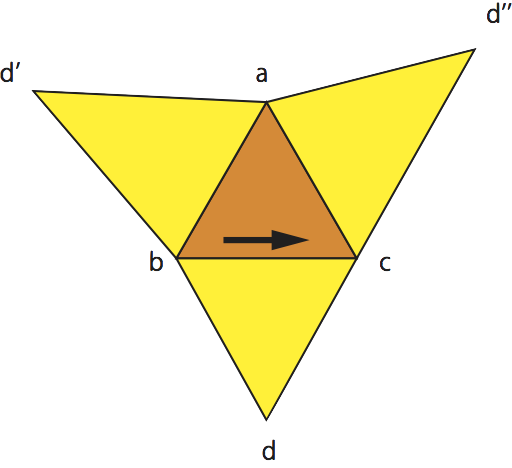
(a)

(b)

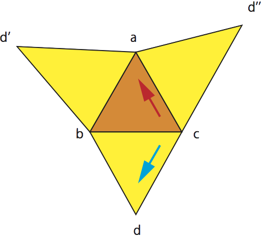
(c)

Figure 1: S-quantum walk $U$.

(a). The initial state $\delta^{(2)}_{[abc]}$.

(b). The quantum coin $C_{0}$. This figure shows the state $C_{0}\delta^{(2)}_{[abc]}=(2|w([abc])|^{2}-1)\delta^{(2)}_{[abc]}+2\overline{w([abc])}w([dbc])\delta^{(2)}_{[dbc]}$.

(c). The S-quantum walk $U=S_{\pi}C_{0}$. This figure shows the state $U\delta^{(2)}_{[abc]}=(2|w([abc])|^{2}-1)\delta^{(2)}_{[bca]}+2\overline{w([abc])}w([dbc])\delta^{(2)}_{[bcd]}$. The state on $|\sigma|=|abc|$ drawn by the red arrow represents the “reflection” of the state on $|\sigma|$. Similarly, the state on $|bcd|$ drawn by the blue arrow represents the “transmission” of the state on $|\sigma|$ to $|bcd|$.

(a)

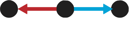
(b)

Figure 2: Quantum walk on graph.

(a). Initial state of $1$-dimensional quantum walk on an edge.

(b). Behavior of quantum walk on graph. Initial state (a) is mapped to the state via reflection (red) and transmission (blue). S-quantum walk on $\mathcal{K}$ described in Figure 1 can be considered as the multi-dimensional generalization of this behavior.

Remark 2.10.

Even if $\tau\in K_{n-1}$ is an $(n-1)$-simplex whose coface is only one $n$-simplex $\sigma$ and $\tilde{d}_{i}\sigma=\tau$, the identification of $C_{i}\delta_{\sigma}^{(n)}=\delta_{\sigma}^{(n)}$ also makes sense. In this case, we can interpret that the S-quantum walk $U$ only represents the reflection of waves without transmission.

Remark 2.11.

If $n=1$, the S-quantum walk on $\mathcal{K}$ is nothing but the Szegedy walk [18]. Moreover, if we assume that $w(e)=1/\sqrt{\deg(\tilde{d}_{1}^{(1)}e)}$ for all $e\in\tilde{K}_{1}$, then the corresponding S-quantum walk on $\mathcal{K}$ becomes the Grover walk on the graph $\mathcal{K}$.

Remark 2.12.

For a given $n$-dimensional admissible simplicial complex $\mathcal{K}$, we can define $d^{(k)}_{i}$ and ${d^{(k)}_{i}}^{\ast}$ in the same manner for the $k$-dimensional skeleton $\mathcal{K}^{(k)}=\{K_{j}\}_{j=0}^{k}$ of $\mathcal{K}$ for each $k=0,\cdots,n-1$.

We go back to construction of simplicial quantum walks. One can consider a permutation $\pi\in\mathcal{S}_{n+1}$ whose order is less than $n+1$ to define S-quantum walks. In this case, however, quantum walks can be trivial in the following sense.

Example 2.13.

Let $n=2$ and $\mathcal{K}$ be the simplicial complex drawn in Figure 1. Also, let $\pi^{\prime}\in\mathcal{S}_{3}$ be

$$\pi^{\prime}[abc]=[acb].$$

This permutation $\pi^{\prime}$ defines an S-quantum walk $U^{\prime}$ on $\mathcal{K}$ with a weight $w$. Consider time evolution of the state $\delta_{[abc]}^{(2)}$ under $U^{\prime}$. One easily knows that the state $\delta_{[abc]}$ does not transmit states on $|abd^{\prime}|$ and $|abd^{\prime\prime}|$ for arbitrary weights. In other words, states interact only between $|abc|$ and $|dbc|$ and we can observe no motions on quantum walks.

This example gives us the following problem : which permutation $\pi\in\mathcal{S}_{n+1}$ associates S-quantum walk exhibiting nontrivial behavior? We propose the following concept to formulate this problems mathematically.

Definition 2.14 (Tethered quantum walks).

For $\sigma=[a_{0}a_{1}\cdots a_{n}]\in\tilde{K}_{n}$, let $\{\sigma\}:=\{a_{0},a_{1},\cdots,a_{n}\}$. We say that a permutation $\pi\in\mathcal{S}_{n+1}$ induces tethered (S-)quantum walks on $\mathcal{K}$ if the following statement holds: for arbitrary weights on $\mathcal{K}$ and associated quantum walks $U=S_{\pi}C_{0}$, there exists a vertex $a_{j}\in\{\sigma\}$ such that the following two statements are equivalent for all $m\in\mathbb{N}$:

1. $\tau\in\tilde{K}_{n}$ satisfies $\langle\delta^{(n)}_{\tau},U^{m}\delta^{(n)}_{\sigma}\rangle_{\tilde{K}_{n}}\not=0$.

2. $a_{j}\in\{\tau\}$.

Conversely, we say that a permutation $\pi\in\mathcal{S}_{n+1}$ induces movable S-quantum walks on $\mathcal{K}$ if $\pi$ does not induce tethered quantum walks.

We easily know that the permutation $\pi^{\prime}:[abc]\mapsto[acb]$ induces tethered S-quantum walks on the complex in Example 2.13. In Example 2.13, $a_{j}$ in Definition 2.14 corresponds to vertices $\{b\}$ and $\{c\}$. The walk $U_{\pi^{\prime}}$ is always “tethered” around the starting position and never get far away from there. For these reasons, we apply $\pi\in\mathcal{S}_{3}$ given by (2.1) in the next section. By the definition of $U_{\pi}$, we expect that this $\pi$ induces movable quantum walks. As long as we observe numerical simulation results below, this permutation induces movable quantum walks. Our problem is then translated into determination of the class of permutations which induce movable quantum walks. On the other hand, a movable quantum walk does not always ensure a nontrivial behavior; we have to check if the quantum walk generates both transmission and reflection simultaneously. This is one of the other classification problems of quantum walks.

Definition 2.15 (Non-interactive quantum walks).

A simplicial quantum walk $U$ on $\mathcal{K}$ is non-interactive if, for any $\sigma\in\tilde{K}_{n}$ and for all $n\in\mathbb{N}$, there is a unique element $\tau\in\tilde{K}_{n}$ such that $\langle\delta^{(n)}_{\tau},U^{m}\delta^{(n)}_{\sigma}\rangle_{\tilde{K}_{n}}\not=0$. Conversely, $U$ is interactive if $U$ is not non-interactive.

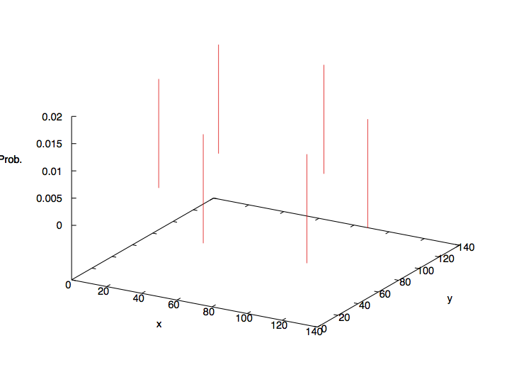
(a)

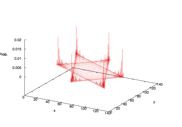
(b)

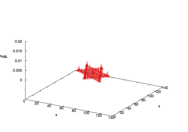
(c)

Figure 9: S-quantum walk on $\mathcal{K}_{0}$ with differential weights : The Hexagram

In general, interactive properties of quantum walks depend on their constructions, as indicated in the No-go lemma by Meyer [23]. This problem is also nontrivial in the construction of quantum walks on given simplicial complexes. In the case of S-quantum walks, weights determine whether or not quantum walks are interactive. In this paper, we have two examples of the non-interactive quantum walks which exhibit only the transmission without reflection. See Figs. 9-(a) and 13-(a). Our numerical simulations in the next section suggest that appropriate choice of weights let S-quantum walks interactive.

Both notions of tethered quantum walks and non-interactivity ask us a question of appropriate construction of quantum walks. In other words, these notions ask us whether we can choose an appropriate weight on a given complex $\mathcal{K}$ so that quantum walk $U$ on it is movable and interactive. Example 2.13 indicates that mobility of walks concerns with the choice of permutations, namely, shift operators. As indicated in the S-quantum walk on $\mathbb{R}^{2}$ with the weight (3.1) in the next section, which is a non-interactive quantum walk, the interactivity of walks concerns with the choice of coin operators.

3 Behavior of S-quantum walks – numerical study

In this section, we study how an S-quantum walk $U$ behaves on simplicial complexes. Throughout this section we only consider the case $n=2$. Our object here is to study relationships between geometry of $\mathcal{K}$ and nontrivial dynamics of $U$ such as localization. Here we study quantum walks on the following sample spaces:

Subsection 3.1 :

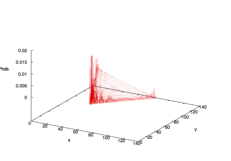
(a)

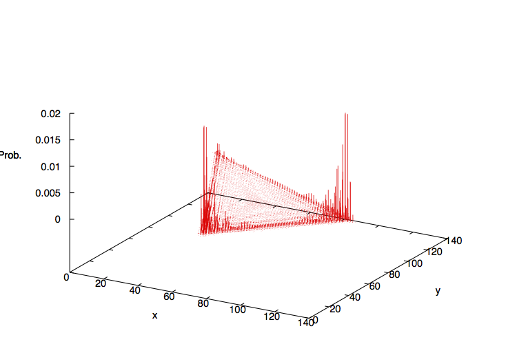
(b)

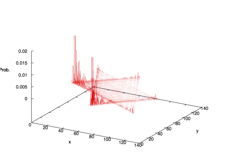
(c)

Figure 10: S-quantum walk on $\mathcal{K}_{0}$ with different initial states : The Triangle

$\mathbb{R}^{2}$. The corresponding simplicial complex is $\mathcal{K}_{0}$. Numerical results are shown in Figures 9 and 10.

Subsection 3.2 :

an infinite cylinder. The corresponding simplicial complex is $\mathcal{K}_{1}$. Numerical results are shown in Figures 13-(a), (b) and 14-(b).

Subsection 3.3 :

an infinite cylinder with a tetrahedron. The corresponding simplicial complex is $\mathcal{K}_{2}$. Numerical results are shown in Figure 13-(c).

Subsection 3.4 :

the Möbius band. The corresponding simplicial complex is $\mathcal{K}_{3}$. Numerical results are shown in Figure 14-(a).

3.1 S-quantum walk on $\mathbb{R}^{2}$

Here we consider one of the simplest examples, the quantum walk on $\mathbb{R}^{2}$.

3.1.1 Setting

First we represent $\mathbb{R}^{2}$ as a polyhedron via the simplicial decomposition. In the case of $\mathbb{R}^{2}$, one of the simplest decomposition is the uniform triangular decomposition drawn in Figure 3. We shall use such a decomposition as a sample examination. Let $\mathcal{K}_{0}$ be the obtained simplicial complex.

We shall derive the algorithmic procedure of the time evolution so that readers easily follow a series of computations. To implement the discrete-time evolution of S-quantum walk $U$, we take one-to-one correspondence between CONB on $\ell^{2}(\tilde{K}_{2})$ and its graphical representation shown in Figures 3 and 4. See also Remark 3.1 below.

Remark 3.1 (Notations in Case 1, 2 below and Appendix B).

We use the following notations for describing one time evolution of quantum walks. They let us construct time evolution of quantum walks on concrete simplicial complexes systematically.

Rule 1:

We label each simplex by integers. In the case of quantum walk on $\mathcal{K}_{0}$, for example, it is sufficient to consider $2N^{2}$ $2$-simplices for sufficiently large $N$. We then correspond each simplex to an integer from $0$ to $2N^{2}-1$, $\{2(iN+j)+k\mid i,j=0,\cdots,N-1,k=0,1\}$. In our notations, variable $i$ denotes the $x$-coordinate of indexed simplices and $j$ denotes the $y$-coordinate of indexed simplices. Furthermore, our complexes consist of two kinds of triangles, the lower one and the upper one (Figure 4). $k=0,1$ correspond to lower and upper triangles, respectively. We label the lower triangle $m$ and the upper triangle $m+1$, where $m\in\{2(iN+j)\mid i,j\in\mathbb{Z}\}$ if it is defined, unless otherwise noted.

Rule 2:

$\delta_{m,l}$ denotes the basis labeled by $m$ and $l$. Here $m$ is the index labeling $|\sigma|$ as an element of $K_{2}$, and $l\in\{0,1,\cdots,5\}$ denotes the index determined by the rule drawn in Figure 4. Similarly, we identify the weight $w(\sigma)$ for $\sigma\in\tilde{K}_{2}$ with $w_{m,l}$ in the same manner.

Rule 3:

In the case of quantum walks on cylinder, Subsections 3.2 and 3.3, we impose the periodic boundary conditions on boundaries. In our arguments, the periodic boundary condition in the $x$-coordinate is imposed. In the case of Möbius bands, we impose twisted identification in the $x$-coordinate. Details are shown in Subsection 3.4.

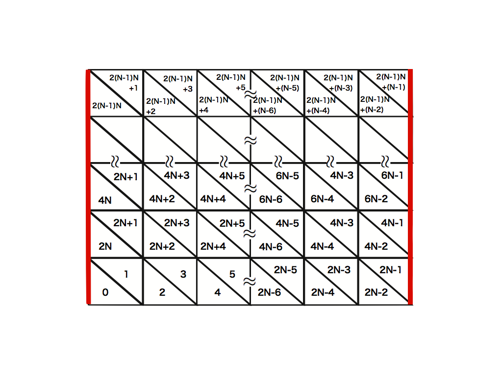
Figure 3: Uniform simplicial decomposition $\mathcal{K}_{0}$ of $\mathbb{R}^{2}$.

This decomposition can be realized by, say, dividing the unit square $[0,1]\times[0,1]$ into $2$ triangles. In practical computations we make such complex on $[-N,N]\times[-N,N]\subset\mathbb{R}^{2}$, consisting of $2N^{2}$ triangles. When we consider the S-quantum walk on an infinite cylinder (Subsection 3.2), we impose the periodic boundary condition on, say, two lines drawn by red lines.

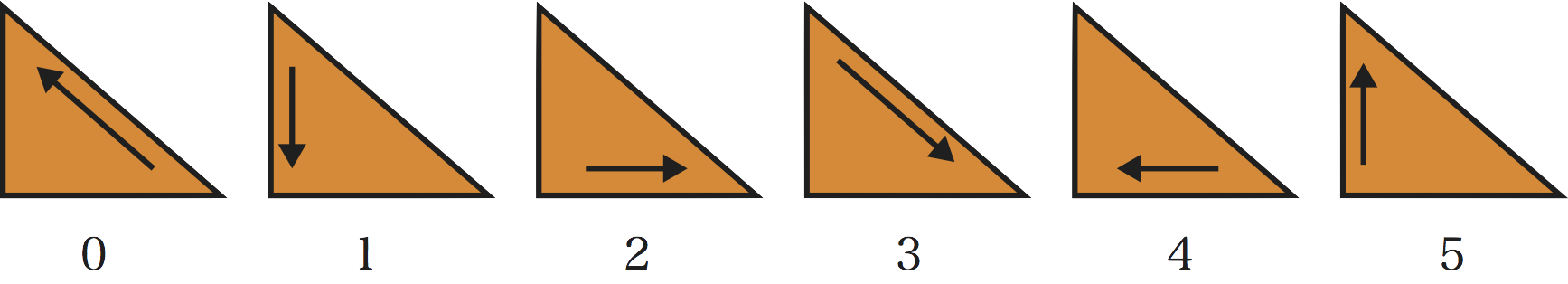
(a)

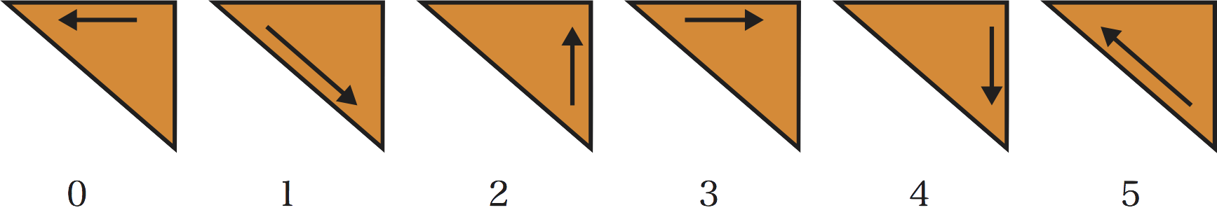
(b)

Figure 4: Labeling of bases.

(a): The graphical representation of basis $\delta_{2(iN+j),l}$, $l\in\{0,1,2,3,4,5\}$. (b): The graphical representation of basis $\delta_{2(iN+j)+1,l}$, $l\in\{0,1,2,3,4,5\}$.

Case 1: the lower triangle (Figure 4-(a))

By following the definition of $U$, the evolution of a state on a lower triangle is given by

$$\begin{pmatrix}\delta_{2(iN+j),0}\\ \delta_{2(iN+j),1}\\ \delta_{2(iN+j),2}\\ \delta_{2(iN+j),3}\\ \delta_{2(iN+j),4}\\ \delta_{2(iN+j),5}\end{pmatrix}$$

$$\mapsto\begin{pmatrix}(2|w_{2(iN+j),0}|^{2}-1)\cdot\delta_{2(iN+j),1}\\ (2|w_{2(iN+j),1}|^{2}-1)\cdot\delta_{2(iN+j),2}\\ (2|w_{2(iN+j),2}|^{2}-1)\cdot\delta_{2(iN+j),0}\\ (2|w_{2(iN+j),3}|^{2}-1)\cdot\delta_{2(iN+j),4}\\ (2|w_{2(iN+j),4}|^{2}-1)\cdot\delta_{2(iN+j),5}\\ (2|w_{2(iN+j),5}|^{2}-1)\cdot\delta_{2(iN+j),3}\end{pmatrix}+\begin{pmatrix}2\overline{w_{2(iN+j),0}}w_{2(iN+j)+1,5}\cdot\delta_{2(iN+j)+1,3}\\ 2\overline{w_{2(iN+j),1}}w_{2((i-1)N+j)+1,4}\cdot\delta_{2((i-1)N+j)+1,5}\\ 2\overline{w_{2(iN+j),2))}}w_{2(iN+(j-1))+1,3}\cdot\delta_{2(iN+(j-1))+1,4}\\ 2\overline{w_{2(iN+j),3}}w_{2(iN+j)+1,1}\cdot\delta_{2(iN+j)+1,2}\\ 2\overline{w_{2(iN+j),4}}w_{2(iN+(j-1))+1,0}\cdot\delta_{2(iN+(j-1))+1,1}\\ 2\overline{w_{2(iN+j),5}}w_{2((i-1)N+j)+1,2}\cdot\delta_{2((i-1)N+j)+1,0}\end{pmatrix}.$$

The first term of the right hand side represents the “reflection” of waves and the second represents the “transmission” of waves to the adjacent upper triangle.

Case 2: the upper triangle (Figure 4-(b))

Similarly, the evolution of the state on an upper triangle is given by

$$\begin{pmatrix}\delta_{2(iN+j)+1,0}\\ \delta_{2(iN+j)+1,1}\\ \delta_{2(iN+j)+1,2}\\ \delta_{2(iN+j)+1,3}\\ \delta_{2(iN+j)+1,4}\\ \delta_{2(iN+j)+1,5}\end{pmatrix}$$

$$\mapsto\begin{pmatrix}(2|w_{2(iN+j)+1,0}|^{2}-1)\cdot\delta_{2(iN+j)+1,1}\\ (2|w_{2(iN+j)+1,1}|^{2}-1)\cdot\delta_{2(iN+j)+1,2}\\ (2|w_{2(iN+j)+1,2}|^{2}-1)\cdot\delta_{2(iN+j)+1,0}\\ (2|w_{2(iN+j)+1,3}|^{2}-1)\cdot\delta_{2(iN+j)+1,4}\\ (2|w_{2(iN+j)+1,4}|^{2}-1)\cdot\delta_{2(iN+j)+1,5}\\ (2|w_{2(iN+j)+1,5}|^{2}-1)\cdot\delta_{2(iN+j)+1,3}\end{pmatrix}+\begin{pmatrix}2\overline{w_{2(iN+j)+1,0}}w_{2(iN+(j+1)),4}\cdot\delta_{2(iN+(j+1)),5}\\ 2\overline{w_{2(iN+j)+1,1}}w_{2(iN+j),3}\cdot\delta_{2(iN+j),4}\\ 2\overline{w_{2(iN+j)+1,2}}w_{2((i+1)N+j),5}\cdot\delta_{2((i+1)N+j),3}\\ 2\overline{w_{2(iN+j)+1,3)}}w_{2(iN+(j+1)),2}\cdot\delta_{2(iN+(j+1)),0}\\ 2\overline{w_{2(iN+j)+1,4}}w_{2((i+1)N+j),1}\cdot\delta_{2((i+1)N+j),2}\\ 2\overline{w_{2(iN+j)+1,5}}w_{2(iN+j),0}\cdot\delta_{2(iN+j),1}\end{pmatrix}.$$

As in the case of lower triangles, the first term of the right hand side represents the “reflection” of waves and the second represents the “transmission” of waves to the adjacent lower triangle.

All states evolve according to one of the above rules. We are then ready to compute S-quantum walk on $\mathbb{R}^{2}$.

3.1.2 S-quantum walk on $\mathbb{R}^{2}$

Let the triangle $|abc|\in K_{2}$ be located at the center of $N\times N$ lattice, in particular, $\delta^{(2)}_{\pi^{i}[abc]}=\delta_{\frac{N}{2}\times N+\frac{N}{2}+0,i}$. We set the initial state $\Psi_{0}=\sum_{i=0}^{2}\varphi_{\pi^{i}[abc]}\delta^{(2)}_{\pi^{i}[abc]}+\sum_{i=0}^{2}\varphi_{\pi^{i}[acb]}\delta^{(2)}_{\pi^{i}[acb]}\in\ell^{2}(\tilde{K}_{2})$, where

$$\varphi_{\pi^{i}[abc]}=\varphi_{\pi^{i}[acb]}=1/\sqrt{6},\quad i=0,1,2.$$

The S-quantum walk with the identical weight, namely,

$$w(\sigma)\equiv 1/\sqrt{2},\quad\forall\sigma\in\tilde{K}_{2},$$ (3.1)

is shown in Figure 9-(a).

Next, we change the weight into

$$w(\sigma_{1}) \equiv\sqrt{1/3}\quad\text{ for all $\sigma_{1}\in\tilde{K}_{2}$ with $|\sigma_{1}|$ being a lower triangle},$$

$$w(\sigma_{2}) \equiv\sqrt{2/3}\quad\text{ for all $\sigma_{2}\in\tilde{K}_{2}$ with $|\sigma_{2}|$ being an upper triangle}.$$ (3.2)

The computation result is drawn in 9-(b). Additionally, the quantum walk with the weight

$$w(\sigma_{1}) \equiv\sqrt{1/10}\quad\text{ for all $\sigma_{1}\in\tilde{K}_{2}$ with $|\sigma_{1}|$ being a lower triangle},$$

$$w(\sigma_{2}) \equiv\sqrt{9/10}\quad\text{ for all $\sigma_{2}\in\tilde{K}_{2}$ with $|\sigma_{2}|$ being an upper triangle}$$ (3.3)

is drawn in Figure 9-(c). In any cases, the state spreads in six-directions drawing a hexagram. In Figure 9-(a), no reflection occurs during time evolutions. These pictures imply that the ballistic spreading, which is the strongest spreading, is exhibited in S-quantum walks with uniform weights. Note that this is a similar behavior to the two-state Grover walk on $\mathbb{Z}$. This walk with the weight (3.1) is thus a non-interactive quantum walk. However, we can adjust the weight such as (3.2) and (3.3) to make the interactions. See Figs. 9-(b) and (c). These pictures also imply that, the bigger the difference between $w(\sigma_{1})$ and $w(\sigma_{2})$ is, the smaller the size of hexagram is. This observation is related to the pseudo velocity of the linear spreading.

Next we fix the weight $w$ by (3.2) and change the initial state into $\Psi_{0}=\delta^{(2)}_{[abc]}\in\ell^{2}(\tilde{K}_{2})$. Resulting behavior is shown in Figure 10. In this case, the state spreads drawing a triangle. Similarly, the quantum walk with the initial state $\Psi_{0}=\frac{1}{\sqrt{2}}\delta^{(2)}_{[abc]}+\frac{1}{\sqrt{2}}\delta^{(2)}_{[bca]}=\frac{1}{\sqrt{2}}\delta^{(2)}_{[abc]}+\frac{1}{\sqrt{2}}\delta^{(2)}_{\pi[abc]}\in\ell^{2}(\tilde{K}_{2})$ spreads linearly. Its support is also a similar triangle as shown in Figure 10-(b). On the other hand, if we consider the quantum walk with the initial state $\Psi_{0}=\frac{1}{\sqrt{2}}\delta^{(2)}_{[abc]}+\frac{1}{\sqrt{2}}\delta^{(2)}_{[acb]}\in\ell^{2}(\tilde{K}_{2})$, then the walk spreads drawing a hexagram like Figure 10-(c).

3.1.3 Comparison with quantum walk on the triangular lattice

We compare the behavior of the Grover walk on the triangular lattice with S-quantum walk on $\mathbb{R}^{2}$. The asymptotic behavior of the quantum walk on lattices, in particular, the Grover walk is studied not only numerically [24] but mathematically [21]. It is worth studying how the difference of dimension of complexes affect dynamics. Our criteria are focused on important and essential properties of quantum walks, localization and linear spreading.

Remark 3.2.

Here we review localization and linear spreading of quantum walks on a lattice $L$.

1. We say that localization occurs if there exists a point ${\bf x}\in L$ such that

   $$\limsup_{n\to\infty}\mu_{n}({\bf x})>0,$$

   where $\mu_{n}$ is the probability of the quantum walk $\Psi_{n}$ at time $n$ and position ${\bf x}\in L$ given by

   $$\mu_{n}({\bf x}):=\sum_{e\in\tilde{K}_{1}:o(e)={\bf x}}\|\Psi_{n}(e)\|^{2}_{\tilde{K}_{1}}.$$

   Here $o(e)$ is the origin vertex of the directed edge $e$. For example, if $e=ab$, then $o(e)=a$. Similarly, if $e=ba$, then $o(e)=b$. See [21] for details.

2. We say that linear spreading happens if

   $$\lim_{n\to\infty}\frac{V_{n}}{n^{2}}\in(0,\infty),$$ (3.4)

   where $V_{n}$ is the radial variance of the quantum walk $\Psi_{n}$ defined by

   $$V_{n}:=\left\{\sum_{x\in L}\|{\bf x}\|^{2}\mu_{n}({\bf x})^{2}-\left(\sum_{x\in L}\|{\bf x}\|\mu_{n}({\bf x})\right)^{2}\right\}$$ (3.5)

   and $\|{\bf x}\|$ is the Euclidean norm of ${\bf x}$.

The relationship (3.4) corresponds to weak convergence of the random variable $\Psi_{n}/n$. The denominator $n$ corresponds to the linearity of spreading rates, which is a quite different property from classical random walks.

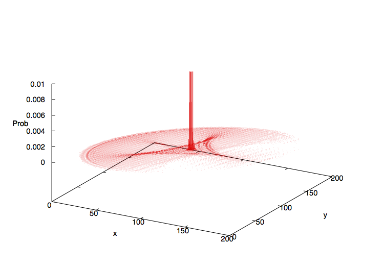
(a)

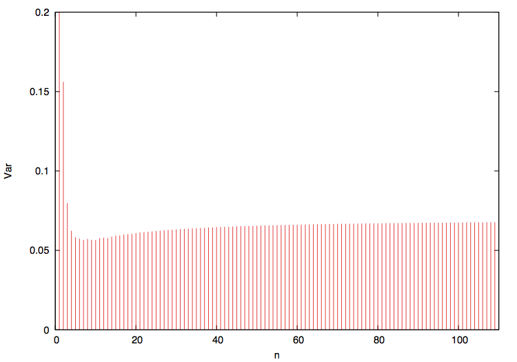
(b)

Figure 12: The Grover walk $\Psi_{n}$ on the triangular lattice

In [21], it is shown that the Grover walk on the triangular lattice exhibits both localization and linear spreading, as shown in Figure 12. On the contrast, we cannot observe localization in the case of S-quantum walks on $\mathcal{K}_{0}$, which can be seen in Figure 9 as noted before. This is a crucial difference between quantum walk on the triangular lattice and on $\mathcal{K}_{0}$. Such an observation can be stated more topologically. In [21], it is shown that the Grover walk on a finite graph $G$ exhibits localization if $G$ possesses a cycle in the homological sense. In other words, nontrivial first homology classes of $G$ induce localization. On the other hand, the simplicial complex $\mathcal{K}_{0}$ has no “cycles”, that is, topological holes such as rings and cavities. One can thus expect that the dimension and topology of simplicial complexes have great influences on the behavior of quantum walks.

Next, in order to study the spreading rate of $U$ on $\mathcal{K}_{0}$, we compute the radial variance

$$V_{n}=V_{n}^{(f)}:=\left\{\sum_{|\sigma|\in K_{2}}\sum_{{\bf x}=(x,y)\in|\sigma|}\|{\bf x}\|^{2}\mu_{n}^{(f)}(|\sigma|)^{2}-\left(\sum_{|\sigma|\in K_{2}}\sum_{{\bf x}=(x,y)\in|\sigma|}\|{\bf x}\|\mu_{n}^{(f)}(|\sigma|)\right)^{2}\right\},$$ (3.6)

corresponding to (3.5). Here $f$ denotes an initial state, but we often drop the letter $(f)$ if initial states are clear in the context. In practical computations, we condense the density and the probability $\mu_{n}$ of each simplex on a point, say, a vertex for simplicity. The time evolution of $V_{n}/n^{2}$ is drawn in Figure 11-(a). This figure shows that the quantity $V_{n}/n^{2}$ is close asymptotically to a certain positive value like (3.4), which implies that linear spreading happens for S-quantum walk on $\mathcal{K}_{0}$.

3.2 S-quantum walk on an infinite cylinder

Next we consider the S-quantum walk on an infinite cylinder $S^{1}\times\mathbb{R}$. Note that an infinite cylinder possesses a topological cycle, more precisely, the nontrivial first homology class (see Figure 6 in Appendix A for quick and intuitive understanding of homology). In the case of Szegedy walks on graphs, nontrivial cycle structure can induce localization [21]. Our focus in this section is to study if the nontrivial homology of simplicial complexes can induce localization. As in the case of $\mathbb{R}^{2}$, we derive a triangular decomposition of $S^{1}\times\mathbb{R}$ as the first step.

3.2.1 Setting

First we prepare a large rectangular domain with the uniform triangular decomposition. In this case we set $R\times N$-pairs of lower and upper triangles, where $R$ is a positive integer not so large, say, $10$ and $N$ is a large integer, say, $2000$. We additionally impose the periodic boundary condition on the $x$-axis. See Figure 3. The time evolution rule is the same as in the case of $\mathbb{R}^{2}$ with the additional periodic boundary condition. Let $\mathcal{K}_{1}$ be the obtained simplicial complex.

3.2.2 S-quantum walk on an infinite cylinder

We set the initial state $\Psi_{0}=\sum_{i=0}^{2}\varphi_{\pi^{i}[abc]}\delta^{(2)}_{\pi^{i}[abc]}+\sum_{i=0}^{2}\varphi_{\pi^{i}[acb]}\delta^{(2)}_{\pi^{i}[acb]}\in\ell^{2}(\tilde{K}_{2})$, where

$$\varphi_{\pi^{i}[abc]}=\varphi_{\pi^{i}[acb]}=1/\sqrt{6},\quad i=0,1,2.$$ (3.7)

The S-quantum walk with the identical weight, namely, $w(\sigma)\equiv 1/\sqrt{2}$ is shown in Figure 13-(a). Next, we change the weight into (3.2), namely,

$$w(\sigma_{1}) \equiv\sqrt{1/3}\quad\text{ for all $\sigma_{1}\in\tilde{K}_{2}$ with $|\sigma_{1}|$ being a lower triangle},$$

$$w(\sigma_{2}) \equiv\sqrt{2/3}\quad\text{ for all $\sigma_{2}\in\tilde{K}_{2}$ with $|\sigma_{2}|$ being an upper triangle}.$$

The computation result is depicted by Figure 13-(b). In both cases, we can observe a positive probability density on the central circle on which the initial state is located. These pictures indicate that localization occurs for $U$ on $S^{1}\times\mathbb{R}$. Now we compute the time-averaged probability of S-quantum walks with the initial state $f$ defined by

$$\bar{\mu}_{T}(|\sigma|)\equiv\bar{\mu}_{T}^{(f)}(|\sigma|):=\frac{1}{T}\sum_{m=0}^{T-1}\mu_{m}^{(f)}(|\sigma|),\quad|\sigma|\in K_{2}.$$ (3.8)

The calculation result is shown in Figure 15. The time-averaged probability $\bar{\mu}_{T}(|abc|)$ converges to a positive value as $T\to\infty$, which leads to the other suggestion that the localization occurs at the starting simplex $|abc|$.

As S-quantum walks on $\mathbb{R}^{2}$, time evolutions of the radial variance $V_{n}/n^{2}$ with different weights are shown in Figure 11-(c) and (d), where $V_{n}$ is given by (3.6). These figures show that the quantity $V_{n}/n^{2}$ converges to a certain positive value for quantum walks on $\mathcal{K}_{1}$. These observations imply that linear spreading happens on the S-quantum walk on $S^{1}\times\mathbb{R}$.

Remark 3.3.

In the case of $S^{1}\times\mathbb{R}$, there is a direction of the quantum walk such that a state stays in a compact subset of $S^{1}\times\mathbb{R}$, which reflects a bounded ring structure of the cylinder, that is, a generator of the nontrivial first homology group $H_{1}(S^{1}\times\mathbb{R};\mathbb{Z})\cong\mathbb{Z}$.

3.3 S-quantum walk on an infinite cylinder with a tetrahedron

In the third example, we consider the S-quantum walk on $\mathcal{K}_{2}$: an infinite cylinder discussed in the previous subsection with a tetrahedron. Tetrahedra have nontrivial cavities which generate the second homology classes. Here we consider the effect of such homology classes on S-quantum walks.

3.3.1 Setting

As in previous subsections, we construct a simplicial complex as the first step. We prepare the simplicial complex $\mathcal{K}_{1}$ and attach a tetrahedron somewhere on $\mathcal{K}_{1}$ to obtain the simplicial complex $\mathcal{K}_{2}$. The brief illustration of $\mathcal{K}_{2}$ around a tetrahedron is shown in Figure 7. The labeling of $2$-simplices are derived as in the case of $\mathcal{K}_{1}$ as well as the description in Figure 7. One can realize this construction in the standard manner and we omit the detail.

The additional algorithmic procedure of S-quantum walks on $\mathcal{K}_{2}$ is listed in Appendix B.

3.3.2 S-quantum walk on an infinite cylinder with a tetrahedron

We set the initial state $\Psi_{0}\in\ell^{2}(\tilde{K}_{2})$ by (3.7). Note that the $2$-simplex $|abc|$ is now set by a part of the tetrahedron in $\mathcal{K}_{2}$. See Figure 7. We then fix the weight

$$w(\sigma)\equiv 1/\sqrt{\deg(\tilde{d}_{0}^{(2)}\sigma)},\quad\text{ where }\deg(\tilde{d}_{0}^{(2)}\sigma):=\sharp\{\tau\in\tilde{K}_{1}:\tilde{d}_{0}^{(2)}\sigma=\tau,\sigma\in\tilde{K}_{2}\}.$$ (3.9)

In the case of quantum walks on graphs, such weight corresponds to the Grover walk on graphs.

The S-quantum walk with the weight (3.9) and the initial state $\Psi_{0}$ is shown in Figure 13-(c). In this example, localization cannot be observed around the central cycle comparing with the previous example on $\mathcal{K}_{1}$. Instead, we can see the localization on the “bump”, that is, the tetrahedron. Indeed, in the early stage the state with positive probability density on the circle is observable. After sufficient large time evolutions, such a state is absorbed by the tetrahedron. Such a phenomenon can be observed from time-averaged probability $\bar{\mu}_{T}$ given in (3.8). The measure $\bar{\mu}_{T}$ at the starting simplex $|abc|$ converges to a positive value as $T\to\infty$ as shown in Figure 15. On the other hand, the measure at a simplex off the tetrahedron but on the central cycle tends to zero, while the measure for S-quantum walk on $\mathcal{K}_{1}$ at the simplex on the central cycle tends to a positive value. Compare the graph “tetra-off” with “cylinder-transmit-adjacent” in Figure 15. These observations imply that the higher dimensional homology classes absorb states running on lower dimensional homology classes. In other words, the higher dimensional homology classes induce the stronger localization.

3.4 S-quantum walk on the Möbius band

In the last example, we consider S-quantum walks on the Möbius band. As in the case of $\mathbb{R}^{2}$, we derive a triangular decomposition $\mathcal{K}_{3}$ of the Möbius band as the first step. Construction of $\mathcal{K}_{3}$ is the same as $\mathcal{K}_{1}$ except the identification of the boundary. In general, the infinite Möbius band is constructed identifying $(0,t)\in[0,1]\times\mathbb{R}$ with $(1,-t)\in[0,1]\times\mathbb{R}$ in the infinite strip $[0,1]\times\mathbb{R}$. With this in mind, we construct $\mathcal{K}_{3}$ and S-quantum walks on it. It is well known that the Möbius band is non-orientable in the sense of differentiable manifolds or vector bundles, while it has the same homology as an infinite cylinder. See e.g. [25]. Our interest here is whether the orientability of simplicial complexes affect dynamics of S-quantum walks.

3.4.1 Setting

First we prepare a large rectangular domain with the uniform triangular decomposition. In this case we set $R\times N$-pairs of lower and upper triangles, where $R$ is a positive integer not so large, say, $8$ and $N$ is a large integer, say, $2500$. We additionally impose the twisted boundary condition on the $x$-axis. See Figure 5. The time evolution rule is the same as in the case of $\mathbb{R}^{2}$ with additional twisted boundary condition. Note that one-periodic motion of quantum walks in $x$-direction changes the chirality, in other words, the rotating direction of arrows. This is because the Möbius band is non-orientable.

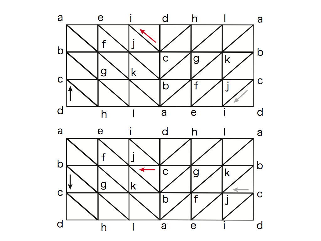
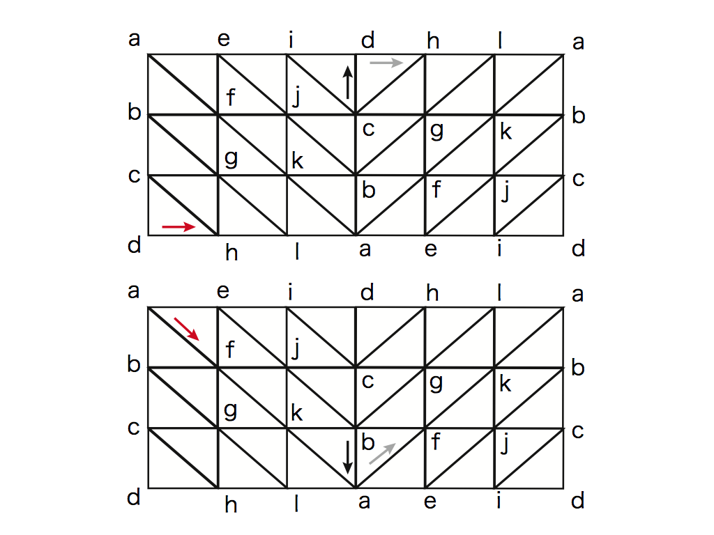
Figure 5: Implementation of quantum walks on the Möbius band.

These figures show implementations of the construction of $\mathcal{K}_{3}$ and S-quantum walks on it. In these figures, the twisted identification of the boundary is imposed on $|ab|,|bc|$ and $|cd|$. This identification changes the rotating direction of triangles. See $|abf|$, for example. $\mathcal{K}_{3}$ can be constructed by this manner.

These figures describe how quantum walks behave on $\mathcal{K}_{3}$. Let black arrows be incident states. The definition of S-quantum walks yields transmitted states drawn by grey arrows, if necessary, via the periodic identification on the boundary. Grey arrows actually describe state on the copy of complexes. True transmitted states are red arrows via identification of the copy.

3.4.2 S-quantum walk on the Möbius band

We set the initial state $\Psi_{0}=\sum_{i=0}^{2}\varphi_{\pi^{i}[abc]}\delta^{(2)}_{\pi^{i}[abc]}+\sum_{i=0}^{2}\varphi_{\pi^{i}[acb]}\delta^{(2)}_{\pi^{i}[acb]}\in\ell^{2}(\tilde{K}_{2})$ at the center of $\mathcal{K}_{3}$, where $\varphi_{\pi^{i}[abc]}=\varphi_{\pi^{i}[acb]}=1/\sqrt{6},\ i=0,1,2$. Let the weight $w(\sigma)$ be

$$w(\sigma_{1}) \equiv\sqrt{0.9/2}\quad\text{ for all $\sigma_{1}\in\tilde{K}_{2}$ with $|\sigma_{1}|$ being a lower triangle},$$

$$w(\sigma_{2}) \equiv\sqrt{1.1/2}\quad\text{ for all $\sigma_{2}\in\tilde{K}_{2}$ with $|\sigma_{2}|$ being an upper triangle}.$$ (3.10)

The S-quantum walk with this weight is shown in Figure 14-(a). We observe that quantum walker goes away from the center drawing spirals. This behavior is completely different from the case of infinite cylinders, although the Möbius band is homologically identical with an infinite cylinder. This observation implies that quantum walks on the Möbius band does not admit localization. This suggestion can be also observed from the viewpoint of the time-averaged probability. Consider the state at the starting simplex $|\sigma_{0}|=|abc|$, which is labelled by $(i,j,k)=(N/2,N/2,0)$, and the adjacent simplex $|\sigma_{0}^{\prime}|$ labelled by $(i,j,k)=(N/2,N/2,1)$. Note that the support of the initial state $\Psi_{0}$ is $|\sigma_{0}|$ and that $|\sigma_{0}|$ is on the central cycle where localization is observed in the case of $\mathcal{K}_{1}$. Figure 15 shows that both $\bar{\mu}_{T}^{(\Psi_{0})}(|\sigma_{0}|)$ and $\bar{\mu}_{T}^{(\Psi_{0})}(|\sigma_{0}^{\prime}|)$ tends to zero as $T\to\infty$.

As a comparison, quantum walks on $\mathcal{K}_{1}$ is shown in Figure 14-(b). In this figure we impose the same initial condition and weights as the case of Figure 14-(a). As we have seen in Subsection 3.2, quantum walks on $\mathcal{K}_{1}$ has localization, which can be seen from the positive probability density at the center in $y$-direction.

Note again that the Möbius band has the identical homology with infinite cylinder. Observations in this subsection imply that more detailed geometric features, like orientation, than homology can affect dynamics of our quantum walks.

4 Conclusion and Discussion

In this paper we constructed a new type of quantum walks on simplicial complexes. We also discussed behavior of our quantum walks, simplicial quantum walks, with numerical simulations. We numerically observe the following.

• The permutation $\pi:[abc]\mapsto[bca]$ induces movable S-quantum walks (Definition 2.14).

• Appropriate choice of weights induce interactive S-quantum walks (Definition 2.15).

• Linear spreading of S-quantum walks happen as in the case of quantum walks on lattices such as $\mathbb{Z}^{d}$.

• S-quantum walks on $\mathcal{K}_{0}$, the triangulation of $\mathbb{R}^{2}$, do not admit localizations. This is completely different from quantum walks on the triangular lattice embedded in $\mathbb{R}^{2}$. In other words, traditional quantum walks on $\mathbb{Z}^{d}$ and simplicial quantum walks exhibit different behavior as traditional multi-dimensional quantum walks.

• Localization occurs when the simplicial complex has non-trivial homological structures, namely, rings or cavities.

• Localizations caused by the second homology classes (i.e. cavities) absorb those by the first homology classes (i.e. rings).

• Localizations depend on the orientability of polyhedra.

Our simplicial quantum walks have the same main features, like linear spreading and localizations, as walks on graphs. In such a sense, our simplicial quantum walks are ones of multi-dimensional analogues of quantum walks on graphs. We also observe different phenomena from quantum walks on graphs, which reflects geometry of simplicial complexes. All observations herein can also hold for quantum walks on multi-dimensional simplicial complexes.

On the other hand, our simplicial quantum walks give us a nontrivial problem concerning exhibition of nontrivial behavior, namely, whether $\pi\in\mathcal{S}_{n+1}$ induces tethered or movable quantum walks. As mentioned in the end of Section 2, an $n$-dimensional quantum walk can be trivial in the sense that $\pi\in\mathcal{S}_{n+1}$ induces tethered quantum walks, if the walk is associated with $\pi\in\mathcal{S}_{n+1}$ whose order is less than $n+1$. Such a phenomenon cannot be seen in typical quantum walks on graphs, such as $2$-state or $3$-state Grover walk on $\mathbb{Z}$. As mentioned above, we numerically observed that $\pi:[abc]\mapsto[bca]$ induces movable quantum walks. Even for permutations of the form (2.1), however, it is in general nontrivial if a given permutation $\pi$ induces movable quantum walks. This classification problem is very important to construct simplicial quantum walks since, as our observations with $n=2$ show, it is intrinsically related to non-triviality of quantum walks. In particular, tethered quantum walks concerns with non-triviality of walks from the viewpoint of shift operators, while non-interactivity concerns with non-triviality from the viewpoint of coin operators.

We end this paper proposing further directions of our arguments.

(1) Characterization of the spectrum of quantum walk $U$ and localization.

The spectrum of $U$ is a core for understanding quantum walks, in particular, related to localization. In [21] and preceding works therein, cycles of graphs can characterize spectrum of $U$ which corresponds to localization. Our numerical results imply that such correspondence are valid for simplicial quantum walks. Our numerical results also show that deeper geometric features of simplicial complexes than graphs, like homology of the higher order and orientations, can affect behavior of quantum walks. One can guess that spectrum of $U$ reveals geometry of underlying spaces as well as multi-dimensional aspect of quantum walks, which will be seen in the forthcoming paper [26].

(2) Asymptotic behavior of S-quantum walks.

As quantum walks on $\mathbb{Z}^{d}$ or graphs, the asymptotic behavior of quantum walks is also the heart for understanding S-quantum walks. The weak convergence of distributions is the key to describe exhibition of linear spreading of quantum walks (e.g. [3]). Fortunately, we numerically observe that the linear spreading happens in many examples. This fact implies that various techniques for the asymptotic behavior of quantum walks on graphs can be also applied to our quantum walks, which will be seen in the forthcoming paper [26].

Appendix A Simplicial complexes and homology groups

We state a quick review of homology of simplicial complexes for readers who are not familiar with it. See e.g. [27] for details.

Definition A.1.

Let $\mathbb{R}^{N}$ be a Euclidean space and $O_{N}$ be the origin of $\mathbb{R}^{N}$. Let $a_{0},a_{1},\cdots,a_{n}\in\mathbb{R}^{N}$ be points so that $n$ vectors $\{\overrightarrow{a_{0}a_{i}}\}_{i=1}^{n}$ are linearly independent. An $n$-simplex is a set $|\sigma|\subset\mathbb{R}^{N}$ given by

$$|\sigma|=\left\{\sum_{i=1}^{n}\lambda_{i}\overrightarrow{a_{0}a_{i}}\mid\lambda_{i}\geq 0,\ \sum_{i=1}^{n}\lambda_{i}=1\right\}.$$

We also write $|\sigma|$ as $|a_{0}a_{1}\cdots a_{n}|$ if we write the dependence of points $\{a_{i}\}_{i=0}^{n}$ explicitly. A $k$-face of an $n$-simplex $|\sigma|=|a_{0}a_{1}\cdots a_{n}|$ is a $k$-simplex $|\tau|$ generated by $k$ points in $\{a_{0}\}_{i=0}^{n}$. In such a case, $|\sigma|$ is called a coface of $|\tau|$. An $(n-1)$-face of an $n$-simplex $\sigma$ is often called a primary face of $\sigma$.

For example, for a given simplex $|\sigma|=|abc|$, edges $|ab|$, $|bc|$ and $|ca|$ are primary faces of $\sigma$. Also, vertices $|a|$, $|b|$ and $|c|$ are $0$-faces of $|\sigma|$. Finally, $|\sigma|$ is a coface of $|a|$, $|b|$, $|c|$, $|ab|$, $|bc|$ and $|ca|$.

Definition A.2.

A simplicial complex $\mathcal{K}$ is the collection of simplices satisfying

• If $|\sigma|\in\mathcal{K}$, then all faces of $|\sigma|$ are also elements in $\mathcal{K}$.

• If $|\sigma_{1}|,|\sigma_{2}|\in\mathcal{K}$ and if $|\sigma_{1}|\cap|\sigma_{2}|\not=\emptyset$, then $|\sigma_{1}|\cap|\sigma_{2}|$ is a face of both $|\sigma_{1}|$ and $|\sigma_{2}|$.

For a given simplicial complex $\mathcal{K}$, the union of all simplices of $\mathcal{K}$ is the polytope of $\mathcal{K}$ and is denoted by $\mathcal{K}$. A set $P$ is a polyhedron if it is the polytope $\mathcal{K}$ of a simplicial complex $\mathcal{K}$.

Let $\mathcal{K}=\{K_{k}\}_{k\geq 0}$ be a simplicial complex, where $K_{k}=\{|\sigma|\in\mathcal{K}\mid|\sigma|\text{ is a $k$-simplex}\}$. If $n=\max\{k\mid K_{k}\not=\emptyset\}<\infty$, then we call $\mathcal{K}$ an $n$-dimensional simplicial complex. For a simplicial complex $\mathcal{K}$ with $\dim\mathcal{K}=n$, its $m$-skeleton is defined by $\mathcal{K}^{(m)}:=\{K_{k}\}_{k\geq 0}^{m}$ for $m\leq n$. For each $|\sigma|\in K_{k}$, we call the number $k$ the dimension of $|\sigma|$. Simplicial complexes admit several classes to be considered.

Definition A.3.

For a simplicial complex $\mathcal{K}$, a facet in $\mathcal{K}$ is a simplex $\sigma\in\mathcal{K}$ which is maximal with respect to the inclusion relation of sets. A simplicial complex $\mathcal{K}$ is pure if all facets in $\mathcal{K}$ have an identical dimension. An $n$-dimensional pure simplicial complex $\mathcal{K}$ is strongly connected if, for each $|\sigma|,|\tau|\in K_{n}$, there is a sequence of $n$-simplices $\{|\sigma_{j}|\}_{j=0}^{k}$ with $|\sigma_{0}|=|\sigma|$ and $|\sigma_{k}|=|\tau|$ such that $|\sigma_{j-1}|\cap|\sigma_{j}|$ is a primary face of $|\sigma_{j-1}|$ and $|\sigma_{j}|$ for $j=1,\cdots,n$.

Remark A.4.

We often call an $(n-1)$-face of an $n$-simplex $|\sigma|$ a facet of $|\sigma|$. It is completely different from facets in simplicial complexes.

The core of homology is to translate geometric objects to algebraic ones in terms of chains.

Definition A.5.

Let $\mathcal{K}$ be a simplicial complex. For each $|\sigma|=|a_{0}a_{1}\cdots a_{k}|\in K_{k}$, the associated $k$-chain is the function $\widehat{|\sigma|}:K_{k}\to\{0,1\}$ given by

$$\widehat{|\sigma|}(|\sigma^{\prime}|):=\begin{cases}1&\text{ if $\sigma^{\prime}=\sigma$}\\ 0&\text{ otherwise}\end{cases}$$

with the following rule: for a permutation $\pi\in S_{k+1}$, identify $\widehat{|\sigma|}(\pi|\sigma|)$ with $(\det\pi)\widehat{|\sigma|}(|\sigma|)$.

Define

$$C_{k}(\mathcal{K}):=\left\{\sum_{j=1}^{k}a_{j}\widehat{|\sigma_{j}|}\mid a_{j}\in\mathbb{Z},\ |\sigma_{j}|\in K_{k}\right\}.$$

This is called $k$-th chain group of $\mathcal{K}$, which is a $\mathbb{Z}$-module.

Definition A.6.

For $|\sigma|=|a_{0}a_{1}\cdots a_{k}|\in K_{k}$, define the boundary $\partial\widehat{|\sigma|}$ of the chain $\widehat{|\sigma|}$ by

$$\partial_{k}\widehat{|\sigma|}:=\sum_{j=0}^{k}(-1)^{j}\widehat{|\cdots a_{j-1}a_{j+1}\cdots|},$$

which is an element in $C_{k-1}$. Extending linearly this definition, we obtain a linear map $\partial_{k}:C_{k}(\mathcal{K})\to C_{k-1}(\mathcal{K})$. This map is called ($k$-th) boundary map of $\mathcal{K}$.

The important property of boundary maps is the following.

Proposition A.7.

$\partial_{k}\circ\partial_{k+1}=0:C_{k+1}(\mathcal{K})\to C_{k-1}(\mathcal{K})$.

A pair $\{C_{k}(\mathcal{K}),\partial_{k}\}_{k\in\mathbb{Z}}$ consisting of sequences of chain groups and boundary maps is called a chain complex of $\mathcal{K}$. Then we are ready to define homology groups.

Definition A.8.

For a simplicial complex $\mathcal{K}$, we define

$$Z_{k}(\mathcal{K}):={\rm Ker}\partial_{k},\quad B_{k}(\mathcal{K}):={\rm Im}\partial_{k+1}.$$

Both are submodules of $C_{k}(\mathcal{K})$. An element in $Z_{k}(\mathcal{K})$ is called a $k$-cycle and an element in $B_{k}(\mathcal{K})$ is called a $k$-boundary. Thanks to Proposition A.7, $B_{k}(\mathcal{K})$ is a submodule of $Z_{k}(\mathcal{K})$. Thus the quotient module

$$H_{k}(\mathcal{K}):=Z_{k}(\mathcal{K})/B_{k}(\mathcal{K})$$

can be considered. This quotient group is called the $k$-th homology group of $\mathcal{K}$. Roughly speaking, the $k$-th homology group describe the information of $k$-dimensional holes in $\mathcal{K}$.

The simple example of homology is shown in Figure 6.

(a)

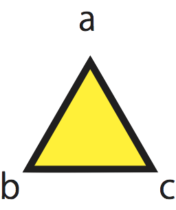
(b)

Figure 6: The first homology class : a simple example.

(a). A triangle without any $2$-simplices. In this case, the chain $\widehat{|ab|}+\widehat{|bc|}+\widehat{|ca|}$ becomes a $1$-cycle. Since no $2$-simplices exist, this $1$-cycle defines a generator of the first homology group, which indicates that this triangle has a hole.
(b). A triangle with a $2$-simplex $|abc|$. In this case, the chain $\widehat{|ab|}+\widehat{|bc|}+\widehat{|ca|}$ becomes a $1$-cycle. On the other hand, this $1$-cycle is also the boundary, which follows from $\widehat{|ab|}+\widehat{|bc|}+\widehat{|ca|}=\partial_{2}(\widehat{|abc|})$. This fact implies that this filled triangle has the trivial first homology group, in other words, the filled triangle does not have any holes.

Appendix B Implementations: time evolution of the S-quantum walk on an infinite cylinder with a tetrahedron

In this section we describe concrete implementations of time evolutions of S-quantum walk on $\mathcal{K}_{2}$, in particular, on and around tetrahedron drawn in Figure 7. On the other region, such evolutions follow from those on $\mathcal{K}_{0}$ discussed in Subsection 3.1.1. All labeling of simplices and bases on them are drawn in Figure 7 and 8, respectively. Readers should refer to descriptions in these figures to study time evolutions stated below.

For the notation rule stated in Remark 3.1, we use bold-letter labelings shown in Figure 7 instead of integer indices. By following the definition of $U$, the evolution of base elements on the 2-simplex ${\bf x}\in\{{\bf a},{\bf b},{\bf c},{\bf A},{\bf B},{\bf C},{\bf D}\}$ is given in Subsections B.1 and B.2.

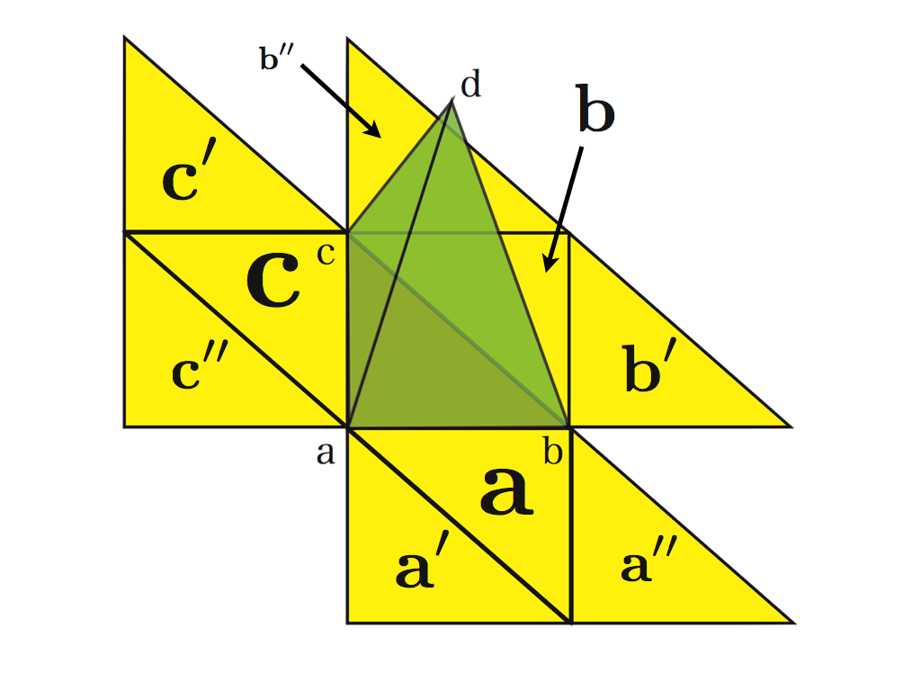
Figure 7: Labeling of simplices around tetrahedron in $\mathcal{K}_{2}$

A tetrahedron is put on the infinite cylinder $\mathcal{K}_{1}$. In this figure we put a tetrahedron, colored by green, on ${\bf A}\equiv|abc|$. As stated in Figure 4-(a) the base element on ${\bf A}$ is determined by

$$\delta_{{\bf A},0}=\delta^{(2)}_{[abc]},\ \delta_{{\bf A},1}=\delta^{(2)}_{[bca]},\ \delta_{{\bf A},2}=\delta^{(2)}_{[cab]},\ \delta_{{\bf A},3}=\delta^{(2)}_{[acb]},\ \delta_{{\bf A},4}=\delta^{(2)}_{[cba]},\ \delta_{{\bf A},5}=\delta^{(2)}_{[bac]}.$$

Simplices on the tetrahedron are labeled by ${\bf B}\equiv|abd|$, ${\bf C}\equiv|bcd|$ and ${\bf D}\equiv|cad|$. See also Figure 8. Simplices which have effects from the tetrahedron are labeled by a, b and c.

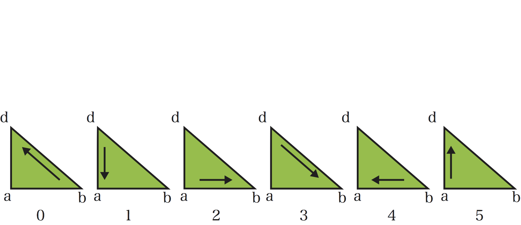
(a)

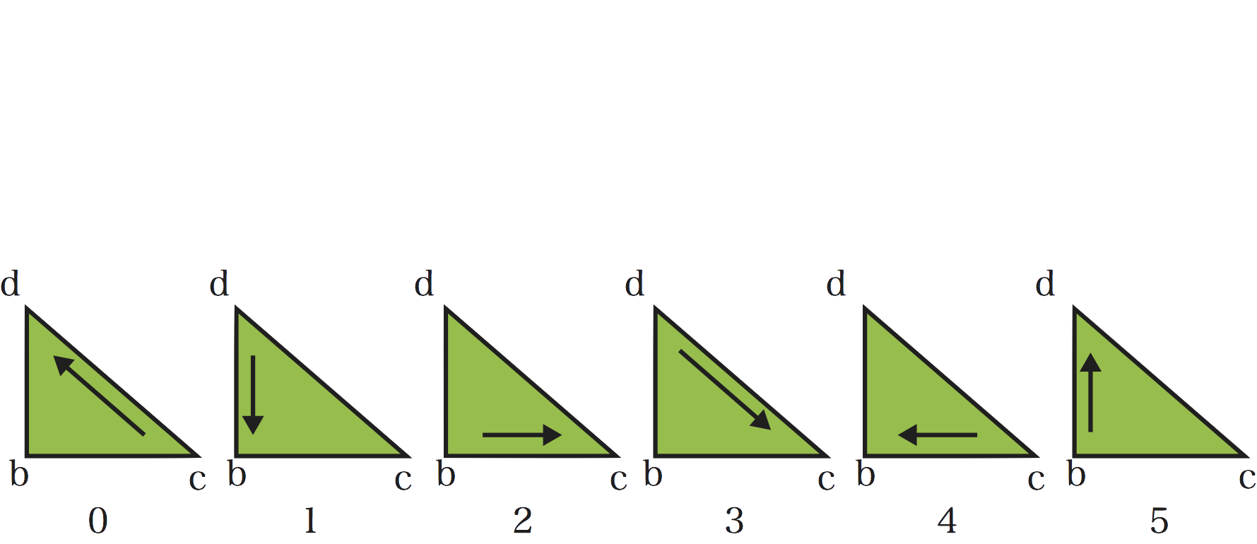
(b)

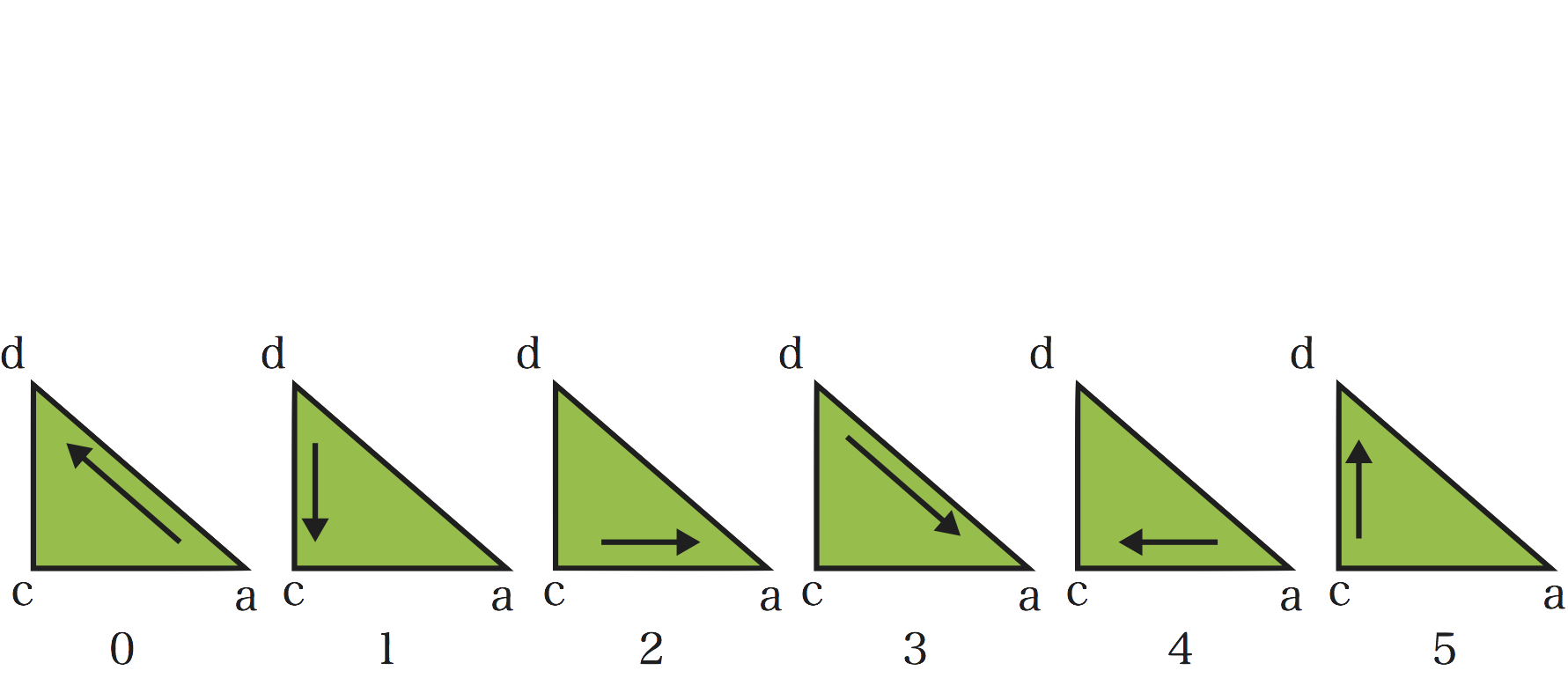
(c)

Figure 8: Labeling of bases on the tetrahedron

Figures here denote the graphical representations of the following bases for $l\in\{0,1,2,3,4,5\}$. Labelings of B, C and D are followed by Figure 7. (a): $\delta_{{\bf B},l}$. (b): $\delta_{{\bf C},l}$. (c): $\delta_{{\bf D},l}$.

B.1 $2$-simplices around tetrahedron

Case 1: $2$-simplex labeled a (Figure 7 and 8)

$$\begin{pmatrix}\delta_{{\bf a},0}\\ \delta_{{\bf a},1}\\ \delta_{{\bf a},2}\\ \delta_{{\bf a},3}\\ \delta_{{\bf a},4}\\ \delta_{{\bf a},5}\end{pmatrix} \mapsto\begin{pmatrix}(2|w_{{\bf a},0}|^{2}-1)\cdot\delta_{{\bf a},1}\\ (2|w_{{\bf a},1}|^{2}-1)\cdot\delta_{{\bf a},2}\\ (2|w_{{\bf a},2}|^{2}-1)\cdot\delta_{{\bf a},0}\\ (2|w_{{\bf a},3}|^{2}-1)\cdot\delta_{{\bf a},4}\\ (2|w_{{\bf a},4}|^{2}-1)\cdot\delta_{{\bf a},5}\\ (2|w_{{\bf a},5}|^{2}-1)\cdot\delta_{{\bf a},3}\end{pmatrix}+\begin{pmatrix}2\overline{w_{{\bf a},0}}w_{{\bf A},4}\cdot\delta_{{\bf A},5}\\ 2\overline{w_{{\bf a},1}}w_{{\bf a}^{\prime},3}\cdot\delta_{{\bf a}^{\prime},4}\\ 2\overline{w_{{\bf a},2}}w_{{\bf a}^{\prime\prime},5}\cdot\delta_{{\bf a}^{\prime\prime},3}\\ 2\overline{w_{{\bf a},3}}w_{{\bf A},2}\cdot\delta_{{\bf A},0}\\ 2\overline{w_{{\bf a},4}}w_{{\bf a}^{\prime\prime},1}\cdot\delta_{{\bf a}^{\prime\prime},2}\\ 2\overline{w_{{\bf a},5}}w_{{\bf a}^{\prime},0}\cdot\delta_{{\bf a}^{\prime},1}\end{pmatrix}+\begin{pmatrix}2\overline{w_{{\bf a},0}}w_{{\bf B},4}\cdot\delta_{{\bf B},5}\\ 0\\ 0\\ 2\overline{w_{{\bf a},3}}w_{{\bf B},2}\cdot\delta_{{\bf B},0}\\ 0\\ 0\end{pmatrix}.$$

Case 2: $2$-simplex labeled b (Figure 7 and 8)

$$\begin{pmatrix}\delta_{{\bf b},0}\\ \delta_{{\bf b},1}\\ \delta_{{\bf b},2}\\ \delta_{{\bf b},3}\\ \delta_{{\bf b},4}\\ \delta_{{\bf b},5}\end{pmatrix}\mapsto\begin{pmatrix}(2|w_{{\bf b},0}|^{2}-1)\cdot\delta_{{\bf b},1}\\ (2|w_{{\bf b},1}|^{2}-1)\cdot\delta_{{\bf b},2}\\ (2|w_{{\bf b},2}|^{2}-1)\cdot\delta_{{\bf b},0}\\ (2|w_{{\bf b},3}|^{2}-1)\cdot\delta_{{\bf b},4}\\ (2|w_{{\bf b},4}|^{2}-1)\cdot\delta_{{\bf b},5}\\ (2|w_{{\bf b},5}|^{2}-1)\cdot\delta_{{\bf b},3}\end{pmatrix}+\begin{pmatrix}2\overline{w_{{\bf b},0}}w_{{\bf b}^{\prime\prime},4}\cdot\delta_{{\bf b}^{\prime\prime},5}\\ 2\overline{w_{{\bf b},1}}w_{{\bf A},3}\cdot\delta_{{\bf A},4}\\ 2\overline{w_{{\bf b},2}}w_{{\bf b}^{\prime},5}\cdot\delta_{{\bf b}^{\prime},3}\\ 2\overline{w_{{\bf b},3}}w_{{\bf b}^{\prime\prime},2}\cdot\delta_{{\bf b}^{\prime\prime},0}\\ 2\overline{w_{{\bf b},4}}w_{{\bf b}^{\prime},1}\cdot\delta_{{\bf b}^{\prime},2}\\ 2\overline{w_{{\bf b},5}}w_{{\bf A},0}\cdot\delta_{{\bf A},1}\end{pmatrix}+\begin{pmatrix}0\\ 2\overline{w_{{\bf b},1}}w_{{\bf C},4}\cdot\delta_{{\bf C},5}\\ 0\\ 0\\ 0\\ 2\overline{w_{{\bf b},5}}w_{{\bf C},2}\cdot\delta_{{\bf C},0}\end{pmatrix}.$$

Case 3: $2$-simplex labeled c (Figure 7 and 8)

$$\begin{pmatrix}\delta_{{\bf c},0}\\ \delta_{{\bf c},1}\\ \delta_{{\bf c},2}\\ \delta_{{\bf c},3}\\ \delta_{{\bf c},4}\\ \delta_{{\bf c},5}\end{pmatrix} \mapsto\begin{pmatrix}(2|w_{{\bf c},0}|^{2}-1)\cdot\delta_{{\bf c},1}\\ (2|w_{{\bf c},1}|^{2}-1)\cdot\delta_{{\bf c},2}\\ (2|w_{{\bf c},2}|^{2}-1)\cdot\delta_{{\bf c},0}\\ (2|w_{{\bf c},3}|^{2}-1)\cdot\delta_{{\bf c},4}\\ (2|w_{{\bf c},4}|^{2}-1)\cdot\delta_{{\bf c},5}\\ (2|w_{{\bf c},5}|^{2}-1)\cdot\delta_{{\bf c},3}\end{pmatrix}+\begin{pmatrix}2\overline{w_{{\bf c},0}}w_{{\bf c}^{\prime},4}\cdot\delta_{{\bf c}^{\prime},5}\\ 2\overline{w_{{\bf c},1}}w_{{\bf c}^{\prime\prime},3}\cdot\delta_{{\bf c}^{\prime\prime},4}\\ 2\overline{w_{{\bf c},2}}w_{{\bf A},5}\cdot\delta_{{\bf A},3}\\ 2\overline{w_{{\bf c},3}}w_{{\bf c}^{\prime},2}\cdot\delta_{{\bf c}^{\prime},0}\\ 2\overline{w_{{\bf c},4}}w_{{\bf A},1}\cdot\delta_{{\bf A},2}\\ 2\overline{w_{{\bf c},5}}w_{{\bf c}^{\prime\prime},0}\cdot\delta_{{\bf c}^{\prime\prime},1}\end{pmatrix}+\begin{pmatrix}0\\ 0\\ 2\overline{w_{{\bf c},2}}w_{{\bf D},4}\cdot\delta_{{\bf D},5}\\ 0\\ 2\overline{w_{{\bf c},4}}w_{{\bf D},2}\cdot\delta_{{\bf D},0}\\ 0\end{pmatrix}.$$

B.2 $2$-simplices on tetrahedron

Case 1: $2$-simplex labeled A (Figure 7 and 8)

$$\begin{pmatrix}\delta_{{\bf A},0}\\ \delta_{{\bf A},1}\\ \delta_{{\bf A},2}\\ \delta_{{\bf A},3}\\ \delta_{{\bf A},4}\\ \delta_{{\bf A},5}\end{pmatrix} \mapsto\begin{pmatrix}(2|w_{{\bf A},0}|^{2}-1)\cdot\delta_{{\bf A},1}\\ (2|w_{{\bf A},1}|^{2}-1)\cdot\delta_{{\bf A},2}\\ (2|w_{{\bf A},2}|^{2}-1)\cdot\delta_{{\bf A},0}\\ (2|w_{{\bf A},3}|^{2}-1)\cdot\delta_{{\bf A},4}\\ (2|w_{{\bf A},4}|^{2}-1)\cdot\delta_{{\bf A},5}\\ (2|w_{{\bf A},5}|^{2}-1)\cdot\delta_{{\bf A},3}\end{pmatrix}+\begin{pmatrix}2\overline{w_{{\bf A},0}}w_{{\bf b},5}\cdot\delta_{{\bf b},3}\\ 2\overline{w_{{\bf A},1}}w_{{\bf c},4}\cdot\delta_{{\bf c},5}\\ 2\overline{w_{{\bf A},2}}w_{{\bf a},3}\cdot\delta_{{\bf a},4}\\ 2\overline{w_{{\bf A},3}}w_{{\bf b},1}\cdot\delta_{{\bf b},2}\\ 2\overline{w_{{\bf A},4}}w_{{\bf a},0}\cdot\delta_{{\bf a},1}\\ 2\overline{w_{{\bf A},5}}w_{{\bf c},2}\cdot\delta_{{\bf c},0}\end{pmatrix}+\begin{pmatrix}2\overline{w_{{\bf A},0}}w_{{\bf C},2}\cdot\delta_{{\bf C},0}\\ 2\overline{w_{{\bf A},1}}w_{{\bf D},2}\cdot\delta_{{\bf D},0}\\ 2\overline{w_{{\bf A},2}}w_{{\bf B},2}\cdot\delta_{{\bf B},0}\\ 2\overline{w_{{\bf A},3}}w_{{\bf C},4}\cdot\delta_{{\bf C},5}\\ 2\overline{w_{{\bf A},4}}w_{{\bf B},4}\cdot\delta_{{\bf B},5}\\ 2\overline{w_{{\bf A},5}}w_{{\bf D},4}\cdot\delta_{{\bf D},5}\end{pmatrix}.$$

Case 2: $2$-simplex labeled B (Figure 7 and 8)

$$\begin{pmatrix}\delta_{{\bf B},0}\\ \delta_{{\bf B},1}\\ \delta_{{\bf B},2}\\ \delta_{{\bf B},3}\\ \delta_{{\bf B},4}\\ \delta_{{\bf B},5}\end{pmatrix} \mapsto\begin{pmatrix}(2|w_{{\bf B},0}|^{2}-1)\cdot\delta_{{\bf B},1}\\ (2|w_{{\bf B},1}|^{2}-1)\cdot\delta_{{\bf B},2}\\ (2|w_{{\bf B},2}|^{2}-1)\cdot\delta_{{\bf B},0}\\ (2|w_{{\bf B},3}|^{2}-1)\cdot\delta_{{\bf B},4}\\ (2|w_{{\bf B},4}|^{2}-1)\cdot\delta_{{\bf B},5}\\ (2|w_{{\bf B},5}|^{2}-1)\cdot\delta_{{\bf B},3}\end{pmatrix}+\begin{pmatrix}0\\ 0\\ 2\overline{w_{{\bf B},2}}w_{{\bf a},6}\cdot\delta_{{\bf a},4}\\ 0\\ 2\overline{w_{{\bf B},4}}w_{{\bf a},0}\cdot\delta_{{\bf a},1}\\ 0\end{pmatrix}+\begin{pmatrix}2\overline{w_{{\bf B},0}}w_{{\bf C},5}\cdot\delta_{{\bf C},3}\\ 2\overline{w_{{\bf B},1}}w_{{\bf D},3}\cdot\delta_{{\bf D},4}\\ 2\overline{w_{{\bf B},2}}w_{{\bf A},2}\cdot\delta_{{\bf A},0}\\ 2\overline{w_{{\bf B},3}}w_{{\bf C},1}\cdot\delta_{{\bf C},2}\\ 2\overline{w_{{\bf B},4}}w_{{\bf A},4}\cdot\delta_{{\bf A},5}\\ 2\overline{w_{{\bf B},5}}w_{{\bf D},0}\cdot\delta_{{\bf D},1}\end{pmatrix}.$$

Case 3: $2$-simplex labeled C (Figure 7 and 8)

$$\begin{pmatrix}\delta_{{\bf C},0}\\ \delta_{{\bf C},1}\\ \delta_{{\bf C},2}\\ \delta_{{\bf C},3}\\ \delta_{{\bf C},4}\\ \delta_{{\bf C},5}\end{pmatrix} \mapsto\begin{pmatrix}(2|w_{{\bf C},0}|^{2}-1)\cdot\delta_{{\bf C},1}\\ (2|w_{{\bf C},1}|^{2}-1)\cdot\delta_{{\bf C},2}\\ (2|w_{{\bf C},2}|^{2}-1)\cdot\delta_{{\bf C},0}\\ (2|w_{{\bf C},3}|^{2}-1)\cdot\delta_{{\bf C},4}\\ (2|w_{{\bf C},4}|^{2}-1)\cdot\delta_{{\bf C},5}\\ (2|w_{{\bf C},5}|^{2}-1)\cdot\delta_{{\bf C},3}\end{pmatrix}+\begin{pmatrix}0\\ 0\\ 2\overline{w_{{\bf C},2}}w_{{\bf b},5}\cdot\delta_{{\bf b},3}\\ 0\\ 2\overline{w_{{\bf C},4}}w_{{\bf b},1}\cdot\delta_{{\bf b},2}\\ 0\end{pmatrix}+\begin{pmatrix}2\overline{w_{{\bf C},0}}w_{{\bf D},5}\cdot\delta_{{\bf D},3}\\ 2\overline{w_{{\bf C},1}}w_{{\bf B},3}\cdot\delta_{{\bf B},4}\\ 2\overline{w_{{\bf C},2}}w_{{\bf A},0}\cdot\delta_{{\bf A},1}\\ 2\overline{w_{{\bf C},3}}w_{{\bf D},1}\cdot\delta_{{\bf D},2}\\ 2\overline{w_{{\bf C},4}}w_{{\bf A},3}\cdot\delta_{{\bf A},4}\\ 2\overline{w_{{\bf C},5}}w_{{\bf B},0}\cdot\delta_{{\bf B},1}\end{pmatrix}.$$

Case 4: $2$-simplex labeled D (Figure 7 and 8)

$$\begin{pmatrix}\delta_{{\bf D},0}\\ \delta_{{\bf D},1}\\ \delta_{{\bf D},2}\\ \delta_{{\bf D},3}\\ \delta_{{\bf D},4}\\ \delta_{{\bf D},5}\end{pmatrix} \mapsto\begin{pmatrix}(2|w_{{\bf D},0}|^{2}-1)\cdot\delta_{{\bf D},1}\\ (2|w_{{\bf D},1}|^{2}-1)\cdot\delta_{{\bf D},2}\\ (2|w_{{\bf D},2}|^{2}-1)\cdot\delta_{{\bf D},0}\\ (2|w_{{\bf D},3}|^{2}-1)\cdot\delta_{{\bf D},4}\\ (2|w_{{\bf D},4}|^{2}-1)\cdot\delta_{{\bf D},5}\\ (2|w_{{\bf D},5}|^{2}-1)\cdot\delta_{{\bf D},3}\end{pmatrix}+\begin{pmatrix}0\\ 0\\ 2\overline{w_{{\bf D},2}}w_{{\bf c},4}\cdot\delta_{{\bf c},5}\\ 0\\ 2\overline{w_{{\bf D},2}}w_{{\bf c},2}\cdot\delta_{{\bf c},0}\\ 0\end{pmatrix}+\begin{pmatrix}2\overline{w_{{\bf D},0}}w_{{\bf B},5}\cdot\delta_{{\bf B},3}\\ 2\overline{w_{{\bf D},1}}w_{{\bf C},3}\cdot\delta_{{\bf C},4}\\ 2\overline{w_{{\bf D},2}}w_{{\bf A},1}\cdot\delta_{{\bf A},2}\\ 2\overline{w_{{\bf D},3}}w_{{\bf B},1}\cdot\delta_{{\bf B},2}\\ 2\overline{w_{{\bf D},2}}w_{{\bf A},5}\cdot\delta_{{\bf A},3}\\ 2\overline{w_{{\bf D},5}}w_{{\bf C},0}\cdot\delta_{{\bf C},1}\end{pmatrix}.$$

Appendix C Figures: behavior of S-quantum walks on simplicial complexes

(a). Probability density distribution after $120$ steps of the S-quantum walk with the weight (3.1). Initial state at $|abc|$, $a=(0,0)\in\mathbb{R}^{2}$, $b=(1,0)\in\mathbb{R}^{2}$, $c=(0,1)\in\mathbb{R}^{2}$ moves in monotone directions. This is a typical example of the non-interactive quantum walk.

(b). Probability density distribution after $120$ steps of the S-quantum walk with the weight (3.2). Initial state at $|abc|$ draws the hexagram.

(c). Probability density distribution after $120$ steps of the S-quantum walk with the weight (3.3). Initial state at $|abc|$ draws the hexagram but the speed of the spread is slower than the case (b).

In all cases localization cannot be observed, which is the big difference from the quantum walk on crystal lattices [21].

Probability density distribution after $120$ steps of the S-quantum walk with the weight (3.2) and the following initial states.

(a). The initial state is $\Psi_{0}=\delta^{(2)}_{[abc]}$, where $a=(0,0)\in\mathbb{R}^{2}$, $b=(1,0)\in\mathbb{R}^{2}$, $c=(0,1)\in\mathbb{R}^{2}$. The S-quantum walk monotone spreads drawing triangle with high probability in one direction.

(b). The initial state is $\Psi_{0}=\frac{1}{\sqrt{2}}\delta^{(2)}_{[abc]}+\frac{1}{\sqrt{2}}\delta^{(2)}_{[bca]}$. The S-quantum walk spreads drawing triangle with high probability in two directions.

(c). The initial state is $\Psi_{0}=\frac{1}{\sqrt{2}}\delta^{(2)}_{[abc]}+\frac{1}{\sqrt{2}}\delta^{(2)}_{[acb]}$. The S-quantum walk spreads drawing hexagram with high probability in two directions.

(a). Time evolution of $V_{n}/n^{2}$ for the Hadamard walk on $\mathbb{Z}^{2}$ (e.g. [3]). The value of $V_{n}/n^{2}$ converges to $\approx 0.01719$.

(b). Time evolution of $V_{n}/n^{2}$ for the S-quantum walk on $\mathcal{K}_{0}$ with the weight (3.2). The value of $V_{n}/n^{2}$ converges to $\approx 0.01671$.

(c). Time evolution of $V_{n}/n^{2}$ for the S-quantum walk on $\mathcal{K}_{1}$ with the weight (3.1). The value of $V_{n}/n^{2}$ converges to $\approx 0.05545$.

(d). Time evolution of $V_{n}/n^{2}$ for the S-quantum walk on $\mathcal{K}_{1}$ with the weight (3.2). The value of $V_{n}/n^{2}$ converges to $\approx 0.02941$.

(a): Localization at the origin.
(b): Convergence of variance of the quantum walk $\Psi_{n}/n$. Row: time. Column: the value of the variance $V_{n}/n^{2}$ at the time $n$.

Figures (a) and (b) depict probability after 2000 steps of the S-quantum walk on $\mathcal{K}_{1}$ with the weights (3.1) and (3.2), respectively. Figure (c) depict probability after 2000 steps of the S-quantum walk on $\mathcal{K}_{2}$ with the weight (3.9). In all cases the initial state $\Psi_{0}$ is given by (3.7) (see also Figure 7).

(a). Initial state $\Psi_{0}$ moves in two infinite directions as well as staying on the cycle where the starting simplex is located with a positive probability. See also the graph “cylinder-transmit” in Figure 15. This is an example of the non-interactive quantum walk.

(b). Initial state $\Psi_{0}$ moves in two infinite directions as well as staying on the cycle where the starting simplex is located with a positive probability, as in the case of (a). See also the graph “cylinder-hetero” in Figure 15.

(c). Localization occurs on the tetrahedron, while localization on the circle observed in the case of $\mathcal{K}_{1}$ is absorbed by the tetrahedron. See also the graphs “tetra-on” and “tetra-off” in Figure 15.

(a). Probability density distribution after $2100$ steps of the S-quantum walk on $\mathcal{K}_{3}$ with the weight (3.10). Although the initial state exists only on the center of $\mathcal{K}_{3}$, quantum walker slides away from the center in $y$-coordinate. This implies that no localization can occur on $\mathcal{K}_{3}$, which reflects the geometry of $\mathcal{K}_{3}$ that the Möbius band is non-orientable.

(b). Probability density distribution after $2100$ steps of the S-quantum walk on $\mathcal{K}_{1}$ with the weight (3.10). The initial state is the same as (a). In this case, localization can occur.

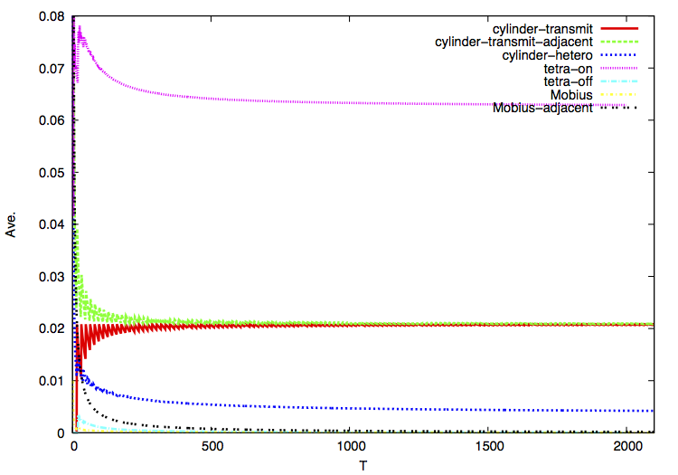
Figure 15: Time-averaged probability of S-quantum walks on simplices

Each graph denotes the time-averaged probability $\bar{\mu}_{T}(|\sigma|)$ at time $T$ and at $|\sigma|\in K_{2}$. Let $|\sigma_{0}|$ be the support of the initial state $\Psi_{0}$ discussed in Section 3, labelled by $(i,j,k)=(N/2,N/2,0)$.

• “cylinder-transmit” (red) denotes $\bar{\mu}_{T}^{(\Psi_{0})}(|\sigma_{0}|)$ for S-quantum walk on $\mathcal{K}_{1}$ with the weight (3.1).

• “cylinder-transmit-adjacent” (green) denotes $\bar{\mu}_{T}^{(\Psi_{0})}(|\sigma|)$ at $\sigma\in K_{2}$ labelled by $(i,j,k)=(N/2-1,N/2,0)$, which is on the central cycle, for S-quantum walk on $\mathcal{K}_{1}$ with the weight (3.1).

• “cylinder-hetero” (blue) denotes $\bar{\mu}_{T}^{(\Psi_{0})}(|\sigma_{0}|)$ for S-quantum walk on $\mathcal{K}_{1}$ with the weight (3.2).

• “tetra-on” (purple) denotes $\bar{\mu}_{T}^{(\Psi_{0})}(|\sigma_{0}|)$ for S-quantum walk on $\mathcal{K}_{2}$ with the weight (3.9). Note that $\sigma$ is a part of the tetrahedron in $\mathcal{K}_{2}$.

• “tetra-off” (sky blue) denotes $\bar{\mu}_{T}^{(\Psi_{0})}(|\sigma|)$ at $|\sigma|\in K_{2}$ labelled by $(i,j,k)=(N/2-1,N/2,0)$ for S-quantum walk on $\mathcal{K}_{2}$ with the weight (3.9). Note that $\sigma$ is on the central cycle but off the tetrahedron in $\mathcal{K}_{2}$. Comparing with “cylinder-transmit-adjacent”, localization is not exhibited in this case.

• “Mobius” (yellow) denotes $\bar{\mu}_{T}^{(\Psi_{0})}(|\sigma_{0}|)$ for S-quantum walk on $\mathcal{K}_{3}$ with the weight (3.10).

• “Mobius-adjacent” (black) denotes $\bar{\mu}_{T}^{(\Psi_{0})}(|\sigma|)$ at $|\sigma|\in K_{2}$ labelled by $(i,j,k)=(N/2,N/2,1)$ for S-quantum walk on $\mathcal{K}_{3}$ with the weight (3.10).

In all cases which localization occurs, $\bar{\mu}_{T}^{(\Psi_{0})}(|\sigma|)$ converges to a positive value as $T\to\infty$, while in other cases $\bar{\mu}_{T}^{(\Psi_{0})}(|\sigma|)$ tends to zero.

References

- [1] S.P. Gudder. Quantum probability. Probability and Mathematical Statistics. Academic Press, Inc., Boston, MA, 1988.
- [2] R.P. Feynman and A.R. Hibbs. Quantum mechanics and path integrals. Dover Publications, Inc., Mineola, NY, emended edition, 2010. Emended and with a preface by Daniel F. Styer.
- [3] N. Konno. Quantum random walks in one dimension. Quantum Inf. Process., Vol. 1, No. 5, pp. 345–354 (2003), 2002.
- [4] A. Ambainis. Quantum walks and their algorithmic applications. International Journal of Quantum Information, Vol. 1, No. 04, pp. 507–518, 2003.
- [5] N. Konno. Quantum walks. In Quantum potential theory, Vol. 1954 of Lecture Notes in Math., pp. 309–452. Springer, Berlin, 2008.
- [6] A. Ambainis. Quantum walk algorithm for element distinctness. SIAM J. Comput., Vol. 37, No. 1, pp. 210–239 (electronic), 2007.
- [7] A. Ambainis, J. Kempe and A. Rivosh. Coins make quantum walks faster. In Proceedings of the Sixteenth Annual ACM-SIAM Symposium on Discrete Algorithms, pp. 1099–1108 (electronic). ACM, New York, 2005.
- [8] N. Shenvi, J. Kempe and K.B. Whaley. Quantum random-walk search algorithm. Physical Review A, Vol. 67, No. 5, p. 052307, 2003.
- [9] C.M. Chandrashekar, S. Banerjee and R. Srikanth. Relationship between quantum walks and relativistic quantum mechanics. Physical Review A, Vol. 81, No. 6, p. 062340, 2010.
- [10] F.W. Strauch. Relativistic effects and rigorous limits for discrete- and continuous-time quantum walks. J. Math. Phys., Vol. 48, No. 8, pp. 082102, 27, 2007.
- [11] M. Karski, L.Förster, J.-M. Choi, A. Steffen, W. Alt, D. Meschede and A. Widera. Quantum walk in position space with single optically trapped atoms. Science, Vol. 325, No. 5937, pp. 174–177, 2009.
- [12] L. Matsuoka and K. Yokoyama. Physical implementation of quantum cellular automaton in a diatomic molecule. Journal of Computational and Theoretical Nanoscience, Vol. 10, No. 7, pp. 1617–1620, 2013.
- [13] F. Zähringer, G. Kirchmair, R. Gerritsma, E. Solano, R. Blatt and C.F. Roos. Realization of a quantum walk with one and two trapped ions. Physical review letters, Vol. 104, No. 10, p. 100503, 2010.
- [14] J. Wang and K. Manouchehri. Physical implementation of quantum walks. Springer, 2013.
- [15] S. D. Berry, P. Bourke and J.B. Wang. qwviz: Visualisation of quantum walks on graphs. Computer Physics Communications, Vol. 182, No. 10, pp. 2295–2302, 2011.
- [16] J. Watrous. Quantum simulations of classical random walks and undirected graph connectivity. In Computational Complexity, 1999. Proceedings. Fourteenth Annual IEEE Conference on, pp. 180–187. IEEE, 1999.
- [17] Yu. Higuchi, N. Konno, I. Sato and E. Segawa. Quantum graph walks I: Mapping to quantum walks. Yokohama Math. J., Vol. 59, pp. 33–55, 2013.
- [18] M. Szegedy. Quantum speed-up of markov chain based algorithms. In Foundations of Computer Science, 2004. Proceedings. 45th Annual IEEE Symposium on, pp. 32–41. IEEE, 2004.
- [19] G.D. Paparo and M.A. Martin-Delgado. Google in a quantum network. Scientific reports, Vol. 2, , 2012.
- [20] G.D. Paparo, M. Müller, F. Comellas and M.A. Martin-Delgado. Quantum google in a complex network. Scientific reports, Vol. 3, , 2013.
- [21] Yu. Higuchi, N. Konno, I. Sato and E. Segawa. Spectral and asymptotic properties of Grover walks on crystal lattices. J. Funct. Anal., Vol. 267, No. 11, pp. 4197–4235, 2014.
- [22] M.A. Nielsen and I.L. Chuang. Quantum computation and quantum information. Cambridge university press, 2010.
- [23] D.A. Meyer. From quantum cellular automata to quantum lattice gases. J. Statist. Phys., Vol. 85, No. 5-6, pp. 551–574, 1996.
- [24] B. Tregenna, W. Flanagan, R. Maile and V. Kendon. Controlling discrete quantum walks: coins and initial states. New Journal of Physics, Vol. 5, No. 1, p. 83, 2003.
- [25] J.W. Milnor and J.D. Stasheff. Characteristic classes. Princeton University Press, Princeton, N. J.; University of Tokyo Press, Tokyo, 1974. Annals of Mathematics Studies, No. 76.
- [26] K. Matsue, O. Ogurisu and E. Segawa. Quantum walks on cubical sets : Construction and asymptotic behavior on , in preparation.
- [27] T. Kaczynski, K. Mischaikow and M. Mrozek. Computational homology, Vol. 157 of Applied Mathematical Sciences. Springer-Verlag, New York, 2004.