Entropy production of entirely diffusional Laplacian transfer and the possible role of fragmentation of the boundaries

Abstract

The entropy production and the variational functional of a Laplacian diffusional field around the first four fractal iterations of a linear self-similar tree (von Koch curve) is studied analytically and detailed predictions are stated. In a next stage, these predictions are confronted with results from numerical resolution of the Laplace equation by means of Finite Elements computations. After a brief review of the existing results, the range of distances near the geometric irregularity, the so-called ”Near Field”, a situation never studied in the past, is treated exhaustively. We notice here that in the Near Field, the usual notion of the active zone approximation introduced by Sapoval et al.^1,2 is strictly inapplicable. The basic new result is that the validity of the active-zone approximation based on irreversible thermodynamics is confirmed in this limit, and this implies a new interpretation of this notion for Laplacian diffusional fields.

Keywords: Diffusion; Entropy Production; Fractals; Near Field; Laplacian Fields.

I Introduction

On the past decade, an important field of interdisciplinary research has been developed based on new geometry concepts, namely ”the fractal” geometry of nature, pioneered by Benoit B. Mandelbrot. The fractal geometry approximates well enough the naturally discovered disordered morphologies. For instance, the terminal part of the respiratory system of mammals, biological membranes, porous electrodes or catalysts, provide some characteristic examples^3-12.

This implies a direct link to Laplacian transfer, as one could mention that under ordinary conditions many familiar transport phenomena such as diffusion and heat conduction are described in the steady state by Laplacian fields. The Laplace equation is a linear equation, however the complexity of the problem is due to the geometrical irregularities of the boundaries. Due to this fact, an important number of studies on the distribution of Laplacian fields around geometrically irregular - and eventually fractal - objects, have been justified^1,13-18.

An old mathematical conjecture states that the Laplacian field around a fractal object in two dimensions is itself of multifractal nature. This conjecture, after Makarov’s theorem is a mathematical fact. In a paper considered classical by now, B.B. Mandelbrot explored for the first time in detail the Laplacian field around a deterministic self-similar tree with his famous ”zebroide” (logarithmic) representation¹⁹. This work was the starting point for many authors who examined not only diffusion but also reaction-diffusion systems^2,20-27.

Also, specialists from mathematics (harmonic analysis) presented landmark studies on the distribution of harmonic measure around irregular boundaries. In particular, N.G. Makarov proved a theorem stating that, whatever the shape of an irregular (simply connected) boundary in two dimensions might be, the active zone in which most of the flux generated by a Laplacian field is concentrated, scales as a length^28-29. More importantly, this result holds exactly also for the ”mathematical” fractal object. In the ”multifractal” picture of the Laplacian field this amounts to the equality of the first multifractal exponent (the ”information dimension”) exactly to the value 1. Later on, B. Sapoval proposed another interpretation of Makarov’s theorem on the grounds of ”information ensemble”^23,30. Moreover, the active zone approximation tells us simply that some parts of an irregular surface are not really contributing, remaining ”passive”, so that all thermodynamic properties can be estimated by considering only the ”active zone”. The notion of the active zone received ample experimental support through electrochemistry experiments leading to its visualization with electrodeposition of copper³⁰ (optical absorption). According to the theorems mentioned above, for a Laplacian field the active zone is always a good approximation. J. Bourgain generalized this result in higher dimensions³, but with a scaling exponent which depends on the dimensionality of space and is not necessarily an integer.

Continuing in the same lines, Makarov and Jones proved that the harmonic measure around some self-similar objects is multifractal. Recently, due mainly to work by Sapoval’s group, the problem of the multifractal spectrum around von Koch’s curve in two (and then in three) dimensions has been reconsidered on the grounds of hierarchical random walkers. Important evidence that in three dimensions there is a nontrivial behavior of the information measure and a non-integer dimensionality equal to 2.007 is given by Grebenkov et al.³¹.

In³² an alternative way to characterize the complexity of Laplacian transport across irregular boundaries was proposed, based on irreversible thermodynamics. More specifically, the focus was set on the dissipation generated by the underlying process, as the irregularity of the boundary is increased. Dissipation is measured by the entropy production, arguably the central quantity of irreversible thermodynamics. The correct measure of complexity in this case is the entropy production per unit surface. In that study, as well as in³³, attention was followed to the ”Far Field”, that is in distances from the object which far exceed the length of the minimal irregularity of the surface (the cut-off threshold).

The main purpose of this work is firstly to revisit and generalize the results of³² and secondly to explore the behavior of the entropy production functional in the region of the ”Near Field”, i.e. for distances between the membranes (or electrodes) which are smaller than the smallest detail of the prefractal iteration. It should also be noticed that the chart of the spatial distribution of the local entropy production for an increasingly irregular object in the Near Field does not exist anywhere in the literature to the best of our knowledge.

The paper is organized as follows. General considerations and detailed predictions for the active zone concept of an entirely diffusional field are presented in Sec. II. In Sec. III the near domain predictions are examined in detail and in Sec. IV these predictions are corroborated by numerical results obtained with Finite Elements and the chart of the local entropy production is portrayed. Finally, in Sec. V we draw the main conclusions and we discuss some more general issues.

II The Active Zone of Diffusion Fields: General considerations for the ”Far” and ”Near Domain”

The simplest setting in which possible effects of complex geometry on entropy production can be identified is given in Figure 1. A concentration difference ${c_{1}}-{c_{2}}$ is applied across the vertical boundaries of a cell, over a characteristic length ${L_{y}}$. The cell obeys to zero flux boundary conditions along the horizontal direction $x$, but there is now a geometric irregularity consisting of extending the horizontal characteristic length ${L_{x}}$ by a bump in the middle.

Under the condition that $c$ satisfies in the steady state Laplace equation

$${\nabla^{2}}c=0,$$ (1)

it was shown³² that, on the grounds of nonequilibrium thermodynamics, the full expression for the entropy production reads

$$P=Dk\int\limits_{V}{\frac{{{{(\nabla c)}^{2}}}}{c}d\textbf{r}},$$ (2)

while the variational functional which is extremal in the steady state, is given by

$$Q=\int\limits_{V}{{{(\nabla c)}^{2}}d\textbf{r}}.$$ (3)

Before addressing the role of complex boundaries in the entropy production and the variational functional, we evaluate both $c$ and $P$ in the simple reference case of a two-dimensional box of height $L{}_{y}$ and length $L{}_{x}$. The corresponding solution reads

$$c(y)=\frac{{{c_{1}}-{c_{2}}}}{{{L_{y}}}}y+{c_{2}},$$ (4)

where ${c_{1}}={c_{1}}({L_{y}})$ and ${c_{2}}$ = $c_{2}(0)$. In addition, the entropy production can be calculated exactly, yielding

$$P=Dk\frac{{{L_{x}}}}{{{L_{y}}}}({c_{2}}-{c_{1}})\ln\frac{{{c_{2}}}}{{{c_{1}}}},$$ (5)

whereas the variational functional in this case reads

$$Q=\frac{{{L_{x}}}}{{{L_{y}}}}{({c_{2}}-{c_{1}})^{2}}.$$ (6)

For the setting of Figure 1, we have shown that in the ”Far field” the entropy production would keep the structure of eq.(5) as far as y-dependence goes, but the proportionality factor ${L_{x}}$ would be modulated based on Makarov’s theorem by an additional size-independent factor $A$ depending on geometry and on concentrations only

$$P=DkA({c_{1}},{c_{2}};g){L_{x}}\frac{1}{{{L_{y}}}}({c_{2}}-{c_{1}})\ln\frac{{{c_{2}}}}{{{c_{1}}}}.$$ (7)

Under the same conditions the variational functional $Q$ takes the form

$$Q=B(g){L_{x}}\frac{1}{{{L_{y}}}}{({c_{2}}-{c_{1}})^{2}},$$ (8)

where now the constant $B$ depends on the geometry only. It should be emphasized however, that the arguments supporting the two equations above are mainly heuristic and based on the grounds of irreversible thermodynamics and dimensional analysis. It is perhaps interesting to notice that a formal proof of these equations is lacking both in terms of random walks on a lattice or in continuous time random walks.

In addition to the above toy-model fractal geometry, one might study more complex objects, i.e. higher fractal generations. As an illustration we present in Figure 2 the second and the fourth fractal iterations of the fractal generator of Figure 1. These irregular objects will play the role of counter-membranes in the sequel.

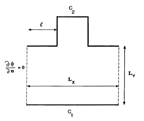
Figure 1: Schematic representation of the diffusion cell for the first fractal iteration of a fractal generator. The dimensions of the cell, ${L_{x}}=3l$ and ${L_{y}}=2l$, as well as the boundary conditions are indicated. For this fractal ${D_{F}}=\frac{{\log 5}}{{\log 3}}.$

We now focus on the case of mild diffusion. The purpose is to estimate the coefficients $A$ and $B$ analytically in this limit. To this end we follow the so-called ”independent field approximation” (IFA). This is a coarse-graining argument based on compartmentalization of the full continuous space in which diffusion takes place into a finite number of properly selected non-overlapping and non-interacting rectangular regions. Here, one can write down closed expressions for the entropy production and the variational functional assuming linear concentration profiles. The nonlinear dependence of the field in terms of the spatial coordinates arising from the irregularities of the boundaries is thus approximated by piecewise linear functions, entailing discontinuities of the equipotential lines at the boundaries between the cells.

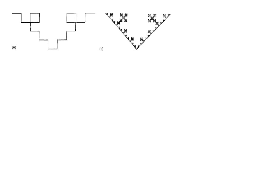
Figure 2: Shown are (a) the second and (b) the fourth fractal iterations of the fractal generator of Figure 1.

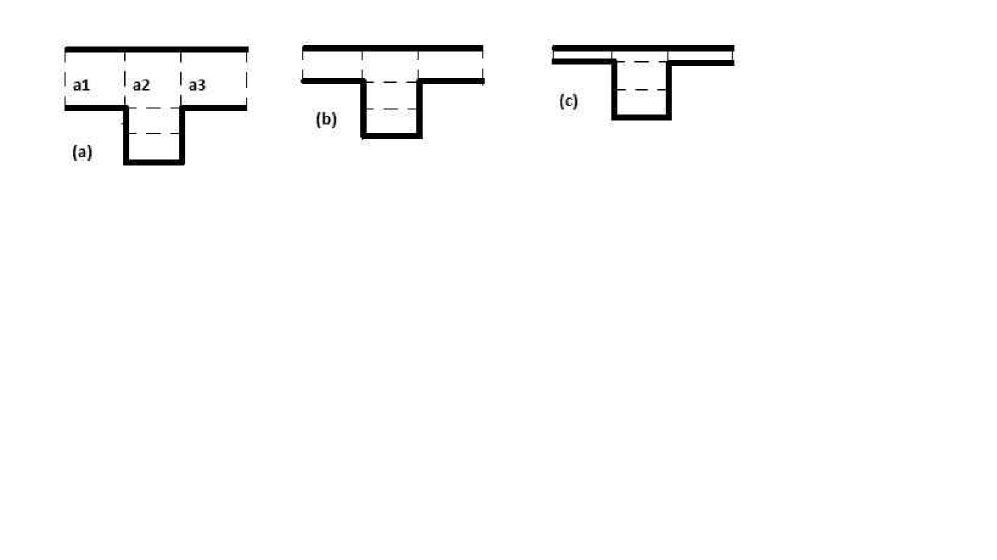
Figure 3: Schematic representation of the diffusion cell for the first fractal iteration of a fractal generator. The distance ${L_{y}}=ml$ (here $l=1$) is successively reduced from left to right: a) ${L_{y}}=m=0.3$ to b) ${L_{y}}=m=0.1$ and c) ${L_{y}}=m\to 0$.

Let us illustrate how the IFA works for the first few fractal generations of the cell. We separate the cell into the three rectangles shown in Figure 3. Accepting linear concentration profiles in each of the side parts ($a_{1}$) and ($a_{3}$) and applying eq.(5) with ${L_{x}}=l$, ${L_{y}}=ml$ (i.e. setting $F=Dk({c_{2}}-{c_{1}})\ln\frac{{{c_{2}}}}{{{c_{1}}}}$) one finds for the respective entropy production

$${P_{a_{1}}}={P_{a_{3}}}=\frac{F}{m}.$$ (9)

Assuming furthermore a linear half penetration inside the pore (that is, a linear concentration profile until the middle of the pore^19-20, thereby neglecting the remaining active zone) the central region ($a_{2}$) from eq.(5) with ${L_{x}}=l$ and ${L_{y}}=ml+\frac{l}{2}$ reads

$${P_{a_{2}}}=F\frac{l}{{ml+\frac{l}{2}}}=F\frac{2}{{2m+1}}.$$ (10)

Thus, the total entropy production of the cell becomes

$${P_{tot}}={P_{a_{1}}}+{P_{a_{2}}}+{P_{a_{3}}}=2F\frac{{3m+1}}{{m(2m+1)}}.$$ (11)

Applying now eqs.(5) and (6) for the whole cell with ${L_{x}}=3l$ and ${L_{y}}=ml$ we find (remember that we deal here with mild diffusion, see eq.(7)) that

$${P_{tot}}=\frac{{3FB(g)}}{m}.$$ (12)

So that, for the first iteration (Figure 1) the coefficient $B$ is of the form

$${B^{(1)}}=\frac{{6m+2}}{{3(2m+1)}}=\frac{2}{3}+\frac{2}{3}\frac{m}{{2m+1}}.$$ (13)

Similarly, for the second fractal iteration (Figure 2a) we obtain

$${B^{(2)}}=\frac{{324{m^{2}}+150m+12}}{{9(6m+1)(6m+3)}}=\frac{4}{9}+\frac{2}{3}m\left[{\frac{1}{{2m+1}}+\frac{2}{{1+6m}}}\right],$$ (14)

and for the third

$${B^{(3)}}=\frac{8}{{27}}+\frac{2}{3}m\left[{\frac{1}{{2m+1}}+\frac{2}{{6m+1}}+\frac{4}{{18m+1}}}\right],$$ (15)

where the superscript $(i)$ denotes the $i-th$ fractal iteration. Proceeding in the same lines one can find and prove by induction that for the $i-th$ fractal iteration it holds

$${B_{m}^{(i)}}={\left({\frac{2}{3}}\right)^{i}}+\left({\frac{2}{3}}\right)m\sum\limits_{k=1}^{i}{\frac{{{2^{k-1}}}}{{1+2\cdot{3^{k-1}}m}}}.$$ (16)

The superscript ($i$) denotes the corresponding fractal generation (i.e. $i=1$ is for the first fractal generation, $i=2$ is for the second etc) and $m$ indicates the respective inter-electrode distance.

Pausing for a moment the analysis of $B_{m}^{(i)}$, we investigate some features for the total entropy production of the fractal generations. Especially, one can easily observe that for the first few fractal iterations the total entropy production is

$$P_{tot}^{(1)}=2P_{a_{1}}^{(1)}+P_{a_{2}}^{(1)},~{}~{}P_{tot}^{(2)}=4P_{a_{1}}^{(2)}+2P_{a_{2}}^{(2)}+P_{a_{3}}^{(2)},$$ (17)

and

$$P_{tot}^{(3)}=8P_{a_{1}}^{(3)}+4P_{a_{2}}^{(3)}+2P_{a_{3}}^{(3)}+P_{a_{4}}^{(3)},~{}~{}P_{tot}^{(4)}=16P_{a_{1}}^{(4)}+8P_{a_{2}}^{(4)}+4P_{a_{3}}^{(4)}+2P_{a_{4}}^{(4)}+P_{a_{5}}^{(4)},$$ (18)

where the superscript ($i$) refers to the fractal iteration and the index $a_{i}$ corresponds to the geometrical structure that one can encounter in each fractal (see also Figure 3). For example, the index $a_{1}$ (or equivalently $a_{3}$) refers to the left (right) side part of the first fractal generation, while $a_{2}$ denotes the central region. Similarly, the indices $a_{4}$, $a_{5}$ refer to the central regions of the second and third fractal generations respectively etc. The above procedure implies that for the $i-th$ fractal iteration the total entropy production should be written as

$$P_{tot}^{(i)}={2^{i}}P_{a_{1}}^{(i)}+{2^{i-1}}P_{a_{2}}^{(i)}+{2^{i-2}}P_{a_{3}}^{(i)}+{2^{i-3}}P_{a_{4}}^{(i)}+...,$$ (19)

or in a more compact form

$$P_{tot}^{(i)}=\sum\limits_{k=0/i-k\geqslant 0}^{\infty}{{2^{i-k}}}P_{k}^{(i)}.$$ (20)

Here, the superscript ($i$) denotes the corresponding fractal generation (i.e. $i=1$ for the first fractal generation, $i=2$ for the second etc), whereas $k$ corresponds to each geometrical structure that appears in the corresponding fractal generation as explained above. Moreover, we can find that the entropy production for each geometrical structure can be written as

$$P_{a_{1}}^{(i)}=\frac{F}{{{3^{i-1}}m}}~{}~{}and~{}~{}P_{k}^{(i)}=\frac{{2F}}{{2\cdot{3^{i-k}}m+1}},k\geqslant 1,i\geqslant k,$$ (21)

while the above polynomials are connected through the recurrence relations

$$\begin{array}[]{*{20}{c}}{\frac{{P_{k+1}^{(l)}}}{{P_{k}^{(l)}}}=1+\frac{{4\cdot{3^{l}}m}}{{{3^{k+1}}+2\cdot{3^{l}}m}},}&{l\geqslant k,}&{k\geqslant 1}\end{array}~{}~{}and~{}~{}\begin{array}[]{*{20}{c}}{\frac{{P_{k}^{(l)}}}{{P_{a}^{(l)}}}=\frac{{2\cdot{3^{-1+l+k}}}}{{{3^{k}}+2\cdot{3^{l}}m}}}&{l\geqslant k,}&{k\geqslant 1}\end{array}.$$ (22)

Note also that the total entropy production for each fractal generation and geometrical structure can be written as

$$P_{tot}^{(i)}=F\frac{{{2^{i}}}}{{{3^{i-1}}m}}+2F\sum\limits_{k=1}^{i}{\frac{{{2^{k-1}}}}{{1+2\cdot{3^{k-1}}m}}}.$$ (23)

Coming back to the investigation of the coefficients $B_{m}^{(i)}$ we observe that the first derivative with respect to $m$ is positive

$$\frac{{\partial B_{m}^{(i)}}}{{\partial m}}=\frac{2}{3}\sum\limits_{k=1}^{i}{\frac{{{2^{k-1}}}}{{\left({2\cdot{3^{k-1}}+\frac{1}{m}}\right){m^{2}}}}},$$ (24)

implying that $B_{m}^{(i)}$ is an increasing function of $m$. We should also observe here that for m= 1, 2, 3 one finds again the results of³², (geometries for the Far field)

$$B_{1}^{(1)}=\frac{8}{9}\simeq 0.8889,B_{1}^{(2)}=\frac{6}{7}\simeq 0.8571,...,B_{1}^{(5)}=\frac{{245,451,914}}{{289,739,835}}\simeq 0.8471,$$ (25)

with a limiting value (in the context of the IFA approximation)

$$B_{1}^{(10)}=\frac{{22,614,533,817,495,831,212,892,038}}{{26,698,620,787,529,312,076,958,125}}\simeq 0.8470.$$ (26)

III Predictions for the Near Field

As also pointed out in the introduction, the ”Near Field” is a situation not studied before in the literature. Supposing that in the phenomenon there is no new physics, we can apply our real space renormalization scheme (IFA) in order to obtain predictions and compare them with the finite element predictions, considered here as reference values. More specifically, we can easily confirm that for $m=0.3$ the predictions of our real space renormalization scheme are

$$B_{0.3}^{(1)}=\frac{{19}}{{24}}\simeq 0.7916,B_{0.3}^{(2)}=\frac{{359}}{{504}}\simeq 0.7123,...,B_{0.3}^{(5)}=\frac{{6186317}}{{9069732}}\simeq 0.6821,$$ (27)

approaching asymptotically the value (in the framework of the IFA)

$$B_{0.3}^{(10)}=\frac{{2,574,446,468,051,339,779,667,687}}{{3,776,514,354,889,019,285,033,772}}\simeq 0.6817.$$ (28)

Similarly, for m=0.1 the predictions of the renormalization are

$$B_{0.1}^{(1)}=\frac{{13}}{{18}}\simeq 0.7222,B_{0.1}^{(2)}=\frac{7}{{12}}\simeq 0.5833,...,B_{0.1}^{(5)}=\frac{{37388}}{{73143}}\simeq 0.5112.$$ (29)

Giving a limiting value in the context of the IFA approximation

$$B_{0.1}^{(10)}=\frac{{16,308,004,933,962,338,624}}{{31,975,093,599,832,520,109}}\simeq 0.5100.$$ (30)

Quite curiously, the renormalization procedure gives also a finite limit when $m\to 0$, that is

$$B_{0.0}^{(1)}=\frac{2}{3}\approx 0.667,B_{0.0}^{(2)}=\frac{4}{9}\approx 0.444,B_{0.0}^{(3)}=\frac{8}{{27}}\approx 0.296,B_{0.0}^{(4)}=\frac{{16}}{{81}}\approx 0.198.$$ (31)

Thus, we can conclude that $B_{m=0}^{(i)}={\left({\frac{2}{3}}\right)^{i}}$, as it is expected from the Cantor structure of the counter membrane. Table I presents the values of $B_{m}^{(i)}$ predicted by the IFA for the first eight fractal iterations. It appears that $B_{m}^{(i)}$ take intermediate values of the order of 0.5 to 0.9. A monotonic decay is observed for successive prefractal generations as the distance $L_{y}=ml+l/2$ remains fixed. It is clear that when $L_{y}$ becomes very large ($L_{y}\to\infty$) $B_{m}$ tends to unity. As an empirical value coming now from our IFA approximation when $L_{y}=0.1$ the coefficient $B$ for the limiting fractal object approaches the value 0.51 (see Tables I,II). On the other hand, for a given fractal iteration as $L_{y}$ increases the corresponding values of $B$’s are increasing. Especially, it can be easily shown (through the IFA) that $\mathop{\lim}\limits_{m\to\infty}B_{m}^{(i)}={\left({\frac{2}{3}}\right)^{i}}+\frac{1}{3}{\sum\limits_{k=1}^{i}{\left({\frac{2}{3}}\right)}^{k-1}}$. From here, one can confirm that for large distances (i.e. $m\to\infty$ or equivalently $L_{y}\to\infty$) the limiting value of $B_{m}^{(i)}$ of every fractal iteration is equal to unity, as the spatial distribution of the concentration becomes roughly uniform for large distances ${L_{y}}$. Indeed, Table II shows the limiting value of the coefficients $B_{m}$ as the distance $L_{y}$ is increased. More specifically, we observe a monotonic increase for the limiting value from 0.5 to unity as $L_{y}$ becomes very large (of the order of ten, $L_{y}\sim 10$). As an illustration of the above discussion, Figure 4 depicts the evolution of the coefficients $B_{m}^{(i)}(g)$ (predicted through the IFA) with respect to different fractal iterations for various distances $m$ between the electrodes. In each case we observe a decay for increasing fractal iterations and a saturation of the corresponding coefficient (after the sixth fractal generation).

Table 1: In the table below, we present the values corresponding to the first few fractal generations of the coefficient $B_{m}^{(i)}(g)$ for different distances from the membrane. We clearly observe a saturation after the seventh fractal iteration. It is concluded that the limiting value of $B_{m}^{(f)}$ for the final fractal object is a function of the fractal dimension ${D_{f}}$ of the object.

Distance (m)	$B_{{m}}^{(1)}$	$B_{{m}}^{(2)}$	$B_{{m}}^{(3)}$	$B_{{m}}^{(4)}$	$B_{{m}}^{(5)}$	$B_{{m}}^{(6)}$	$B_{{m}}^{(7)}$	$B_{{m}}^{(8)}$
0.1	0.7222	0.5833	0.5304	0.5150	0.5112	0.5103	0.5101	0.5100
0.3	0.7917	0.7123	0.6892	0.6834	0.6821	0.6818	0.6817	0.6817
1.0	0.8889	0.8571	0.8493	0.8475	0.8471	0.8471	0.8470	0.8470
2.0	0.9333	0.9162	0.9122	0.9113	0.9111	0.9111	0.9111	0.9111
3.0	0.9524	0.9407	0.9380	0.9374	0.9373	0.9372	0.9372	0.9372

Table 2: The limiting value of the coefficient $B_{m}^{(i)}(g)$ predicted by the IFA is listed for various inter-electrode distances ($m$).

Distance ($m$)	Limiting value
0.1	0.5100
0.2	0.6178
0.3	0.6817
0.5	0.7584
0.7	0.8042
1.0	0.8470
2.0	0.9111
3.0	0.9372
10.0	0.9794

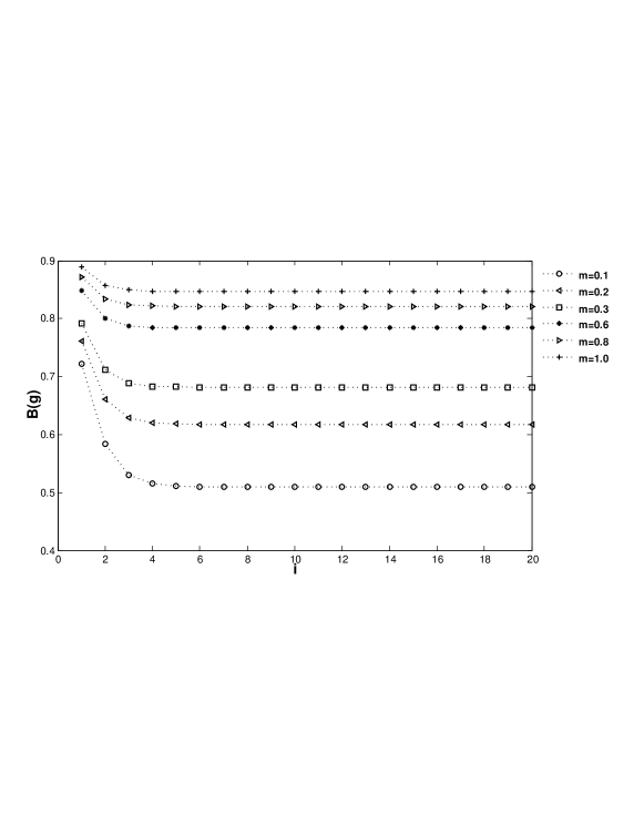
Figure 4: Shown are the coefficients $B(g)$ (eq.(16)) versus the fractal iteration $i$ for various inter-electrode ($m$) distances. We observe a saturation after the sixth fractal generation for a range of different distances.

IV Irregular Boundaries: Numerical Approach in the Near Field

The Laplace equation for geometries associated with the four first generations has been solved numerically using an in-house developed finite element code. All four geometries were discretized using six-noded triangular elements with quadratic shape functions with $C^{0}$ continuity at interelement boundaries. This resulted in a quadratic interpolation of the potential field and a linear variation of its gradient inside each element³⁴. The global entropy production was then computed for various boundary conditions by integrating the local entropy production obtained from the field and the associated flux (essentially its gradient) by means of relationship (2). This quadrature was implemented using a 25-integration points scheme derived by Laursen and Gellert³⁵. Dirichlet boundary conditions with constant concentrations $c_{1}$ and $c_{2}$ are imposed to the models. The meshes used for the calculations were produced using the GMSH meshing tool³⁶. A very fine discretization of the studied domain was intentionally selected in order to obtain sufficient precision on the values of the local entropy production and of the functional for the purpose of validation of the approximate coefficients. An element size on the order of 4.5 $10^{-3}$ for the points of the model was selected (for $L_{x}=1$) close to the fractal surface. The number of elements and nodes considered for each generation is reported in Table III (the min and max are related to the minimal and maximal distances between the electrodes).

Using the above method one may estimate the factor $B(g)$ with a very good precision (up to three significant digits). The numerical coefficients (obtained from the aforementioned numerical method) are presented in Tables IV-V while Table VI shows the comparison of the theoretical (IFA) and the corresponding numerical values for the coefficients $B_{{m}}^{(i)}$. These calculations indicate that the proposed approximate method is satisfactory for the first few fractal iterations and gets worse for increasing generation. Especially, Tables IV-V illustrate the validation of the phenomenological relation with the numerical evaluation via Finite Elements, arguably the central result of this paper. From a careful inspection of these Tables it is clear that as $L_{y}$ increases the coefficients $B_{m}^{(i)}$ increases as well which is at least in qualitative agreement with eq.(16) obtained by the IFA. We also observe a decrease of the coefficients $A$’s and $B$’s as the fractal generation increases. By inspecting Tables IV-V we observe that for $L_{y}\to 0.1$ a limiting value 0.65 is approached from the Finite Elements method while the value 0.51 is predicted by the IFA (see Table II). The latter indicates the failure of the IFA to be accurate at high fractal generations. However, a qualitative agreement between the IFA and the Finite Elements calculations is evident, which means that for the final fractal object the coefficients seem to tend to a limiting value independently of the concentration $c_{2}$. Commenting now on Table VI which presents the difference between the theoretical and numerical values (obtained with Finite Elements) of the coefficients $B_{m}^{(i)}$ for $c_{2}=0.9$, it is observed that as $L_{y}$ tends to zero substantial deviations from the corresponding theoretical value appear as a result of the divergence of the Laplacian field. Also, for increasing fractal iterations, we see from the Table VI that the relative error becomes important (see also below).

Table 3: The number of elements and nodes used for the numerical calculations (Finite Elements) for the first four fractal generations. The corresponding values are related to the minimal and maximal distances between the two electrodes.

Generation	Number of elements (min-max)	Number of nodes (min-max)
$1$	118953-318347	239450-638544
$2$	174147-385141	350578-772872
$3$	199691-408749	402816-821238
$4$	219401-428755	444236-863250

Table 4: The coefficients $B_{{m}}^{(i)ph}$ and $A_{{m}}^{(i)ph}$ (for the first four fractal generations) obtained from the respective numerical values of the variational functional $Q_{{m}}^{(i)ph}$ and the phenomenological entropy production $P_{{m}}^{(i)ph}$, with concentration ${c_{2}}=0.9$.

${L_{y}}$	${B^{(1)ph}}$	${B^{(2)ph}}$	${B^{(3)ph}}$	${B^{(4)ph}}$	${A^{(1)ph}}$	${A^{(2)ph}}$	${A^{(3)ph}}$	${A^{(4)ph}}$
$0.1$	0.7780	0.6883	0.6620	0.6543	0.7779	0.6881	0.6622	0.6546
$0.3$	08664	0.8276	0.8170	0.8134	0.8665	0.8276	0.8172	0.8134
$0.5$	0.9066	0.8833	0.8766	0.8733	0.9064	0.8827	0.8763	0.8732
$1.0$	0.9500	0.9366	0.9333	0.9300	0.9491	0.9364	0.9333	0.9301

Table 5: The coefficients $B_{{m_{i}}}^{(i)ph}$ and $A_{{m_{i}}}^{(i)ph}$ (for the first four fractal generations) obtained from the respective numerical values of the variational functional $Q_{{m_{i}}}^{(i)ph}$ and the entropy production $P_{{m_{i}}}^{(i)ph}$, with concentration ${c_{2}}=0.01$.

${L_{y}}$	${B^{(1)ph}}$	${B^{(2)ph}}$	${B^{(3)ph}}$	${B^{(4)ph}}$	${A^{(1)ph}}$	${A^{(2)ph}}$	${A^{(3)ph}}$	${A^{(4)ph}}$
$0.1$	0.7779	0.6882	0.6620	0.6544	0.7776	0.6874	0.6606	0.6520
$0.3$	0.8662	0.8280	0.8174	0.8139	0.8661	0.8277	0.8166	0.8128
$0.5$	0.9070	0.8829	0.8758	0.8734	0.9069	0.8827	0.8755	0.8728
$1.0$	0.9491	0.9361	0.9322	0.9308	0.9490	0.9360	0.9320	0.9306

Table 6: Percentage difference, with concentration ${c_{2}}=0.9$ and various distances $L_{y}$, between the two electrodes for the theoretical and the corresponding numerical values of the coefficients $B_{{m}}^{(i)}$.

${L_{y}}$	${B^{(1)}}$	${B^{(2)}}$	${B^{(3)}}$	${B^{(4)}}$
$0.1$	$7.2\%$	$15.2\%$	$19.9\%$	$21.3\%$
$0.3$	$8.6\%$	$13.9\%$	$15.7\%$	$15.9\%$
$0.5$	$8.1\%$	$11.9\%$	$12.9\%$	$13.0\%$
$1.0$	$6.4\%$	$8.5\%$	$9.0\%$	$8.9\%$

Another attempt to improve the above procedure is to insert the phenomenological (numerical) values for the coefficients $B_{m}^{(1)ph}$, and actually obtain a ”renormalized” value for the higher order coefficients e.g. $B_{m}^{(2)}$ etc, thus improving considerably the predictions of the theory. Combining the empirical result for the first generation with a IFA half penetration argument inside the new pores for the second fractal generation, one can find

$$B_{0.5}^{(2)ren}=\left({0.908-\frac{2}{3}}\right)3l+2\frac{8}{9}l=0.834,$$ (32)

while

$$B_{0.3}^{(2)ren}=0.786~{}~{}and~{}~{}B_{0.1}^{(2)ren}=0.639.$$ (33)

Comparing now the above results we can find that $B_{0.5}^{(2)ren}$ differs from $B_{0.5}^{(2)ph}$ by only $5.8\%$. Similarly $B_{0.3}^{(2)ren}$ differs from $B_{0.3}^{(2)ph}$ by only $5.7\%$ and $B_{0.1}^{(2)ren}$ differs from $B_{0.1}^{(2)ph}$ by $8.6\%$. In the same way, we can proceed with the remaining orders. Also, one can try various renormalization schemes together with the theoretical arguments. The best results are obtained when one uses for the prediction of the coefficient of the $k+1$ fractal iteration ${B^{(k+1)}}$ only the empirical coefficients of the previous $k$ iteration and no theoretical argument at all. For instance, for the case of the second fractal iteration for distance $m=0.5$ one can find

$$B_{0.5}^{{}^{(2)fren}}=\left({0.908-\frac{2}{3}}\right)3l+\frac{2}{3}0.949\simeq 0.8746,$$ (34)

where the superscript ”fren” stands for ”fully renormalized”. Here, the difference between $B_{0.5}^{{}^{(2)fren}}$ and $B_{0.3}^{(2)ph}$ is of the order of $1.2\%$. Figures 5-12 present the spatial dependence of the entropy production for the first four fractal iterations, for ${L_{y}}=0.3$, for the cases of strong (${c_{2}}=0.1$) and mild (${c_{2}}=0.9$) diffusion respectively. We observe that the behaviour of the local entropy production depends strongly from $c_{2}$. In particular, for the case of strong diffusion (see Figures 5,7,9,11) the appearance of a passive zone is observed irrespectively of the fractal generation. In contrast, for the case of mild diffusion the above statement breaks down, being indicated by the spreading of the local entropy production near the geometrical irregularities (see Figures 6,8,10,12).

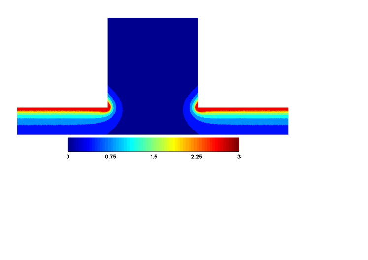
Figure 5: Spatial dependence of the entropy production for the diffusion cell of Figure 1. It is shown the case of strong diffusion with ${c_{2}}=0.1$, while the distance between the electrodes is ${L_{y}}=0.3$. (Computer units.)

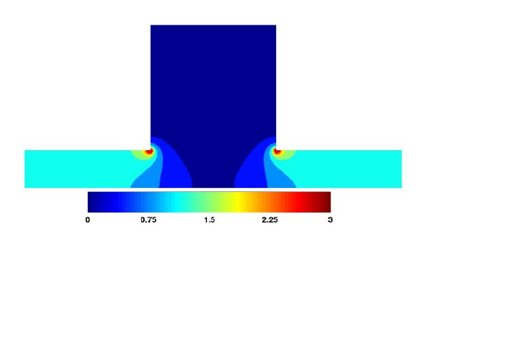
Figure 6: Spatial dependence of the entropy production for the diffusion cell of Figure 1. It is shown the case of mild diffusion with ${c_{2}}=0.9$, while the distance between the electrodes is ${L_{y}}=0.3$. (Computer units.)

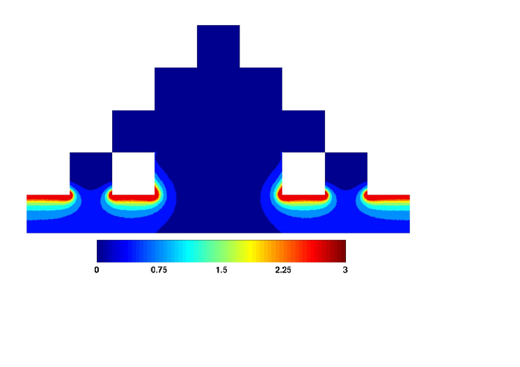
Figure 7: Spatial dependence of the entropy production for the second fractal iteration. It is shown the case of strong diffusion with ${c_{2}}=0.1$, while the distance between the electrodes is ${L_{y}}=0.3$. (Computer units.)

Let us briefly recall here the argument which relates the coefficients $A$ and $B$ through the active zone concept for the case of mild diffusion, i.e. $\left|{({c_{2}}-{c_{1}})/{c_{1}}}\right|=O(\varepsilon)$, $\varepsilon\ll 1$, with ${c_{1}}=O(1)$. Here, from eqs (7) and (8) one can conclude that $P\approx{\varepsilon^{2}}$ and $Q\approx{\varepsilon^{2}}$ while $B(g)\approx\mathop{\lim}\limits_{{c_{2}}\to{c_{1}}}{A^{mild}}({c_{1}},{c_{2}};g)$ up to a factor of $Dk/{c_{1}}$. The basic idea of this argument is that the profiles of the concentrations are essentially linear in space in the whole active volume and the nonlinearities are smoothly approximated.

In the opposite situation, we have the strong diffusion. One particular case of strong diffusion, which we study here in detail, is the case of the harmonic measure (${c_{1}}=1$, ${c_{2}}\to 0$).

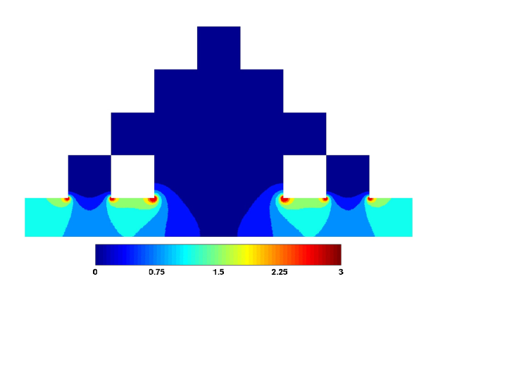
Figure 8: Spatial dependence of the entropy production for the second fractal iteration. It is shown the case of mild diffusion with ${c_{2}}=0.9$, while the distance between the electrodes is ${L_{y}}=0.3$. (Computer units.)

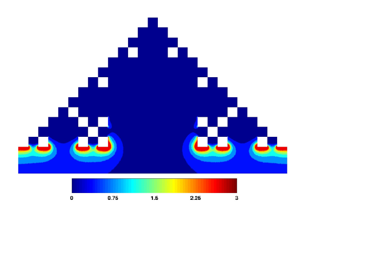
Figure 9: Spatial dependence of the entropy production for the third fractal generation. It is shown the case of strong diffusion with ${c_{2}}=0.1$, while the distance between the electrodes is ${L_{y}}=0.3$. (Computer units.)

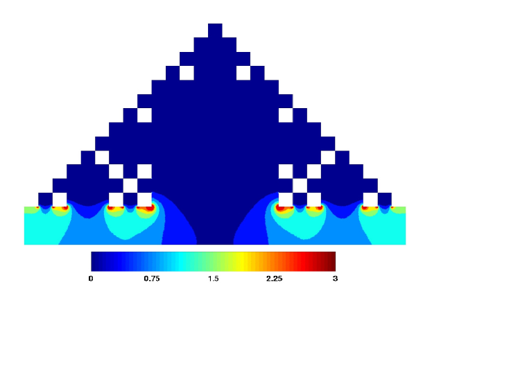
Figure 10: Spatial dependence of the entropy production for the third fractal generation. It is shown the case of mild diffusion with ${c_{2}}=0.9$, while the distance between the electrodes is ${L_{y}}=0.3$. (Computer units.)

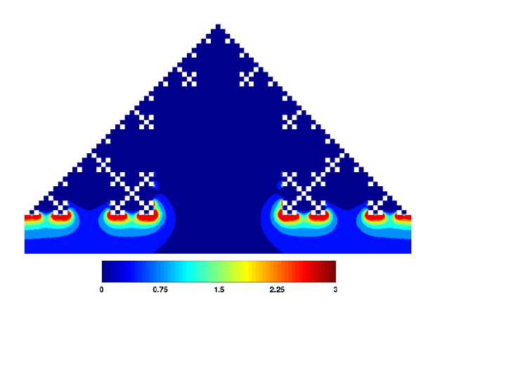
Figure 11: Spatial dependence of the entropy production for the fourth fractal generation. It is shown the case of strong diffusion with ${c_{2}}=0.1$, while the distance between the electrodes is ${L_{y}}=0.3$. (Computer units.)

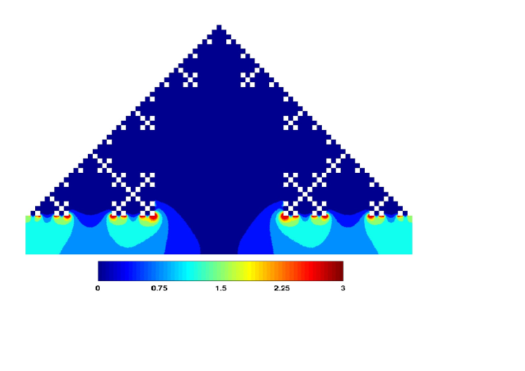
Figure 12: Spatial dependence of the entropy production for the fourth fractal generation. It is shown the case of mild diffusion with ${c_{2}}=0.9$ and distance between the electrodes ${L_{y}}=0.3$. (Computer units.)

Exactly in this case we obtain a visual interpretation of Makarov’s theorem. The measure is spreading on the surface of the working membrane almost uniformly in a length which roughly coincides with the diameter of the active membrane $l+\frac{l}{2}+\frac{l}{2}+l=3l$. In this case, Makarov’s theorem guarantees that at least for ${c_{2}}>0.01$, $A=B$ holds (see also Tables IV-V). We thus obtain a very important result of our real space renormalization scheme: Estimating the values of $B(g)$ with the active zone approximation (Mandelbrot’s argument) we obtain also the value of $A$ in the whole range of ${c_{2}}$, that is in all cases except from the case where ${c_{2}}<0.01$.

The above remarks indicate that the aforementioned IFA scheme is valid (in the Far and Near domain) at least for the first few fractal iterations for both strong and mild diffusion. Indeed, it is remarkable that such a simple renormalization scheme gives accurate predictions for the first fractal generations and leads at least to qualitative results for higher iterations (here up to the fourth). From our numerical calculations it turns out that the quality of the IFA prediction gets worse as the fractal generation increases and/or as the inter-electrode distance tends to zero (see Table VI). The basic reason behind this result is that the IFA is a coarse-graining approximation which neglects the fine microscopic details of the fractal objects. This is exactly the way to the passive zone approximation. Thus, it is a challenging open question whether the above conclusions can be straightforwardly generalized for even higher fractal iterations, where the IFA approximation is expected to fail. This constitutes a heavy computational task especially for high enough fractals iterations. In particular, three questions remain to be checked: a) to what extent the fully renormalized scheme is valid for higher fractal iterations, b) whether the limiting value predicted by the IFA approximation holds as a qualitative argument and c) the investigation of a better renormalization scheme that takes into account the respective correlations in the distribution of the harmonic measure especially for $m\rightarrow 0$.

V Conclusions and Discussion

The transport associated to molecular transfer of neutral particles from a diffusional field to an irregular membrane is examined from the standpoint of irreversible thermodynamics. Combining non-equilibrium thermodynamics and an argument developed initially by Mandelbrot et al.¹⁹, and then by Makarov et al.^28,29, one is led to probe and predict the entropy production and the variational functional of the transfer. Detailed predictions are given for the whole range of distances from the Far field to the Near field corroborated by finite differences^2,32,33 and Finite Elements calculations.

The central idea of the active zone concept² is that on the grounds of the Laplacian transfer on a membrane, certain parts of the membrane remain passive and all thermodynamic properties of the membrane can be estimated with a very good approximation by the contribution of the ”active parts”. In the context of the active zone introduced by spectroscopic impedance, a system with irregular boundaries possesses, in the Makarov regime where the reactive system is ”almost entirely diffusive”, the same impedance as a smaller system with regular boundary conditions. This ${L_{app.Mak}}$ ”apparent, spectroscopic length”, is not the same as the quantity ${L_{app,entr}}=B(g){L_{x}}$ but the conclusion remains the same: an entirely diffusive system with irregular boundary conditions possesses the same entropy production as a system with smaller diameter and regular (flat) boundary conditions. This can be seen as an interpretation of Makarov’s theorem in terms of irreversible thermodynamics. Do these remarks apply to the ”Near field” ? In the Near field the original Mandelbrot’s argument boils down and the notion of spectroscopic impedance is relaxed. However, as it is shown here one does not expect ”new physics” and irreversible thermodynamics is still valid. Our remarks, are corroborated from the evaluation of the local entropy production around the von Koch curve in the Near field.

To be concrete, the entropy production and the variational functional of Laplacian transfer for geometries associated with the first few fractal iterations leading eventually to a fractal generator (von Koch curve) are studied. We first recover and recapitulate results for the Far field. Then, we turn to the case of the ”Near field”, a situation not studied before in the literature, for both strong and mild diffusion. Detailed charts of the local entropy production around the first four iterations are given, and the global entropy production is investigated carefully. From these studies it is clear that the Laplacian fields are in a sense a ”smooth measure” around irregular objects. Moreover, the analytic procedure which allows one to approximate the entropy production seems to be quite powerful and straightforward. Although the spatial distribution of the local entropy production changes greatly from the mild to strong diffusion, the IFA analysis and the global entropy production obey the same rules in the Far and in the Near field. A fair evaluation of the IFA arguments implies that the difference between the predicted and the numerically obtained values increases with the fractal iterations. An interpretation of the above statement is that the IFA is a coarse-graining approximation which neglects the fine microscopic details of the fractal objects (passive zone approximation). More specifically, in the framework of our IFA renormalized $B$’s for the first three generations differ by $5-15\%$ from the numerical reference values, and the fully renormalized B’s coincide up to $2\%$ difference to the numerical values. As already pointed out, the generalization of these results for higher fractal iterations constitutes an interesting open problem. Another question that arises from our investigation is whether the predicted by the IFA limiting value of the coefficient $B$ for high fractal generations holds at least qualitatively. This task requires heavy computations for the Laplacian transfer of high fractal objects and has to be performed in the context of a supercomputer. Finally, as we have also mentioned in the past, our predictions on such dissipation trends should be amenable to experimental testing in a suitably constructed diffusion cell.

References

- (1) M. Filoche and B. Sapoval, Transfer across random versus deterministic fractal interfaces, Phys. Rev. Lett. 84(25) (2000) 5776.
- (2) B. Sapoval, M. Filoche, K. Karamanos and R. Brizzi, Can one hear the shape of an electrode I. Numerical study of the active zone in Laplacian transfer, Eur. Phys. J. B-Condensed Matter and Complex Systems 9(4) (1999) 739-753.
- (3) J. Bourgain, On the Hausdorff dimension of harmonic measure in higher dimension, Inventiones Mathematicae 87(3) (1987) 477-483.
- (4) C. F. Gerald and P. O. Wheatly, Applied Numerical Analysis, 4th Ed. (Addison-Wesley, Reading, MA, 1989).
- (5) B. B. Mandelbrot, The Fractal Geometry of Nature, (Freeman, San Francisco, 1982).
- (6) B. Sapoval, Universalites et Fractales, (Flammarion, Paris, 1997).
- (7) T. Vicsek, Fractal Growth Phenomena, (World Scientific, Singapore, 1989).
- (8) E. R. Weibel, The Pathway for Oxygen, (Harvard University Press, Cambridge, MA, 1984).
- (9) B. J. West, Physiology in fractal dimensions: error tolerance, Ann. Biomed. Eng. 18 (1990) 135.
- (10) B. J. West and W. Deering, Fractal physiology for physicists: Levy statistics, Phys. Rep. 246(1) (1994) 1-100.
- (11) B. J. West, V. A. L. M. I. K. Bhargava and A. L. Goldberger, Beyond the principle of similitude: renormalization in the bronchial tree, Journal of Applied Physiology 60(3) (1986) 1089-1097.
- (12) G. B. West, J. H. Brown and B. J. Enquist, A general model for the origin of allometric scaling laws in biology, Science 276(5309) (1997) 122-126.
- (13) D. S. Grebenkov, What makes a boundary less accessible, Phys. Rev. Lett. 95(20) (2005) 200602.
- (14) D. S. Grebenkov, Scaling properties of the spread harmonic measures, Fractals 14(03) (2006) 231-243.
- (15) A. Hill, Entropy production as the selection rule between different growth morphologies, Nature (London) 348 (1990) 426-428.
- (16) K. Karamanos, Dissipation in weakly polarizable electrodes across irregular boundaries, J. Noneq. Therm. 30(2) (2005) 163-171.
- (17) J. Lefevre, Is there a relationship between fractal complexity and functional efficiency in the pulmonary arterial tree? J. Physiol. 446 (1992) 578.
- (18) S. H. Liu, Fractal model for the ac response of a rough interface, Phys. Rev. Lett. 55(5) (1985) 529.
- (19) C. J. G. Evertsz and B. B. Mandelbrot, Harmonic measure around a linearly self-similar tree, J. Phys. A 25(7) (1991) 1781.
- (20) R. Gutfraind and B. Sapoval, Active surface and adaptability of fractal membranes and electrodes, J. Phys. I 3(8) (1993) 1801-1818.
- (21) P. Meakin and B. Sapoval, Random-walk simulation of the response of irregular or fractal interfaces and membranes, Phys. Rev. A 43(6) (1991) 2993.
- (22) H. Ruiz-Estrada, R. Blender and W. Dieterich, AC response of fractal metal-electrolyte interfaces, J. Phys - Cond. Matter. 6(48) (1994) 10509.
- (23) B. Sapoval, R. Gutfraind, P. Meakin, M. Keddam and H. Takenouti, Equivalent-circuit, scaling, random-walk simulation, and an experimental study of self-similar fractal electrodes and interfaces, Phys. Rev. E 48(5) (1993) 3333–3344.
- (24) J. Crank, The Mathematics of Diffusion, 2nd ed. (Clarendon, Oxford, 1975).
- (25) B. Duplantier, Harmonic Measure Exponents for Two-Dimensional Percolation, Phys. Rev. Lett. 82(20) (1999) 3940–3943.
- (26) B. Duplantier, Path-crossing exponents and the external perimeter in 2D percolation, Phys. Rev. Lett. 83(7) (1999) 1359–1362.
- (27) B. Duplantier, Conformally Invariant Fractals and Potential Theory, Phys. Rev. Lett. 84(7) (2000) 1363–1367.
- (28) P. Jones and T. Wolff, Hausdorff dimension of harmonic measure in the plane, Acta Math. 161(1) 131-144 (1998).
- (29) N. G. Makarov, On the distortion of boundary sets under conformal mappings, Proc. London Math. Soc. 3(2) (1985) 369-384.
- (30) M. Rosso, Y. Huttel, E. Chassaing, B. Sapoval and R. Gutfraind, Visualization of the active zone of an irregular electrode by optical absorption, J. Electrochem. Soc. 144(5) (1997) 1713.
- (31) D. Grebenkov, A. Lebedev, M. Filoche and B. Sapoval, Multifractal properties of the harmonic measure on Koch boundaries in two and three dimensions, Phys. Rev. E 71(5) (2005) 056121.
- (32) K. Karamanos, G. Nicolis, T. Massart and P. Bouillard, Dissipation in Laplacian fields across irregular boundaries, Phys. Rev. E 64(1) (2001) 0111151–15.
- (33) K. Karamanos, Recycling the Independent Field Approximation Argument in the Far Field, AIP Conf. Proc. 1303(1) (2010) 45–51.
- (34) O. C. Zienciewicz, The Finite Elements Method, 5th ed. (McGraw - Hill, UK, 2000).
- (35) M. E. Laursen and M. Gellert, Some criteria for numerically integrated matrices and quadrature formulas for triangles, Int. J. Numer. Methods Eng. 12(67) (1978).
- (36) C. Geuzaine and JF. Remacle, Gmsh: A 3-D finite element mesh generator with built-in pre-and post-processing facilities, Int. J. Numer. Meth. Eng. 79(11) (2009) 1309-1331.