Stability and phase transition of localized modes in Bose-Einstein condensates with both two- and three-body interactions

Abstract

We investigate the stability and phase transition of localized modes in Bose-Einstein Condensates (BECs) in an optical lattice with the discrete nonlinear Schrödinger model by considering both two- and three-body interactions. We find that there are three types of localized modes, bright discrete breather (DB), discrete kink (DK), and multi-breather (MUB). Moreover, both two- and three-body on-site repulsive interactions can stabilize DB, while on-site attractive three-body interactions destabilize it. There is a critical value for the three-body interaction with which both DK and MUB become the most stable ones. We give analytically the energy thresholds for the destabilization of localized states and find that they are unstable (stable) when the total energy of the system is higher (lower) than the thresholds. The stability and dynamics characters of DB and MUB are general for extended lattice systems. Our result is useful for the blocking, filtering, and transfer of the norm in nonlinear lattices for BECs with both two- and three-body interactions.

I Introduction

Localized excitation in Bose-Einstein condensates (BECs) has become one of the most interesting topics in nonlinear lattice systems since the discrete breathers (DBs) and the intrinsic localized modes are discovered YIshimori1982 ; MPeyrard1984 ; Sievers1988 . The most well-known fascinating feature of the localized mode is that it can propagate without changing its shape as a result of the balance between nonlinearity and dispersion DKCampbell2004 ; Campbell2004 ; SFlach2008 ; HHennig2013 . DB arises intrinsically from the interplay between the nonlinearity and the discreteness of the system. DB has been observed in various systems, such as micromechanical cantilever arrays MSato2006 , antiferromagnet systems UTSchwarz1999 ; MSato2004 , Josephson-junction arrays ETrias2000 ; AVUstinov2003 , nonlinear waveguide arrays RMorandotti1999 ; HSEisenberg1998 , BECs BEiermann2004 ; ATrombettoni2001 , Tonks gas Kolomeisky1992 , superfluid fermi gases JuKuiXue2008 , and some dissipative systems MGClerc2011 ; PCMatthews2011 . The static, dynamical, and other properties of DB have been studied theoretically in the last decade SAubry1997 ; JDorignac2004 ; HSakaguchi2010 ; MMatuszewski2005 ; NBoechler2010 . It has been demonstrated that DBs are attractors in dissipative systems SFlach1998 ; PJMartinez2003 ; RSMacKay1998 , or act as virtual bottlenecks which slow down the relaxation processes in generic nonlinear lattices GPTsironis1996 ; RLivi2006 ; GSNg2009 . It is shown that the stability of the discrete localized modes plays a crucial role in blocking, filtering, and transfer of the norm through a localized mode. By far, there are many interesting works focused on this stability by considering two-body interactions HHennig2010 ; RFranzosi2011 ; LuLi2005 ; ZXLiang2005 ; yingwu2004 ; XDBai2012 .

Recently, the three-body interactions could be observed or realized in experiment and theory SWill2010 ; DaleyAJ2014 . In 2014, Petrov WSBakr2014 proposed a method to control the two- and three-body interactions in ultracold Bose gas in any dimension. The three-body interactions play an important role in many interesting physical phenomena TLuu2007 ; BolunChen2008 ; PRJohnson2009 ; KezhaoZhou2010 , and even lead to a variety of unique properties that are absent in the system dominated by the two-body interactions which can be governed by a Feshbach resonance SInouye1998 . For example, in 2010, Dasgupta RDasgupta2010 discovered that if the two-body interactions are attractive, the presence of three-body interactions makes the crossover process from Bardeen-Cooper-Schrieffer (BCS) to Bose-Einstein condensates (BECs) a nonreversible one. In 2012, Singh et al. MSingh2012 found that the coupling of the two- and three-body interactions can affect strongly the transition from Mott insulator to superfluid for ultracold bosonic atoms in an optical lattice or a superlattice. Up to now, there are few works on localized excitations in nonlinear lattice systems by considering three-body interactions. Especially, there are no systematical analysis of the types, existence, and stability of the localized modes, such as DB, the discrete kink (DK) PGKevrekidis2002 ; YuAKosevich2004 ; JMSpeight1999 , and multi-breather (MUB). It is natural to ask how the two- and three-body interactions affect these properties of the localized modes in BECs.

In this paper, we investigate the stability and phase transition of localized modes in BECs in an optical lattice with a discrete nonlinear Schrödinger model (DNLS) in the case by considering both two- and three-body interactions. We find that there are three different types of localized modes, that is, DB, DK, and MUB, and give the critical conditions for these localized modes. Both the two- and three-body on-site repulsive interactions can stabilize DB, while the three-body on-site attractive interactions destabilize it. We calculate analytically the energy thresholds, the Peierls-Nabarro (PN) energy barrier YSKivshar1993 ; BRumpf2004 , characterizing the stability of the localized excitation modes. If the total energy of the system is higher (lower) than the thresholds, the localized states are unstable (stable). Moreover, the stability and dynamics characters of DB and MUB are general for extended lattice systems. Our result is important for the transfer of BECs through the discrete localized modes, and is useful for controlling the transmission of matter waves in interferometry and quantum-information processes when there are both two- and three-body interactions in the system.

II localized states and Peierls-Nabarro barrier

II.1 The model

Besides the on-site two-body interactions, let us investigate the effect on transfer of BECs through discrete localized mode from the on-site three-body interactions of ultracold Bose gas in an optical lattice. Under the mean-field theory, the Hamiltonian of the system of BECs in an optical lattice can be written as AXZhang2008 :

$$\!\mathcal{H}\!\!=\!\!\sum_{n=1}^{M}\!\frac{U_{1}}{2}|\psi_{n}|^{4}\!+\!\sum_{n=1}^{M}\!\frac{U_{2}}{3}|\psi_{n}|^{6}\!-\!\frac{J}{2}\!\sum_{n=1}^{M-1}\!\left(\psi_{n}^{*}\psi_{n+1}\!+c.c\right).$$ (1)

Here $n$ $(=1,\cdots,M)$ is the index of the site. $\psi_{n}$ is a complex variable and $|\psi_{n}(t)|^{2}\equiv N_{n}(t)$ is the mean number of bosons at site $n$ (i.e., the norm $N_{n}(t)$). The first two terms represent the mean-field two- and three-body interaction energy, respectively, and the third term describes the hopping between nearest-neighboring sites. $U_{1}=4\pi\hbar^{2}a_{s}V_{eff}/m$ represents the effective on-site inter-atomic two-body interaction, where $V_{eff}$ is the effective mode volume of each site, $m$ is the atomic mass, and $a_{s}$ is the s-wave atomic scattering length. Here, we focus on the repulsive two-body interaction, i.e., $U_{1}>0$. $U_{2}$ represents the effective on-site inter-atomic three-body interactions, including both the repulsive and the attractive three-body interactions which are represented by $U_{2}>0$ and $U_{2}<0$, respectively. $J$ is the tunneling amplitude. Within the canonical equation $i\frac{\partial\psi_{n}}{\partial\tau}=\frac{\partial H}{\partial\psi_{n}^{*}}$, one can obtain the dimensionless DNLS AXZhang2008 ; BBBaizakov2009 ; EWamba2011

$$\!i\frac{\partial\psi_{n}}{\partial t}\!=\!\lambda_{1}\left|\psi_{n}\right|{}^{2}\psi_{n}\!+\!\lambda_{2}\left|\psi_{n}\right|{}^{4}\psi_{n}\!-\!\frac{1}{2}\left[\psi_{n-1}\!+\psi_{n+1}\right],$$ (2)

where

$$\sum_{n=1}^{M}|\psi_{n}|^{2}=1.$$ (3)

Here, $\lambda_{1}=U_{1}/J$, $\lambda_{2}=U_{2}/J$ and $t=J\tau$ are the normalized dimensionless two-body interaction, three-body interaction and time, respectively. Assume that $\psi_{n}(t)=A_{n}(t)\text{exp}\left(\text{$i\theta$}_{n}(t)\right)$, the Hamiltonian $H$ becomes

$$H\!=\!\!\sum_{n=1}^{M}\!\!\left(\frac{\lambda_{1}}{2}A_{n}^{4}\!+\!\frac{\lambda_{2}}{3}A_{n}^{6}\right)\!\!-\!\!\!\sum_{n=1}^{M-1}\!\!\left[A_{n}A_{n+1}\!\cos(\theta_{n}\!\!-\!\theta_{n+1})\right].$$ (4)

Usually, we use the Peierls-Nabarro (PN) energy landscape YSKivshar1993 ; BRumpf2004 to reflect the fact that discreteness breaks the continuous translational invariance of a continuum model. It is related to the PN potential whose amplitude can be seen as the minimum barrier which should be overcome to translate an object by one site. As in Ref. HHennig2010 , the PN energy landscape is defined as follows: for a given configuration of amplitudes $A_{n}$, with respect to the phase difference $\delta\theta_{ij}=\theta_{i}-\theta_{j}$, the PN energy landscape is obtained by extremizing $H$

$$H_{\text{PN}}^{l}=\underset{\delta\theta_{ij}}{\min}(-H),\;\;\;\;\;\;\;\;\text{ }H_{\text{PN}}^{u}=\underset{\delta\theta_{ij}}{\max}(-H),$$ (5)

where $H_{\text{PN}}^{l}$ and $H_{\text{PN}}^{u}$ are the lower and upper parts of the PN landscape, respectively.

In order to give an insight into the dynamical behavior of BECs in an optical lattice with both two- and three-body interactions, we mainly consider the nonlinear trimer model, i.e., the DNLS with $M=3$ lattice sites. In this case, the Hamiltonian $H$ of the system is

$$\!\!\!\!\!\!H_{M=3}\!\! \!=\! \!\!\frac{\lambda_{1}}{2}\left(A_{1}^{4}+A_{2}^{4}+A_{3}^{4}\right)+\frac{\lambda_{2}}{3}\left(A_{1}^{6}+A_{2}^{6}+A_{3}^{6}\right)$$ (6)

$$-\left[A_{1}A_{2}\cos\left(\theta_{1}\!\!-\theta_{2}\right)\!+\!A_{2}A_{3}\cos\left(\theta_{2}\!\!-\theta_{3}\right)\right],$$

where $\delta\theta_{12},\delta\theta_{23}\in[0,\pi]$. When $\delta\theta_{12}=\delta\theta_{23}=0$, one can get the upper PN energy landscape

$$H_{\text{PN}}^{u}\!\! = \!\!-\frac{\lambda_{1}}{2}\left(A_{1}^{4}+A_{2}^{4}+A_{3}^{4}\right)-\frac{\lambda_{2}}{3}\left(A_{1}^{6}+A_{2}^{6}+A_{3}^{6}\right)\;\;\;\;$$ (7)

$$+\left(A_{1}+A_{3}\right)A_{2}.$$

When $\delta\theta_{12}=\delta\theta_{23}=\pi$, the lower PN energy landscape can be obtained as

$$H_{\text{PN}}^{l}\!\! = \!\!-\frac{\lambda_{1}}{2}\left(A_{1}^{4}+A_{2}^{4}+A_{3}^{4}\right)-\frac{\lambda_{2}}{3}\left(A_{1}^{6}+A_{2}^{6}+A_{3}^{6}\right)\;\;\;\;$$ (8)

$$-\left(A_{1}+A_{3}\right)A_{2}.$$

The lower and the upper parts of the PN landscape bound the phase space of the trimer HHennig2010 . Because the localized mode whose properties we are studying corresponds to the minimum on $H_{\text{PN}}^{l}$, we should focus on the lower PN landscape, i.e., $\delta\theta_{12}=\delta\theta_{23}=\pi$.

II.2 Phase transition of localized states and Peierls-Nabarro barrier

To investigate the type of localized modes and its stability when the norm transfers through a localized mode, we use the nonlinear trimer model ($M=3$ for Eq.(2))

$$\begin{split}i\partial_{t}\psi_{1}&=\lambda_{1}\left|\psi_{1}\right|{}^{2}\psi_{1}+\lambda_{2}\left|\psi_{1}\right|{}^{4}\psi_{1}-\frac{1}{2}\psi_{2},\\ i\partial_{t}\psi_{2}&=\lambda_{1}\left|\psi_{2}\right|{}^{2}\psi_{2}+\lambda_{2}\left|\psi_{2}\right|{}^{4}\psi_{2}-\frac{1}{2}\left(\psi_{1}+\psi_{3}\right),\\ i\partial_{t}\psi_{3}&=\lambda_{1}\left|\psi_{3}\right|{}^{2}\psi_{3}+\lambda_{2}\left|\psi_{3}\right|{}^{4}\psi_{3}-\frac{1}{2}\psi_{2}.\end{split}$$ (9)

Here, the normalization reads $N=\sum_{n=1}^{3}\left|\psi_{n}\right|{}^{2}=1$. By setting $\delta\theta_{12}=\delta\theta_{23}=\pi$, from Eq. (9) one can get

$$\begin{split}&2\lambda_{1}A_{1}\left(1-2A_{1}^{2}-A_{3}^{2}\right)+2\lambda_{2}A_{1}\left(1-A_{3}^{2}\right)\!\!\left(1-2A_{1}^{2}-A_{3}^{2}\right)\\ &-\sqrt{1-A_{1}^{2}-A_{3}^{2}}+\frac{A_{1}\left(A_{1}+A_{3}\right)}{\sqrt{1-A_{1}^{2}-A_{3}^{2}}}=0,\\ &2\lambda_{1}A_{3}\left(1-2A_{3}^{2}-A_{1}^{2}\right)+2\lambda_{2}A_{3}\left(1-A_{1}^{2}\right)\!\!\left(1-2A_{3}^{2}-A_{1}^{2}\right)\\ &-\sqrt{1-A_{1}^{2}-A_{3}^{2}}+\frac{A_{3}\left(A_{1}+A_{3}\right)}{\sqrt{1-A_{1}^{2}-A_{3}^{2}}}=0.\end{split}$$ (10)

Let us define

$$\frac{\partial^{2}H_{\text{PN}}^{l}}{\partial A_{1}^{2}}\equiv H_{1},\;\;\;\;\frac{\partial^{2}H_{\text{PN}}^{l}}{\partial A_{1}\partial A_{3}}\equiv H_{2},\;\;\;\;\frac{\partial^{2}H_{\text{PN}}^{l}}{\partial A_{3}^{2}}\equiv H_{3},\;\;$$ (11)

and give inequality

$$H_{2}^{2}-H_{1}H_{3}\geq 0.$$ (12)

By solving Eq. (10) one can get the different kinds of solutions, including the stationary states and the saddle points. By substituting the saddle points obtained from Eq. (10) into Eq. (12), one can get the critical conditions which are the boundaries between phases I-III in Fig. 1. Actually, the boundaries can also be gained numerically from Eq. (10).

The results show that phase I occurs when $\lambda_{1}$ and $\lambda_{2}$ satisfy the relation

$$\lambda_{2}>1.68708-1.08801\lambda_{1}+0.00522\lambda_{1}^{2}.$$ (13)

For this case the norm can be pinned in any one of the three sites, shown in Fig. 2(a)-(c). There exists DB. That is, the norm is pinned in the middle site.

Phase III appears when $\lambda_{1}>3.5$ and $\lambda_{1}$ and $\lambda_{2}$ satisfy the relation

$$\begin{split}\lambda_{l}<\lambda_{2}<\lambda_{u},\end{split}$$ (14)

where

$$\begin{split}\lambda_{l}&=7.39452-4.33978\lambda_{1}+0.37649\lambda_{1}^{2}-0.0178\lambda_{1}^{3},\;\;\;\;\;\\ \lambda_{u}&=-12.223+6.6531\lambda_{1}-1.722\lambda_{1}^{2}+0.1715\lambda_{1}^{3}.\end{split}$$ (15)

In this case, the norms are localized in the adjacent two sites, shown in Fig. 2(e)-(g). It is called as DK.

Phase II is the part other than phases I and III, shown in Fig. 1. For this case, the norms of the three sites are nearly equivalent and there is no saddle point on the contour plots of the lower PN energy landscape $H_{PN}^{l}$, shown in Fig. 2(d) and (h). In this case, no localized mode exists.

To investigate the stability of the localized states, we pay our attention to the PN barrier. As shown in Fig. 2, the projection of $H_{PN}^{l}$ onto the $A_{1}-A_{3}$ plane exhibits one, two, or three minima. Each minimum refers to a stationary state. If there exist saddle points, the localized mode appears and these stationary states correspond to DB or DK. It is clear that the existence of DB, DK, and saddle points depends strongly on $\lambda_{1}$ and $\lambda_{2}$. We define the energy of DB (DK) as $E_{DB}$ ($E_{DK}$), the energy of the saddle points as $E_{thr}$, and the energy difference $\Delta E=E_{thr}-E_{DB(DK)}$. Actually, $\Delta E$ is the PN barrier. When the total energy of the trimer $E_{t}=-H>E_{thr}$ or $E_{t}-E_{DB(DK)}>E_{thr}-E_{DB(DK)}=\Delta E$, the DB (DK) should be unstable. On the contrary, when $E_{t}-E_{DB(DK)}<\Delta E$, the DB (DK) should be stable. We should note that $E_{thr}$ merely marks the energy of the trimer at the saddle point and is identified with the destabilization threshold of the DB (DK). $\Delta E$ is the energy difference between the stationary state and the saddle points. Hence, $\Delta E$ represents the minimum energy barrier required to translate BECs by one lattice site. The higher $\Delta E$ is, the more stable the DB (DK) is. Therefore, the quantity $\Delta E$ can provide a deep insight into the stability property of DB (DK) for different values $\lambda_{1}$ and $\lambda_{2}$.

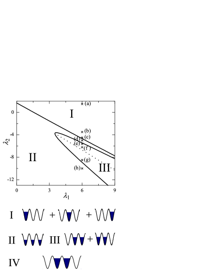
Figure 1: (Color online) The norm distribution and the structure of the localized states with two-body interactions ($\lambda_{1}$) and three-body interactions ($\lambda_{2}$). The solid lines are the boundaries dividing phases I-III. The dotted line presents the critical value $\lambda_{2}^{*}$ with $\lambda_{1}$. When $\lambda_{2}=\lambda_{2}^{*}$ the DK is the most stable one. The symbols (a)-(h) correspond to the sets of parameters $(\lambda_{1},\lambda_{2})$ used in Fig. 2. Phase IV is gained by Eq. (17) which corresponds to a four-site model.

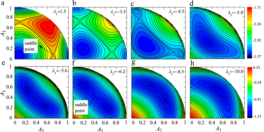
Figure 2: (Color online) Contour plots of the lower PN energy landscape $H_{PN}^{l}$ for different $\lambda_{2}$ with fixed $\lambda_{1}=6$. (a)-(h) correspond to the points a-f marked in Fig. 1. In (a)-(c), the three minima are separated by the two saddle points and DB exists. In (d) and (h), no saddle point exists, which means there is no any kind of localized modes. In (e)-(g), two minima are separated by one saddle point and DK exists. The color codes present the energy of $H_{PN}^{l}$.

The structure of MUB in the extended lattices is similar to that of a DK. MUB is a four-site solution of the DNLS, with high atomic density concentrated mainly at two middle sites and two low-density sites. Up to now, there are few studies on the properties of MUB, especially on its stability. Here we also investigate the effect on transfer of BECs through the MUB from the on-site two- and three-body interactions. It can be investigated by using four-site model, i.e., $M=4$. Eq. (9) becomes

$$\begin{split}i\partial_{t}\psi_{1}&=\lambda_{1}\left|\psi_{1}\right|{}^{2}\psi_{1}+\lambda_{2}\left|\psi_{1}\right|{}^{4}\psi_{1}-\frac{1}{2}\psi_{2},\\ i\partial_{t}\psi_{2}&=\lambda_{1}\left|\psi_{2}\right|{}^{2}\psi_{2}+\lambda_{2}\left|\psi_{2}\right|{}^{4}\psi_{2}-\frac{1}{2}\left(\psi_{1}+\psi_{3}\right),\\ i\partial_{t}\psi_{3}&=\lambda_{1}\left|\psi_{3}\right|{}^{2}\psi_{3}+\lambda_{2}\left|\psi_{3}\right|{}^{4}\psi_{3}-\frac{1}{2}\left(\psi_{2}+\psi_{4}\right),\;\;\\ i\partial_{t}\psi_{4}&=\lambda_{1}\left|\psi_{4}\right|{}^{2}\psi_{4}+\lambda_{2}\left|\psi_{4}\right|{}^{4}\psi_{4}-\frac{1}{2}\psi_{3}.\end{split}$$ (16)

Here, the normalization reads $N=\sum_{n=1}^{4}\left|\psi_{n}\right|{}^{2}=1$. Similarly, by setting $\delta\theta_{12}=\delta\theta_{23}=\delta\theta_{34}=\pi$, one can get

$$\begin{split}\lambda_{1}\!\!\left(A_{1}^{2}\!-\!A_{2}^{2}\right)\!&+\!\lambda_{2}\!\!\left(A_{1}^{4}\!-\!A_{2}^{4}\right)\!+\!\frac{1}{2}\!\left(\frac{A_{2}}{A_{1}}\!-\!\frac{A_{1}+A_{3}}{A_{2}}\right)\!\!=0,\\ \lambda_{1}\!\!\left(A_{2}^{2}\!-\!A_{3}^{2}\right)\!&+\!\lambda_{2}\!\!\left(A_{2}^{4}\!-\!A_{3}^{4}\right)\!+\!\frac{1}{2}\!\left(\frac{A_{1}+A_{3}}{A_{2}}\!-\!\frac{A_{2}+A_{4}}{A_{3}}\right)\!\!=0,\\ \lambda_{1}\!\!\left(A_{3}^{2}\!-\!A_{4}^{2}\right)\!&+\!\lambda_{2}\!\!\left(A_{3}^{4}\!-\!A_{4}^{4}\right)\!+\!\frac{1}{2}\!\left(\frac{A_{2}+A_{4}}{A_{3}}\!-\!\frac{A_{3}}{A_{4}}\right)\!\!=0.\end{split}$$ (17)

By solving Eq. (17), one can get the MUB and the saddle points.

Now, let us discuss the stability and dynamics of DB and DK on phases I and III in which the system has saddle points (i.e., the system has the Peierls-Nabarro barriers), excluding phase II in which there is only one stationary state without saddle points. As shown in previous works BRumpf2004 ; HHennig2013 , if there is no saddle point, the system should be in a random (generic) state in the presence of boundary or other local dissipation, and cannot form any kind of localized modes. That is, for the system with parameters of phase II, the localized mode does not occur. Although phase IV cannot be shown in Fig. 2 as there are not enough dimensions, saddle points can still exist and they are also investigated here.

III Stability of localized states

The contours of the lower PN energy landscape $H_{PN}^{l}$ for different $\lambda_{2}$ with fixed $\lambda_{1}=6$ are shown in Fig. 2(a)-(h). Fig. 2(a)-(c) corresponds to phase I in Fig. 1 and there exist three stationary points and two saddle points. That is, the norm can be localized in three different ways (see Fig. 1) and DB exists. Fig. 2(e)-(g) corresponds to phase III in Fig. 1 and there exist two stationary points and one saddle point [this case cannot exist in the system without three-body interactions, as shown in Fig. 1 with $\lambda_{2}=0$]. This case corresponds to DK. Fig. 2(d) and (h) corresponds to phase II in Fig. 1 and there exists only one stationary point but no saddle point.

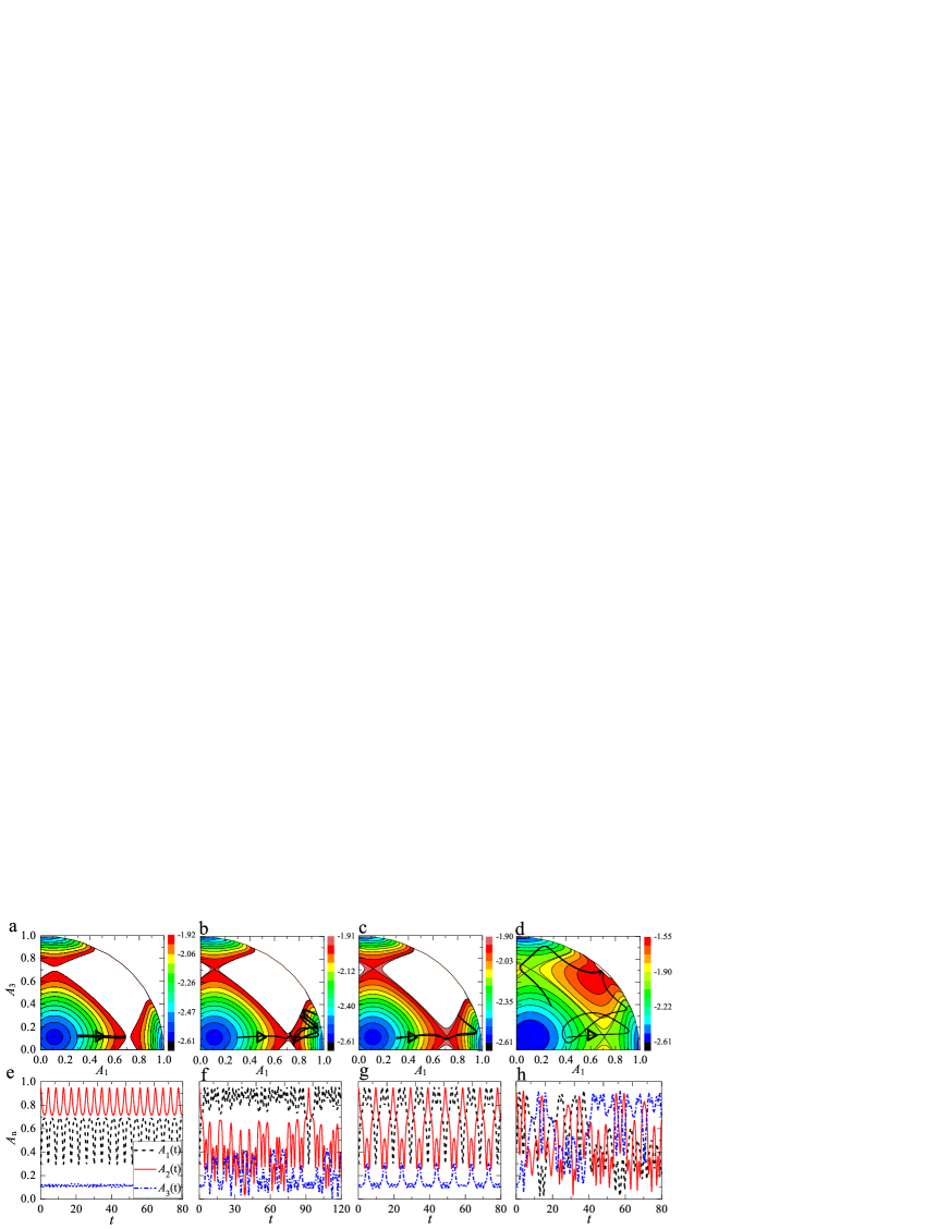
Figure 3: (Color online) Dynamics of the trimer when its total energy is increased with fixed two-body interactions $\lambda_{1}=6$ and three-body interactions $\lambda_{2}=-1.5$, where $E_{thr1}=-1.91469$. A projection of the orbit onto the $A_{1}-A_{3}$ plane is over-plotted (black curve) in (a)-(d). (a) and (e) $E_{t}=-1.9176<E_{thr1}$, areas in phase space are disconnected and the amplitudes $A_{n}(t)$ indicate that the maximum amplitude remains at site 2, i.e., the DB is stable; (b) and (f) $E_{t}=-1.91179>E_{thr1}$, areas in phase space are connected. A slight instability of the DB centered at site 2 is observed, the breather migrates to site 1, and then tangles in site 1; (c) and (g) for a high total energy $E_{t}=-1.8995$, the norm is transmitted to site 1, tangles, and then comes back; (d) and (h) for an enough high total energy $E_{t}=-1.5504$, the orbit explores large parts of the phase space and visits all three sites. In all cases $\delta_{\theta}=\pi$.

III.1 The stability and dynamics of DB

To study the transfer of BEC through the DB in an optical lattice with three-body interactions, we should pay attention to the energy threshold $E_{thr}$ and energy $E_{DB}$ again. In this case, for $\lambda_{1}\rightarrow\infty$ and $\lambda_{2}/\lambda_{1}\rightarrow 0$, one can get the saddle point from Eq. (10) as

$$\begin{split}A_{1}&\approx\frac{1}{\sqrt{2}}+\frac{\lambda_{2}^{2}}{\sqrt{2}\lambda_{1}^{3}}+\frac{\lambda_{2}}{2\sqrt{2}\lambda_{1}^{3}},\\ A_{3}&\approx\frac{3}{2\sqrt{2}\lambda_{1}^{3}}-\frac{1}{\sqrt{2}\lambda_{1}^{2}}+\frac{1}{\sqrt{2}\lambda_{1}}-\frac{\lambda_{2}}{2\sqrt{2}\lambda_{1}^{2}}.\end{split}$$ (18)

By substituting the saddle point into Eq. (8) with $A_{1}^{2}+A_{2}^{2}+A_{3}^{2}=1$, one can get the energy threshold

$$E_{\text{thr1}}\!\! = \!-\!\frac{\lambda_{1}}{4}-\frac{1}{2}-\frac{1}{4\lambda_{1}}+\frac{1}{4\lambda_{1}^{2}}-\!\!\frac{1}{4\lambda_{1}^{3}}+\frac{9}{16\lambda_{1}^{4}}-\frac{3}{2\lambda_{1}^{5}}$$

$$\!-\!\!\left(\frac{1}{12}-\frac{1}{8\lambda_{1}^{2}}+\frac{1}{4\text{ }\lambda_{1}^{3}}-\frac{3}{8\lambda_{1}^{4}}+\frac{5}{8\lambda_{1}^{5}}\right)\!\!\lambda_{2}$$

$$\!-\!\!\left(\frac{1}{16\lambda_{1}^{3}}\!-\!\frac{3}{16\lambda_{1}^{4}}\!-\!\frac{1}{2\lambda_{1}^{5}}\right)\!\!\lambda_{2}^{2}+\!\!\left(\frac{1}{32\lambda_{1}^{4}}\!-\!\frac{5}{4\lambda_{1}^{5}}\right)\!\!\lambda_{2}^{3}.$$

Of course, $E_{DB}$ can also be obtained by substituting the bright breather given by Eq. (10) into Eq. (8).

Next, we consider the fixed point corresponding to the bright breather which is gained from Eq. (10). An initial condition for the bright breather reads $\overrightarrow{\psi}^{DB}(0)=(A_{1}^{DB},A_{2}^{DB},A_{3}^{DB})$. We add perturbations to site 1: $\overrightarrow{\psi}{(t=0)}=((A_{1}^{DB}+\delta_{A_{1}})e^{i\delta_{\theta}},A_{2},A_{3}^{DB})$, where $A_{2}=(1-|\psi_{1}|^{2}-|\psi_{3}|^{2})^{1/2}$. Compared to the bright breather, we add an amplitude $\delta_{A_{1}}$ to site $1$ and rotate the phase $\theta_{1}$ by $\delta_{\theta}$. Dynamics on the PN landscape for increasing total energy of the trimer with fixed two-body interactions $\lambda_{1}=6$ and three-body interactions $\lambda_{2}=-1.5$ is shown in Fig. 3. Here $E_{thr1}=-1.91469$, and we fix $\delta_{\theta}=\pi$ and increase $\delta_{A_{1}}$ in Fig. 3(a)-(d). If the perturbation is small, $E_{t}<E_{thr1}$, the areas in phase space are disconnected. Furthermore, the DB is stable and practically no transfer of norm takes place on short time scales [see Fig. 3(a) and (e)]. If the perturbation is large, $E_{t}>E_{thr1}$, the areas in phase space are connected [see Fig. 3(b) and (c)]. Instability of the DB centered at site 2 can be observed, that is, the breather migrates to site 1 and norm is transferred to site 3 [see Fig. 3(b), (c), (f), and (g)]. If the perturbation is large enough, the orbit goes out of the regular island into the chaotic sea [see Fig. 2(d)] and large amplitudes $A_{n}(t)$ are found at all the three sites, as depicted in Fig. 3(h).

Figure 4: (Color online) (a) Energy difference $\Delta E$ and (b) perturbations $\delta A_{1}$ for destabilizing the DB as a function of three-body interactions $\lambda_{2}$. Different lines indicate three different values of $\lambda_{1}$, respectively. The left and right of the dotted line present attractive (i.e., $\lambda_{2}<0$) and repulsive (i.e., $\lambda_{2}>0$) three-body interactions, respectively. $\delta\theta_{12}=\pi/4$ in (b).

Further, we use the parameters $\delta A_{1}$ and $\Delta E$ to investigate the effect of the two- and three-body interactions on the stability of DB, shown in Fig. 4. It is clear that both $\Delta E$ and $\delta A_{1}$ increase with $\lambda_{1}$ whether three-body interactions are repulsive or attractive (i.e., $\lambda_{2}>$ or $\lambda_{2}<0$), which means that a larger perturbation is required to destabilize the DB when $\lambda_{1}$ increases and on-site two-body interactions can stabilize the DB. Interestingly, both $\Delta E$ and $\delta A_{1}$ increase with repulsive three-body interactions ($\lambda_{2}>0$) but decrease with attractive three-body interactions ($\lambda_{2}<0$), which means that a relatively large perturbation is needed to destabilize the DB when repulsive three-body interactions increase. When attractive three-body interactions increase, a relatively small perturbation is needed to destabilize the DB. That is, repulsive on-site three-body interactions can stabilize the DB, while attractive on-site three-body interactions destabilize the DB. For large enough attractive on-site three-body interactions, $\Delta E=\delta A_{1}=0$ and the DB is completely unstable.

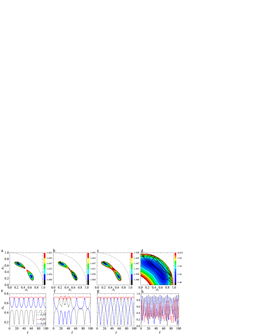
Figure 5: (Color online) Dynamics of the trimer when its total energy is increased with fixed two-body interactions $\lambda_{1}=6$ and three-body interactions $\lambda_{2}=-7.5$, where $E_{thr2}=-1.44281$. A projection of the orbit onto the $A_{1}-A_{3}$ plane is over-plotted (black curve) in (a)-(d). (a) A contour plot of the lower PN energy landscape $H_{PN}^{l}$ is shown for the total energy of the trimer below the threshold ($E_{t}=-1.44304<E_{thr2}$). Obviously, the areas in phase space are disconnected. (e) The amplitudes $A_{n}(t)$ with time $t$ indicate that the dominating amplitude remains at sites 2 and 3, i.e., the norm is still localized in sites 2 and 3 and the DK is stable. (b) and (f) for total energy $E_{t}=-1.44238>E_{thr2}$, areas in phase space are connected. A slight instability of the DK centered at site 1 is observed. The DK migrates to site 1 and then tangled at site 1 or 3, but the norm of site 2 is nearly constant. (c) and (g) for a high total energy $E_{t}=-1.43809>E_{thr2}$, the DK migrates to site 1 and then come back more easily. Long-range and long-lived Josephson oscillations between sites 1 and 3 with negligible variation of norm in site 2 are observed. i.e., the DK is unstable and the dominating amplitude does not remain at sites 2 and 3. (d) and (h) for an enough high total energy $E_{t}=-0.871835$, the orbit is out of the regular island into the chaotic sea, and the dominating amplitude can be found in any of the three sites, which means the DK is unstable. In all cases $\delta_{\theta}=0$.

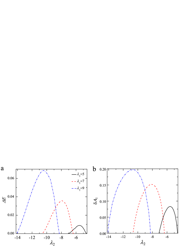
Figure 6: (a) (Color online) Energy difference $\Delta E$ and (b) perturbations $\delta A_{1}$ for destabilizing the DK as a function of three-body interactions $\lambda_{2}$. Different lines indicate three different values of $\lambda_{1}$, respectively. $\lambda_{2}^{*}$ is a critical value of $\lambda_{2}$. When $\lambda_{2}=\lambda_{2}^{*}$, the DK is the most stable one for the fixed $\lambda_{1}$. $\delta\theta_{12}=0$ in (b).

III.2 The stability and dynamics of DK

One can investigate the stability and dynamics of DK with the same way used above. When $\lambda_{2}\rightarrow-\infty$ and $\lambda_{1}/\lambda_{2}\rightarrow 0$, one can get the saddle point from Eq. (10) as

$$\!\!\!\!A_{1}\!=\!A_{3}\approx\!\frac{1}{\sqrt{3}}+\!\frac{\sqrt{3}}{8\lambda_{2}}+\!\frac{54\sqrt{3}}{128\lambda_{2}^{2}}-\!\frac{3\sqrt{3}\lambda_{1}}{8\lambda_{2}^{2}}+\!\frac{513\sqrt{3}}{256\lambda_{2}^{3}}.$$ (20)

By substituting the saddle point into Eq. (8) with $A_{1}^{2}+A_{2}^{2}+A_{3}^{2}=1$, one can get the energy threshold

$$\!\!E_{\text{thr2}}\!\!\!\! = \!\!\!\!\left(\!\!-\frac{\lambda_{2}}{27}\!-\!\frac{2}{3}+\frac{1}{8\lambda_{2}}\!+\!\frac{29}{64\lambda_{2}^{2}}\!+\!\frac{981}{512\lambda_{2}^{3}}\!+\!\frac{151119}{16384\lambda_{2}^{4}}\right)$$ (21)

$$\!\!\!-\!\!\left(\frac{1}{6}+\frac{3}{16\lambda_{2}^{2}}\!+\!\frac{45}{32\lambda_{2}^{3}}\!+\!\frac{9369}{1024\lambda_{2}^{4}}\!+\!\frac{3013119}{32768\lambda_{2}^{5}}\right)\!\!\lambda_{1}$$

$$\!\!+\!\!\left(\frac{135}{16\lambda_{2}^{4}}+\frac{243}{8\lambda_{2}^{5}}\right)\!\!\lambda_{1}^{2}\!\!-\!\!\left(\frac{27}{16\lambda_{2}^{4}}+\!\frac{189}{128\lambda_{2}^{5}}\right)\!\!\lambda_{1}^{3}.$$

Next, we consider the fixed point corresponding to the DK which is also gained from Eq. (10). The initial condition for the DK reads $\overrightarrow{\psi}^{DK}(t=0)=(A_{1}^{DK},A_{2}^{DK},A_{3}^{DK})$. One can add perturbations to site 1: $\overrightarrow{\psi}{(0)}=((A_{1}^{DK}+\delta_{A_{1}})e^{i\delta_{\theta}},A_{2},A_{3}^{DK})$, where $A_{2}=(1-|\psi_{1}|^{2}-|\psi_{3}|^{2})^{1/2}$. Dynamics on the PN landscape for increasing total energy of the trimer with fixed two-body interactions $\lambda_{1}=6$ and three-body interactions $\lambda_{2}=-7.5$ is shown in Fig. 5. Here $E_{thr2}=-1.44281$. If the perturbation is small, $E_{t}<E_{thr}$, the areas in phase space are disconnected. The DK is stable and the norm is localized nearly in the adjacent two sites $2$ and $3$ on short time scales, shown in Fig. 5(a) and (e). If $E_{t}$ is just larger than $E_{thr}$, the areas in phase space are connected and instability of the DK can be observed; that is, the DK migrates from site $3$ to site $1$ and then tangles at $1$ or $3$, but the norm of site $2$ [presented by $A_{2}(t)$] is nearly constant, shown in Fig. 5(b) and (f). If the perturbation becomes larger, one can see that there are long-range and long-lived Josephson oscillations between sites 1 and 3 with negligible variation of norm in site 2, shown in Fig. 5(c) and (g). If the perturbation is large enough, the orbit explores large parts of space and visits all three sites, shown in Fig. 5(d), and large amplitudes $A_{n}(t)$ can be found at all three sites, shown in Fig. 5(h).

One can also use $\delta A_{1}$ and $\Delta E$ to investigate the stability of DK, shown in Fig. 6. For a fixed $\lambda_{1}$, one can see that both $\Delta E$ and $\delta A_{1}$ first increase and then decrease with $\lambda_{2}$. That is, there exists a critical three-body interaction $\lambda_{2}^{*}$ with which the DK is the most stable one. When $\lambda_{2}\neq\lambda_{2}^{*}$, the DK becomes more unstable when $\lambda_{2}$ decreases or increases. Furthermore, we numerically get the critical value when $\lambda_{1}>3.5$

$$\lambda_{2}^{*} = 0.27034-1.13186\lambda_{1}+0.00516\lambda_{1}^{2}.$$ (22)

It is presented by the dotted line in phase III in Fig. 1.

Obviously, the stability of the DK depends strongly on both two- and three-body interactions, while the DK is more unstable than the ordinary DB.

III.3 The stability and dynamics of MUB

For MUB, the lower PN energy landscape in Eq. (4) becomes

$$\!\!H_{\text{PN}}^{l}\!\! \!\!=\!\! \!-\!\frac{\lambda_{1}}{2}\!\left(\!A_{1}^{4}\!+\!A_{2}^{4}\!+\!A_{3}^{4}\!+\!A_{4}^{4}\right)\!\!-\!\!\frac{\lambda_{2}}{3}\!\left(\!A_{1}^{6}\!+\!A_{2}^{6}\!+\!A_{3}^{6}\!+\!A_{4}^{6}\right)\;\;\;\;$$ (23)

$$\!-\left(A_{1}A_{2}+A_{2}A_{3}+A_{3}A_{4}\right).$$

When $\lambda_{2}\rightarrow-\infty$ and $\lambda_{1}/\lambda_{2}\rightarrow 0$, one can get the saddle point from Eq. (17) as

$$A_{1} \!\!\approx\!\! \frac{1}{\sqrt{3}}+\frac{\sqrt{3}}{8\lambda_{2}}+\frac{54\sqrt{3}}{128\lambda_{2}^{2}}-\frac{3\sqrt{3}\lambda_{1}}{8\lambda_{2}^{2}}+\frac{513\sqrt{3}}{256\lambda_{2}^{3}},$$

$$A_{3} \!\!\approx\!\! \frac{1}{\sqrt{3}}+\frac{\sqrt{3}}{8\lambda_{2}}-\frac{54\sqrt{3}}{128\lambda_{2}^{2}}-\frac{3\sqrt{3}\lambda_{1}}{8\lambda_{2}^{2}}+\frac{513\sqrt{3}}{256\lambda_{2}^{3}},$$

$$A_{4} \!\!\approx\!\! \frac{27\sqrt{3}}{4\lambda_{2}^{2}}.$$ (24)

By substituting the saddle point into Eq. (23) with $A_{1}^{2}+A_{2}^{2}+A_{3}^{2}+A_{4}^{2}=1$, one can get the energy threshold

$$\!\!\!\!\!\!\!E_{\text{thr3}}\!\!\!\! = \!\!\!\!-\frac{\lambda_{2}}{27}-\frac{2}{3}+\frac{1}{8\lambda_{2}}-\frac{\lambda_{1}}{6}-\frac{403+12\lambda_{1}}{64\lambda_{2}^{2}}$$ (25)

$$\!\!\!\!-\frac{3\left(-8541+3072\lambda_{1}+640\lambda_{1}^{2}\right)}{2048\lambda_{2}^{3}}$$

$$\!\!\!\!+\frac{9\left(103827\!+\!61338\lambda_{1}\!+\!8032\lambda_{1}^{2}\!-\!3584\lambda_{1}^{3}\right)}{8192\lambda_{2}^{4}}.$$

Suppose that the initial condition for the MUB is $\overrightarrow{\psi}^{MUB}(t=0)=(A_{1}^{MUB},A_{2}^{MUB},A_{3}^{MUB},A_{4}^{MUB})$. One can add perturbations to site 1: $\overrightarrow{\psi}{(0)}=((A_{1}^{MUB}+\delta_{A_{1}})e^{i\delta_{\theta}},A_{2},A_{3}^{MUB},A_{4}^{MUB})$, where $A_{2}=(1-|\psi_{1}|^{2}-|\psi_{3}|^{2}-|\psi_{4}|^{2})^{1/2}$. Dynamics of the MUB for increasing total energy of the four-site system with $\lambda_{1}=6$ and $\lambda_{2}=-7$ is shown in Fig. 7. Here $E_{thr3}=-1.50027$. If there is no perturbation, i.e., $\delta A_{1}=\delta\theta=0$, the MUB is stable absolutely and the norm is localized in the middle adjacent two sites $2$ and $3$ with $A_{2}(t)=A_{3}(t)$ and $A_{1}(t)=A_{4}(t)$, shown in Fig. 7(a). If the perturbation is small, $E_{t}<E_{thr3}$, the MUB is stable and the norm is localized nearly in the adjacent two middle sites $2$ and $3$, shown in Fig. 7(b). In contrast, if $E_{t}$ is just larger than $E_{thr3}$, the MUB becomes unstable after $t\approx 78$ time steps, and the MUB migrates from sites $2$ and $3$ to sites $3$ and $4$ or $1$ and $2$, shown Fig. 7(c). Similarly, if the perturbation is large enough, the stability of the MUB is destroyed, shown in Fig. 7(d).

Also, one can use $\delta A_{1}$ and $\Delta E$ to investigate the stability of MUB, shown in Fig. 8. For a fixed $\lambda_{1}$, both $\Delta E$ and $\delta A_{1}$ first increase with $\lambda_{2}$ before decreasing. That is, there still exists a critical three-body interaction $\lambda_{2}^{*}$ at which the MUB is the most stable one. When $\lambda_{2}\neq\lambda_{2}^{*}$, the MUB becomes unstable when $\lambda_{2}$ decreases or increases.

Figure 7: (Color online) Dynamics of MUB for increasing the total energy of the four-site system with $\lambda_{1}=6$ and $\lambda_{2}=-7$, where $E_{thr3}=-1.50027$. (a) $\delta_{A}=\delta_{\theta}=0$, the MUB is absolutely stable, and $A_{1}(t)=A_{4}(t)$ and $A_{2}(t)=A_{3}(t)$. (b) $\delta_{\theta}=\pi/3.4$, $E_{t}=-1.50212<E_{thr3}$, the multi-breather is stable, and it is still located at sites $2$ and $3$. (c) $\delta_{\theta}=\pi/2.8$, $E_{t}=-1.47925$ is just larger than $E_{thr3}$, the multi-breather is unstable, and the norm from sites $2$ and $3$ migrate to sites $3$ and $4$ after $t\approx 78$ time steps. (d) $\delta_{\theta}=\pi/2$, $E_{t}=-1.42046>E_{thr3}$, the stability of the multi-breather is destroyed, and the dominating amplitude can be found in any of the four sites. In all cases $\delta_{A_{1}}=0$. Initial conditions are given by Eq. (17).

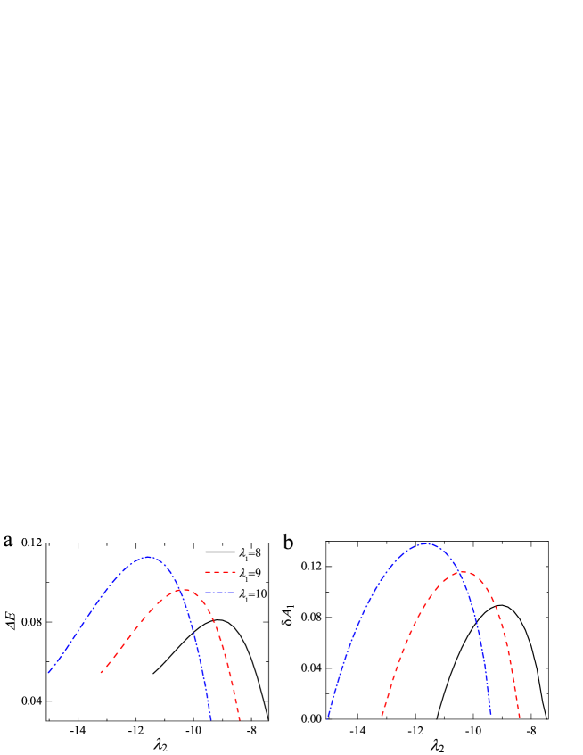
Figure 8: (Color online) (a) Energy difference $\Delta E$ and (b) perturbations $\delta A_{1}$ for destabilizing the MUB as a function of three-body interactions $\lambda_{2}$. Different lines indicate three different values of $\lambda_{1}$, respectively. The $\lambda_{2}^{*}$ is a critical value of $\lambda_{2}$. When $\lambda_{2}=\lambda_{2}^{*}$, the MUB is the most stable for the fixed $\lambda_{1}$. $\delta\theta_{12}=\pi/3.4$ in (b).

IV Extended lattices

Now, let us generalize our study to the case with extended lattices, i.e., $M>4$.

IV.1 DB in extended lattices

Here we use the same initial conditions as the case with three sites, i.e., $\lambda_{1}=6$, $\lambda_{2}=-1.5$, to study an extended lattice system. We assume $M=101$ and the DB locates at the site $n=51$. The initial condition reads

$$\begin{split}\psi_{50}(0)&=(A_{1}^{DB}+\delta_{A_{1}})e^{i\delta_{\theta}},\\ \psi_{51}(0)&=A_{2},\\ \psi_{52}(0)&=A_{1}^{DB},\\ \psi_{n}(0)&=0,\;\;\texttt{else},\end{split}$$ (26)

where $A_{2}=(1-|\psi_{50}|^{2}-|\psi_{52}|^{2})^{1/2}$ and $A_{1}^{DB}$ is obtained exactly from Eq. (10). The wave function is normalized to $\sum_{n=1}^{M}|\psi_{n}|^{2}=1$. The stability and migration of a DB in extended lattices ($M=101$ sites) is shown in Fig. 9. The solution for the DB in the trimer, i.e., the initial condition shown in Eq.(26), is inserted in the extended lattice. Here $E_{thr1}=-1.91469$ when $\lambda_{1}=6$ and $\lambda_{2}=-1.5$ (corresponding to Fig. 3). Obviously, when no perturbation is added to the site $50$, i.e., $\delta_{A_{1}}=\delta_{\theta}=0$, the breather is stable, shown in Fig. 9(a) and (d). When the perturbation is added to the site $50$ and the total energy of the local trimer $E_{t}$ is just larger than $E_{thr1}$, the breather is stable and no migration takes place, different from the case with three sites, shown in Fig. 9(b) and (e). The reason is that the energy can flow into additional degrees of freedom in extended lattices. When the perturbation is large and the total energy of the local trimer $E_{t}>E_{thr1}$, the breather is destabilized and migrates from site $51$ to site $50$ after $t\approx 2$ time steps, similar to the case with the three-site model, shown in Fig. 9(c) and (f).

Figure 9: (Color online) The stability and migration of a DB in extended lattices ($M=101$ sites). The color code represents $|\psi_{n}(t)|$. The insert in (a) represents the structure of DB. Initial conditions are given by Eq. (26) with (a) $\delta_{A}=\delta_{\theta}=0$, $E_{t}=-2.61029<E_{thr1}$, (b) $\delta_{A}=0.184$, $\delta_{\theta}=\pi$, $E_{t}=-1.91179$ is just larger than $E_{thr1}$, (c) $\delta_{A}=0.199$, $\delta_{\theta}=\pi$, $E_{t}=-1.87136>E_{thr1}$. In all cases $\lambda_{1}=6$ and $\lambda_{2}=-1.5$.

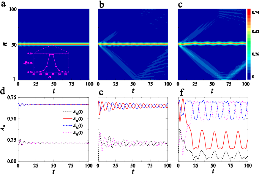
Figure 10: (Color online) The stability and migration of a MUB in extended lattices ($M=101$ sites). The color code represents $|\psi_{n}(t)|$. The insert in (a) represents the structure of MUB. Initial conditions are given by Eq. (17) with (a) $\delta_{A}=\delta_{\theta}=0$, $E_{t}=-1.55596<E_{thr3}$, (b) $\delta_{\theta}=\pi/2.8$, $E_{t}=-1.47925$ is just larger than $E_{thr1}$, (c) $\delta_{\theta}=\pi/1.79$, $E_{t}=-1.39563>E_{thr3}$. In all cases $\lambda_{1}=6$ and $\lambda_{2}=-7$.

IV.2 MUB in extended lattices

For MUB, we use the same initial condition as the case with the four-site model to study its stability and dynamics in the extended lattice system (M=101 sites), i.e., $\lambda_{1}=6$ and $\lambda_{2}=-7$. Here, the MUB is located at the sites $n=51$ and $n=52$. The initial condition reads

$$\begin{split}\psi_{50}(0)&=(A_{1}^{MUB}+\delta_{A_{1}})e^{i\delta_{\theta}},\\ \psi_{51}(0)&=A_{2},\\ \psi_{52}(0)&=A_{2}^{MUB},\\ \psi_{53}(0)&=A_{1}^{MUB},\\ \psi_{n}(0)&=0,\;\;\texttt{else},\end{split}$$ (27)

where $A_{2}=(1-|\psi_{50}|^{2}-|\psi_{52}|^{2}-|\psi_{53}|^{2})^{1/2}$ and $A_{1}^{MUB}$ and $A_{2}^{MUB}$ are obtained exactly from Eq. (17). The wave function is normalized to $\sum_{n=1}^{M}|\psi_{n}|^{2}=1$. The solution for the MUB in the four-site model is inserted in the extended lattice. Here $E_{thr3}=-1.50027$ when $\lambda_{1}=6$ and $\lambda_{2}=-7$. Obviously, when no perturbation is added to site $50$, i.e., $\delta_{A_{1}}=\delta_{\theta}=0$, the breather is stable, shown in Fig. 10(a) and (d). As $|\psi_{50}(t)|=|\psi_{53}(t)|$ and $|\psi_{51}(t)|=|\psi_{52}(t)|$, the red and the blue lines are overlapped, and the black and the green lines are overlapped in Fig. 10(d). When the perturbation is added to site $50$ and the total energy $E_{t}$ is just larger than $E_{thr3}$, the energy can flow into additional degrees of freedom in extended lattices, and the MUB is still stable and no migration takes place, shown in Fig. 10(b) and (e). When the perturbation is larger and the total energy $E_{t}>E_{thr3}$, the MUB is destabilized and migrates from site $51$ to site $53$ and locate in sites $52$ and $53$ after $t\approx 14$ time steps, shown in Fig. 10(c) and (f).

From the discussion above, one can see that the stability and the dynamics characters of both DB and MUB are general for extended lattices.

V Discussion and summary

Although the three-body interactions could be observed or realized in experiment and theory SWill2010 ; DaleyAJ2014 , there are no systematical analysis of their type, existence, and stability of the localized modes. Previous works indicated that DB can exist and its stability plays a crucial role in blocking, filtering, and transfer in BECs GPTsironis1996 ; RLivi2006 ; GSNg2009 ; BRumpf2004 . The exact condition to destabilize DB is still not clear, especially in the case by considering three-body interactions. Recent works GSNg2009 ; RFranzosi2011 showed that MUB can exist for BECs in optical lattices by only considering two-body interactions in the case with large interactions and appropriate phases.

In our work, we systematically investigated the existence of the different localized modes for different parameters $(\lambda_{1},\lambda_{2})$, i.e., DB, DK, and MUB, and discussed the effect of two- and three-body interactions on their stabilities. Both on-site repulsive two- and three-body interactions can stabilize DB, while on-site attractive three-body interactions destabilize DB. DK and MUB are the most stable ones when the three-body interactions are equal to a critical value for the fixed two-body interactions. It may provide effective guidance to gain different kinds of localized modes in optical lattices HHennig2013 ; RLivi2006 and help us to study its properties in experiment, especially for MUB.

Besides, in our work, three analyzed thresholds to destabilize the three localized modes are given explicitly. If the total energy of the system is higher than the energy thresholds, the localized state is unstable. On the contrary, if the total energy of the system is lower than the energy thresholds, the localized state is stable. It may lead to some interesting applications for blocking and filtering atom beams when there are both two- and three-body interactions in the system. Furthermore, it is useful for controlling the transmission of matter waves in interferometry and quantum-information processes RAVicencio2007 .

In summary, we have investigated the stability and phase transition of localized modes in BECs in an optical lattice with the discrete nonlinear Schrödinger model by considering two- and three-body interactions. It has been shown that there are three different types of localized modes. The first one is bright DB which can be stabilized by both on-site repulsive two- and three-body interactions. However, on-site attractive three-body interactions destabilize DB. The second one is DK which is the most stable one when the three-body interaction is equal to a critical value for fixed two-body interactions. The third one is MUB. It becomes the most stable one when three-body interaction is in the critical value. Moreover, the stability and dynamics characters of DB and MUB are general for extended lattice systems. Our results provide a deep insight into the dynamics of blocking, filtering, and transfer of the norm in nonlinear lattices for BECs by considering both two- and three-body interactions.

References

- (1) Y. Ishimori, T. Munakata, J. Phys. Soc. Jpn. 51 (1982) 3367.
- (2) M. Peyrard, M. D. Kruskal, Physica D 14 (1984) 88.
- (3) A. J. Sievers, S. Takeno, Phys. Rev. Lett. 61 (1988) 970.
- (4) D. K. Campbell, Nature (London) 432 (2004) 455.
- (5) D. K. Campbell, S. Flach, Y. S. Kivshar, Phys. Today 57 (2004) 43.
- (6) S. Flach, A. V. Gorbach, Phys. Rep. 467 (2008) 1.
- (7) H. Hennig, R. Fleischmann, Phys. Rev. A 87 (2013) 033605.
- (8) M. Sato, B. E. Hubbard, A. J. Sievers, Rev. Mod. Phys. 78 (2006) 137.
- (9) U. T. Schwarz, L. Q. English, A. J. Sievers, Phys. Rev. Lett. 83 (1999) 223.
- (10) M. Sato, A. J. Sievers, Nature (London) 432 (2004) 486.
- (11) E. Trias, J. J. Mazo, T. P. Orlando, Phys. Rev. Lett. 84, 741 (2000).
- (12) A. V. Ustinov, Chaos 13 (2003) 716.
- (13) H. S. Eisenberg, Y. Silberberg, R. Morandotti, A. R. Boyd, J. S. Aitchison, Phys. Rev. Lett. 81 (1998) 3383.
- (14) R. Morandotti, U. Peschel, J. S. Aitchison, H. S. Eisenberg, Y. Silberberg, Phys. Rev. Lett. 83 (1999) 2726.
- (15) A. Trombettoni, A. Smerzi, Phys. Rev. Lett. 86 (2001) 2353.
- (16) B. Eiermann, T. Anker, M. Albiez, M. Taglieber, P. Treutlein, K. P. Marzlin, M. K. Oberthaler, Phys. Rev. Lett. 92 (2004) 230401.
- (17) E. B. Kolomeisky, J. P. Straley, Phys. Rev. B 46 (1992) 11749; E. B. Kolomeisky, T. J. Newman, J. P. Straley, X. Qi, Phys. Rev. Lett. 85 (2000) 1146.
- (18) J. K. Xue, A. X. Zhang, Phys. Rev. Lett. 101 (2008) 180401; A. X. Zhang and J. K. Xue Phys. Rev. A 80 (2009) 043617.
- (19) M. G. Clerc, R. G. Elias, R. G. Rojas, Philos. Trans. R. Soc. London Ser. B 369 (2011) 412.
- (20) P. C. Matthews, H. Susanto, Phys. Rev. E 84 (2011) 066207.
- (21) S. Aubry, Physica D 103 (1997) 201.
- (22) J. Dorignac, J. C. Eilbeck, M. Salerno, A. C. Scott, Phys. Rev. Lett. 93 (2004) 025504.
- (23) M. Matuszewski, E. Infeld, B. A. Malomed, M. Trippenbach, Phys. Rev. Lett. 95 (2005) 050403.
- (24) H. Sakaguchi, B. A. Malomed, Phys. Rev. A 81 (2010) 013624.
- (25) N. Boechler, G. Theocharis, S. Job, P. G. Kevrekidis, Mason A. Porter, C. Daraio, Phys. Rev. Lett. 104 (2010) 244302.
- (26) S. Flach, C. R. Willis, Phys. Rep. 295 (1998) 181.
- (27) R. S. MacKay, J. A. Sepulchre, Physica D 119 (1998) 148.
- (28) P. J. Martinez, M. Meister, L. M. Floria, F. Falo, Chaos 13 (2003) 610.
- (29) G. P. Tsironis, S. Aubry, Phys. Rev. Lett. 77 (1996) 5225.
- (30) R. Livi, R. Franzosi, G. L. Oppo, Phys. Rev. Lett. 97 (2006) 060401.
- (31) G. S. Ng, H. Hennig, R. Fleischmann, T. Kottos, T. Geisel, New J. Phys. 11 (2009) 073045.
- (32) Y. Wu, L. Deng, Phys. Rev. Lett. 93 (2004) 143904.
- (33) L. Li, Z. D. Li, Boris A. Malomed, D. Mihalache, W. M. Liu, Phys. Rev. A 72 (2005) 033611.
- (34) Z. X. Liang, Z. D. Zhang, W. M. Liu, Phys. Rev. Lett. 94 (2005) 050402.
- (35) H. Hennig, J. Dorignac, D. K. Campbell, Phys. Rev. A 82 (2010) 053604.
- (36) R. Franzosi, R. Livi, G. L. Oppo, A. Politi, Nonlinearity 24 (2011) R89.
- (37) X. D. Bai, J. K. Xue, Phys. Rev. E 86 (2012) 066605.
- (38) S. Will, T. Best, U. Schneider, L. Hackermüller, D. S. Lühmann, I. Bloch, Nature (London) 465 (2010) 197.
- (39) A. J. Daley, J. Simon, Physical Review A 89 (2014) 053619.
- (40) D. S. Petrov, Phys. Rev. Lett. 112 (2014) 103201 .
- (41) T. Luu, A. Schwenk, Phys. Rev. Lett. 98, (2007) 103202.
- (42) B. L. Chen, X. B. Huang, S. P. Kou, Y. B. Zhang, Phys. Rev. A 78 (2008) 043603.
- (43) P. R. Johnson, E. Tiesinga, J. V. Porto, C. J. Williams, New J. Phys. 11 (2009) 093022.
- (44) K. Z. Zhou, Z. X. Liang, Z. D. Zhang, Phys. Rev. A 82 (2010) 013634.
- (45) S. Inouye, M. R. Andrews, J. Stenger, H. J. Miesner, D. M. Stamper-Kurn, W. Ketterle, Nature (London) 392 (1998) 151.
- (46) R. Dasgupta, Phys. Rev. A 82 (2010) 063607.
- (47) M. Singh, A. Dhar, T. Mishra, R. V. Pai, B. P. Das, Phys. Rev. A 85, (2012) 051604.
- (48) J. M. Speight, Nonlinearity 12 (1999) 1373 .
- (49) P. G. Kevrekidis, B. A. Malomed, A. R. Bishop, Phys. Rev. E 66 (2002) 046621.
- (50) Y. A. Kosevich, R. Khomeriki, S. Ruffo, Europhys. Lett. 66 (2004) 21.
- (51) Y. S. Kivshar, D. K. Campbell, Phys. Rev. E 48, (1993) 3077.
- (52) B. Rumpf, Phys. Rev. E 70, (2004) 016609.
- (53) A. X. Zhang, J. K. Xue, Phys. Lett. A 372 (2008) 1147.
- (54) B. B. Baizakov, A. Bouketir, A. Messikh, B. A. Umarov, Phys. Rev. E 79 (2009) 046605.
- (55) E. Wamba, A. Mohamadou, T. B. Ekogo, J. Atangana, T. C. Kofane, Phys. Lett. A, 375, (2011) 4288.
- (56) R. A. Vicencio, J. Brand, S. Flach, Phys. Rev. Lett. 98 (2007) 184102.