On the critical parameters of the $q\geq 4$ random-cluster model on isoradial graphs

Abstract

The critical surface for random-cluster model with cluster-weight $q\geq 4$ on isoradial graphs is identified using parafermionic observables. Correlations are also shown to decay exponentially fast in the subcritical regime. While this result is restricted to random-cluster models with $q\geq 4$, it extends the recent theorem of [6] to a large class of planar graphs. In particular, the anisotropic random-cluster model on the square lattice is shown to be critical if $\frac{p_{v}p_{h}}{(1-p_{v})(1-p_{h})}=q$, where $p_{v}$ and $p_{h}$ denote the horizontal and vertical edge-weights respectively. We also mention consequences for Potts models.

1 Introduction

1.1 Motivation

Random-cluster models are dependent percolation models introduced by Fortuin and Kasteleyn in 1969 [25]. They have been an important tool in the study of phase transitions. Among other applications, the spin correlations of Potts models get rephrased as cluster connectivity properties of their random-cluster representations, which allows for the use of geometric techniques, thus leading to several important applications. Nevertheless, only few aspects of the random-cluster models are known in full generality.

The random-cluster model on a finite connected graph $G=(\mathcal{V}[G],\mathcal{E}[G])$ is a model on edges of this graph, each one being either closed or open. A configuration can be seen as a random graph, whose vertex set is $\mathcal{V}[G]$ and whose edge set is the collection of all open edges; a cluster is a connected component for this random graph. The probability of a configuration is proportional to

$$\prod_{e\text{~{}open}}p_{e}\prod_{e\text{~{}closed}}(1-p_{e})\cdot q^{\#\;\text{clusters}},$$

where the edge-weights $p_{e}\in[0,1]$ (for every $e\in\mathcal{E}[G]$) and the cluster-weight $q\in(0,\infty)$ are the parameters of the model. Extensive literature exists concerning these models; we refer the interested reader to the monograph of Grimmett [27] and references therein.

For $q\geq 1$, the model can be extended to infinite-volume lattices where it exhibits a phase transition. In general, there are no conjectures for the value of the critical surface, i.e. the set of $(p_{e})_{e\in\mathcal{E}[G]}$ for which the model is critical. In the case of planar graphs, there is a connection (related to the Kramers-Wannier duality [37, 38] for the Ising model) between random-cluster models on a graph and on its dual with the same cluster-weight $q$ and appropriately related edge-weights. This relation leads, in the particular case of $\mathbb{Z}^{2}$ (which is isomorphic to its dual) with $p_{e}=p$ for every $e$, to the following natural prediction: the critical point $p_{c}(q)$ is the same as the so-called self-dual point, which has a known value $\sqrt{q}/(1+\sqrt{q})$. This was proved recently in [6] for any $q\geq 1$ (see also [20]). Furthermore, the size of the cluster at the origin was proved to have exponential decay tail if $p<p_{c}(q)$.

The critical point was previously known in three famous cases. For $q=1$, the model is simply Bernoulli bond-percolation, proved by Kesten [35] to be critical at $p_{c}(1)=1/2$. For $q=2$, the self-dual value corresponds to the critical temperature of the Ising model, as first derived by Onsager [43]; one can actually couple realizations of the Ising and random-cluster models to relate the critical points of each, see [27] and references therein for details. Finally, for $q\geq 25.72$, a proof is known based on the fact that the random-cluster model exhibits a first order phase transition; see [39, 40].

A general challenge in statistical physics is to understand the universal behavior, i.e.  the behavior of a certain model, for instance the planar random-cluster model, on different graphs. A large class of graphs, which appeared to be central in different domains of planar statistical physics, is the class of isoradial graphs. An isoradial graph is a planar graph admitting an embedding in the plane in such a way that every face is inscribed in a circle of radius one. In such a case, we will say that the embedding itself is isoradial.

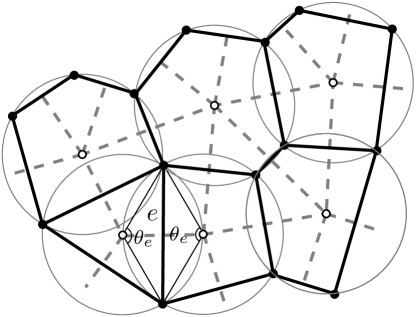
Figure 1: The black graph is the isoradial graph. White vertices are the vertices of the dual graph. All faces can be put into a circumcircle of radius one. Dual vertices have been drawn in such a way that they are the centers of these circles.

Isoradial graphs were introduced by Duffin in [17] in the context of discrete complex analysis. The author noticed that isoradial embeddings form a large class of embeddings for which a discrete notion of Cauchy-Riemann equations is available. Isoradial graphs first appeared in the physics literature in the work of Baxter [1], where they are called $Z$-invariant graphs; the so-called star-triangle transformation was then used to relate the free energy of the eight-vertex and Ising models between different such graphs. In Baxter’s work, $Z$-invariant graphs are obtained as intersections of lines in the plane, and are not embedded in the isoradial way. The term isoradial was only coined later by Kenyon, who studied discrete complex analysis and the graph structure of these graphs [34]. Since then, isoradial graphs were used extensively, and we refer to [9, 14, 30, 34, 42] for literature on the subject.

In the present article, we study the random-cluster model on isoradial graphs.

1.2 Statement of the results

All the graphs which we will consider in this paper will be assumed to be periodic, in the sense that they will carry an action of the square lattice $\mathbb{Z}^{2}$ with finitely many orbits; indeed, this is often a crucial hypothesis in the usual arguments of statistical mechanics. Nevertheless, some of our results extend to a more general family of isoradial graphs, which is why we first introduce the following, weaker condition.

Let $e$ be an edge of an isoradial embedding: it subtends an angle $\theta_{e}\in(0,\pi)$ at the center of the circle corresponding to any of the two faces bordered by $e$; see Fig. 1. Fix $\theta>0$, and let $G_{\infty}=(\mathcal{V}[G_{\infty}],\mathcal{E}[G_{\infty}])$ be an infinite isoradial graph. The graph is said to satisfy the bounded-angle property if the following condition holds:

(BAP_θ)  For any $e\in\mathcal{E}[G_{\infty}]$, $\theta\leq\theta_{e}\leq\pi-\theta$.

In order to study the phase transition, we parametrize random-cluster measures with cluster-weight $q\geq 4$ with the help of an additional parameter $\beta>0$. For $\beta>0$, define the edge-weight $p_{e}(\beta)\in[0,1]$ for $e\in\mathcal{E}[G_{\infty}]$ by the formula

$$\frac{p_{e}(\beta)}{[1-p_{e}(\beta)]\sqrt{q}}=\beta\,\frac{\sinh[\frac{\sigma(\pi-\theta_{e})}{2}]}{\sinh[\frac{\sigma\theta_{e}}{2}]},$$

where the spin $\sigma$ is given by the relation

$$\cosh\big{(}\frac{\sigma\pi}{2}\big{)}=\frac{\sqrt{q}}{2}.$$

The infinite-volume measure on $G_{\infty}$ with cluster-weight $q\geq 4$, edge-weights $(p_{e}(\beta):e\in\mathcal{E}[G_{\infty}])$ and free boundary conditions (see next section for a formal definition) is denoted by $\phi^{0}_{G_{\infty},\beta,q}$.

Remark 1

In the case of the square lattice, one gets $p_{e}(\beta)=\frac{\beta\sqrt{q}}{1+\beta\sqrt{q}}$. This does not quite match what one obtains in the setup of the coupling between the Potts and random-cluster models: the bond-parameter corresponding to the $q$-state Potts model at inverse temperature $\beta$ is equal to $1-e^{-2\beta}$. This simply means that what we will denote here by $\beta$ should not be interpreted as an inverse temperature as such, but simply as a parameter according to which a phase transition can be defined.

Let $|\cdot|$ be the Euclidean norm.

Theorem 2

Let $q\geq 4$, $\theta>0$ and $\beta<1$. There exists $c=c(\beta,q,\theta)>0$ such that for any infinite isoradial graph $G_{\infty}$ satisfying (BAP_θ),

$$\phi_{G_{\infty},\beta,q}^{0}(u\text{ is connected to }v\text{ by an open path})\leq\exp[-c|x-y|],$$

for any $u,v\in G_{\infty}$.

This theorem implies that the edge-weights $p_{e}=p_{e}(1)$ are critical in the following sense.

Theorem 3

Let $q\geq 4$, $\theta>0$. For any periodic isoradial graph $G_{\infty}$:

1. The infinite-volume measure is unique whenever $\beta\neq 1$.

2. For $\beta<1$, there is $\phi^{0}_{G_{\infty},\beta,q}$-almost surely no infinite-cluster.

3. For $\beta>1$, there is $\phi^{0}_{G_{\infty},\beta,q}$-almost surely a unique infinite-cluster.

In fact, what we will prove is the following, slightly weaker result in the more general setup of graph satisfying the bounded-angle property:

Theorem 4

Let $q\geq 4$, $\theta>0$. For any infinite isoradial graph $G_{\infty}$ satisfying (BAP_θ):

1. For $\beta<1$, there is $\phi^{0}_{G_{\infty},\beta,q}$-almost surely no infinite-cluster.

2. For $\beta>1$, there is $\phi^{1}_{G_{\infty},\beta,q}$-almost surely a unique infinite-cluster.

It will be shown that in the periodic case, or in any case for which the set $\mathcal{D}_{q,G_{\infty}}$ of $\beta$ such that there are more than one infinite-volume random-cluster measure is of everywhere dense complement (see Proposition 8 below), Theorem 4 implies Theorem 3. Since this will be the only place where periodicity will be used, most statements of this article are phrased (and proved) in the more general bounded-angle setup.

The theorems were previously known for two specific choices of $q$: when $q=2$, the model was proved to be conformally invariant when $\beta=1$ in [15], thus implying the different theorems; for percolation (i.e.  the case $q=1$), Manolescu and Grimmett [28, 29, 30] showed the corresponding statements (these papers contain more delicate properties of the critical phase $\beta=1$ as well).

The main tools used in the proofs are the so-called parafermionic observables. These observables were first introduced in [44] for critical random-cluster models on $\mathbb{Z}^{2}$ with parameter $q\in[0,4]$, as (anti)-holomorphic parafermions of fractional spin $\sigma\in[0,1]$, given by certain vertex operators. So far, holomorphicity was rigorously proved only for $q=2$ (which corresponds to the Ising model) and probably holds exactly only for this value. In this case, the observable can be used to understand many properties on the model, including conformal invariance of the observable [15, 44] and loops [11, 33], correlations [12, 13, 32] and crossing probabilities [8, 10, 19]. Inspired by similar considerations, one can also compute the critical surface of any bi-periodic graph [41, 16].

Our proof uses an appropriate generalization of these vertex operators to random-cluster models with $q\geq 4$. Even though exact holomorphicity is not available, the observable can still be used efficiently. Interestingly, the spin variable becomes purely imaginary and does not possess an immediate physical interpretation. However, this allows us to write better estimates even in the absence of exact holomorphicity. It also simplifies the relation between our observables and the connectivity properties of the model.

For $\beta\neq 1$, we prove that the observables behave like massive harmonic functions and decay exponentially fast with respect to the distance to the boundary of the domain. Translated into connectivity properties, this implies the sharpness of the phase transition at $\beta=1$.

The fact that isoradial graphs are perfect candidate for constructing parafermionic observables is reminiscent from both the works of Duffin and Baxter. Indeed, these works highlighted the fact that isoradial graphs constitute a general class of graph on which discrete complex analysis and statistical physics can be studied precisely.

Application to inhomogeneous models

The inhomogeneous random-cluster models on the square, the triangular and the hexagonal lattices can be seen as random-cluster models on periodic isoradial graphs. Theorem 3 therefore implies the following:

Corollary 5

The inhomogeneous random-cluster model with cluster-weight $q\geq 4$ on the square, triangular and hexagonal lattices $\mathbb{Z}^{2}$, $\mathbb{T}$ and $\mathbb{H}$ have the following critical surfaces:

$$\text{~{}on~{}}\mathbb{Z}^{2}\quad\frac{p_{1}}{1-p_{1}}\frac{p_{2}}{1-p_{2}}=q,$$

$$\text{~{}on~{}}\mathbb{T}\quad\frac{p_{1}}{1-p_{1}}\frac{p_{2}}{1-p_{2}}\frac{p_{3}}{1-p_{3}}+\frac{p_{1}}{1-p_{1}}\frac{p_{2}}{1-p_{2}}+\frac{p_{1}}{1-p_{1}}\frac{p_{3}}{1-p_{3}}+\frac{p_{2}}{1-p_{2}}\frac{p_{3}}{1-p_{3}}=q,$$

$$\text{~{}on~{}}\mathbb{H}\quad\frac{p_{1}}{1-p_{1}}\frac{p_{2}}{1-p_{2}}\frac{p_{3}}{1-p_{3}}=q\frac{p_{1}}{1-p_{1}}+q\frac{p_{2}}{1-p_{2}}+q\frac{p_{3}}{1-p_{3}}+q^{2},$$

where $p_{1},p_{2}$ (resp. $p_{1},p_{2},p_{3}$) are the edge-weights of the different types of edges.

For percolation, Corollary 5 was predicted in [46] and proved in [36, Section 3.4] for the case of the square lattice and [26, Section 11.9] for the case of triangular and hexagonal lattices.

Let us also mention that the critical parameter of the continuum random-cluster model can be computed using the fact that it is the limit of inhomogeneous random-cluster models on the square lattice with $(p_{1},p_{2})\rightarrow(0,1)$. We refer to [31] for a precise definition of the models, which are connected to the one dimensional Quantum Potts model. The parameters of the models are usually referred to as $\lambda,\delta>0$, where $\lambda$ and $\delta$ are the intensities of the Poisson Point Process of bridges and deaths respectively. In such case, Theorem 3 implies that the critical point is given by $\lambda/\delta=q$ for $q\geq 4$.

Application to Potts models

Potts models on $G$ with $q$ colors and coupling constants $(J_{e}:e\in\mathcal{E}[G])$ can be coupled with random-cluster model with cluster-weight $q$ and edge-weights $p_{e}=1-\exp[-J_{e}]$. As a consequence, Theorem 3 shows the following:

Corollary 6

Let $q\geq 4$ and $\theta>0$. For any infinite periodic isoradial graph $G_{\infty}$, the $q$-state Potts models on isoradial graphs with coupling constants $-\log[1-p_{e}(1)],e\in\mathcal{E}[G_{\infty}]$ is critical.

1.3 Open questions

Exact computations can be performed for the random-cluster model at criticality (see [2]), and despite the fact that they do not lead to fully rigorous mathematical proofs, they do provide insight and further conjectures on the behavior of these models at and near criticality. Let us mention a few open questions.

1.

Parafermionic observables were used when $1\leq q\leq 4$ to prove that the phase transition is continuous [18, 21]. Moreover, it is conjectured that among all random-cluster models defined on planar lattices, the phase transition is of first order if and only if $q$ is greater than 4. Interestingly, the parafermionic observable exhibits a very different behavior for $q\leq 4$ and $q>4$, which raises the following question.

Question 1. Can the change of behavior of the observable be related to the change of critical behavior of the random-cluster model?

2.

In the work [6], the critical value for the random-cluster model on the isotropic square lattice has been computed for any $q\geq 1$. Parafermionic observables on isoradial graphs also make sense for $q<1$ (see [18, 44]), which leads to the following question.

Question 2. Use the parafermionic observable to compute the critical point on isoradial graphs (or simply on $\mathbb{Z}^{2}$) for any $q\in(0,4)$?

3.

More generally, parafermionic observables have been found in a number of critical planar statistical models, see [22, 45] and references therein. They have sometimes been used to derive information on the models (see [18] for random-cluster models and [3, 4, 5, 23, 24] for $O(n)$-models and self-avoiding walks). There are many potential applications of these observables which deserve a closer look and we refer to the literature for additional information on these questions.

4.

As mentioned earlier, the fact that random-cluster models on $\mathbb{Z}^{2}$ undergo a first order phase transition is currently known for $q\geq 25.72$; see [39, 40]. The main ingredient is the Pirogov-Sinai theory, which shows that the $\phi_{\mathbb{Z}^{2},1,q}^{0}$-probability that the origin is connected to distance $n$ decays exponentially fast in $n$. Interestingly, Grimmett and Manolescu [30] used the star-triangle transformation to relate probabilities of being connected to distance $n$ for percolation on different isoradial graphs. From [1], the star-triangle transformation is known to extend to critical random-cluster models and it seems plausible that the techniques in [30] can be combined to results in [39, 40] to prove that the $\phi^{0}_{G_{\infty},1,q}$-probability random-cluster models that the origin is connected to distance $n$ decays exponentially fast in $n$ whenever $q\geq 25.72$. This would show some kind of universal behavior: first order phase transition is common to any random-cluster model with large enough cluster-weight on isoradial graphs. Note that Pirogov-Sinai theory extends partially to this context (although likely with different bounds due to the fact that the graphs involved would have different combinatorics).

Question 3. Show that random-cluster models on any isoradial graph undergo a first order phase transition when $q$ is large enough.

5.

Let us conclude with a pair of more technical questions: How to release the periodicity assumption. For instance, how to show Proposition 8 for isoradial graphs satisfying only the bounded-angle property? Can the results be extended to (non-periodic) isoradial graphs which do not satisfy the bounded-angle property?

Organization of the paper.

Section 2 gives an overview of probabilistic properties of the random-cluster model. It also introduces the observable. Section 3 contains a derivation of a representation formula, similar to the formula for massive harmonic functions, which is then used to provide bounds on the observable. Section 4 then contain the proof of Theorem 2 and Section 5 the proofs of Theorem 3 and its corollaries.

2 Basic features of the model

We start with an introduction to the basic features of random-cluster models. Details and proofs can be found in Grimmett’s book [27].

Isoradial graphs

As mentioned earlier, an isoradial graph $G=(\mathcal{V}[G],\mathcal{E}[G])$ is a planar graph admitting an embedding in the plane in such a way that every face is inscribed in a circle of radius one. In such case, we will say that the embedding is isoradial. For the isoradial embedding, we construct the dual graph $G^{*}=(\mathcal{V}[G^{*}],\mathcal{E}[G^{*}])$ as follows: $\mathcal{V}[G^{*}]$ is composed of all the centers of circumcircles of faces of $G$. By construction, every face of $G$ is associated to a dual vertex. Then, $\mathcal{E}[G^{*}]$ is the set of edges between dual vertices corresponding to adjacent faces. Edges of $\mathcal{E}[G^{*}]$ are in one-to-one correspondence with edges of $\mathcal{E}[G]$. We denote the dual edge associated to $e$ by $e^{*}$.

From now on, we work only on an infinite isoradial graph $G_{\infty}$ embedded in the isoradial way. Note that the graph is not a priori periodic.

Definition of the random-cluster model.

The random-cluster measure can be defined on any graph. However, we will restrict ourselves in this article to the graph $G_{\infty}$ and its connected finite subgraphs. Let $G=(\mathcal{V}[G],\mathcal{E}[G])$ be such a subgraph. We denote by $\partial G$ the vertex-boundary of $G$, i.e. the set of sites of $G$ linked by an edge to a site of $G_{\infty}\setminus G$.

A configuration $\omega$ on $G$ is a random subgraph of $G$ having vertex set $\mathcal{V}[G]$ and edge set included in $\mathcal{E}[G]$. We will call the edges belonging to $\omega$ open, the others closed. Two sites $u$ and $v$ are said to be connected, if there is an open path — i.e. a path composed of open edges only — connecting them. The previous event is denoted by $u\longleftrightarrow v$ (we extend the notation $U\longleftrightarrow V$ to the event that there exists an open path from a vertex of the set $U$ to a vertex of the set $V$). The connected components of $\omega$ will be called clusters.

A set $\xi$ of boundary conditions is given by a partition of $\partial G$. The graph obtained from the configuration $\omega$ by identifying (or wiring) the vertices in $\partial G$ that belong to the same component of $\xi$ is denoted by $\omega\cup\xi$. Boundary conditions should be understood as encoding how sites are connected outside of $G$. Let $k(\omega,\xi)$ be the number of connected components of $\omega\cup\xi$. The probability measure $\phi^{\xi}_{G,{\bf p},q}$ of the random-cluster model on $G$ with parameters ${\bf p}=(p_{e}:e\in\mathcal{E}[G])\in[0,1]^{\mathcal{E}[G]}$, $q\in(0,\infty)$ and boundary conditions $\xi$ is defined by

$$\phi_{G,{\bf p},q}^{\xi}(\left\{\omega\right\})=\frac{\displaystyle\prod_{e\in\omega}p_{e}\cdot\prod_{e\notin\omega}(1-p_{e})\cdot q^{k(\omega,\xi)}}{Z_{G,{\bf p},q}^{\xi}},$$ (2.1)

for any subgraph $\omega$ of $G$, where $Z_{G,{\bf p},q}^{\xi}$ is a normalizing constant referred to as the partition function. When there is no possible confusion, we will drop the reference to parameters in the notation.

Three specific boundary conditions

Three boundary conditions will play a special role in our study:

1. Free boundary conditions are the boundary conditions obtained by the absence of wiring between boundary vertices. The corresponding measure is denoted by $\phi^{0}_{G,{\bf p},q}$.

2. Wired boundary conditions are the boundary conditions obtained by wiring every boundary vertices. The corresponding measure is denoted by $\phi^{1}_{G,{\bf p},q}$.

3. Assume that $\partial G$ is a self-avoiding polygon in $G_{\infty}$, and let $a$ and $b$ be two sites of $\partial G$. The triple $(G,a,b)$ is called a Dobrushin domain. Orienting its boundary counterclockwise defines two oriented boundary arcs $\partial_{ab}$ and $\partial_{ba}$; the Dobrushin boundary conditions are defined to be free on $\partial_{ab}$ (there is no wiring between these sites) and wired on $\partial_{ba}$ (all the boundary sites are wired together). We will refer to those arcs as the free and the wired arcs, respectively. The measure associated to these boundary conditions will be denoted by $\phi_{G,{\bf p},q}^{a,b}$. We will often use the dual arc $\partial^{*}_{ab}$ adjacent to $\partial_{ab}$ instead of $\partial_{ab}$. See Fig. 2.

Remark 7

The term “Dobrushin boundary condition” usually refers to mixed $+/-$ boundary condition in the setup of the Ising model; however the main idea is the same here, this choice of boundary condition forces the existence of a macroscopic boundary between two regions in the domain ($+/-$ for the Ising model, open and dual-open in the case of the random-cluster model), which is why we use the same term here.

The domain Markov property

One can encode, using appropriate boundary conditions $\xi$, the influence of the configuration outside $F$ on the measure within it. In other words, given the state of edges outside a graph, the conditional measure inside $F$ is a random-cluster measure with boundary conditions given by the wiring outside $F$. More formally, let $G$ be a graph and fix $F\subset\mathcal{E}[G]$. Let $X$ be a random variable measurable in terms of edges in $F$ (call $\mathcal{F}_{\mathcal{E}[G]\setminus F}$ the $\sigma$-algebra generated by edges of $\mathcal{E}[G]\setminus F$). Then,

$$\phi_{G,{\bf p},q}^{\xi}(X|\mathcal{F}_{\mathcal{E}[G]\setminus F})(\psi)=\phi^{\xi\cup\psi}_{F,{\bf p},q}(X),$$

where $\xi$ denotes boundary conditions on $G$, $\psi$ is a configuration outside $F$ and $\xi\cup\psi$ is the wiring inherited from $\xi$ and the edges in $\psi$. We refer to [27, Lemma (4.13)] for details.

Comparison between boundary conditions

Random-cluster models with parameter $q\geq 1$ are positively correlated; see [27, Theorem (2.1)]. It implies that for any boundary conditions $\psi\leq\xi$ (meaning that the wirings existing in $\psi$ exist in $\xi$ as well), we have

$$\phi^{\psi}_{G,{\bf p},q}(A)\leq\phi^{\xi}_{G,{\bf p},q}(A)$$ (2.2)

for any increasing event $A$. We immediately obtain that $\phi^{0}_{G,{\bf p},q}(A)\leq\phi^{\xi}_{G,{\bf p},q}(A)\leq\phi^{1}_{G,{\bf p},q}(A)$ for any increasing event $A$ and any boundary conditions $\xi$.

Planar duality

In two dimensions, one can associate to any random-cluster measure with parameters ${\bf p}$ and $q$ on $G$ a dual measure. Let us focus on the case of free and wired boundary conditions.

Consider a configuration $\omega$ sampled according to $\phi^{0}_{G,{\bf p},q}$. Construct an edge model on $G^{*}$ by declaring any edge of the dual graph to be open (resp. closed) if the corresponding edge of the primal graph is closed (resp. open) for the initial random-cluster model. The new model on the dual graph is then a random-cluster measure with wired boundary conditions and parameters ${\bf p}^{*}={\bf p}^{*}(p,q)\in[0,1]^{E(G^{*})}$ and $q$ satisfying

$$p^{*}_{e^{*}}=\frac{(1-p_{e})q}{(1-p_{e})q+p_{e}},\;\text{or equivalently}\;\frac{p^{*}_{e^{*}}p_{e}}{(1-p^{*}_{e^{*}})(1-p_{e})}=q.$$

This relation is known as the planar duality. Similarly, the dual boundary conditions of wired boundary conditions are free boundary conditions. See [27, Section 6.1].

Infinite-volume measures

A probability measure $\phi$ on $(\Omega,\mathcal{F})$ is called an infinite-volume random-cluster measure on $G_{\infty}$ with parameters $p$ and $q$ if for every event $A\in\mathcal{F}$ and any finite $G\subset G_{\infty}$,

$$\phi(A|\mathcal{F}_{\mathcal{E}[G_{\infty}\setminus G]})(\xi)=\phi^{\xi}_{G,{\bf p},q}(A),$$

for $\phi$-almost every $\xi\in\Omega$, where $\mathcal{F}_{\mathcal{E}[G_{\infty}\setminus G]}$ is the $\sigma$-algebra generated by edges in $G_{\infty}\setminus G$.

The domain Markov property and the comparison between boundary conditions allow us to define an infinite-volume measure as the (increasing) limit of a sequence of random-cluster measures in finite nested graphs $G_{n}\nearrow G_{\infty}$ with free boundary conditions. In such cases, the sequence of measures is increasing. We denote the corresponding limit measure $\phi^{0}_{G_{\infty},{\bf p},q}$. Similarly, one can construct the measure $\phi^{1}_{G_{\infty},{\bf p},q}$ by considering measures on nested boxes with wired boundary conditions. The comparison between boundary conditions (2.2) implies that for any increasing event $A$

$$\phi^{0}_{G_{\infty},{\bf p},q}(A)\leq\phi(A)\leq\phi^{1}_{G_{\infty},{\bf p},q}(A).$$ (2.3)

Section 4 of [27] presents a comprehensive study of this question.

The diamond graph of a Dobrushin domain

Let $G_{\infty}$ be an infinite isoradial graph. Define $G_{\infty}^{\diamond}=(\mathcal{V}[G_{\infty}^{\diamond}],\mathcal{E}[G_{\infty}^{\diamond}])$ to be the graph with vertex set $\mathcal{V}[G_{\infty}]\cup\mathcal{V}[G^{*}_{\infty}]$ and edge set given by edges between a site $x$ of $\mathcal{V}[G_{\infty}]$ and a dual site $v$ of $\mathcal{V}[G^{*}_{\infty}]$ if $x$ belongs to the face corresponding to $v$. It is then a rhombic graph, i.e. a graph whose faces are rhombi; see Fig. 2. To emphasize the distinction with edges of $G_{\infty}$, $G^{*}_{\infty}$ and $G^{\diamond}_{\infty}$, we refer to the latter as diamond edges.

We now define the diamond graph in the case of Dobrushin domains. Let $(G,a,b)$ be a Dobrushin domain. The diamond graph $G^{\diamond}=(\mathcal{V}[G^{\diamond}],\mathcal{E}[G^{\diamond}])$ is the subgraph of $G_{\infty}^{\diamond}$ composed of sites in $\mathcal{V}[G]\cup\mathcal{V}[G^{*}]\cup\partial^{*}_{ab}$ and of diamond edges between them; see Fig. 2 again.

Loop representation on a Dobrushin domain

Let $(G,a,b)$ be a Dobrushin domain. In this paragraph, we aim for the construction of the loop representation of the random-cluster model.

Consider a configuration $\omega$, it defines clusters in $G$ and dual clusters in $G^{*}$. Through every face of the diamond graph passes either an open edge of $G$ or a dual open edge of $G^{*}$. Therefore, there is a unique way to draw Eulerian (i.e. using every edge exactly once) loops on the diamond graph — interfaces, separating clusters from dual clusters. Namely, loops pass through the center of diamond edges, and in a face of the diamond graph, loops always makes a turn so as not to cross the open or dual open edge through this face; see Figure 2. We further require that loops cross each diamond edge orthogonally. Besides loops, the configuration will have a single curve joining the edges adjacent to $a$ and $b$, which are the diamond edges $e_{a}$ and $e_{b}$ connecting a site of $\partial_{ab}$ to a dual site of $\partial_{ba}^{*}$. This curve is called the exploration path; we will denote it by $\gamma$. It corresponds to the interface between the cluster connected to the wired arc $\partial_{ba}$ and the dual cluster connected to the free arc $\partial_{ab}^{*}$.

This provides us with a bijection between random-cluster configurations on $G$ and Eulerian loop configurations on $G^{\diamond}$. This bijection is called the loop representation of the random-cluster model. We orientate loops in such a way that they cross every diamond edge $e$ with the end-point of $e$ in $\mathcal{V}[G]$ on its left, and the end-point of $e$ in $\mathcal{V}[G^{*}]$ on its right.

Let ${\bf p}\in(0,1)^{\mathcal{E}[G]}$. The probability measure can be nicely rewritten (using Euler’s formula) in terms of the loop picture:

$$\phi_{G,{\bf p},q}^{a,b}(\{\omega\})=\frac{1}{\tilde{Z}^{a,b}_{G,{\bf x},q}}\Big{(}\prod_{e\in\omega}x_{e}\Big{)}\sqrt{q}^{\#\;\text{loops}},$$

where $\tilde{Z}^{a,b}_{G,{\bf x},q}$ is a normalizing constant and ${\bf x}=(x_{e}:e\in\mathcal{E}[G])\in(0,\infty)^{\mathcal{E}[G]}$ is given by

$$x_{e}=\frac{p_{e}}{(1-p_{e})\sqrt{q}}.$$

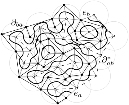
Figure 2: Construction of the diamond graph and the loop representation.

Critical weights for isoradial graphs

In the case of isoradial graphs, a natural family of weights can be defined. Let

$$x_{e}=\frac{p_{e}(1)}{(1-p_{e}(1))\sqrt{q}}=\frac{\sin[\frac{\sigma\theta_{e}}{2}]}{\sin[\frac{\sigma(\pi-\theta_{e})}{2}]}.$$

The bounded angle property immediately implies that weights are uniformly bounded away from 0 and 1.

This family of weights on isoradial graph is self-dual, in the sense that the dual of a random-cluster model with edge-weights ${\bf x}=(x_{e}:e\in\mathcal{E}[G])$ is a random cluster model on the (isoradial) dual graph with edge-weights $(x_{e^{*}}:e^{*}\in\mathcal{E}[G^{*}])$.

Let us stress out the fact that many other families of weights ${\bf x}$ are self-dual. Nevertheless, this family will play a special role for reasons that will become apparent later in the article.

Fix $\beta>0$. From now on, we will consider random-cluster measures

$$\phi_{G,\beta,q}^{\xi}(\{\omega\})=\phi_{G,\beta{\bf x},q}^{\xi}(\{\omega\})=\frac{1}{\tilde{Z}^{a,b}_{G,\beta{\bf x},q}}\Big{(}\prod_{e\in\omega}\beta x_{e}\Big{)}\sqrt{q}^{\#\;\text{loops}},$$

for any configuration $\omega$. Note that $(\phi^{0}_{G,\beta,q})^{*}=\phi^{1}_{G^{*},\beta^{-1},q}$.

Phase transition and critical point in the periodic case

In this paragraph, isoradial graphs are assumed to be periodic. We aim to study the behavior of $\phi^{\xi}_{G,\beta,q}$ when $\beta$ varies from $0$ to $\infty$. Positive association of the model implies that

$$\phi_{G,\beta,q}^{\xi}(A)\leq\phi^{\xi}_{G,\beta^{\prime},q}(A)$$

for any increasing event $A$ and $\beta\leq\beta^{\prime}$ (in such case, $\phi_{G,\beta,q}^{\xi}(A)$ is said to be stochastically dominated by $\phi_{G,\beta^{\prime},q}^{\xi}(A)$). The previous inequality extends to the infinite volume. It is therefore possible to define

$$\beta_{c}=\sup\{\beta\geq 0:\phi_{G_{\infty},\beta,q}^{0}(0\longleftrightarrow\infty)=0\},$$

where $0\longleftrightarrow\infty$ denotes the fact that 0 is contained in an infinite open path. This value is called the critical point.

We used $\phi_{G_{\infty},\beta,q}^{0}$ to define the critical point but the infinite-volume measure is not necessarily unique. Nevertheless, it can be shown that for a fixed $q\geq 1$ and a periodic isoradial graph $G_{\infty}$, uniqueness can fail only on a countable set $\mathcal{D}_{q,G_{\infty}}$. More precisely:

Proposition 8

Let $G_{\infty}$ be a periodic isoradial graph. There exists an at most countable set $\mathcal{D}_{q,G_{\infty}}\subset(0,\infty)$ such that for any $\beta\notin\mathcal{D}_{q,G_{\infty}}$, there exists a unique infinite-volume measure on $G_{\infty}$ with parameters $\beta$ and $q\geq 1$.

Proof

The proof follows the argument of [27, Theorem (4.63)] quite closely, so we only give a sketch here. Define the free energy per unit volume in a finite box as

$$H_{G}^{\xi}(\beta)=\frac{1}{|E[G]|}\log\tilde{Z}^{\xi}_{G,\beta,q}.$$

We have

$$\frac{\partial}{\partial\beta}H_{G}^{\xi}(\beta)=\frac{1}{|E[G]|}\sum_{e\in E[G]}x_{e}\phi^{\xi}_{G,\beta,q}(e\text{ is open})\in[0,\max\{x_{e}:e\in E[G_{\infty}]\}];$$

in particular, $H_{G}^{\xi}$ is convex. Now, let $G$ increase to cover the whole lattice. A classical argument of boundary-area energy comparison (see the lines following [27, Equation (4.71)]) shows that the limit $H(\beta)$ of $H_{G}^{\xi}(\beta)$ exists and does not depend on the boundary condition $\xi$.

Since $H$ is a uniform limit of convex functions, it is convex, and therefore differentiable outside an at most countable set $\mathcal{D}_{q,G_{\infty}}$. We may check that for any $\beta\notin\mathcal{D}_{q,G_{\infty}}$, both $\frac{\partial}{\partial\beta}H_{G}^{1}(\beta)$ and $\frac{\partial}{\partial\beta}H_{G}^{0}(\beta)$ converge to the same limit, which is also equal to $\frac{\partial}{\partial\beta}H(\beta)$. Hence, for any such $\beta$,

$$\lim_{G\nearrow G_{\infty}}\frac{1}{|E[G]|}\sum_{e\in E[G]}x_{e}\phi^{0}_{G,\beta,q}(e\text{ is open})=\lim_{G\nearrow G_{\infty}}\frac{1}{|E[G]|}\sum_{e\in E[G]}x_{e}\phi^{1}_{G,\beta,q}(e\text{ is open})$$

which is enough to guarantee that the measures $\phi_{G_{\infty},\beta,q}^{0}$ and $\phi_{G_{\infty},\beta,q}^{1}$ coincide; this in turn implies uniqueness of the Gibbs measure for all $\beta\notin\mathcal{D}_{q,G_{\infty}}$.   $\square$

Since the infinite-volume measure is unique for almost every $\beta$ (at fixed $q$), for any infinite-volume measure $\phi_{G_{\infty},\beta,q}$,

$$\phi_{G_{\infty},\beta,q}(0\longleftrightarrow\infty)\begin{cases}\ =0&\text{~{}if~{}}\beta<\beta_{c}\\ \ >0&\text{~{}if~{}}\beta>\beta_{c}\end{cases}.$$ (2.4)

Observables for Dobrushin domains

Fix a Dobrushin domain $(G,a,b)$ and consider the loop representation of the random-cluster model. Following [44], we now define an observable $F$ on the edges of its diamond graph, i.e. a function $F:\mathcal{E}[G^{\diamond}]\to\mathbb{R}_{+}$. Roughly speaking, $F$ is a modification of the probability that the exploration path passes through the center of an edge. First, we introduce the following definition: the winding $\text{W}_{\Gamma}(z,z^{\prime})$ of a curve $\Gamma$ between two edges $z$ and $z^{\prime}$ of the diamond graph is the total rotation (in radians) that the curve makes from the center of the diamond edge $z$ to the center of the diamond edge $z^{\prime}$.

Let $q>4$. We define the observable $F$ for any diamond edge $e\in\mathcal{E}[G^{\diamond}]$ by

$$F(e)=\phi_{G,\beta,q}^{a,b}\left({\rm e}^{\sigma\text{W}_{\gamma}(e,e_{b})}\mathbbm{1}_{e\in\gamma}\right),$$ (2.5)

where $\gamma$ is the exploration path and $\sigma>0$ is given by the relation

$$\cosh\big{(}\sigma\frac{\pi}{2}\big{)}=\frac{\sqrt{q}}{2}.$$ (2.6)

For $\sigma>0$ to exist, $q$ needs to be larger than $4$, hence the hypothesis in the theorem. We define the function $\tilde{F}$ by

$$\tilde{F}(e)=\phi_{G,\beta,q}^{a,b}\left({\rm e}^{-\sigma\text{W}_{\gamma}(e,e_{b})}\mathbbm{1}_{e\in\gamma}\right).$$ (2.7)

Remark 9

The observable $G(e)=\mathbb{E}_{G,a,b}\left({\rm e}^{{\rm i}\sigma\text{W}_{\gamma}(e,e_{b})}\mathbbm{1}_{e\in\gamma}\right)$, where $\sin(\sigma\pi/2)=\sqrt{q}/2$, was introduced in the case $q\leq 4$ in [44] for the square lattice. When weights are critical, one obtains around each vertex $v$

$$G(NW)-G(SE)={\rm i}[G(NE)-G(SW)],$$

where $NW$, $SE$, $NE$ and $SW$ are the your edges incident to $v$ indexed in the obvious way. This relation can be seen as a discrete version of the Cauchy-Riemann equation. The observable is then a holomorphic parafermion of spin $\sigma$ (which itself is a real number in $[0,1]$). For $q\geq 4$, $\sigma$ is purely imaginary and does not have an obvious physical meaning; it would nonetheless be interesting to find one. In this article, one could work with the corresponding $G$ for $q>4$, but the definitions in (2.5) and (2.7) are easier to handle for the applications we have in mind.

3 A representation formula for the observable

Let $(G,a,b)$ be a Dobrushin domain. In this section, we estimate the sum of $F$ over a set $E\subset\mathcal{E}[G^{\diamond}]$ in various ways. Let $\mathcal{F}^{\diamond}$ be the set of inner faces of $G^{\diamond}$. Any $f\in\mathcal{F}^{\diamond}$ is bordered by four edges in $\mathcal{E}[G^{\diamond}]$, which we label counterclockwise $A$, $B$, $C$ and $D$, so that locally the loops (or the exploration path) go from $f$ to the outside when crossing $A$ and $C$, and from the outside to $f$ when crossing $B$ and $D$; see Figure 3. There are a priori two ways to do so, but the choice will be irrelevant.

Lemma 10

Fix $\beta>0$ and $q>4$. For every face $f\in\mathcal{F}^{\diamond}$,

$$F(B)+F(D)=\Lambda_{e}(\beta x_{e})\left[F(A)+F(C)\right],$$ (3.1)

where $e$ is the edge of $G$ passing through $f$, and $\Lambda_{e}$ is given by $\displaystyle\Lambda_{e}(x)={\rm e}^{-\sigma(\pi-\theta_{e})}\frac{x+{\rm e}^{\sigma\frac{\pi}{2}}}{x+{\rm e}^{-\sigma\frac{\pi}{2}}}$.

A similar statement was used in [7] to derive massive harmonicity of the observable when $q=2$ on the square lattice. This enabled to compute the correlation length of the high temperature Ising model. Observe that $\Lambda(x_{e})=1$.

Proof

Consider the involution $s$ on the space of configurations which switches the state (open or closed) of the edge of $G$ passing through $f$.

Let $e$ be an edge of the diamond graph and denote by $e_{\omega}={\rm e}^{\sigma W_{\gamma}(e,e_{b})}\mathbbm{1}_{e\in\gamma}p(\omega)$ the contribution of $\omega$ to $F(e)$ (here $p(\omega)$ is the probability of the configuration $\omega$). Since $s$ is an involution, the following relation holds:

$$F(e)=\sum_{\omega}e_{\omega}=\textstyle\frac{1}{2}\displaystyle\sum_{\omega}\left[e_{\omega}+e_{s(\omega)}\right].$$

In order to prove (3.1), it suffices to prove the following for any configuration $\omega$:

$$B_{\omega}+B_{s(\omega)}+D_{\omega}+D_{s(\omega)}=\Lambda(\beta x_{e})\left[A_{\omega}+A_{s(\omega)}+C_{\omega}+C_{s(\omega)}\right].$$ (3.2)

When $\gamma(\omega)$ does not go through any of the diamond edges bordering $f$, neither does $\gamma(s(\omega))$. All the contributions then vanish and identity (3.2) trivially holds. Thus we may assume that $\gamma(\omega)$ passes through at least one edge bordering $f$. The interface enters $f$ through either $A$ or $C$ and leaves through $B$ or $D$. Without loss of generality, we assume that it enters first through $A$ and leaves last through $D$; the other cases are treated similarly.

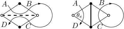
Figure 3: Two associated configurations $\omega$ and $s(\omega)$

Two cases can occur (see Figure 3): Either the exploration curve, after arriving through $A$, leaves through $B$ and then returns a second time through $C$, leaving through $D$; or the exploration curve arrives through $A$ and leaves through $D$, with $B$ and $C$ belonging to a loop. Since the involution exchanges the two cases, we can assume that $\omega$ corresponds to the first case. Knowing the term $A_{\omega}$, it is possible to compute the contributions of $\omega$ and $s(\omega)$ to all of the edges bordering $f$. Indeed,

• the probability of $s(\omega)$ is equal to $\beta x_{e}\sqrt{q}$ times the probability of $\omega$ (due to the fact that there is one additional loop, and the primal edge crossing $f$ is open);

• windings of the curve can be expressed using the winding of the edge $A$. For instance, the winding of $B$ in the configuration $\omega$ is equal to the winding of the edge $A$ plus an additional $-\theta_{e}$ turn.

Contributions are computed in the following table.

configuration	$A$	$B$	$C$	$D$
$\omega$	$A_{\omega}$	${\rm e}^{\sigma\theta_{e}}A_{\omega}$	${\rm e}^{-\sigma\pi}A_{\omega}$	${\rm e}^{-\sigma(\pi-\theta_{e})}A_{\omega}$
$s(\omega)$	$\beta x_{e}\sqrt{q}A_{\omega}$	0	0	${\rm e}^{-\sigma(\pi-\theta_{e})}\beta x_{e}\sqrt{q}A_{\omega}$

Using the identity ${\rm e}^{\sigma\frac{\pi}{2}}+{\rm e}^{-\sigma\frac{\pi}{2}}=\sqrt{q}$, we deduce (3.2) by summing the contributions of all the edges bordering $f$.   $\square$

For a set $E$ of edges of $\mathcal{E}[G^{\diamond}]$, $\partial_{\rm e}E$ denotes the set of edges of $\mathcal{E}[G^{\diamond}]\setminus E$ bordering the same face as an edge of $E$. Also define $E_{\rm int}$ to be the set of edges of the diamond graph between two faces of $\mathcal{F}^{\diamond}$.

Proposition 11

Fix $\beta<1$ and $q>4$. Let $G_{\infty}$ satisfying (BAP_θ). There exists $C_{1}=C_{1}(\beta,q,\theta)<\infty$ such that

$$\sum_{e\in E}F(e)\leq C_{1}\sum_{e\in\partial_{\rm e}E}F(e)$$

for any $E\subset E_{\rm int}$.

Proof

Sum the identity (3.1) over all faces bordered by an edge in $E$. It gives a weighted sum of $F(e)$ (with coefficients denoted by $c(e)$) which is identical to zero:

$$0=\sum_{e\in E}c(e)F(e)+\sum_{e\in\partial_{\rm e}E}c(e)F(e).$$ (3.3)

For an edge $e\in E$, $F(e)$ will appear in two such identities, corresponding to the two faces it borders. Since a loop going through $e$ comes from one of the faces and enters through the other one, the coefficients will be $-1$ and $\Lambda(\beta x_{e})$. Thus, for $e\in E$, $F(e)$ enters the sum with a coefficient

$$c(e)=\Lambda(\beta x_{e})-1 ={\rm e}^{-\sigma(\pi-\theta_{e})}\left(\frac{\beta x_{e}+{\rm e}^{\sigma\frac{\pi}{2}}}{\beta x_{e}+{\rm e}^{-\sigma\frac{\pi}{2}}}\right)-1=\left(\frac{x_{e}+{\rm e}^{-\sigma\frac{\pi}{2}}}{x_{e}+{\rm e}^{\sigma\frac{\pi}{2}}}\right)\left(\frac{\beta x_{e}+{\rm e}^{\sigma\frac{\pi}{2}}}{\beta x_{e}+{\rm e}^{-\sigma\frac{\pi}{2}}}\right)-1$$

$$=\left(1+\frac{(\beta-1)x_{e}}{x_{e}+{\rm e}^{\sigma\frac{\pi}{2}}}\right)\left(1-\frac{(\beta-1)x_{e}}{\beta x_{e}+{\rm e}^{-\sigma\frac{\pi}{2}}}\right)-1$$

$$=(\beta-1)x_{e}\left(\frac{{\rm e}^{-\sigma\frac{\pi}{2}}-{\rm e}^{\sigma\frac{\pi}{2}}}{(x_{e}+{\rm e}^{\sigma\frac{\pi}{2}})(\beta x_{e}+{\rm e}^{-\sigma\frac{\pi}{2}})}\right)=\frac{2(1-\beta)x_{e}\sinh(\textstyle\sigma\frac{\pi}{2})}{(x_{e}+{\rm e}^{\sigma\frac{\pi}{2}})(\beta x_{e}+{\rm e}^{-\sigma\frac{\pi}{2}})}$$

$$\geq 2(1-\beta)\,\min\big{\{}x_{e}:e\in\mathcal{E}[G]\big{\}}\,\sinh(\textstyle\sigma\frac{\pi}{2}).$$

In the second equality, we used that $\Lambda(x_{e})=1$. Because of the bounded angle property, $x_{e}$ is bounded away from 0 and $\infty$ uniformly, and so is $c(e)$.

For an edge $e\in\partial_{\rm e}E$, $F(e)$ will appear in exactly one identity, (corresponding to the face that it shares with an edge of $E$). The coefficient will be $\Lambda(\beta x_{e})$ or $-1$, depending on the orientation of $e$ with respect to the face. Thus $F(e)$ will enter the sum with a coefficient $c(e)$ which is bounded from above uniformly in $e$ (thanks to the Bounded Angle Property). The proposition follows immediately by setting

$$C_{1}=C_{1}(\beta,q,\theta):=\frac{\max\{|c(e)|:e\in\partial_{\rm e}E\}}{\min\{|c(e)|:e\in E\}}=\frac{\max\{|c(e)|:e\in E[G_{\infty}^{\diamond}]\}}{\min\{|c(e)|:e\in E[G_{\infty}^{\diamond}]\}}<0.$$

Note that $C_{1}$ depends only on $\beta$, $q$ and $\theta$, but not on $G_{\infty}$ or $E$.   $\square$

Write $\partial\mathcal{E}[G^{\diamond}]$ for the edge-boundary of $G^{\diamond}$, meaning the set of diamond edges connecting two boundary vertices. Note that it is simply $E[G^{\diamond}]\setminus E_{\rm int}$.

Lemma 12

Let $(G,a,b)$ be a Dobrushin domain. For a site $u$ on the free arc $\partial_{ab}$ and $e\in\partial\mathcal{E}[G^{\diamond}]$ a diamond edge incident to $u$, we have

$$F(e)~{}=~{}{\rm e}^{\sigma W(e,e_{b})}\cdot\phi_{G,\beta,q}^{a,b}(u\leftrightarrow\text{wired arc }\partial_{ba}),$$

where $W(e,e_{b})$ is the winding of an arbitrary curve on the diamond graph from $e$ to $e_{b}$.

Proof

Let $u$ be a site of the free arc $\partial_{ab}$ and recall that the exploration path is the interface between the open cluster connected to the wired arc and the dual open cluster connected to the free arc. Since $u$ belongs to the free arc, $u$ is connected to the wired arc if and only if $e$ belongs to the exploration path, so that

$$\phi_{G,\beta,q}^{a,b}(u\leftrightarrow\text{wired arc }\partial_{ba})=\phi_{G,\beta,q}^{a,b}(e\in\gamma).$$

The edge $e$ being on the boundary, the exploration path cannot wind around it, so that the winding of the curve is deterministic. Call this winding $W(e,e_{b})$. We deduce from this remark that

$$F(e)=\phi_{G,\beta,q}^{a,b}({\rm e}^{\sigma W_{\gamma}(e,e_{b})}\mathbbm{1}_{e\in\gamma}) ={\rm e}^{\sigma W(e,e_{b})}\phi_{G,\beta,q}^{a,b}(e\in\gamma)={\rm e}^{\sigma W(e,e_{b})}\phi_{G,\beta,q}^{a,b}(u\leftrightarrow\text{wired arc }\partial_{ba}).$$

$\square$

We are now in a position to prove our key proposition.

Proposition 13

Fix $q>4$ and $G_{\infty}$ satisfying (BAP_θ). There exists $C_{2}=C_{2}(q,\theta)<\infty$ such that

$$\sum_{e\in\partial\mathcal{E}[G^{\diamond}]}F(e)\leq C_{2}{\rm e}^{\sigma(W_{\rm max}-W_{\rm min})}$$

for any $\beta\leq 1$ and any Dobrushin domain $(G,0,0)$ (here, $0$ is assumed to belong to $\partial G$). Above, $W_{\rm min}$ and $W_{\rm max}$ are the minimal and maximal winding when going along the boundary of $G$, starting from $0$.

Note that Dobrushin boundary conditions on $(G,0,0)$ coincide with free boundary conditions.

Proof

Let us start with the case $\beta=1$. Sum Identity (3.1) over all $\mathcal{F}^{\diamond}$. Since $\Lambda(x_{e})=1$ for any $e$, we find that $c(e)=0$ for any $e\in E_{\rm int}$ and $c(e)=\pm 1$ on $\partial E[G^{\diamond}]$ depending on the fact that a loop going through $e$ points outwards or inward $\mathcal{F}^{\diamond}$. Boundary edges corresponding to a loop pointing outward are called exiting, those for which the loop is pointing inward entering. We find

$$\sum_{e\text{~{}exiting}}F(e)~{}-\sum_{e\text{~{}entering}}F(e)=0.$$

Since edges exiting or entering belong to $\partial\mathcal{E}[G^{\diamond}]$, Lemma 12 implies that

$$F(e)={\rm e}^{\sigma W(e,e_{b})}\phi^{0}_{G,1,q}[u\longleftrightarrow 0],$$

for $u$ the site of $G$ bordering $e$. Note that each vertex $u\in\partial G$ is the end-point of a unique entering edge, called $e_{\rm in}(u)$ and a unique exiting edge $e_{\rm ex}(u)$. With this definition and the two previous displayed equalities, we find

$$\sum_{u\in\partial G}\left[{\rm e}^{\sigma W(e_{\rm ex}(u),e_{b})}-{\rm e}^{\sigma W(e_{\rm in}(u),e_{b})}\right]\phi^{0}_{G,1,q}(u\longleftrightarrow 0)=0$$

which can be rewritten as

$$\sum_{u\in\partial G\setminus\{0\}}\left[{\rm e}^{\sigma W(e_{\rm ex}(u),e_{b})}-{\rm e}^{\sigma W(e_{\rm in}(u),e_{b})}\right]\phi^{0}_{G,1,q}(u\longleftrightarrow 0)={\rm e}^{\sigma W(e_{\rm in}(0),e_{b})}-{\rm e}^{\sigma W(e_{\rm ex}(0),e_{b})}.$$

Now, when $u=0$, $e_{\rm in}(0)=e_{a}$ and $e_{\rm ex}(0)=e_{b}$. Since $W(e_{a},e_{b})\leq 2\pi$,

$${\rm e}^{\sigma W(e_{\rm in}(0),e_{b})}-{\rm e}^{\sigma W(e_{\rm ex}(0),e_{b})}={\rm e}^{\sigma W(e_{a},e_{b})}-{\rm e}^{\sigma W(e_{b},e_{b})}\leq{\rm e}^{\sigma 2\pi}.$$

When $u\neq 0$, we find that

$$W(e_{\rm ex}(u),e_{b})-W(e_{\rm in}(u),e_{b})=W(e_{\rm ex}(u),e_{\rm in}(u))\geq\theta_{[uv]}\geq\theta,$$

where $v$ is a neighbor of $u$ outside of $G$, and $[uv]$ is the edge between $u$ and $v$. Note that the existence of this neighbor is guaranteed by the fact that $u\in\partial G$. Next,

$${\rm e}^{\sigma W(e_{\rm ex}(u),e_{b})}-{\rm e}^{\sigma W(e_{\rm in}(u),e_{b})}=\left[{\rm e}^{\sigma W(e_{\rm ex}(u),e_{\rm in}(u))}-1\right]{\rm e}^{\sigma W(e_{\rm in}(u),e_{b})}\geq[{\rm e}^{\sigma\theta}-1]{\rm e}^{\sigma W_{\rm min}}.$$

Therefore,

$$[{\rm e}^{\sigma\theta}-1]{\rm e}^{\sigma W_{\rm min}}\sum_{u\in\partial G\setminus\{0\}}\phi^{0}_{G,1,q}(u\longleftrightarrow 0)\leq{\rm e}^{\sigma 2\pi}.$$

Finally, observe that

$$\sum_{e\in\partial\mathcal{E}[G^{\diamond}]}F(e) =\sum_{e\in\partial\mathcal{E}[G^{\diamond}]}{\rm e}^{\sigma W(e,e_{b})}\phi^{0}_{G,1,q}[u\longleftrightarrow 0]$$

$$\leq 4{\rm e}^{\sigma W_{\rm max}}\sum_{u\in\partial G}\phi^{0}_{G,1,q}[u\longleftrightarrow 0]\leq 4{\rm e}^{\sigma W_{\rm max}}+4{\rm e}^{\sigma W_{\rm max}}\sum_{u\in\partial G\setminus\{0\}}\phi^{0}_{G,1,q}[u\longleftrightarrow 0]$$

$$\leq 4{\rm e}^{\sigma W_{\rm max}}+4\frac{{\rm e}^{\sigma(W_{\rm max}-W_{\rm min})}}{{\rm e}^{\sigma\theta}-1}{\rm e}^{\sigma 2\pi}.$$

In the first inequality, we used the fact that at most four edges correspond to a boundary vertex.

The case $\beta\leq 1$ follows readily since $F(e)={\rm e}^{\sigma W(e,e_{b})}\phi^{0}_{G,\beta,q}[u\longleftrightarrow 0]$ is an increasing quantity in $\beta$.   $\square$

For a graph $G$, let us introduce the following, recursively constructed graphs. Let $G^{(0)}=G$ and $G^{(k)}=G^{(k-1)}\setminus\partial G^{(k-1)}$ for any $k\geq 1$. They can be seen as successive “pealings” of $G$, each step consisting in removing the boundary of the existing graph. Let $E_{k}=E_{\rm int}[G^{(k)}]$. Note that $E_{0}=E_{\rm int}=\mathcal{E}[G^{\diamond}]\setminus\partial\mathcal{E}[G^{\diamond}]$.

Corollary 14

Let $G_{\infty}$ be an isoradial graph satisfying (BAP_θ). Consider the Dobrushin domain $(G,0,0)$ (as above, $0$ is assumed to be on the boundary of $G$). For any $\beta<1$ and $q>4$,

$$\sum_{e\in E_{k}}F(e)\leq C_{1}C_{2}{\rm e}^{\sigma(W_{\rm max}-W_{\rm min})}\left(\frac{C_{1}}{1+C_{1}}\right)^{k}.$$

Proof

Proposition 11 can be applied to $E_{k}\subset E_{\rm int}$ to give

$$\sum_{e\in E_{k}}F(e)\leq\frac{C_{1}}{1+C_{1}}\sum_{e\in E_{k}\cup\partial_{\rm e}E_{k}}F(e).$$

Since $E_{k}\cup\partial_{\rm e}E_{k}\subset E_{k-1}$ and $F(e)\geq 0$,

$$\sum_{e\in E_{k}}F(e)\leq\frac{C_{1}}{1+C_{1}}\sum_{e\in E_{k-1}}F(e).$$

Using the previous bound iteratively, and Proposition 11 one last time (in the second inequality), we find

$$\sum_{e\in E_{k}}F(e) \leq\left(\frac{C_{1}}{1+C_{1}}\right)^{k}\sum_{e\in E_{\rm int}}F(e)\leq C_{1}\left(\frac{C_{1}}{1+C_{1}}\right)^{k}\sum_{e\in\partial\mathcal{E}[G^{\diamond}]}F(e)$$

The claim follows by bounding the sum on the right-hand side using Proposition 13.   $\square$

The study above can be performed with $\tilde{F}$ instead of $F$. We obtain the following corollary.

Corollary 15

Let $G_{\infty}$ satisfying (BAP_θ). Consider the Dobrushin domain $(G,0,0)$ ($0$ is assumed to be on the boundary of $G$). For any $\beta<1$ and $q>4$,

$$\sum_{e\in E_{k}}\tilde{F}(e)\leq C_{1}C_{2}{\rm e}^{\sigma(W_{\rm max}-W_{\rm min})}\left(\frac{C_{1}}{1+C_{1}}\right)^{k}.$$

4 Proof of Theorem 2

Without loss of generality, we assume that $v=0$. Fix $\beta<1$. We aim to prove that there exists $c=c(\beta,q,\theta)>0$ such that

$$\phi^{0}_{G_{\infty},\beta,q}(0\longleftrightarrow u)\leq\exp(-c|u|)$$

for any $u\in G_{\infty}$ containing $0$. We now fix $G_{\infty}$ containing 0 and satisfying (BAP_θ). We stress out that the constants involved in the proof depend on $\theta$ only but not on $G_{\infty}$ or $u$.

The case $q=4$ is derived through stochastic domination between random cluster measures. Indeed, for every $\beta<1$, there exists $(\beta^{\prime},q)$ with $q>4$ and $\beta^{\prime}<1$ such that the random-cluster measure $\phi^{0}_{G_{\infty},\beta^{\prime},q}$ stochastically dominates the random-cluster measure $\phi^{0}_{G_{\infty},\beta,4}$. We refer to [27, Theorem (3.23)] for details on this fact. It follows from this stochastic domination that

$$\phi^{0}_{G_{\infty},\beta,4}(0\longleftrightarrow u)\leq\phi^{0}_{G_{\infty},\beta^{\prime},q}(0\longleftrightarrow u)\leq\exp\big{[}-c(\beta^{\prime},q,\theta)|u|\big{]}$$

for any $u\in G_{\infty}$. It is therefore sufficient to assume that $q>4$, which we now do.

For a graph $G_{\infty}$, we identify a convex subset $A$ of $\mathbb{R}^{2}$ with the subgraph given by vertices in $G_{\infty}\cap A$ and edges between them. The set $\partial A$ is referring to $\partial(G_{\infty}\cap A)$. Note that this set is not necessarily connected, but this will not be relevant in the following. For $r>0$, let $B_{0}(r)=\{x\in\mathbb{R}^{2}:|x|<r\}$.

Lemma 16

There exists $c_{1}=c_{1}(\beta,q,\theta)>0$. Assume that $v\in G_{\infty}$ is on the positive real axis. Then,

$$\phi^{0}_{[0,\infty)\times(-\infty,\infty),\beta,q}(0\longleftrightarrow v)\leq\exp[-c_{1}|v|].$$

There could be no vertex $v$ on the positive axis, but there is no loss of generality in assuming that $v$ belongs to this positive axis, since the graph $G_{\infty}$ can be rotated around the origin in order to obtain an estimate valid for any vertex $v\in G_{\infty}$, where the half-plane $[0,\infty)\times(-\infty,\infty)$ is replaced by a half-plane containing $v$ whose boundary contains 0 and is orthogonal to the vector given by the coordinates of $v$.

Proof

Define $G_{m,n}$ to be the connected component of the origin in $[0,n]\times[-m,m]$. Set $k=|v|/2$. Let $m\geq 100$ and $n>\max\{2|v|,100\}$ (these two conditions avoid nasty local problems). Apply Corollaries 14 and 15 to $G_{m,n}$ and $k$ to find (we use the notation of the corollary)

$$\sum_{e\in E_{k}}F(e)+\tilde{F}(e)\leq 2C_{1}C_{2}{\rm e}^{\sigma(W_{\rm max}-W_{\rm min})}\left(\frac{C_{1}}{1+C_{1}}\right)^{k}.$$

The maximum and minimum windings on $\partial E[G_{m,n}]$ are bounded by a certain constant $C_{3}<\infty$. This statement comes from the fact that the winding of $\partial E[G_{m,n}]$ is roughly comparable of the winding of the boundary of $[0,n]\times[-m,m]$ (there are a few local effects to take care of). Let us sketch an argument. There exists a path of adjacent faces of the subgraph $H_{m,n}=[0,n]\times[-m,m]\setminus[4,n-4]\times[-m+4,m-4]$ of $G_{m,n}$ going around $[4,n-4]\times[-m+4,m-4]$. The constant 4 has been chosen to fit our purpose. It can probably be improved but this would be of no interest for the proof. In particular, $\partial E[G_{m,n}]$ is contained in $H_{m,n}$. The bounded angle property shows that two vertices cannot be arbitrary close to each other, which prevents the existence of paths of edges in $E[H_{m,n}]$ winding arbitrary often around a point of $\mathbb{R}^{2}$. As a consequence, the winding along $\partial E[G_{m,n}]$ is indeed bounded by a universal constant.

The previous bounds on $W_{\rm max}$ and $W_{\rm min}$ imply

$$\sum_{e\in E_{k}}F(e)+\tilde{F}(e)\leq C_{4}\left(\frac{C_{1}}{1+C_{1}}\right)^{k}.$$

Next, observe that

$$F(e)+\tilde{F}(e)=\phi^{0}_{G_{m,n},\beta,q}\left[({\rm e}^{\sigma W(e,e_{b})}+{\rm e}^{-\sigma W(e,e_{b})})\mathbbm{1}_{e\in\gamma}\right]\geq 2\phi^{0}_{G_{m,n},\beta,q}(e\in\gamma).$$

Let $\mathcal{C}_{0}$ be the cluster of the origin and $\partial_{\rm out}\mathcal{C}_{0}$ its outer boundary, meaning the set of vertices connected to the free arc by a path in $E[G_{\infty}]\setminus E[\mathcal{C}_{0}]$. A diamond edge $e=[vy]$, where $v\in G_{m,n}$ and $y\in G_{m,n}^{*}$ belongs to $\gamma$ if and only if 0 is connected to $v$ and $y$ is connected to the free arc. In other words, $v$ is on the outer boundary of the cluster of 0. We deduce that

$$\phi^{0}_{G_{m,n},\beta,q}(\partial_{\rm out}\mathcal{C}_{0}\cap G_{m,n}^{(k)}\neq\emptyset) \leq\sum_{u\in G_{m,n}^{(k)}}\phi^{0}_{G_{m,n},\beta,q}(u\in\partial\mathcal{C}_{0})$$

$$\leq\sum_{e\in E_{\rm int}^{(k-1)}}F(e)+\tilde{F}(e)$$

$$\leq C_{4}\left(\frac{C_{1}}{1+C_{1}}\right)^{k-1}.$$

Letting $m$ go to infinity and using the uniform bound above,

$$\phi^{0}_{G_{\infty,n},\beta,q}(\partial_{\rm out}\mathcal{C}_{0}\cap G_{\infty,n}^{(k)}\neq\emptyset)\leq C_{5}\left(\frac{C_{1}}{1+C_{1}}\right)^{k},$$

where $G_{\infty,n}=[0,n]\times(-\infty,\infty)$. Next, observe that $G_{\infty,n}$ does not contain any infinite cluster $\phi_{G_{\infty,n},\beta,q}$-almost surely (in fact, this is true for any $\beta^{\prime}<\infty$, since the graph is rough isometric to $\mathbb{Z}$). Let us provide a rigorous proof of this statement. The experienced reader can skip the next paragraph.

The bounded angle condition implies that the weight $x_{e}$ is bounded from above uniformly on $G_{\infty}$. Therefore, there exits $c_{2}=c_{2}(\beta,q,\theta)>0$ such that for any finite set $S$ of dual edges of cardinality $r$

$$\phi^{0}_{G_{\infty,n},\beta,q}(\text{every edge in $S$ is dual-open}~{}|~{}\mathcal{F}_{\mathcal{E}[G_{\infty,n}^{*}]\setminus S})\geq\exp[-c_{2}r].$$

The constant $c_{2}$ comes from the finite-energy of the random-cluster model, i.e. the property that the probability for an edge to be closed is bounded away from 0 uniformly in the state of all the other edges; see [27, Equation (3.4)]. Next, it is possible to divide the strip into an infinite number of finite pieces by considering disconnecting paths $P$ of length less than $c_{3}n$ for some constant $c_{3}=c_{3}(\theta)<\infty$. The existence of these paths is easily proved by considering a sequence of set of adjacent faces cutting the strip, and by noticing that the bounded angle property bounds from above the number of edges bordering a face by $\pi/\sin(\theta/2)$. Now, conditioned on the state of the others paths, each one of these paths has probability larger than $\exp[-c_{2}c_{3}n]>0$ of being dual-open. This immediately implies that there is no infinite cluster $\phi_{G_{\infty,n},\beta,q}$-almost surely.

Since there is no infinite cluster almost surely, $\mathcal{C}_{0}$ intersects $G_{\infty,n}^{(k)}$ if and only if $\partial_{\rm out}\mathcal{C}_{0}$ intersects $G_{\infty,n}^{(k)}$. Furthermore, edges have length smaller than 2, which implies that $u\in G_{\infty,n}^{(k)}$ (we use the fact that $n-|v|$ and $|v|$ are larger than $2k$). Hence,

$$\phi^{0}_{G_{\infty,n},\beta,q}(0\longleftrightarrow v)\leq\phi^{0}_{G_{\infty,n},\beta,q}(\mathcal{C}_{0}\cap G_{\infty,n}^{(k)}\neq\emptyset)=\phi^{0}_{G_{\infty,n},\beta,q}(\partial\mathcal{C}_{0}\cap G_{\infty,n}^{(k)}\neq\emptyset)\leq C_{5}\left(\frac{C_{1}}{1+C_{1}}\right)^{k}.$$

The proof follows by letting $n$ go to infinity and then by choosing $c_{1}=c_{1}(\beta,q,\theta)>0$ small enough.   $\square$

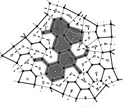
Figure 4: The gray area is $\overline{\gamma}$. The dual path surrounding it is $\Gamma$. It is the exterior-most dual circuit.

We are now in a position to prove Theorem 2. Let $n>|u|+2$. We work with the random-cluster measure on $B_{0}(n)$ with free boundary conditions. Let $X_{\rm max}$ be the site of $B_{0}(n)\cap\mathcal{C}_{0}$ which maximizes its Euclidean distance to the origin (when several such sites exist, take the first one for an arbitrary indexation of sites in $G_{\infty}$). Note that $|u|\leq|X_{\rm max}|<n$. Therefore,

$$\phi^{0}_{B_{0}(n),\beta,q}(0\longleftrightarrow u) \leq\phi^{0}_{B_{0}(n),\beta,q}(\exists v\in B_{0}(n)\setminus B_{0}(|u|):X_{\rm max}=v)$$

$$\leq\sum_{v\in B_{0}(n)\setminus B_{0}(|u|)}\phi^{0}_{B_{0}(n),\beta,q}(X_{\rm max}=v).$$ (4.1)

For $v$, let $\mathfrak{C}(v)$ be the set of dual-open self-avoiding circuits $\gamma$ surrounding the origin and $v$ and such that any site of $B_{0}(n)$ surrounded by $\gamma$ is in $B_{0}(|v|)$. Let $\overline{\gamma}$ be the set of sites of $B_{0}(n)$ surrounded by $\gamma\in\mathfrak{C}(v)$, see Fig. 4. Dual-open circuits in $\mathfrak{C}(v)$ are naturally ordered via the following order relation: $\gamma$ is more exterior than $\gamma^{\prime}$ if $\overline{\gamma}\subset\overline{\gamma}^{\prime}$.

If $X_{\rm max}=v$, then $v$ is connected to $0$ and there exists a circuit in $\mathfrak{C}(v)$ which is dual-open (simply take the boundary of $\mathcal{C}_{0}$, drawn on the dual graph). Let $\{\Gamma=\gamma\}$ be the event that $\gamma$ is the exterior-most dual-open circuit in $\mathfrak{C}(v)$. With this definition, $X_{\rm max}=v$ if and only if $v$ is connected to 0 and there exists $\gamma\in\mathfrak{C}(v)$ such that $\Gamma=\gamma$. Therefore

$$\phi^{0}_{B_{0}(n),\beta,q}(X_{\rm max}=v) =\phi^{0}_{B_{0}(n),\beta,q}(0\longleftrightarrow v\text{~{}and~{}}\exists\gamma\in\mathfrak{C}(v):\Gamma=\gamma)$$

$$=\sum_{\gamma\in\mathfrak{C}(v)}\phi^{0}_{B_{0}(n),\beta,q}(0\longleftrightarrow v\text{~{}and~{}}\Gamma=\gamma)$$

$$=\sum_{\gamma\in\mathfrak{C}(v)}\phi^{0}_{B_{0}(n),\beta,q}(0\longleftrightarrow v|\Gamma=\gamma)\phi^{0}_{B_{0}(n),\beta,q}(\Gamma=\gamma)$$

Since $\Gamma$ is the exterior most circuit in $\mathfrak{C}(v)$, $\{\Gamma=\gamma\}$ is measurable with respect to dual-edges outside $\gamma$. Furthermore, edges of $\gamma$ are dual-open on $\{\Gamma=\gamma\}$, see Fig. 4. Therefore, conditioned on $\{\Gamma=\gamma\}$, the measure inside $\overline{\gamma}$ is a random-cluster model with free boundary conditions. Hence,

$$\phi^{0}_{B_{0}(n),\beta,q}(0\longleftrightarrow v|\Gamma=\gamma)=\phi^{0}_{\overline{\gamma},\beta,q}(0\longleftrightarrow v).$$

Rotate the graph $B_{0}(n)$ in such a way that $v$ is on the positive axis. Let $H=(-\infty,v]\times\mathbb{R}$. Observe that by definition of $\mathfrak{C}(v)$, $\overline{\gamma}\subset H$. The comparison between boundary conditions leads to

$$\phi^{0}_{\overline{\gamma},\beta,q}(0\longleftrightarrow v)\leq\phi^{0}_{H,\beta,q}(0\longleftrightarrow v\text{ in }\overline{\gamma})\leq\phi^{0}_{H,\beta,q}(0\longleftrightarrow v)\leq\exp[-c_{1}|v|]$$

by Lemma 16. This implies

$$\phi^{0}_{B_{0}(n),\beta,q}(X_{\rm max}=v)\leq\sum_{\gamma\in\mathfrak{C}(y)}\exp[-c_{1}|v|]\phi^{0}_{B_{0}(n),\beta,q}(\Gamma=\gamma)\leq\exp[-c_{1}|v|].$$

In the second equality, we used the fact that the union of $\{\Gamma=\gamma\}$ for $\gamma\in\mathfrak{C}(v)$ is disjoint. Going back to (4.1), we find

$$\phi^{0}_{B_{0}(n),\beta,q}(0\longleftrightarrow u) \leq\sum_{v\in B_{0}(n)\setminus B_{0}(|u|)}\exp[-c_{1}|v|]$$

$$\leq\sum_{v\in G_{\infty}\setminus B_{0}(|u|)}\exp[-c_{1}|v|]$$

$$\leq\sum_{k\geq 0}|B_{0}(|u|+k+1)\setminus B_{0}(|u|+k)|\exp[-c_{1}(|u|+k)]$$

$$\leq\sum_{k\geq 0}|\textstyle\frac{\pi}{\sin(\theta/2)}(|u|+k+1)|\displaystyle\exp[-c_{1}(|u|+k)]$$

$$\leq c_{4}|u|\exp[-c_{1}|u|].$$

In the fourth inequality, we used the fact that the number of sites in $B_{0}(r+1)\setminus B_{0}(r)$ is bounded by $\frac{\pi}{\sin(\theta/2)}(r+1)$ because of the bounded angle property.

The proof follows by letting $n$ go to infinity and by choosing $c=c(\beta,q,\theta)>0$ small enough.

Remark 17

The main point of the previous proofs, and of our whole approach, is that the observable $F$ behaves like a massive-harmonic function. We are not able to make exact computations though, because we made no particular effort to choose our coupling constants with this goal in mind (all that matters here is that the constant $C_{1}$ is bounded). In a recent work [9], Boutillier, de Tilière and Raschel define a massive Laplacian operator on isoradial graphs for which they get the explicit rate of exponential decay of massive-harmonic functions. It would be interesting to see whether a better tuned choice of the $p_{e}(\beta)$ can lead to an exactly massive-harmonic observable in their sense, as this would lead to sharper asymptotics for the two-point function of the model in that case.

5 Proofs of the remaining theorems and corollaries

Proof of Theorem 4

Fix $\beta<1$. Let $G_{\infty}$ be an infinite isoradial graph. Without loss of generality (simply translate the graph), we assume that $y=0\in G_{\infty}$. For $r>0$, Theorem 2 implies

$$\phi^{0}_{G_{\infty},\beta,q}(0\longleftrightarrow\partial B_{0}(r)) \leq\sum_{u\in\partial B_{0}(r)}\phi^{0}_{G_{\infty},\beta,q}(0\longleftrightarrow u)$$

$$\leq\frac{\pi r^{2}}{4\sin(\theta/2)}\exp\big{[}-c(\beta,q,\theta)(r-2)\big{]}.$$ (5.1)

In the second inequality, we used the fact that any site $u\in\partial B_{0}(r)$ is at distance larger than $r-2$ of the origin since any primal edge is of length smaller than 2 (the diameter of circles is 2), and that $u\in\partial B_{0}(r)$ is connected to a site outside $B_{0}(r)$. We also used the fact that the cardinality of $B_{0}(r)$ is smaller than $\pi r^{2}/(4\sin(\theta/2))$ since any edge of $G_{\infty}$ corresponds to a face of $G_{\infty}^{\diamond}$ of volume larger than $4\sin(\theta/2)$ thanks to the bounded angle property. Letting $r$ go to infinity, we obtain that $\phi^{0}_{G_{\infty},\beta,q}(0\longleftrightarrow\infty)=0$.

Let us now consider $\phi^{1}_{G,\beta,q}$ with $\beta>1$. For a dual vertex $y\in G^{*}$, let $A(y)$ be the event that there exists a dual-open circuit surrounding the origin, i.e.  a path of dual-open edges disconnecting $0$ from infinity in $\mathbb{R}^{2}$. Observe that the dual circuit must go to distance $|y|$. Since the dual model is a random-cluster model on the dual isoradial graph, with free boundary conditions and with $\beta^{*}=1/\beta<1$, (5.1) implies

$$\phi^{1}_{G_{\infty},\beta,q}(A(y))\leq\frac{\pi|y|^{2}}{4\sin(\theta/2)}\exp\big{[}-c(1/\beta,q,\theta)(|y|-2)\big{]}$$

for any $y\in G_{\infty}^{*}$. Borel-Cantelli lemma together with the bound $|G_{\infty}^{*}\cap B_{0}(r)|\leq\frac{\pi r^{2}}{4\sin(\theta/2)}$ implies that

$$\phi^{1}_{G_{\infty},\beta,q}(\text{there exist infinitely many }y\in G_{\infty}^{*}:A(y))=0.$$

This immediately implies that there exists an infinite cluster $\phi^{1}_{G_{\infty},\beta,q}$-almost surely.   $\square$

Proof of Theorem 3

Let us now turn to the uniqueness question. This is the only place where a priori information on uniqueness is used. Recall that in this case, $\mathcal{D}_{G_{\infty},q}$ defined in Proposition 8 is countable. Since $\phi^{0}_{G_{\infty},\beta,q}=\phi^{1}_{G_{\infty},\beta,q}$ outside of the countable set $\mathcal{D}_{G_{\infty},q}$, for any $\beta<1$ there exists $\beta<\beta^{\prime}<1$ such that $\phi^{1}_{G_{\infty},\beta^{\prime},q}=\phi^{0}_{G_{\infty},\beta^{\prime},q}$. We deduce that

$$\phi^{1}_{G_{\infty},\beta,q}(0\longleftrightarrow\infty)\leq\phi^{1}_{G_{\infty},\beta^{\prime},q}(0\longleftrightarrow\infty)=\phi^{0}_{G_{\infty},\beta^{\prime},q}(0\longleftrightarrow\infty)=0.$$

From [27, Theorem (5.33)], we deduce that $\phi^{1}_{G_{\infty},\beta,q}=\phi^{0}_{G_{\infty},\beta,q}$ for any $\beta<1$. Theorem (5.33) is proved in the case of $\mathbb{Z}^{d}$, but the proof extends to the context of periodic graphs mutatis mutandis. By duality, the infinite-volume measure is unique except possibly for $\beta=1$. This implies in particular that there is $\phi^{0}_{G_{\infty},\beta,q}$-almost surely an infinite cluster whenever $\beta>1$.   $\square$

Proof of Corollary 5

We present the proof in the case of the square lattice, the cases of triangular and hexagonal lattices being the same. If $\frac{p_{1}}{1-p_{1}}\frac{p_{2}}{1-p_{2}}=\beta q$, then $x_{1}x_{2}=1$ where $x_{i}=\frac{p_{i}}{(1-p_{i})\sqrt{q\beta}}$. By embedding the square lattice in such a way that every face is a rectangle inscribed in a circle of radius 1, and the aspect ratio is given by $x_{1}/x_{2}$, we obtain an isoradial graph with critical weights $x_{1}$ and $x_{2}$. The model is therefore subcritical (respectively supercritical) if and only if $\beta<1$ (respectively $\beta>1$).   $\square$

Proof of Corollary 6

Corollary 6 follows directly from the classical coupling between random-cluster models and Potts models.   $\square$

Acknowledgments.

This work has been accomplished during the stay of the first author in Geneva. The authors were supported by the ANR grant 10-BLAN-0123, the EU Marie-Curie RTN CODY, the ERC AG CONFRA, the NCCR SwissMap founded by the Swiss NSF, as well as by the another grant from the Swiss NSF. The authors would like to thank Geoffrey Grimmett for many fruitful discussions.

References

- [1] R. J. Baxter, Solvable eight-vertex model on an arbitrary planar lattice, Philos. Trans. Roy. Soc. London Ser. A, 289 (1978), pp. 315–346.
- [2] , Exactly solved models in statistical mechanics, Academic Press Inc. [Harcourt Brace Jovanovich Publishers], London, 1989. Reprint of the 1982 original.
- [3] N. Beaton, M. Bousquet-Mélou, H. Duminil-Copin, J. de Gier, and A. J. Guttmann, The critical fugacity for surface adsorption of self-avoiding walks on the honeycomb lattice is , Comm. Math. Phys, 326 (2014), pp. 727–754.
- [4] N. Beaton, A. J. Guttmann, and I. Jensen, A numerical adaptation of SAW identities from the honeycomb to other 2D lattices, J. Phys. A: Math. Theor., 45 (2012), p. 035201.
- [5] , Two-dimensional self-avoiding walks and polymer adsorption: Critical fugacity estimates, J. Phys. A: Math. Theor., 45 (2012), p. 055208.
- [6] V. Beffara and H. Duminil-Copin, The self-dual point of the two-dimensional random-cluster model is critical for , Prob. Theory Related Fields, 153 (2012), pp. 511–542.
- [7] , Smirnov’s fermionic observable away from criticality, Ann. Probab., 40 (2012), pp. 2667–2689.
- [8] S. Benoist, H. Duminil-Copin, and C. Hongler, Conformal invariance of crossing probabilities for the Ising model with free boundary conditions. arXiv:1410.3715, 2014.
- [9] C. Boutillier, B. de Tilière, and K. Raschel, The Z-invariant massive Laplacian on isoradial graphs. arXiv:1504.00792v1, 2015.
- [10] D. Chelkak, H. Duminil-Copin, and C. Hongler, Crossing probabilities in topological rectangles for the critical planar FK-Ising model. arXiv:1312.7785, 2013.
- [11] D. Chelkak, H. Duminil-Copin, C. Hongler, A. Kemppainen, and S. Smirnov, Convergence of Ising interfaces to Schramm’s SLE curves, C. R. Acad. Sci. Paris Math., 352 (2014), pp. 157–161.
- [12] D. Chelkak, C. Hongler, and K. Izyurov, Conformal invariance of spin correlations in the planar Ising model, Ann. of Math. (2), 181 (2015), pp. 1087–1138.
- [13] D. Chelkak and K. Izyurov, Holomorphic spinor observables in the critical Ising model, Comm. Math. Phys., 322 (2013), pp. 303–332.
- [14] D. Chelkak and S. Smirnov, Discrete complex analysis on isoradial graphs, Adv. in Math., 228 (2011), pp. 1590–1630.
- [15] , Universality in the 2D Ising model and conformal invariance of fermionic observables, Inventiones mathematicae, 189 (2012), pp. 515–580.
- [16] D. Cimasoni and H. Duminil-Copin, The critical temperature for the Ising model on planar doubly periodic graphs, Electronic Journal of Probability, 18 (2013), pp. 1–18.
- [17] R. J. Duffin, Potential theory on a rhombic lattice, J. Combinatorial Theory, 5 (1968), pp. 258–272.
- [18] H. Duminil-Copin, Divergence of the correlation length for planar FK percolation with via parafermionic observables, J. Phys. A: Math. Theor., 45 (2012), p. 494013.
- [19] H. Duminil-Copin, C. Hongler, and P. Nolin, Connection probabilities and RSW-type bounds for the two-dimensional FK Ising model, Communications in Pure and Applied Mathematics, 64 (2011), pp. 1165–1198.
- [20] H. Duminil-Copin and I. Manolescu, The phase transition of the planar random-cluster model with is sharp. arXiv:1409.3748, to appear in PTRF, 2013.
- [21] H. Duminil-Copin, V. Sidoravicius, and V. Tassion, Order of the phase transition in planar Potts models, in preparation, (2013).
- [22] H. Duminil-Copin and S. Smirnov, Conformal invariance in lattice models., in Lecture notes, in Probability and Statistical Physics in Two and More Dimensions, D. Ellwood, C. Newman, V. Sidoravicius, and W. Werner, eds., CMI/AMS – Clay Mathematics Institute Proceedings, 2011.
- [23] , The connective constant of the honeycomb lattice equals , Annals of Math., 175 (2012), pp. 1653–1665.
- [24] A. Elvey Price, J. de Gier, A. J. Guttmann, and A. Lee, Off-critical parafermions and the winding angle distribution of the O(n) model, Journal of Physics A: Mathematical and Theoretical, 45 (2012), p. 275002.
- [25] C. M. Fortuin and P. W. Kasteleyn, On the random-cluster model. I. Introduction and relation to other models, Physica, 57 (1972), pp. 536–564.
- [26] G. Grimmett, Percolation, Springer Verlag, 1999.
- [27] G. R. Grimmett, The random-cluster model, vol. 333 of Grundlehren der Mathematischen Wissenschaften [Fundamental Principles of Math. Sciences], Springer-Verlag, Berlin, 2006.
- [28] G. R. Grimmett and I. Manolescu, Inhomogeneous bond percolation on square, triangular and hexagonal lattices, Ann. Probab., 41 (2013), pp. 2990–3025.
- [29] , Universality for bond percolation in two dimensions, Ann. Probab., 41 (2013), pp. 3261–3283.
- [30] , Bond percolation on isoradial graphs, Prob. Theory Relatd Fields, 159 (2014), pp. 273–327.
- [31] G. R. Grimmett, T. J. Osborne, and P. F. Scudo, Entanglement in the quantum Ising model, J. Stat. Phys., 131 (2008), pp. 305–339.
- [32] C. Hongler, Conformal invariance of Ising model correlations, PhD thesis, (2010), p. 118.
- [33] C. Hongler and K. Kytölä, Ising interfaces and free boundary conditions, J. Am. Math. Soc., 26 (2013), pp. 1107–1189.
- [34] R. Kenyon, The Laplacian and Dirac operators on critical planar graphs, Invent. Math., 150 (2002), pp. 409–439.
- [35] H. Kesten, The critical probability of bond percolation on the square lattice equals , Comm. Math. Phys., 74 (1980), pp. 41–59.
- [36] H. Kesten, Percolation theory for mathematicians, vol. 2 of Progress in Probability and Statistics, Birkhäuser, Boston, Mass., 1982.
- [37] H. Kramers and G. Wannier, Statistics of the two-dimensional ferromagnet, I, Phys. Rev., 60 (1941), pp. 252–262.
- [38] , Statistics of the two-dimensional ferromagnet, II, Phys. Rev., 60 (1941), pp. 263–276.
- [39] L. Laanait, A. Messager, S. Miracle-Solé, J. Ruiz, and S. Shlosman, Interfaces in the Potts model. I. Pirogov-Sinai theory of the Fortuin-Kasteleyn representation, Comm. Math. Phys., 140 (1991), pp. 81–91.
- [40] L. Laanait, A. Messager, and J. Ruiz, Phases coexistence and surface tensions for the Potts model, Comm. Math. Phys., 105 (1986), pp. 527–545.
- [41] Z. Li, Critical temperature of periodic Ising models, Comm. Math. Phys., 315 (2012), pp. 337–381.
- [42] C. Mercat, Discrete Riemann surfaces and the Ising model, Comm. Math. Phys., 218 (2001), pp. 177–216.
- [43] L. Onsager, Crystal statistics. i. a two-dimensional model with an order-disorder transition., Phys. Rev. (2), 65 (1944), pp. 117–149.
- [44] S. Smirnov, Conformal invariance in random cluster models. I. Holomorphic fermions in the Ising model, Ann. of Math. (2), 172 (2010), pp. 1435–1467.
- [45] , Conformal invariance in random cluster models. II. Scaling limit of the interface, 2010.
- [46] M. F. Sykes and J. W. Essam, Some exact critical percolation probabilities for bond and site problems in two dimensions, Phys. Rev. Lett., 10 (1963), pp. 3–4.
Unité de Mathématiques Pures et Appliquées
École Normale Supérieure de Lyon
F-69364 Lyon CEDEX 7, France
E-mail: Vincent.Beffara@ens-lyon.fr
Section de Mathématiques
Université de Genève
Genève, Switzerland
E-mails: hugo.duminil@unige.ch, stanislav.smirnov@unige.ch