Zitterbewegung of a heavy hole in presence of spin-orbit interactions

Abstract

We study the $zitterbewegung$ of a heavy hole in presence of both cubic Rashba and cubic Dresselhaus spin-orbit interactions. On contrary to the electronic case, $zitterbewegung$ does not vanish for equal strength of Rashba and Dresselhaus spin-orbit interaction. This non-vanishing of $zitterbewegung$ is associated with the Berry phase. Due to the presence of the spin-orbit coupling the spin associated with the heavy hole precesses about an effective magnetic field. This spin precession produces a transverse spin-orbit force which also generates an electric voltage associated with $zitterbewegung$. We have estimated the magnitude of this voltage for a possible experimental detection of $zitterbewegung$.

I Introduction

According to SchrödingerSchro , the interference between two branches of a free Dirac spectrum induces a quivering quantum motion, usually known as zitterbewegung (ZB). In principle, ZB is not a pure relativistic phenomenon. In recent years, it has been shown that ZB could exist in a plethora of non-relativistic physical systemszbgen including narrow-gap semiconductorszawadki , spin-orbit coupled low-dimensional systemsjohn ; zb2d1 ; zb2d2 ; zb2d3 ; zb2d4 ; zb2dH ; zb2d5 , graphenezbgrph1 ; zbgrph2 ; zbgrph3 ; zbgrph4 ; zbgrph5 , carbon nanotubecnt , topological insulatorzbtopo , superconductorszbsup , sonic crystalzbsonic , photonic crystalzbphoton , optical superlatticezbopp , Bose-Einstein condensateszbbec1 ; zbbec2 ; zbbec3 ; zbbec4 , dichalcogenide materials like MoS₂zbMos2 ; zbMos22 etc.

The existence of spin-orbit interaction (SOI)spin1 in systems like two-dimensional electron/hole gas (2DEG/2DHG) is an interesting topic of contemporary research due to the promising spintronic applicationsspindv1 ; spindv2 ; spindv3 ; spindv4 ; spindv5 . In addition, these systems exhibit various fundamental physical phenomena such as zero field spin-splittingzeroFS , spin Hall effectSHE1 ; SHE2 ; SHE3 ; SHE4 ; SHE5 , persistent spin helixhelix1 ; helix2 etc. The absence of structural and bulk inversion symmetries in semiconductor heterostructures induce Rashbarashba1 ; rashba2 and Dresselhausdress1 SOIs, respectively. The functional dependence of both SOIs on momentum in 2DEG and 2DHG are different. In the case of a 2DEG, they are linear in momentum whereas for the 2DHG both SOIs are cubic in momentum. Systems with cubic SOIs are particularly important as large spin Hall conductivity can be achieved in those systemssheAd1 ; sheAd2 ; sheAd3 . Apart from p-doped semiconductor heterostructures, the existence of cubic SOIs have been confirmed experimentally in a 2DEG at the surface of SrTiO₃cubicSr and in a 2DHG in a strained-Ge/SiGe quantum wellcubicGe .

The problem of ZB of an electronic wave packet in a 2DEG including both Rashba and Dresselhaus SOIs is well studied. To the best of our knowledge, a less effort has been devoted in searching ZB in a spin-orbit coupled 2DHG. In this work, we study the ZB of the center of a Gaussian wave packet in a 2DHG in presence of both cubic Rashba and Dresselhaus SOIs. We find that the ZB exhibits transient behavior. The amplitude of ZB is related with the Berry connection. Unlike the case of a 2DEG, the ZB survives for equal strength of the Rashba and Dresselhaus SOI. We relate this non-vanishing of ZB with the behavior of the associated Berry phase. The spin associated with the heavy hole precesses about a SOI induced effective magnetic field. A transverse component of the spin-orbit force is generated as a result of this spin precession. Using this spin-orbit force picture, we have also estimated the magnitude of an induced electric voltage associated with ZB.

The rest of the paper is organized as follows. In section II, we briefly discuss the preliminary informations about the physical system. In section III, we consider the temporal evolution of an initial Gaussian wave packet and discuss various features of the ZB in position and velocity. The time evolution of the spin and the spin-orbit force picture for ZB are presented in section IV. We provide asymptotic expressions for ZB and possible detection scheme in section V. The main results are summarized in section VI.

II Physical system

Let us start with a brief description of the model Hamiltonian associated with the spin-orbit coupled 2DHG. The complicated dynamics of holes at the top most valence band of a III-V semiconductor is characterized by the $4\times 4$ Luttinger Hamiltonianlutt1 . However, strong confinement in a p-doped III-V quantum well essentially leads to a large splitting between the heavy hole (HH) state ($|3/2,\pm 3/2\rangle$) and the light hole (LH) state ($|3/2,\pm 1/2\rangle$). At low temperature, it is assumed that only the HH states are occupied when the density is low enough. Now, one can proceed without considering the LH states since a significant contribution to the transport properties near the Fermi energy comes from the HH states. Hence, it is possible to obtain an effective $2\times 2$ Rashba Hamiltonian by projecting the $4\times 4$ Luttinger Hamiltonian onto the HH statessheAd1 . Additionally the Dresselhaus SOI originates due to the bulk inversion asymmetry of the host crystaldressH .

Now, the single particle dynamics of a HH is governed by the following Hamiltonian

$$H = \frac{{\bf p}^{2}}{2m^{\ast}}+\frac{i\alpha}{2\hbar^{3}}\Big{(}\sigma_{+}p_{-}^{3}-\sigma_{-}p_{+}^{3}\Big{)}$$ (1)

$$- \frac{\beta}{2\hbar^{3}}\Big{(}\sigma_{+}p_{-}p_{+}p_{-}+\sigma_{-}p_{+}p_{-}p_{+}\Big{)},$$

where $\sigma_{\pm}$ = $\sigma_{x}\pm i\sigma_{y}$ with $\sigma_{i}$’s as the usual Pauli spin matrices and $p_{\pm}=p_{x}\pm ip_{y}$ with ${\bf p}$ is the momentum, $m^{\ast}$ is the effective mass of the heavy hole and $\alpha$ ($\beta$) is the strength of the Rashba (Dresselhaus) SOI. Note that $\alpha$ can be tuned by an external gate voltage but $\beta$ is a fixed material dependent quantity. Here, Pauli matrices represent an effective pseudo-spin with spin projection $\pm 3/2$ along the growth direction of the quantum well.

The eigenvalues and eigenstates of the Hamiltonian are respectively given byTot2D ,

$$\epsilon_{\bf k}^{\lambda}=\frac{\hbar^{2}k^{2}}{2m^{\ast}}+\lambda\Delta_{\theta}k^{3},$$ (2)

and

$$\psi_{\bf k}^{\lambda}({\bf r})=\frac{e^{i{\bf k}\cdot r}}{2\sqrt{2}\pi}\begin{pmatrix}1\\ \lambda e^{i(2\theta-\phi_{k})}\end{pmatrix},$$ (3)

where $\lambda=\pm$, $\Delta_{\theta}=\sqrt{\alpha^{2}+\beta^{2}-2\alpha\beta\sin{2\theta}}$ with $\theta=\tan^{-1}(k_{y}/k_{x})$ and $\phi_{k}=\tan^{-1}[(\alpha k_{x}-\beta k_{y})/(\alpha k_{y}-\beta k_{x})]$. Note that the energy spectrum (Eq. (2)) is highly anisotropic described by the factor $\Delta_{\theta}$. The spin splitting between the HH branches at a given wave vector can be obtained as $\epsilon_{\bf k}^{+}$ - $\epsilon_{\bf k}^{-}$=$2\Delta_{\theta}k^{3}$.

III Time evolution

Here, we seek to see the time evolution of an initial wave packet representing a HH in the presence of the SOIs. Now, applying the time evolution operator $U(t)=e^{-iHt/\hbar}$ on the initial Gaussian wave packet polarized along $+z$ axis

$$\Psi\big{(}{\bf r},0\big{)}=\frac{1}{2\pi}\int\,d^{2}k\,a({\bf k},0)e^{i\bf k\cdot r}\left(\begin{array}[]{c}1\\ 0\end{array}\right),$$ (6)

we find the wave packet at a later time $t$ as

$$\Psi({\bf r},t) = \frac{1}{2\pi}\int\ d^{2}k\,a({\bf k},0)e^{i\bf k\cdot r}e^{-i\frac{\hbar k^{2}}{2m^{\ast}}t}$$ (11)

$$\times \bigg{\{}\cos(\omega_{\bf k}t)\left(\begin{array}[]{c}1\\ 0\end{array}\right)+g_{k}^{\ast}\sin(\omega_{\bf k}t)\left(\begin{array}[]{c}0\\ 1\end{array}\right)\bigg{\}},$$

where $a({\bf k},0)=d/(\sqrt{\pi})e^{-\frac{1}{2}d^{2}\big{(}{\bf k-k}_{0}\big{)}^{2}}$ with $d$ (${\bf k}_{0}$) is the width (wave vector) of the initial wave packet, $g_{k}=ie^{-i(2\theta-\phi_{k})}$ and $\omega_{\bf k}=(\epsilon_{\bf k}^{+}-\epsilon_{\bf k}^{-})/2\hbar$. However, the wave packet was initially polarized along $+z$ direction but it acquires a component along $-z$ direction as time goes on.

By taking the inverse Fourier transformation of Eq. (11), we obtain the following expression for the wave packet in the momentum space at time $t$

$$\Phi({\bf k},t)=a({\bf k},0)e^{-i\frac{\hbar k^{2}}{2m^{\ast}}t}\left(\begin{array}[]{c}\cos(\omega_{\bf k}t)\\ g_{k}^{\ast}\sin(\omega_{\bf k}t)\end{array}\right).$$ (14)

III.1 Calculation of the expectation values

Here, we would like to calculate the expectation values of position and velocity operators explicitly. The expectation value of any physical operator $\hat{O}$ is defined via $\langle\hat{O}\rangle=\int d^{2}k\Phi^{\dagger}({\bf k},t)\hat{O}\Phi({\bf k},t)$. After a lengthy calculation, one can obtain the average value of the position operator as

$$\langle{\bf r}(t)\rangle = \langle{\bf r}(0)\rangle+\frac{\hbar\langle{\bf k}(0)\rangle}{m^{\ast}}t-\frac{1}{2}\int d^{2}k\left|a({\bf k,0})\right|^{2}$$ (15)

$$\times \Big{(}{\bf\nabla}_{\bf k}(2\theta-\phi_{k})\Big{)}\Big{\{}1-\cos(2\omega_{\bf k}t)\Big{\}},$$

where $\langle{\bf r}(0)\rangle$ and $\langle{\bf k}(0)\rangle$ can be determined from the initial condition. The last oscillatory term in Eq. (15) represents the phenomenon $zitterbewegung$, the frequency of which is governed by the spin-split energy differences i.e $\omega_{\bf k}=(\epsilon_{\bf k}^{+}$ - $\epsilon_{\bf k}^{-})/(2\hbar)$.

Now, setting $\langle{\bf r}(0)\rangle\equiv 0$ and $\langle{\bf k}(0)\rangle\equiv{\bf k_{0}}=k_{0}\hat{y}$, we obtain the following expressions for the expectation values of the position operator

$$\langle x(t)\rangle = \frac{d}{\pi}e^{-a_{0}^{2}}\int^{2\pi}_{0}\sin\theta d\theta\int_{0}^{\infty}dq\,e^{-q^{2}+2a_{0}q\sin\theta}$$ (16)

$$\times \bigg{(}1+\frac{1-\eta^{2}}{2Q^{2}}\bigg{)}\big{[}1-\cos(\Omega_{q}t)\big{]},$$

and

$$\langle y(t)\rangle = \frac{\hbar k_{0}}{m^{\ast}}t-\frac{d}{\pi}e^{-a_{0}^{2}}\int^{2\pi}_{0}\cos\theta d\theta\int_{0}^{\infty}dq\,e^{-q^{2}+2a_{0}q\sin\theta}$$ (17)

$$\times \bigg{(}1+\frac{1-\eta^{2}}{2Q^{2}}\bigg{)}\big{[}1-\cos(\Omega_{q}t)\big{]},$$

where $q=kd$, $a_{0}=k_{0}d$, $Q=\sqrt{1+\eta^{2}-2\eta\sin(2\theta)}$ with $\eta=\beta/\alpha$, and $\Omega_{q}=2\alpha q^{3}Q/(\hbar d^{3})$. Note that when $\beta=0$, there will be no oscillatory term in Eq. (17) since the integral $\int_{0}^{2\pi}e^{2a_{0}q\sin\theta}\cos\theta d\theta$ is exactly zero. However, for a finite $\beta$, the angular integration can not be done analytically. Nevertheless, one can show numerically that the second term in Eq. (17) is negligibly small compared to the first term. In this way, one can say that the ZB essentially occurs in a direction perpendicular to the initial wave vector. Henceforth, we will consider only the $x$ component of the observables.

The $x$ component of the velocity operator can be obtained using the Heisenberg equation $v_{x}=[x,H]/(i\hbar)$ as

$$v_{x} = \frac{p_{x}}{m^{\ast}}\sigma_{0}+\frac{3i\alpha}{2\hbar^{3}}\Big{(}\sigma_{+}p_{-}^{2}-\sigma_{-}p_{+}^{2}\Big{)}$$ (18)

$$- \frac{\beta}{2\hbar^{3}}\Big{\{}\sigma_{+}(2p^{2}+p_{-}^{2})+\sigma_{-}(2p^{2}+p_{+}^{2})\Big{\}}.$$

After a straightforward calculation, we find the expectation value of $v_{x}$ as

$$\langle v_{x}(t)\rangle = \frac{v_{r}}{\pi}e^{-a_{0}^{2}}\int^{2\pi}_{0}d\theta\int_{0}^{\infty}dq\,e^{-q^{2}+2a_{0}q\sin\theta}\sin\theta g(\theta)$$ (19)

$$\times \frac{q^{3}}{Q}\sin(\Omega_{q}t),$$

where $v_{r}=\alpha/(\hbar d^{2})$ and $g(\theta)=\eta^{2}+3-4\eta\sin(2\theta)$.

III.2 Non-vanishing of zitterbewegung for $\alpha=\beta$

A close inspection of Eqs. (16) and (19) reveals that the ZB appearing in either position or velocity does not vanish for $\alpha=\beta$. This result strongly contradicts the electronic case in which it was arguedzb2d2 that ZB would vanish for equal strength of Rashba and Dresselhaus SOI because of the existence of an additional conserved quantity $\sigma_{x}-\sigma_{y}$. But for the case of a $2$DHG no such conserved quantity exists. However, here we try to relate the non-vanishing of ZB with the Berry phase associated with the energy spectrum. The Berry connection is given by ${\bf A_{k}}=\langle\psi_{{\bf k}s}^{\lambda}|i\frac{\partial}{\partial{\bf k}}|\psi_{{\bf k}s}^{\lambda}\rangle$, where $\psi_{{\bf k}s}^{\lambda}$ denotes the spinor part of the wave functions given in Eq. (3). An explicit calculation will yield

$${\bf A_{k}}=\frac{1}{k^{2}}\bigg{(}2+\frac{\alpha^{2}-\beta^{2}}{\Delta_{\theta}^{2}}\bigg{)}(k_{x}\hat{y}-k_{y}\hat{x}).$$ (20)

The corresponding Berry phase can be obtained by taking the line integral of the Berry connection as $\gamma=\oint{\bf A_{k}}\cdot{\bf dk}$. Using the residue theorem of complex integration we find the Berry phase as

$$\gamma=2\pi+\pi\frac{\alpha^{2}-\beta^{2}}{|\alpha^{2}-\beta^{2}|}.$$ (21)

Eq. (21) clearly shows that the Berry phase does not vanish for the case of $\alpha=\beta$. It has been foundBerryP for the 2DEG case that the Berry phase becomes zero when the strengths of Rashba and Dresselhaus SOI are equal.

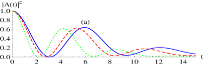
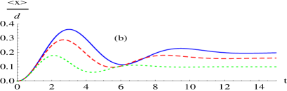
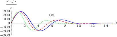
Figure 1: Plots of (a) square of the autocorrelation function, (b) position, and (c) velocity expectation values for $a_{0}=10$. Solid, dashed, and dotted line represent $\eta=0$, $0.5$, and $1$, respectively. Here, $t$ is considered in units of $10^{-3}\hbar d^{3}/(2\alpha)$.

III.3 Transient zitterbewegung in position and velocity

In Fig. 1 we have shown the time variation of the square of the autocorrelation function ($|A(t)|^{2}$), expectation values of position $\langle x(t)\rangle$ and velocity $\langle v_{x}(t)\rangle$ operators for a fixed $a_{0}=10$ and different $\eta=0$, $0.5$, and $1$. The autocorrelation function mainly measures the overlap of the time evolved wave packet with its initial counterpart and is defined as $A(t)=\langle\Psi({\bf r},t)|\Psi({\bf r},0)\rangle=\int d^{2}k\,\Phi^{\dagger}({\bf k},t)\Phi({\bf k},0)$. Now using Eq. (14), it is straightforward to find $A(t)$ in the following form

$$A(t) = \frac{1}{\pi}e^{-a_{0}^{2}}\int d\theta\,dq\,q\,e^{-q^{2}+2a_{0}q\sin\theta}\,e^{i\frac{\hbar q^{2}t}{2m^{\ast}d^{2}}}\cos\Big{(}\frac{\Omega_{q}t}{2}\Big{)}$$

Note that for a finite $\alpha\neq 0$, $\beta\neq 0$, the integrals over $q$ and $\theta$ appearing in Eqs. (16), (19), and (III.3) can not be done exactly and hence numerical treatment has to be implemented to see the explicit time dependence of $|A(t)|^{2}$, $\langle x(t)\rangle$, and $\langle v_{x}(t)\rangle$. From Fig. 1(b) and Fig. 1(c) it is evident that the ZB, appearing in position and velocity, shows transient oscillations. The time scale associated with ZB can not be extracted analytically. However, the transient character of $\langle x(t)\rangle$ and $\langle v_{x}(t)\rangle$ may be explained from the behavior of the autocorrelation function which is shown in Fig. 1(a). $|A(t)|^{2}$ exhibits damped oscillatory character. Fig. 1 clearly shows that the oscillations associated with ZB stop when the autocorrelation function nearly dies out. Now the effect of an enhancement of $\beta$ on ZB is twofold. First, it introduces a phase in the oscillations and second, the amplitude of ZB decreases with the increase of $\beta$ as evident from Fig. 1(b).

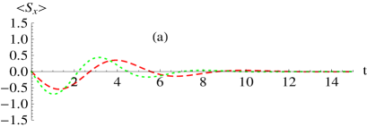
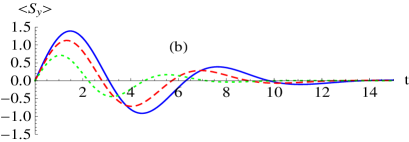
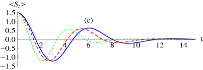
Figure 2: Plots of the expectation values of the spin operators for $a_{0}=10$. Solid, dashed, and dotted line represent $\eta=0$, $0.5$, and $1$, respectively. Here, $t$ is considered in units of $10^{-3}\hbar d^{3}/(2\alpha)$.

IV Spin dynamics and spin-orbit force

Here, we are interested to study the time dependence of the expectation values of the effective spin operator and the spin-orbit force. Due to the existence of SOIs, the spin ${\bf S}=(3/2)\hbar{\bm{\sigma}}$ associated with the HH precesses about an effective magnetic field ${\bf\Omega}$ in accordance with the following equation

$$\frac{d{\bf S}}{dt}={\bf\Omega}\times{\bf S}.$$ (23)

The components of $\bf{\Omega}$ can be obtained as

$$\Omega_{x}=\frac{2}{\hbar^{4}}[\alpha p_{y}(3p_{x}^{2}-p_{y}^{2})-\beta p^{2}p_{x}]$$

and

$$\Omega_{y}=\frac{2}{\hbar^{4}}[\alpha p_{x}(3p_{y}^{2}-p_{x}^{2})-\beta p^{2}p_{y}].$$

The general solution of Eq. (23) is given by

$${\bf S} = (\hat{n}\cdot{\bf S}_{0})\hat{n}+[{\bf S}_{0}-(\hat{n}\cdot{\bf S}_{0})\hat{n}]\cos(\Omega t)$$ (24)

$$+ (\hat{n}\times{\bf S}_{0})\sin(\Omega t),$$

where $\Omega=\sqrt{\Omega_{x}^{2}+\Omega_{y}^{2}}$, ${\bf S}_{0}$ is determined from the initial condition, and the unit vector $\hat{n}$ is defined as $\hat{n}={\bf\Omega}/\Omega$. Without any loss of generality, we choose the initial condition such that $\hat{n}\cdot{\bf S}_{0}=0$ or equivalently, ${\bf S}_{0}=S_{z}\hat{z}$ since $\hat{n}$ lies in the $xy$ plane. So, one can obtain the components of the effective spin operator at a later time $t$ as $S_{x}(t)=(\Omega_{y}/\Omega)S_{z}\sin(\Omega t)$, $S_{y}(t)=-(\Omega_{x}/\Omega)S_{z}\sin(\Omega t)$, and $S_{z}(t)=S_{z}\cos(\Omega t)$. We find the expectation values of the spin components at time $t$ as

$$\left(\begin{array}[]{c}\langle S_{x}(t)\rangle\\ \langle S_{y}(t)\rangle\end{array}\right) = -\frac{3\hbar}{2\pi}e^{-a_{0}^{2}}\int^{2\pi}_{0}d\theta\int_{0}^{\infty}dq\,q\,e^{-q^{2}+2a_{0}q\sin\theta}$$ (27)

$$\times \sin(\Omega_{q}t)\left(\begin{array}[]{c}\cos(3\theta)+\eta\sin\theta\\ \sin(3\theta)-\eta\cos\theta\end{array}\right)$$ (30)

and

$$\langle S_{z}(t)\rangle = -\frac{3\hbar}{2\pi}e^{-a_{0}^{2}}\int^{2\pi}_{0}d\theta\int_{0}^{\infty}dq\,q\,e^{-q^{2}+2a_{0}q\sin\theta}$$ (31)

$$\times \cos(\Omega_{q}t).$$

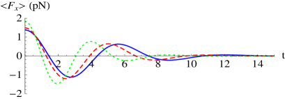
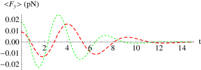
Figure 3: Plots of the expectation values of spin-orbit force operators for $a_{0}=10$. Solid, dashed, and dotted line represent $\eta=0$, $0.5$, and $1$, respectively. Here, $t$ is considered in units of $10^{-3}\hbar d^{3}/(2\alpha)$.

Let us now derive the expression of the spin-orbit force. The spin-orbit force is defined as ${\bf F}=m^{\ast}\ddot{\bf r}$, where $\ddot{\bf r}$ can be evaluated from Heisenberg equation $\ddot{\bf r}=-[[{\bf r},H],H]/\hbar^{2}$. Now, it is straightforward to obtain ${\bf F}$ in the following operator form

$${\bf F} = \frac{2m^{\ast}p^{2}}{\hbar^{7}}\Big{[}(3\alpha^{2}+\beta^{2})p^{2}-8\alpha\beta p_{x}p_{y}\Big{]}({\bf p}\times\hat{z})\sigma_{z}.$$ (32)

Using Eq. (14) we calculate the expectation values for the the components of the spin force operator as

$$\left(\begin{array}[]{c}\langle F_{x}(t)\rangle\\ \langle F_{y}(t)\rangle\end{array}\right) = \frac{2m^{\ast}\alpha^{2}}{\pi\hbar^{2}d^{5}}e^{-a_{0}^{2}}\int^{2\pi}_{0}d\theta\int_{0}^{\infty}dq\,e^{-q^{2}+2a_{0}q\sin\theta}$$ (35)

$$\times q^{6}\cos(\Omega_{q}t)g(\theta)\left(\begin{array}[]{c}\sin\theta\\ -\cos\theta\end{array}\right).$$ (38)

In Fig. 2 and Fig. 3, we have shown the time dependence of the expectation values of spin and spin-orbit force operators. From Fig. 2 it is evident that $\langle S_{x}(t)\rangle$ vanishes in the absence of the Dresselhaus SOI. When $\beta=0$ the angular integrations in Eqs. (27) and (31) can be done exactly which gives a vanishing result for $\langle S_{x}\rangle$. The other components of the spin operator i.e. $\langle S_{y}(t)\rangle$ and $\langle S_{z}(t)\rangle$ can be found in the following forms

$$\langle S_{y}(t)\rangle=3\hbar e^{-a_{0}^{2}}\int_{0}^{\infty}dq\,qe^{-q^{2}}I_{3}(2a_{0}q)\sin\Big{(}\frac{2\alpha}{\hbar d^{3}}q^{3}t\Big{)}$$ (39)

and

$$\langle S_{z}(t)\rangle=3\hbar e^{-a_{0}^{2}}\int_{0}^{\infty}dq\,qe^{-q^{2}}I_{0}(2a_{0}q)\cos\Big{(}\frac{2\alpha}{\hbar d^{3}}q^{3}t\Big{)},$$ (40)

where $I_{n}(z)$ is the modified Bessel function of first kind. Eqs. (39) and (40) indicate that the spin precesses in the $yz$ plane. For $\beta=0$, one can find that $\langle F_{y}(t)\rangle=0$. In this case, $\langle F_{x}(t)\rangle$ takes the following form

$$\langle F_{x}(t)\rangle=F_{0}e^{-a_{0}^{2}}\int_{0}^{\infty}dq\,q^{6}e^{-q^{2}}I_{1}(2a_{0}q)\cos\Big{(}\frac{2\alpha}{\hbar d^{3}}q^{3}t\Big{)},$$ (41)

where $F_{0}=12m^{\ast}\alpha^{2}/(\hbar^{2}d^{5})$. Analyzing Eqs. (39)-(41), one can conclude that the spin precession in the $yz$ plane essentially generates a transverse spin-orbit force along $x$ direction. This fact is depicted in Fig. 3.

The scenario changes significantly in the presence of a finite $\beta$. In this case the angular integrations in Eqs. (27)-(31) and Eq. (35) can not be done exactly. A numerical calculation shows that $\langle S_{x}(t)\rangle$ survives for $\beta\neq 0$ but its magnitude is small compared to that of $\langle S_{y}(t)\rangle$ and $\langle S_{z}(t)\rangle$. Thus the spin starts to precess in the entire space as one switches on $\beta$. As a result, a finite $y$ component of the spin-orbit force is generated. But the amplitude of $\langle F_{y}\rangle$ is negligibly small in comparison to that of $\langle F_{x}\rangle$ as evident from Fig. 3. So, one can safely consider that the spin-orbit force acts along the $x$ direction provided the initial wave packet is injected along the $y$ direction. In recent pastzb2d1 , the origin of ZB was explained in the light of the spin-orbit force and it was argued that ZB occurs in a direction along which the spin-orbit force acts on the wave packet. By observing Eqs. (16), (19), and (41), we conclude that our results are consistent with that prediction.

V Persistent Zitterbewegung and Possible detection

The ZB, manifested in the expectation values of the physical observables undergo transient behavior. However, the persistent behavior of ZB can be obtained in the limit $a_{0}\gg 1$ i. e. the initial wave packet is sharply peaked in the momentum space. For $\beta=0$, one can obtain the following approximate expressions for the expectation values: $\langle x\rangle\simeq(3/2k_{0})[1-\cos(\omega_{0}t)]$, $\langle v_{x}\rangle\simeq(3\alpha k_{0}^{2}/\hbar)\sin(\omega_{0}t)$, $\langle S_{y}\rangle\simeq(3\hbar/2)\sin(\omega_{0}t)$, $\langle S_{z}\rangle\simeq(3\hbar/2)\cos(\omega_{0}t)$, and $\langle F_{x}\rangle\simeq f_{0}\cos(\omega_{0}t)$ where $\omega_{0}=2\alpha k_{0}^{3}/\hbar$ and $f_{0}=6m^{\ast}\alpha^{2}k_{0}^{5}/\hbar^{2}$. Due to the presence of SOI, an effective Lorentz-like magnetic fieldpal can be obtained in the following form ${\bf B}_{\rm s}=2m^{\ast 2}\alpha^{2}p^{4}g(\theta)\sigma_{z}\hat{z}/(e\hbar^{7})$. In the $a_{0}\gg 1$ limit and when $\beta=0$ we obtain $\langle B_{\rm s}\rangle\simeq B_{0}\cos(\omega_{0}t)$ where $B_{0}=6m^{\ast 2}\alpha^{2}k_{0}^{4}/(e\hbar^{3})$. Interestingly, we find $\langle F_{x}\rangle/\langle B_{\rm s}\rangle=e\hbar k_{0}/m^{\ast}$ i.e. $F_{x}$ plays a role of the Lorentz force in the $a_{0}\gg 1$ limit. Now, the time dependent magnetic field $B_{s}$ would generate an electric voltage of the following form $V=V_{0}\sin(\omega_{0}t)$ where $V_{0}=\omega_{0}AB_{0}$ with $A$ as the area of the sample. For typical material parameters a GaAs quantum well i.e. $m^{\ast}=0.45m_{e}$, $\alpha=10^{-28}$ eVm³, $A=10^{4}$ nm², and $k_{0}=10^{8}$ m^-1 we obtain $\omega_{0}\simeq 3\times 10^{11}$ rad/s, $B_{0}\simeq 0.14$ T, and $V_{0}\simeq 4.4\times 10^{-4}$ V. In principle, one can measure $V_{0}$ to confirm the signature of ZB experimentally. As introduced recentlyzb2d5 this kind of electric voltage associated with ZB can be also obtained in the case of a 2DEG with time dependent linear Rashba SOI.

VI Summary

In summary, we have investigated the $zitterbewegung$ of a wave packet in a 2DHG in the presence of both Rashba and Dresselhaus SOIs. The $zitterbewegung$ manifested in position, velocity, and spin appear as transient oscillations. For equal strength of Rashba and Dresselhaus SOIs we find $zitterbewegung$ does not vanish, a direct contradiction to the electronic case. This non-vanishing of $zitterbewegung$ has been interpreted as a consequence of the Berry phase. The pseudo-spin associated with the heavy hole precesses about a SOI induced effective magnetic field. As a consequence of this spin precession, a transverse component of the spin-orbit force appears which in turn induces $zitterbewegung$ in position and velocity. The transverse spin-orbit force also generates an electric voltage. We have concluded that an indirect signature of $zitterbewegung$ can be unveiled by measuring this voltage.

References

• (1) E. Schrödinger, Sitzungsber. Preuss. Akad. Wiss., Phys. Math. Kl. 24, 418 (1930); A. O. Barut and A. J. Bracken, Phys. Rev. D 23, 2454 (1981).
• (2) W. Zawadzki and T. M. Rusin, J. Phys.: Condens. Matter 23, 143201 (2011).
• (3) W. Zawadzki, Phys. Rev. B 72, 085217 (2005).
• (4) J. Schliemann, D. Loss, and R. M. Westervelt, Phys. Rev. Lett. 94, 206801 (2005).
• (5) S. Q. Shen, Phys. Rev. Lett. 95, 187203 (2005).
• (6) J. Schliemann, D. Loss, and R. M. Westervelt, Phys. Rev. B 73, 085323 (2006).
• (7) V. Ya. Demikhovskii, G. M. Maksimova, and E. V. Frolova, Phys. Rev. B 78, 115401 (2008).
• (8) T. Biswas and T. K. Ghosh, J. Phys.: Condens. Matter 24, 185304 (2012).
• (9) T. Biswas and T. K. Ghosh, J. Appl. Phys. 115, 213701 (2014).
• (10) C. S. Ho, M. B. A. Jalil, and S. G. Tan, EPL, 108, 27012 (2014).
• (11) T. M. Rusin and W. Zawadzki, Phys. Rev. B 76, 195439 (2007).
• (12) T. M. Rusin and W. Zawadzki, Phys. Rev. B 78, 125419 (2008).
• (13) G. M. Maksimova, V. Ya. Demikhovskii, and E. V. Frolova, Phys. Rev. B 78, 235321 (2008).
• (14) J. Schliemann, New J. Phys. 10, 043024 (2008).
• (15) Q. Wang, R. Shen, L. Sheng, B. G. Wang, and D. Y. Xing, Phys. Rev. A 89, 022121 (2014).
• (16) W. Zawadzki, Phys. Rev. B 74, 205439 (2006).
• (17) L. K. Shi, S.C. Zhang, and K. Chang, Phys. Rev. B 87, 161115 (R) (2013).
• (18) J. Cserti and G. David, Phys. Rev. B 74, 172305 (2006).
• (19) X. Zhang and Z. Liu, Phys. Rev. Lett. 101, 264303 (2008).
• (20) X. Zhang, Phys. Rev. Lett. 100, 113903 (2008).
• (21) F. Dreisow, M. Heinrich, R. Keil, A. Tunnermann, S. Nolte, S. Longhi, and A. Szameit, Phys. Rev. Lett. 105, 143902 (2010).
• (22) J. Y. Vaishnav and C. W. Clark, Phys. Rev. Lett. 100, 153002 (2008).
• (23) Y. C. Zhang, S. W. Song, C. F. Liu, and W. M. Liu, Phys. Rev. A 87, 023612 (2013).
• (24) L. J. LeBlanc, M. C. Beeler, K. Jimenez-Garcia, A. R. Perry, S. Sugawa, R. A. Williams, and I. B. Spielman, New J. Phys. 15, 073011 (2013).
• (25) C. Qu, C. Hamner, M. Gong, C. Zhang, and P. Engels, Phys. Rev. A 88, 021604(R) (2013).
• (26) A. Singh, T. Biswas, T. K. Ghosh, and A. Agarwal, Eur. Phys. J. B 87, 275 (2014).
• (27) A. Singh, T. Biswas, T. K. Ghosh, and A. Agarwal, Ann. Phys. 354, 274 (2015).
• (28) R. Winkler, Spin-Orbit Coupling effets in Two-Dimensional Electron and Hole Systems (Springer, Berlin, 2003).
• (29) J. Nitta, F. E. Meijer, and H. Takayanagi, Appl. Phys. Lett. 75, 695 (1999).
• (30) D. Awschalom, N. Samarth, and D. Loss, Semiconductor Spintronics and Quantum Computation (Springer-Verlag, Berlin, 2002).
• (31) T. Koga, J. Nitta, H. Takayanagi, and S. Datta, Phys. Rev. Lett. 88, 126601 (2002).
• (32) T. Koga, J. Nitta, and M. van Veenhuizen, Phys. Rev. B 70, 161302 (2004).
• (33) T. Koga, Y. Sekine, and J. Nitta, Phys. Rev. B 74, 041302 (2006).
• (34) B. Das, S. Datta, and R. Reifenberger, Phys. Rev. B 41, 8278 (1990).
• (35) J. E. Hirsch, Phys. Rev. Lett. 83, 1834 (1999).
• (36) S. Murakami, N. Nagaosa, and S. C. Zhang, Science 301, 1348 (2003).
• (37) Y. K. Kato, R. C. Myers, A. C. Gossard, and D. D. Awschalom, Science 306, 1910 (2004).
• (38) C. L. Kane and E. J. Mele, Phys. Rev. Lett. 95, 146802 (2005).
• (39) B. A. Bernevig and S. C. Zhang, Phys. Rev. Lett. 96, 106802 (2006).
• (40) B. A. Bernevig, J. Orenstein, and S. C. Zhang, Phys. Rev. Lett. 97, 236601 (2006).
• (41) J. D. Koralek, C. P. Weber, J. Orenstein, B. A. Bernevig, S. C. Zhang, S. Mack, and D. D. Awschalom, Nature 458, 610 (2009).
• (42) Y. A. Bychkov and E. I. Rashba, J. Phys. C 17, 6039 (1984).
• (43) E. I. Rashba and E. Ya. Sherman, Phys. Lett. A 129, 175 (1988).
• (44) G. Dresselhaus, Phys. Rev. 100, 580 (1955).
• (45) J. Schliemann and D. Loss, Phys. Rev. B 71, 085308 (2005).
• (46) T. Ma and Q. Liu, Phys. Rev. B 73, 245315 (2006).
• (47) O. Bleibaum and S. Wachsmuth, Phys. Rev. B 74, 195330 (2006).
• (48) H. Nakamura, T. Koga, and T. Kimura, Phys. Rev. Lett. 108, 206601 (2012).
• (49) R. Moriya, K. Sawano, Y. Hoshi, S. Masubuchi, Y. Shiraki, A. Wild, C. Neumann, G. Abstreiter, D. Bougeard, T. Koga, and T. Machida, Phys. Rev. Lett. 113, 086601 (2014).
• (50) J. M. Luttinger, Phys. Rev. 102, 1030 (1956).
• (51) D. V. Bulaev and D. Loss, Phys. Rev. Lett. 95, 076805 (2005).
• (52) A. Wong and F. Mireles, Phys. Rev. B 81, 085304 (2010).
• (53) S. Q. Shen, Phys. Rev. B 70, 081311 (2004).
• (54) B. Paul and T. K. Ghosh, Phys. Lett. A 379, 728 (2014).