Nonparametric Bayesian Modeling for
Automated Database Schema Matching

Abstract

The problem of merging databases arises in many government and commercial applications. Schema matching, a common first step, identifies equivalent fields between databases. We introduce a schema matching framework that builds nonparametric Bayesian models for each field and compares them by computing the probability that a single model could have generated both fields. Our experiments show that our method is more accurate and faster than the existing instance-based matching algorithms in part because of the use of nonparametric Bayesian models.

1 Background and Motivation.

The trend health care, finance, and government sectors toward data sharing has increased the need for data integration. Furthermore, organizations are mandated to integrate their data, whether due to a corporate merger, legislated duties, international military efforts, or disaster management. A strong economic incentive exists for data integration resulting from its benefits for anomaly detection, data quality processing, fraud detection, and streamlining processing.

The data integration problem includes both schema matching and coreference as subproblems. Schema matching is the problem of identifying fields that refer to the same concepts. Coreferencing is the problem of identifying records that refer to the same underlying entity. The difficulty of automatically attaining high quality matches has motivated research to learn the schema matching using a small number of coreferents [18, 6, 5], to learn coreferents given a matched schema [2], and to learn both schema and coreferents simultaneously [22]. However, there is a need for an out-of-the-box schema matching solution that is independent of coreferencing. This paper contributes to that goal.

Methods for automating schema matching have been explored in the scientific literature [3] and have been included as part of business analytics tools (by, e.g., IBM, SAS, Oracle, and Microsoft). The majority of this work has focused on using available metadata such as field names, on providing user interfaces for manual field linking, and on developing effective matchers as ensembles of individual matchers. We review the related work in Section 1.1. Despite all of this previous work, practical exercises of data integration continue to be largely manual processes.

The primary contributions of this paper are

• a set of three nonparametric Bayesian model classes for use within a new probability-based schema matching framework (Section 2),

• evidence that these model classes outperform existing instance-based matching scores (described in Section 1.2) in both accuracy and speed (Section 3.3), and

• evidence that the improved performance is due at least in part to the use of nonparametric Bayesian models (Section 4).

1.1 Related Work.

A majority of previous work has been devoted to using metadata for matching fields [3]. These methods include exact and inexact [5] matching of field names, synonym-based matching [10], and other language-based analyses [15]. These methods assume a coherence between named fields and are likely to perform poorly if the same data is called, say, Customer Name in one data set and Guest ID in another.

Many existing machine learning methods attempt to learn how to match names or other metadata using dictionaries or natural language processing methods. Those methods incur the additional burden of obtaining a good good training set or solving the associated transfer learning problem. Either concern weakens the generalizability of any proposed system, as the solutions to these problems may be domain specific.

It should be noted that matchers are typically used in combination, as this practice has been shown to be effective [8, 4]. However, to help clarify the impact of our contributions, we focus on each instance-based matcher separately.

Our approach is fully instance-based and ignores any metadata that may be available. Some previous work has been instance-based. Instance-based methods use each field to produce a summary and then compare the summaries. These summaries tend to be the set or multiset of values. We compare our framework against the best instance-based methods in the literature.

More recently, especially as researchers have shifted their focus from databases to ontologies, additional emphasis has been placed on exploiting the relationships among fields (also called concepts in the ontology context), such as is-a and has-a relationships. Because these methods are applied to expert-developed ontologies (e.g., different anatomy ontologies) there are generally only a few available instances for each field. Methods exist to leverage known matched instances for schema matching [9]. Such matched pairs provide a significant advantage in finding schema matches. In many applications, including typical cross-organizational data integration efforts, the existence of common referents cannot be assumed. Furthermore, even if such common referents exist, finding them is itself a highly challenging research problem. Our method does not depend on having coreferents.

1.2 Baseline Methods.

Instance-based schema matching is generally pursued by defining similarity or distance metrics between two fields, and then using these scores to determine the matching decisions. There are several field matching scores that have been studied in the literature. We compare our method to five prominant and representative similarity scores. Two scores are based on set intersections and three scores use the full multiset of counts. The Jaccard Coefficient and the Pointwise Mutual Information are described in [11, 21]. So-called corrected versions are also described, but we will not discuss them here since they consistently underperformed the uncorrected versions in all of our experiments. Kang and Naughton (2003) introduce information-theoretic measures based on mutual information and entropy. Jaiswal et al. (2010) introduce the Euclidean distance on the sorted normalized value counts. Their use of the distance on the sorted counts is meant to support detecting value transformations, which we do not consider. The natural alternative is to use the Euclidean distance on the unsorted normalized value counts, which we also include although they did not explicitly define or use it.

To define the baseline methods, we use the following notation for a fixed pair of match candidates. Let $C$ and $D$ be sets of observed values from the two fields, $N$ be the total number of observations, including repititions, $p_{i}$ and $q_{i}$ be the proportion of observations that were equal to the $i$-th distinct value, and $p^{\prime}$ and $q^{\prime}$ be $p$ and $q$, respectively, but each in decreasing order. The names for the following statistics are chosen consistently with the literature.

Jaccard Coefficient $$\frac{|C\cap D|}{|C\cup D|}$$

Pointwise MI $$\log_{2}\frac{|C\cap D|\times N}{|C||D|}$$

Entropy Difference $$\left|\sum_{i}p_{i}\log p_{i}-\sum_{i}q_{i}\log q_{i}\right|$$

Unsorted Euclidean $$\sum_{i}(p_{i}-q_{i})^{2}$$

Sorted Euclidean $$\sum_{i}(p^{\prime}_{i}-q^{\prime}_{i})^{2}$$

The first two scores give larger values for more likely matches, whereas the other scores (the last three) give smaller values for more likely matches. Two additional similarity scores, Jensen-Shannon and log likelihood, are considered in the literature, but we do not include them here since they require the set of observed values to be the same for both fields, which is almost never the case.

The references apply the metrics within more complex matching schemes using ensemble scores [19], limits on the number of matches per field [16], and collective optimization [17]. For clarity, we focus on the more straightforward, though harder, problem of deciding whether two sets of instances should be matched or not, without regard to the other available information and restrictions.

The variety of set-based and multiset-based similarity functions studied have two main shortcomings. First, they are very coarse in the sense that a lot of information regarding similarities between values is discarded. Second, they tend to be computationally very expensive. In many cases, these methods require comparing every value in one field to every value in the other, which is work on the order of the number of distinct values for each pair.

Non-multiset-based methods have been explored in the literature. For example, Jaiswal et al. model continuous variables by Gaussian mixtures. Other research has pursued value classification [13] and clustering approaches [14, 1]. We do not compare directly to these alternative methods, primarily because they are computationally prohibitive for large data sets.

2 Methods and Technical Solutions.

We explore the hypothesis that using probabilistic models that meet certain simplicity constraints enable both greater accuracy and greater computational efficiency. We view field values as being generated according to probabilistic models, which allows for explicit computation of the probability of a match given the observed data.

The probabilistic field matching framework uses a collection of model classes to (1) train models based on string instances observed in each field, and (2) compare models by computing the relative likelihood that both fields were generated from the same models.

The process of matching fields is then as follows. First, initial models are created for each field for each model class and then updated efficiently with the data from that field by computing the sufficient statistics that determine the parameters (see next section for model-specific details). Second, the probability of a match for each pair is computed.

We pose the field match problem as a probability computation. For any pair of fields, we assume two mutually exclusive and exhaustive possibilities, either (1) there was one model generating both fields, or (2) the fields were generated by independent models. We denote the former as $S$ and the latter as $\neg S$. By Bayes’ rule, the probability of a match for field data $X$ and $Y$ is then $\mathrm{P}(S\mid X+Y)=$

$$\frac{\mathrm{P}(X+Y\mid S)\mathrm{P}(S)}{\mathrm{P}(X+Y\mid S)\mathrm{P}(S)+\mathrm{P}(X+Y\mid\neg S)\mathrm{P}(\neg S)},$$ (1)

with $\mathrm{P}(X+Y\mid\neg S)=\mathrm{P}(X)\mathrm{P}(Y)$, since it uses independent models for $X$ and $Y$. This computation is done for each model class separately. Generally, the match scores will form the basis for follow-on processing for data integration or other related purposes.

We created and implemented three probabilistic model classes for string generation satisfying the design constraints. Each model class uses the Chinese Restaurant Process (CRP) in modeling the collection of all possible strings. The CRP may be viewed as a principled generalization of a Dirichlet distribution to infinite dimensions that maintains exchangeability and has no zero probabilities (provided that the base distribution has none). The use of the CRP, while not new in the literature, is somewhat unusual due to the fact that we are working with a probability mass function rather than a probability density function.

The possible values for a field will only rarely be known in advance. Consequently, typical methods for modeling categorical data, such as multinomial distributions, will usually not apply. Instead, Dirichlet processes are appropriate. A Dirichlet process is a stochastic process that generates a Dirichlet distribution. Loosely speaking, the Dirichlet process provides a way to select a finite number of categories and to build a multinomial for it, while still allowing for the possibility of new events. Although a full technical description of Dirichlet processes is beyond the scope of this paper, only an understanding of the probability scoring described in (2) will be needed. A thorough survey is available from [20].

One useful metaphor for the Dirichlet process is the Chinese Restaurant Process (CRP). The CRP models a series of arrivals at a restaurant that has a countably infinite number of tables with unlimited seating. A new customer either chooses a table with probability proportional to the number of customers already seated at the table or else picks a new table with probability proportional to the concentration parameter $\alpha$. The first customer necessarily picks a new table. Every time a new table is selected, a label is generated according to a specified base distribution. In the typical treatment, the base distribution is assumed to be non-atomic, so that the probability of a subsequent new table generating a repeated label is zero. In the Atomic CRP, this assumption is waived. The fundamental theory remains the same. Without loss of generality, a customer at a new table that chooses a repeated label is moved to the table already having that label.

The probability of getting $m_{i}$ instances of value $x_{i}$ where the $x_{i}$ are generated according to a base distribution $H$ in a CRP with parameter $\alpha$ is given by

$$\frac{\Gamma(\alpha)}{\Gamma(\alpha+\sum_{i}m_{i})}\prod_{i}\frac{\Gamma(\alpha H(x_{i})+m_{i})}{\Gamma(\alpha H(x_{i}))},$$ (2)

where $\Gamma$ is the standard Gamma function. By comparison, the non-atomic CRP is obtainable from (2) by replacing $H(x_{i})$ with 1. Of course, the two versions of the CRP model slightly different data since only the ACRP accounts for the labels.

2.1 Discrete Model.

The discrete model class is the simplest of the three model classes. The table labels from the Atomic Chinese Restaurant Process are the set of distinct values in the field. As a base distribution ($H$ in (2)), we choose the following string generation process. First, select a string length according to a Poisson distribution with fixed $\lambda$. Next, generate that many uniformly chosen characters from the alphabet. A discrete model must track the entire multiset of observations.

To compute the probability of the data, we use the standard Bayesian paradigm. For $M$ the model class and strings $x_{1},x_{2},\dots,x_{n}$,

$$\mathrm{P}(x_{1}, x_{2},\dots,x_{n}\mid M)=$$

$$\prod_{i=1}^{n}\mathrm{P}(x_{i}\mid M,x_{1},x_{2},\dots,x_{i-1})$$

where each term uses the parameters computed from the previous data to calculate the probability of the next observation. The joint probability is exchangeable; it does not matter in what order the data are observed. Moreover, the joint probability can be computed directly and quickly from the parameters in terms of the Gamma function, as per (2).

2.2 Positional Model.

We define a positional probability model that generates strings in two steps. First, a length $\ell$ is sampled from an Atomic Chinese Restaurant Process with a Poisson base distribution. Second, $\ell$ characters are sampled from the first $\ell$ character distributions, which are modeled with separate uniform Dirichlet distributions on a fixed known alphabet $A$. The model parameters for this model are computed by counting the number of strings of each length and the number of times each character is observed at each position. Let $n_{\ell}$ be the number of strings of length $\ell$. For $j=1,2,\dots$ and for $a\in A$ a character in the fixed alphabet, let $c_{j,a}$ be the number of times character $a$ was observed in position $j$. The probability of the $i$-th string $x_{i,1}x_{i,2}\dots x_{i,\ell_{i}}$ for $\ell_{i}$ its length is the probability of the length times the probabilities of the characters.

$$\mathrm{P}(x_{i,1} x_{i,2}\dots x_{i,\ell_{i}}\mid n,c,\alpha,\lambda,\beta)=$$ (3)

$$\frac{n_{\ell_{i}}+\alpha\text{Pois}_{\lambda}(\ell_{i})}{n+\alpha}\prod_{j=1}^{\ell_{i}}\frac{c_{j,x_{j}}+\beta}{n_{\geq j}+|A|\beta}$$ (4)

where $\alpha$ is the CRP strength parameter for the length, $\lambda$ is the parameter for the CRP’s Poisson base distribution, $\beta$ is the Dirichlet prior for all character multinomials, $|A|$ the fixed alphabet size, and $n_{\geq j}$ is for the number of strings observed with length at least $j$. Also, an empty product is 1 by convention. Equation (3) is useful for computing the probability of a single string and could be used to compute the joint probability of the data, but a simpler product using the Gamma function is possible.

$$\mathrm{P}(x_{1},x_{2}, \dots,x_{n}\mid M)=\frac{\Gamma(n_{\ell}+\alpha\text{Pois}_{\lambda}(\ell))\Gamma(\alpha)}{\Gamma(\alpha\text{Pois}_{\lambda}(\ell))\Gamma(n+\alpha)}$$

$$\prod_{j=1}^{\max\ell} \prod_{a\in A}\frac{\Gamma(c_{j,a}+\beta)}{\Gamma(\beta)}\frac{\Gamma(|A|\beta)}{\Gamma(n_{\geq j}+|A|\beta)}$$ (5)

where $M$ denotes the model class.

The positional model must track the number of times each character was observed in each position as well as the number of strings of each length. The parameters for the combined data from two columns are the sum of the parameters learned from each column. The joint probability is computable in time proportional to the number of parameters, rather than in time proportional to the amount of data, a fact that is especially important when computing the probability that two fields were generated from the same model. That is, $c^{(X+Y)}_{j,a}=c^{(X)}_{j,a}+c^{(Y)}_{j,a}$ for all $j$ and $a$.

2.3 Apositional Model.

The apositional model is a simplification of the positional model. In generating strings, it chooses the length in the same way. However, the characters are produced with probabilities that are independent of the position. The probability of data given the model can be computed using the same formulas, but in place of $c_{i,a}$ we use

$$c^{\prime}_{a}=\sum_{i}c_{i,a}.$$

That is, the counts are combined across positions. Alternatively, it can be viewed as imposing a parameter equality across the positions. To combine two models’ parameters $c$ and $n$, we again simply add them.

3 Empirical Evaluation.

We tested our nonparametric Bayesian schema matching approach with a number of experiments. The experimental procedures followed are described in Subsection 3.1. The data sets are described in Subsection 3.2.

3.1 Experimental Design.

To measure the accuracy of the schema matching, we performed a subsample self-match. First, the data sets are cleaned. Strings are normalized to a 64 character alphabet by capitalizing all letters and replacing any character that is not a digit or a punctuation mark (in particular, period, comma, colon, semi-colon, slash, backslash, quote, apostrophe, back tick, bracket, parenthesis, plus, minus, exclamation mark, question mark, dollar sign, percent, ampersand, asterisk, underscore) with a placeholder symbol. Fields in which 99% of the values were the same were removed; this included removing empty fields since all their values were empty strings. Second, we create two subsample data sets with the first and last $n$ records. Third, we take ground truth to be that the $i$-th field of one sample only matches the $i$-th field of the other sample. This is not a perfect assumption in the sense that multiple fields can represent the same type of data (e.g., dates). However, since subsample self-matching enables a consistent comparison between methods and across data sets with reliable ground truth, subsample matching has become standard [12]. Fourth, we run the baseline schema matching methods and our probabilistic field modeling approach to match fields between the two subsamples. Every pair of one field from the first subsample and one field from the second is then an example that is scored and compared to ground truth. Given $d$ fields, we obtain $d^{2}$ examples, of which $d$ are matches and $d^{2}-d$ are non-matches. We compute standard machine learning measures of success, including the ROC curve and the area under the ROC curve.

In the literature it is common to downselect the number of features used in pairwise match computations to ten to thirty. Furthermore, they often include constraints on the number of matches allowed for any given field, such as limiting every field in one data set to at most one match in the other data set [7]. These sorts of assumptions, while often reasonable, will not be valid in general. Consequently, we preferred to test our method in the more realistic and more difficult case where no constraints are known.

All models were chosen using the same priors and base distributions. The parameter $\alpha$ for the Chinese Restaurant Process for the string length was 3.0. The mean string length $\lambda$ was 4.0. The prior $\beta$ for the character distributions was 3.0.

3.2 Data.

We tested our schema matching algorithm on four different data sets: Census, Loans, Mix Market, and NPPES. Table 1 provides the number of records, the original number of fields, and the number remaining after removing empty and nearly constant fields.

Table 1: Data Set Sizes

		Orig.	Filtered
Data Set	Records	Fields	Fields
Census	581746	118	101
Loans	147638	101	100
Mix Market	14736	83	81
NPPES	1308299	329	101

The Census data comes from the 1990 Census, and is provided by The United States Census Bureau provides the 1990 Public Use Micro Sample 5% data from California. The fields are fixed-width numeric encodings according to a data dictionary. We did not replace the codes with their dictionary values.

The Loans data contains complete loan information, such as loan status and payment information. The data come from Lending Club, an online financial community that matches individual borrowers with individual lenders and has loaned over $2.5 billion dollars to date. The fields include durations, amounts, percentages, and dates.

The Mix Market data come from Microfinance Information Exchange, Inc., a non-profit organization that manages and provides information about financial institutions engaged in microlending, the practice of making high-impact small-capital loans to disadvantaged borrowers. We used their freely available Basic MIX MFI Data Set. In contrast to the Census data, the Mix Market data presents a wide variety of field types. For example, it includes and ID number, an organization name, currency type and amounts (separately), years, dates, and percentages.

The NPPES data is a large data set managed by Center for Medicare and Medicaid Studies containing public information about registered Medicare service providers. NPPES has by far the largest number of records of our three data sets, which allows us to test our algorithms on especially large data sets. The data contained are diverse, although most of it is comprised of contact information, such as name, phone number, and address fields. Of special interest within the health care domain is the problem of handling the wide diversity of provider IDs that appear in various fields, especially the 73 different “Other Provider Information” fields. These fields are used to collectively capture a list of values, which challenges the accuracy of any automated schema matching solution.

3.3 Results.

Fig. 1 shows that the best classifier on the NPPES data set with samples of size 50,000 is the apositional probability model. The best multiset-based model is the unsorted Euclidean score. The set-based scores performed the worst, but the better one is the Jaccard coefficient. This pattern, in which the probabilistic models perform the best and the set-based methods the worst was consistent across all experiments.

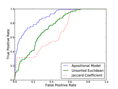
Figure 1: The ROC curve for the apositional field model (the best probabilistic model in this experiment) is superior to both the set-based and multiset-based schema matching approaches for most false positive rates. This comparison is for subsamples of size 50,000 within the NPPES data set.

In many cases the apositional model was the best of the probabilistic models, followed by the positional and discrete models. One exception was in the Census data with samples of size 500 where the discrete model was the best, and the apositional was the worst. Table 2 summarizes the AUC statistics for the probabilistic models across the four data sets with samples of size 5000. In every case, the best model is a nonparametric Bayesian models.

The Table also shows a clear performance gap between set-based and multiset-based methods. The Sorted Euclidean and Unsorted Euclidean scores are consistently better than Entropy Difference or the set-based methods. This observation replicates the findings in [12].

Table 2: AUC for Subsamples of Size 5000.

	Data Set
Model	Census	Loans	Mix	NPPES
Apositional	0.88	0.89	1.00	0.88
Positional	0.87	0.85	0.99	0.87
Discrete	0.91	0.87	0.87	0.79
Sorted Eucl.	0.86	0.68	0.98	0.74
Unsorted Eucl.	0.86	0.71	0.98	0.74
Entropy Diff.	0.82	0.69	0.93	0.70
Jaccard Coef.	0.76	0.57	0.65	0.67
PMI	0.67	0.61	0.60	0.60

The apositional and positional probabilistic models, in addition to often being the best performing, were also significantly faster. One reasonable way to judge the speed of each method is to count the number of parameters it uses. The model training and the field comparison both require work on the order of the number of parameters. This is true also for set-based and multiset-based methods if we take their parameters to be the set and the multiset, resp. Both of these as well as the discrete model have as many parameters as there are distinct values in the field. Table 3 lists the average number of parameters across all fields for NPPES and for each model. It shows that the apositional and positional models computationally scale far better.

Table 3: Average Number of Model Parameters

	Subsample Size
Model	500	5000	50000
Apositional	45	62	77
Positional	214	411	667
All Others	169	1338	10641

4 Significance and Impact.

In this section, we show that using more data helps, but only marginally, especially in comparison to the difference in performance between methods. We then show that the training for the positional and apositional models allow for inference of character-level value patterns. Finally, we show by experiments that the success of our approach is attributable (at least in part) to the properties of nonparametric Bayesian models.

4.1 Sensitivity to Data Size.

We conducted experiments to examine the sensitivity of the determined AUC to changing data size. Table 4 shows that the AUC for the apositional and positional models does not appreciably change with an increase in data size. Also, the difference in performance between models is significantly larger than the gains in performance from a 100-fold increase in data size. The performance difference in the apositional and positional models is especially surprising when considering that they use far fewer paramters (see Table 3).

Table 4: AUC for NPPES with Varying Subsample Sizes.

	Subsample Size
Model	500	5000	50000
Apositional	0.89	0.88	0.89
Positional	0.87	0.87	0.87
Discrete	0.78	0.79	0.83
Sorted Eucl.	0.74	0.74	0.75
Unsorted Eucl.	0.73	0.74	0.75
Entropy Diff.	0.69	0.70	0.72
Jaccard Coef.	0.64	0.67	0.68
PMI	0.59	0.60	0.61

4.2 Pattern Inference.

The positional and apositional models extrapolate based on character-level similarities between values, such as learning formats and other patterns, without having to make a new model for each pattern. In contrast, set and multiset methods cannot. For example, the positional model has learned the structure of date fields in the Loans data set. In particular, the seventh position is a hyphen for correctly coded values. Similarly, the positional model also learned that the first character of the NPI Code field is always the digit 1. Additionally, the apositional model learns that the majority of characters in a ZIP Code field are digits. The fact that it has non-digits suggests a data entry error. Using positional and apositional models allows for the construction of system data quality checks.

4.3 Effect of Bayesian Computations and CRP.

The approach outlined in this paper is focused on a probabilistic framework and the models used within that framework. We have stressed that the models follow the Bayesian paradigm in which the probability of the data is computed, at least theoretically, one observed value at a time. This approach motivated the use of the Chinese Restaurant Process since it follows the paradigm while also allowing for arbitrarily many different values, even if they are not known in advance.

One commonly used approach that contrasts with the Bayesian paradigm is the Maximum Likelihood Estimation (MLE) paradigm, wherein the data are scored according the model that maximizes their likelihood. In using the probabilistic framework, we could have adopted a parametric and non-Bayesian approach where the parameters for the models are learned from the data. In this subsection, we consider three MLE versions of the three probabilistic models we used. These approaches compute the same parameters, but compute the probability of the data by having the probability of an event $x$ as the proportion of previous observations that were $x$. For the apositional and positional models, we also compute the average length of the strings and use that as the mean for the Poisson that generates the string lengths. The character probabilities are set according to the proportion of observations.

By comparing the MLE versions and the Bayesian versions of the probabilistic models, we were able to show that the Bayesian versions generally perform better. Fig. 2 compares these models on the NPPES data set with subsamples of size 50,000; these curves represent the most competitive MLE results obtained. We conclude that the nonparametric Bayesian versions of the probabilistic models attain better performance than the MLE versions.

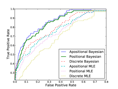
Figure 2: The ROC curve for the nonparametric Bayesian models show better field matching than the Maximum Likelihood Estimation approaches for subsamples of size 50,000 within the NPPES data set.

We explain this difference by considering (1) the MLE training process, (2) Bayes’ rule with the MLE models, and (3) the usefulness of the Chinese Restaurant Process. The MLE training process uses the data both to build the model and compute its probability. Since we are using the probability as an important component in our classification, this approach could lead to overtraining. Also, the probability of two fields coming from the same model (i.e., $\mathrm{P}(S)$) will always be lower than the probability of two fields coming from different models in the MLE paradigm. This is not true for the Bayesian paradigm, and suggests that the MLE paradigm is not correctly addressing the similarity question. Finally, the Chinese Restaurant Process was not part of the MLE models. Consequently, the probability of data with, say, a fixed length will be greatly underestimated. This can result in undercounting information from length distributions when assessing the field match quality. Collectively, these differences help to explain the better performance of nonparametric Bayesian models.

5 Conclusion and Future Work.

This paper has introduced probabilistic field modeling, a novel framework for schema matching that builds probabilistic models for each field and uses the models to make determinations about which fields should be matched. We showed that this approach leads to more accurate schema matching than existing instance-based methods. Moreover, except for the discrete model class, it is computationally faster due to not needing to retain the full set or multiset of values. We then showed that model training for positional and apositional models allows the the system to learn patterns that are typical for field values. Finally, we showed that the imporved performance is due in part to the use of nonparametric Bayesian models.

This paper has shown that probabilistic field modeling can make a significant contribution to the overall schema integration problem, which will support business and government efforts to streamline their data operations. In addition to the commercial and government applications, there are a number of significant scientific impacts of using probabilistic field modeling for schema matching. Development of a probabilistic understanding of structured heterogeneous data may have applications outside of schema matching. For example, it should be useful in characterizing typical and atypical data, in identifying data quality issues, in discovering anomalies within a data set, and in synthesizing realistic privacy-preserving proxy data. In conclusion, we have shown that our nonparametric Bayesian field modeling framework has the potential to become an essential tool for future heterogeneous data applications.

References

- [1] Alsayed Algergawy, Sabine Massmann, and Erhard Rahm. A clustering-based approach for large-scale ontology matching. In Advances in Databases and Information Systems, pages 415–428. Springer, 2011.
- [2] Kedar Bellare, Suresh Iyengar, Aditya G Parameswaran, and Vibhor Rastogi. Active sampling for entity matching. In Proceedings of the 18th ACM SIGKDD international conference on Knowledge discovery and data mining, pages 1131–1139. ACM, 2012.
- [3] Philip A Bernstein, Jayant Madhavan, and Erhard Rahm. Generic schema matching, ten years later. Proceedings of the VLDB Endowment, 4(11):695–701, 2011.
- [4] Philip A Bernstein, Sergey Melnik, Michalis Petropoulos, and Christoph Quix. Industrial-strength schema matching. ACM SIGMOD Record, 33(4):38–43, 2004.
- [5] Alexander Bilke and Felix Naumann. Schema matching using duplicates. In Data Engineering, 2005. ICDE 2005. Proceedings. 21st International Conference on, pages 69–80. IEEE, 2005.
- [6] Cecil Eng H Chua, Roger HL Chiang, and Ee-Peng Lim. Instance-based attribute identification in database integration. The VLDB Journal, 12(3):228–243, 2003.
- [7] Robin Dhamankar, Yoonkyong Lee, AnHai Doan, Alon Halevy, and Pedro Domingos. imap: discovering complex semantic matches between database schemas. In Proceedings of the 2004 ACM SIGMOD international conference on Management of data, pages 383–394. ACM, 2004.
- [8] Hong-Hai Do and Erhard Rahm. Coma: a system for flexible combination of schema matching approaches. In Proceedings of the 28th international conference on Very Large Data Bases, pages 610–621. VLDB Endowment, 2002.
- [9] Christian Drumm, Matthias Schmitt, Hong-Hai Do, and Erhard Rahm. Quickmig: automatic schema matching for data migration projects. In Proceedings of the sixteenth ACM conference on Conference on information and knowledge management, pages 107–116. ACM, 2007.
- [10] David W Embley, David Jackman, and Li Xu. Multifaceted exploitation of metadata for attribute match discovery in information integration. In Workshop on information integration on the Web, pages 110–117. Citeseer, 2001.
- [11] Antoine Isaac, Lourens Van Der Meij, Stefan Schlobach, and Shenghui Wang. An empirical study of instance-based ontology matching. In The Semantic Web, pages 253–266. Springer, 2007.
- [12] Anuj Jaiswal, David J Miller, and Prasenjit Mitra. Uninterpreted schema matching with embedded value mapping under opaque column names and data values. Knowledge and Data Engineering, IEEE Transactions on, 22(2):291–304, 2010.
- [13] Patrick Lambrix, He Tan, and Wei Xu. Literature-based alignment of ontologies. In Proceedings of the Third International Workshop on Ontology Matching, pages 219–223, 2008.
- [14] Wen-Syan Li and Chris Clifton. Semint: A tool for identifying attribute correspondences in heterogeneous databases using neural networks. Data & Knowledge Engineering, 33(1):49–84, 2000.
- [15] Jayant Madhavan, Philip A Bernstein, and Erhard Rahm. Generic schema matching with cupid. In Proceedings of the International Conference on Very Large Data Bases, pages 49–58, 2001.
- [16] Sergey Melnik, Hector Garcia-Molina, and Erhard Rahm. Similarity flooding: A versatile graph matching algorithm and its application to schema matching. In Data Engineering, 2002. Proceedings. 18th International Conference on, pages 117–128. IEEE, 2002.
- [17] Panagiotis Papadimitriou, Panayiotis Tsaparas, Ariel Fuxman, and Lise Getoor. Taci: Taxonomy-aware catalog integration. Knowledge and Data Engineering, IEEE Transactions on, 2012.
- [18] Mike Perkowitz and Oren Etzioni. Category translation: Learning to understand information on the internet. In IJCAI (1), pages 930–938, 1995.
- [19] Eric Peukert, Julian Eberius, and Erhard Rahm. A self-configuring schema matching system. In Data Engineering (ICDE), 2012 IEEE 28th International Conference on, pages 306–317. IEEE, 2012.
- [20] Yee Whye Teh. Dirichlet process. In Encyclopedia of machine learning, pages 280–287. Springer, 2010.
- [21] Shenghui Wang, Antoine Isaac, Stefan Schlobach, Lourens van der Meij, and Balthasar Schopman. Instance-based semantic interoperability in the cultural heritage. Semantic Web, 3(1):45–64, 2012.
- [22] Michael L Wick, Khashayar Rohanimanesh, Karl Schultz, and Andrew McCallum. A unified approach for schema matching, coreference and canonicalization. In Proceedings of the 14th ACM SIGKDD international conference on Knowledge discovery and data mining, pages 722–730. ACM, 2008.