Real Functions for Physics

Abstract

A new classification of real functions and other related real objects defined within a compact interval is proposed. The scope of the classification includes normal real functions and distributions in the sense of Schwartz, referred to jointly as “generalized functions”. This classification is defined in terms of the behavior of these generalized functions under the action of a linear low pass-filter, which can be understood as an integral operator acting in the space of generalized functions. The classification criterion defines a class of generalized functions which we will name “combed functions”, leaving out a complementary class of “ragged functions”. While the classification as combed functions leaves out many pathological objects, it includes in the same footing such diverse objects as real analytic functions, the Dirac delta “function”, and its derivatives of arbitrarily high orders, as well as many others in between these two extremes. We argue that the set of combed functions is sufficient for all the needs of physics, as tools for the description of nature. This includes the whole of classical physics and all the observable quantities in quantum mechanics and quantum field theory. The focusing of attention on this smaller set of generalized functions greatly simplifies the mathematical arguments needed to deal with them.

1 Introduction

In a recent series of papers [1, 2, 3, 4, 5] we established a correspondence between, on the one hand, real functions and generalized real functions or distributions, all defined within a compact interval, and on the other hand, certain analytic functions defined within the open unit disk of the complex plane [6]. This correspondence involves in a central way the Fourier coefficients of the real functions, as well as the issue of the representability of the generalized functions by their sequences of Fourier coefficients [7]. The generalized functions as defined in [5] are to be understood loosely in the spirit of the Schwartz theory of distributions [8]. The new correspondence that was established allows one to deal with a large set of generalized functions, either singular or not, via their representation in terms of analytic functions, and therefore through the use of very solidly established analytic procedures.

In a related paper [9] we introduced a set of linear low-pass filters as tools that can be used to deal efficiently with divergent or poorly convergent Fourier series resulting from the resolution of boundary value problems of partial differential equations. In one of the papers [3] of the series mentioned above these filters were integrated into the structure of the aforementioned correspondence between real generalized functions and complex analytic functions. This was done via the introduction of complex low-pass filters within the open unit disk of the complex plane, acting on complex analytic functions, that reproduce the action of the real low-pass filters on the real functions when one takes the limit from within the open unit disk to the unit circle.

Here we will use these elements to show that the first-order linear low-pass filter can be used to establish a useful classification of all the generalized functions. This will separate the set of all generalized functions that one can define on the unit circle into two disjoint subsets. One of these we will call the set of combed functions, the other we will call the set of ragged functions. Although most of the more profoundly pathological generalized functions are included in the second subset, the classification is not based simply on smoothness, since the Dirac delta “function” and many other singular generalized functions, as well as many singular normal functions, are in fact classified as combed functions.

We will argue that the set of combed generalized functions is sufficient for all the needs of physics, in the role of tools for the description of the observable aspects of nature. It should be pointed out that, while one does not need real function in the continuum to describe aspects of nature that are intrinsically discrete, such as the spin of elementary particles, real generalized functions in the continuum can be advantageously used to describe the behavior of physical quantities that depend on variables that vary almost continuously, such as spatial positions. They can also be used as very good approximations to describe those physical systems that involve an extremely large number of degrees of freedom, such as extended material objects. The argument is that combed generalized functions suffice for these roles. The universe of applicability includes the whole of classical physics, as well as all the observable quantities that vary almost continuously in quantum mechanics and quantum field theory.

2 The Low-Pass Filters

Consider a real function $f(\theta)$ defined within the periodic interval $[-\pi,\pi]$, or equivalently on the unit circle. In this paper we assume that all real functions to be discussed are Lebesgue-measurable functions [10]. Let us recall that for Lebesgue-measurable real functions defined within a compact domain the conditions of integrability, absolute integrability and local integrability are all equivalent to one another, as discussed in [5]. The real functions we are to deal with here may be integrable in the whole domain, or they may be what we call locally non-integrable, as defined in [5]. This means that they are not integrable on the whole domain, but are integrable in all closed sub-intervals of the domain that do not contain any of the non-integrable singular points of the function, of which we assume there is at most a finite number. Therefore the term “locally non-integrable” is to be understood as meaning “locally integrable almost everywhere”. An integrable singularity is one around which the asymptotic integral of the function exists, while around a non-integrable one the asymptotic integral does not exist, or diverges to infinity.

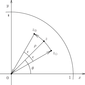
Figure 1: Illustration of the definition of the complex first-order linear low-pass filter within the unit disk of the complex plane. The integral giving the average is taken over the arc of circle from $z_{\ominus}$ to $z_{\oplus}$. The points $z_{\ominus}$, $z_{\oplus}$ and $0$ form a closed contour.

For such functions we may define the action of the first-order linear low-pass filter as an operator acting on the space of real functions, which from the real function $f(\theta)$ produces another real function $f_{\epsilon}(\theta)$ by means of the integral

$$f_{\epsilon}(\theta)=\frac{1}{2\epsilon}\int_{\theta-\epsilon}^{\theta+\epsilon}d\theta^{\prime}\,f\!\left(\theta^{\prime}\right),$$ (1)

which is well-defined at the point $\theta$ so long as the interval $[\theta-\epsilon,\theta+\epsilon]$ does not contain any of the non-integrable singularities of the original function. Since we are on the unit circle, the parameter $\epsilon$ must satisfy $0<\epsilon\leq\pi$. In this paper we will be interested mostly in the limit $\epsilon\to 0$, and in this limit this definition suffices to determine $f_{\epsilon}(\theta)$ at all points except for the non-integrable singular points of $f(\theta)$, that is to say almost everywhere, and strictly everywhere within the domain of definition of $f(\theta)$ itself. The low-pass filter can also be defined in terms of an integration kernel $K_{\epsilon}\!\left(\theta-\theta^{\prime}\right)$,

$$f_{\epsilon}(\theta)=\int_{-\pi}^{\pi}d\theta^{\prime}\,K_{\epsilon}\!\left(\theta-\theta^{\prime}\right)f\!\left(\theta^{\prime}\right),$$

where the kernel is defined as

$$\begin{array}[]{rclcc}K_{\epsilon}\!\left(\theta-\theta^{\prime}\right)&=&{\displaystyle\frac{\displaystyle 1}{\displaystyle 2\epsilon}}&\mbox{for}&\left|\theta-\theta^{\prime}\right|<\epsilon,\\ K_{\epsilon}\!\left(\theta-\theta^{\prime}\right)&=&0&\mbox{for}&\left|\theta-\theta^{\prime}\right|>\epsilon.\end{array}$$

As was shown in [3], this real operator acting on the real functions can be obtained from a corresponding complex operator acting on the inner analytic functions, in the limit from the open unit disk to the unit circle, as follows. Consider an inner analytic function $w(z)$, with $z=\rho\exp(\mbox{\boldmath$\imath$}\theta)$ and $0\leq\rho\leq 1$. We define from it the corresponding filtered complex function $w_{\epsilon}(z)$, using the real angular range parameter $0<\epsilon\leq\pi$, by

$$w_{\epsilon}(z)=-\,\frac{\mbox{\boldmath$\imath$}}{2\epsilon}\int_{z_{\ominus}}^{z_{\oplus}}dz^{\prime}\,\frac{1}{z^{\prime}}\,w\!\left(z^{\prime}\right),$$ (2)

involving an integral over the arc of circle illustrated in Figure 1, where the two extremes are given by

$$z_{\ominus} = z\,{\rm e}^{-\mbox{\boldmath$\imath$}\epsilon}$$

$$= \rho\,{\rm e}^{\mbox{\boldmath$\imath$}(\theta-\epsilon)},$$

$$z_{\oplus} = z\,{\rm e}^{\mbox{\boldmath$\imath$}\epsilon}$$

$$= \rho\,{\rm e}^{\mbox{\boldmath$\imath$}(\theta+\epsilon)}.$$

This definition can be implemented at all the points of the open unit disk. Note that if we make $z\to 0$, the integrand in Equation (2) converges to a finite number, since the Taylor series of $w(z)$ around $z=0$ has no constant term, given that $w(z)$ is an inner analytic function. It follows that in that limit the integral converges to zero, because the domain of integration becomes a single point in the limit. Therefore we conclude that $w_{\epsilon}(0)=0$, which means that the filter reduces to the local identity at $z=0$. Since on the arc of circle we have that $z^{\prime}=\rho\exp(\mbox{\boldmath$\imath$}\theta^{\prime})$ and hence that $dz^{\prime}=\mbox{\boldmath$\imath$}z^{\prime}d\theta^{\prime}$, we may also write the definition of the complex filtered function as

$$w_{\epsilon}(z)=\frac{1}{2\epsilon}\int_{\theta-\epsilon}^{\theta+\epsilon}d\theta^{\prime}\,w\!\left(\rho,\theta^{\prime}\right),$$ (3)

which makes it explicitly clear that what we have here is a simple normalized integral over $\theta$. One can thus see that what we are doing is to map the value of the function $w(z)$ at $z$ to the average of $w(z)$ over the symmetric arc of circle of angular span $2\epsilon$ around $z$, with constant $\rho$. This defines a new complex function $w_{\epsilon}(z)$ at that point.

Repeating what was done in [3] in the context of the old-style inner analytic functions, and since it is a crucial part of our present argument, let us now show that this complex function is in fact analytic, and therefore that it is an inner analytic function according to the newer definition given in [5], since we have already shown that it has the property that $w_{\epsilon}(0)=0$. The definition in Equation (2) has the general form of a logarithmic integral, which is the inverse operation to the logarithmic derivative, as defined and discussed in [2], where the logarithmic primitive of $w(z)$ was defined as the integral

$$w^{-1\!\mbox{\Large$\cdot$}\!}(z)=\int_{0}^{z}dz^{\prime}\,\frac{1}{z^{\prime}}\,w\!\left(z^{\prime}\right),$$

over any simple curve from $z^{\prime}=0$ to $z^{\prime}=z$ within the open unit disk, and where we are using the notation for the logarithmic primitive introduced in that paper. The logarithmic primitive $w^{-1\!\mbox{\Large$\cdot$}\!}(z)$ is an analytic function within the open unit disk, as shown in [2], and it clearly has the property that $w^{-1\!\mbox{\Large$\cdot$}\!}(0)=0$, so that it is an inner analytic function as well. In order to demonstrate the analyticity of $w_{\epsilon}(z)$ we consider the integral over the closed positively-oriented circuit shown in Figure 1, from which it follows that we have

$$\int_{0}^{z_{\ominus}}dz^{\prime}\,\frac{1}{z^{\prime}}\,w\!\left(z^{\prime}\right)+\int_{z_{\ominus}}^{z_{\oplus}}dz^{\prime}\,\frac{1}{z^{\prime}}\,w\!\left(z^{\prime}\right)+\int_{z_{\oplus}}^{0}dz^{\prime}\,\frac{1}{z^{\prime}}\,w\!\left(z^{\prime}\right)=0,$$

due to the Cauchy-Goursat theorem, since the contour is closed and the integrand is analytic on it and within it. It follows that we have

$$\int_{z_{\ominus}}^{z_{\oplus}}dz^{\prime}\,\frac{1}{z^{\prime}}\,w\!\left(z^{\prime}\right)=w^{-1\!\mbox{\Large$\cdot$}\!}(z_{\oplus})-w^{-1\!\mbox{\Large$\cdot$}\!}(z_{\ominus}).$$

Since the logarithmic primitive $w^{-1\!\mbox{\Large$\cdot$}\!}(z)$ is an analytic function within the open unit disk, and since the functions $z_{\ominus}(z)$ and $z_{\oplus}(z)$ are also analytic functions in that domain, it follows that the right-hand side of this equation is an analytic function of $z$ within the open unit disk. We have therefore for the filtered complex function

$$w_{\epsilon}(z)=-\,\frac{\mbox{\boldmath$\imath$}}{2\epsilon}\left[w^{-1\!\mbox{\Large$\cdot$}\!}(z_{\oplus})-w^{-1\!\mbox{\Large$\cdot$}\!}(z_{\ominus})\right],$$ (4)

which shows that $w_{\epsilon}(z)$ is an analytic function as well. Since we have already shown that $w_{\epsilon}(0)=0$, it follows that this complex filtered function is an inner analytic function.

Let us now show that this complex low-pass filter reduces to the real low-pass filter on the unit circle. If we write both the original function $w(z)$ and the filtered function $w_{\epsilon}(z)$ in terms of their real and imaginary parts, the expression in Equation (3) becomes

$$\left[f_{\epsilon}(\rho,\theta)+\mbox{\boldmath$\imath$}\bar{f}_{\epsilon}(\rho,\theta)\right]=\frac{1}{2\epsilon}\int_{\theta-\epsilon}^{\theta+\epsilon}d\theta^{\prime}\,\left[f\!\left(\rho,\theta^{\prime}\right)+\mbox{\boldmath$\imath$}\bar{f}\!\left(\rho,\theta^{\prime}\right)\right],$$

where $\bar{f}_{\epsilon}(\rho,\theta)$ and $\bar{f}(\rho,\theta)$ are the harmonic conjugate functions respectively of $f_{\epsilon}(\rho,\theta)$ and $f(\rho,\theta)$. If we now take the $\rho\to 1$ limit to the unit circle, we get from the real and imaginary parts of this expression

$$f_{\epsilon}(1,\theta) = \frac{1}{2\epsilon}\int_{\theta-\epsilon}^{\theta+\epsilon}d\theta^{\prime}\,f\!\left(1,\theta^{\prime}\right),$$

$$\bar{f}_{\epsilon}(1,\theta) = \frac{1}{2\epsilon}\int_{\theta-\epsilon}^{\theta+\epsilon}d\theta^{\prime}\,\bar{f}\!\left(1,\theta^{\prime}\right),$$

so long as the integration interval on the unit circle does not contain any non-integrable singularities of $w(z)$. Since the real part $f_{\epsilon}(\rho,\theta)$ of $w_{\epsilon}(z)$ tends in the $\rho\to 1$ limit to the real generalized function $f_{\epsilon}(\theta)$ corresponding to the inner analytic function $w_{\epsilon}(z)$, we may conclude that in the $\rho\to 1$ limit the complex filter reduces to the definition of the real filter given in Equation (1), for any real generalized function $f(\theta)=f(1,\theta)$ that can be obtained as the $\rho\to 1$ limit of the real part of an inner analytic function. The same is true for the imaginary part, of course, which converges to the corresponding “Fourier Conjugate” real generalized function, a concept which was defined in [1] and restated in [5].

3 The $\epsilon\to 0$ Limit

In a previously mentioned paper [9] it was shown that the first-order linear low-pass filter, in its real form, tends to the identity operator almost everywhere in the $\epsilon\to 0$ limit. In Section 6 of Appendix A of that paper one can find a simple proof that in this limit the filtered function reproduces the value of the original function whenever that function is continuous, that is

$$\lim_{\epsilon\to 0}f_{\epsilon}(\theta)=f(\theta),$$

which holds at every point where $f(\theta)$ is continuous. At isolated points of discontinuity where the two lateral limits of the original function to the point of discontinuity exist, the filtered function converges, in the $\epsilon\to 0$ limit, to the average of the two lateral limits, as shown in Section 7 of that same Appendix,

$$\lim_{\varepsilon\to 0}f_{\varepsilon}(\theta_{0})=\frac{1}{2}\left({\cal L}_{\oplus}+{\cal L}_{\ominus}\right),$$

where

$${\cal L}_{\oplus} = \lim_{\hskip 5.60002pt\theta\to\theta_{0+}}f(\theta),$$

$${\cal L}_{\ominus} = \lim_{\hskip 5.60002pt\theta\to\theta_{0-}}f(\theta).$$

When the two limits coincide, and therefore the original function is continuous at the point $\theta_{0}$, this of course reduces to the previous property. At isolated points of non-differentiability where the two lateral limits to that point of the derivative of the original function exist, the derivative of the filtered function converges, in the $\epsilon\to 0$ limit, to the average of these two lateral limits, as shown in Section 8 of that same Appendix,

$$\lim_{\varepsilon\to 0}\frac{df_{\varepsilon}}{d\theta}(\theta_{0})=\frac{1}{2}\left({\cal L^{\prime}}_{\oplus}+{\cal L^{\prime}}_{\ominus}\right),$$

where

$${\cal L^{\prime}}_{\oplus} = \lim_{\hskip 5.60002pt\theta\to\theta_{0+}}\frac{df}{d\theta}(\theta),$$

$${\cal L^{\prime}}_{\ominus} = \lim_{\hskip 5.60002pt\theta\to\theta_{0-}}\frac{df}{d\theta}(\theta).$$

Of course, this implies that, at points where the function $f(\theta)$ is differentiable, the derivative of the filtered function converges, in the $\epsilon\to 0$ limit, to the derivative of the original function. From all this we may conclude that, so long as there is only a finite number of singular points, or at most an infinite but zero-measure set of such points, in the $\epsilon\to 0$ limit the real filter becomes the identity operator almost everywhere.

In addition to this, one can easily prove that the corresponding complex filter always becomes exactly the identity operator in the $\epsilon\to 0$ limit, within the open unit disk. This was commented on in [3], but since it is quite crucial to our current argument let us repeat the demonstration here. We can see this from the complex-plane definition in Equation (4). If we consider the variation of $\theta$ between the extremes $z_{\oplus}$ and $z_{\ominus}$, which is given in terms of the parameter $\epsilon$ by $\delta\theta=2\epsilon$, and we take the $\epsilon\to 0$ limit of that expression, we get

$$\lim_{\epsilon\to 0}w_{\epsilon}(z) = -\mbox{\boldmath$\imath$}\,\lim_{\epsilon\to 0}\frac{w^{-1\!\mbox{\Large$\cdot$}\!}(z_{\oplus})-w^{-1\!\mbox{\Large$\cdot$}\!}(z_{\ominus})}{2\epsilon}$$

$$= -\mbox{\boldmath$\imath$}\,\lim_{\delta\theta\to 0}\frac{w^{-1\!\mbox{\Large$\cdot$}\!}(z_{\oplus})-w^{-1\!\mbox{\Large$\cdot$}\!}(z_{\ominus})}{\delta\theta}$$

$$= z\lim_{\delta z\to 0}\frac{w^{-1\!\mbox{\Large$\cdot$}\!}(z_{\oplus})-w^{-1\!\mbox{\Large$\cdot$}\!}(z_{\ominus})}{\delta z},$$

where we used the fact that in the limit $\delta z=\mbox{\boldmath$\imath$}z\delta\theta$. Since we have that $\delta z=z_{\oplus}-z_{\ominus}$, we see that the limit above defines the logarithmic derivative of $w^{-1\!\mbox{\Large$\cdot$}\!}(z)$. In addition to this, since that function is analytic in the open unit disk, the limit necessarily exists. Therefore, we have

$$\lim_{\epsilon\to 0}w_{\epsilon}(z) = z\,\frac{d}{dz}w^{-1\!\mbox{\Large$\cdot$}\!}(z)$$

$$= w(z),$$

since we have here the logarithmic derivative of the logarithmic primitive, and the operations of logarithmic differentiation and logarithmic integration are the inverses of one another, as shown in [2]. We see, therefore, that this property within the open unit disk is stronger than the corresponding property on the unit circle, since in this case we have exactly the identity in all cases, while in the real case we had only the identity almost everywhere. We have therefore that, for all inner analytic functions $w(z)$,

$$\lim_{\epsilon\to 0}w_{\epsilon}(z)=w(z),$$

which holds in the whole open unit disk. Since every inner analytic function, filtered or not, corresponds to a real generalized function on the unit circle in the $\rho\to 1$ limit, defined at all points where this limit exists, the one-parameter family of inner analytic functions $w_{\epsilon}(z)$ corresponds to a one-parameter family of real generalized functions $f_{\epsilon}(\theta)$ on the unit circle. It is therefore clear that as $w_{\epsilon}(z)$ approaches $w(z)$ in the $\epsilon\to 0$ limit, so does $f_{\epsilon}(\theta)$ approach $f(\theta)$ in that same limit, at all points of the unit circle where the $\rho\to 1$ limit exists, that is, at least almost everywhere.

4 The Classification

The first-order low-pass filter can now be used to define a classification of generalized functions. In order for the filter to be applicable, and therefore for the classification to be feasible, the generalized functions must be locally integrable almost everywhere, but they do not have to be integrable on the whole domain. Observe, moreover, that we do not have to assume that the generalized functions which we start with in this argument were defined as $\rho\to 1$ limits of corresponding inner analytic functions. Therefore, given a generalized function $f(\theta)$ which is locally integrable almost everywhere on the unit circle, irrespective of whether or not it was defined as the $\rho\to 1$ limit of an inner analytic function, we say that it is a combed function if it is true that

$$f(\theta)=\lim_{\epsilon\to 0}f_{\epsilon}(\theta),$$ (5)

where this recovery of the original function from the $\epsilon\to 0$ limit of the filtered function holds everywhere. Otherwise we say that the generalized function is a ragged function. The results obtained in [9] and discussed in the previous section now imply that any continuous function is a combed function. We may consider adopting a corresponding complex definition, using the corresponding criterion for the inner analytic functions within the open unit disk. Therefore we may classify an inner analytic function as combed if it satisfies the condition that

$$w(z)=\lim_{\epsilon\to 0}w_{\epsilon}(z),$$ (6)

where the recovery of the original function from the $\epsilon\to 0$ limit of the filtered function holds everywhere within the open unit disk. However, we showed in the previous section that this is the case for all inner analytic functions. This means that every inner analytic function is combed within the open unit disk.

Since the complex low-pass filter reduces to the real low-pass filter on the unit circle, it follows at once that all the generalized functions obtained as limits to the unit circle of the real parts of inner analytic functions within the open unit disk are combed functions, which we will refer to as “combed generalized functions”. While this simply reproduces the previously obtained results [9] for the case of continuous real functions on the unit circle, it also means that the Dirac delta “function” is a combed generalized function, which is quite a remarkable fact. In this particular case it is not difficult to verify this fact directly, but from the same result expressed by Equation (6) it follows that this is also true for all the derivatives of the delta “function”, of all orders, which is not so simple and immediately apparent a fact.

Here is a simple direct proof that the delta “function” is a combed generalized function. Consider a delta “function” $\delta(\theta-\theta_{0})$ centered at $\theta_{0}$. It is not difficult to verify by direct calculation that the real filter with parameter $\epsilon$, if applied to this generalized function, produces a unit-integral rectangular pulse of width $2\epsilon$ and height $1/(2\epsilon)$ centered at that same point. As one decreases $\epsilon$, the $\epsilon\to 0$ limit of this one-parameter family of rectangular pulses is one of the many ways commonly used as a definition of the delta “function”. Therefore one recovers the delta “function” in the $\epsilon\to 0$ limit, thus showing that the delta “function” is a combed generalized function.

A similar argument can be constructed for the first derivative of the delta “function”, in which one must use some of the properties of the delta “function” itself, and the fact that the derivative of the integration kernel $K_{\epsilon}\!\left(\theta-\theta^{\prime}\right)$ contains a pair of delta “functions”. However, in this case it is much simpler to establish that the derivative of the delta “function” is a combed generalized function by simply relying on the fact that it is the $\rho\to 1$ limit of an inner analytic function, as was shown in [5]. The same argument is valid, with equal ease, for all the derivatives of the delta “function”, of arbitrarily high orders.

It is also easy to see by direct calculation that any function with a few isolated step-type discontinuities where the two lateral limits exist, and which is otherwise continuous, is a combed function, so long as at the points of discontinuity the function is defined as the average of the two lateral limits. Note that this is the value to which the Fourier series of the function converges, if that series is convergent at all. Once again, this result can be easily derived from the fact that functions such as the ones just described can be obtained as the $\rho\to 1$ limits of the real parts of the corresponding inner analytic functions.

4.1 Properties of Combed Functions

Although the class of combed function includes many singular objects such as the delta “function” and at least some locally non-integrable functions, the generalized functions within the set have a significant collection of common properties that considerably simplifies their handling. Note that this is a large set of objects including many singular ones of common use in physics, since combed function can be non-differentiable, discontinuous, and may diverge to infinity at singular points, which may or may not be integrable ones. For the purposes of this section let us limit ourselves to the case in which the combed generalized functions are integrable. This will make it easier for us to list their main common properties, most of which have been demonstrated before. The detailed extension of these properties to the complete set of combed generalized functions is therefore postponed to some future opportunity.

• To start with, combed functions have no finite-spike singularities. In fact, any pathologies that do not have a definite non-zero effect on the integral of the function, such as finite discontinuities on a zero-measure subset of the domain, are simply eliminated by the application of the low-pass filter.

• Since it is the $\epsilon\to 0$ limit of a filtered function, every combed function assumes at every given point the value given by the average of the two lateral limits of the original function to that point, so long as these limits exist,

  $$\frac{{\cal L}_{\oplus}+{\cal L}_{\ominus}}{2},$$

  where

  $${\cal L}_{\oplus} = \lim_{\hskip 5.60002pt\theta\to\theta_{0+}}f(\theta),$$

  $${\cal L}_{\ominus} = \lim_{\hskip 5.60002pt\theta\to\theta_{0-}}f(\theta),$$

  which in particular holds at all isolated discontinuities where the two lateral limits exist. Note that, since in the neighborhoods at the two sides of $\theta_{0}$, where $f(\theta)$ is continuous, the $\epsilon\to 0$ limit of $f_{\epsilon}(\theta)$ reproduces $f(\theta)$, these two lateral limits of $f(\theta)$ coincide with the two corresponding lateral limits of $f_{\epsilon}(\theta)$ in the $\epsilon\to 0$ limit.

• Every combed function $f(\theta)$ has a well-defined and unique sequence of Taylor-Fourier coefficients, from which it can be recovered strictly everywhere within its domain of definition. From the sequence of Taylor-Fourier coefficients one can always construct the corresponding inner analytic function $w(z)$. The combed real function is always given by the $\rho\to 1$ limit of the real part of its corresponding inner analytic function,

  $$f(\theta)=\lim_{\rho\to 1}\Re[w(z)],$$

  everywhere within that domain, even if the Fourier series of that real function diverges everywhere.

• If the Fourier series of a combed function converges at all, then it converges to that combed function everywhere in its domain of definition.

• If the Fourier series of a combed function diverges, and so long as there is at most a finite number of dominant singularities of the corresponding inner analytic function on the unit circle, as they were defined in [2], it is possible to devise other expressions involving trigonometric series that converge to the real function, and that do so as fast as one may wish. We call these alternative trigonometric series “center series”, and the algorithm to construct them is explained in [2].

• Every combed function is the smoothest member of the class of zero-measure equivalent functions that it belongs to, as was discussed in Appendix C of [4]. Given another member of that class, which is therefore a ragged function, there is no difficulty in “combing” it, that is in finding the combed function from which it differs only by a zero-measure function.

• A ragged function can be combed by any one of the following methods: application to it of the low-pass filter in the $\epsilon\to 0$ limit; construction of its Fourier series, if convergent, and therefore of the limiting function of that series; construction of an expression containing an alternative trigonometric series, if the Fourier series fails to converge, and therefore of the limiting function of that alternative series; construction of its inner-analytic function and therefore of the limit of the real part of that complex function to the unit circle.

In any given setting, if one limits the set of relevant real functions to be discussed to combed generalized functions, then the use of the very characteristic “almost everywhere” arguments in the harmonic analysis of the functions become more sparse and better focused on the relevant features of the functions. The possible exceptional points of the “almost everywhere” arguments become only those singular points on the unit circle that are brought about by the construction of the corresponding inner analytic functions.

5 Sufficiency for Physics

In this section we argue, in a few different but related ways, that combed generalized functions suffice to describe all physics. We mean this statement to include all classical physics and all observables quantities in quantum mechanics and quantum field theory. Note that we do not argue that the use of combed generalized functions is necessary, only that it is sufficient. There are a few ways in which one can argue this case, which we will present in what follows. It should be noted in passing that the limitation of the functions to the interval $[-\pi,\pi]$ is of no consequence for this discussion of the physics applications, as shown in Appendix A.

5.1 Fundamental Limitations on Precision

Perhaps one of the most basic ways to argue the case starts from the fundamental fact that all physical measurements of quantities that vary almost continuously are necessarily made within finite and non-zero errors. The representation of nature provided by physics is always an approximate one. All physical measurements, as well as all theoretical calculations related to them, of quantities which are represented by continuous variables, can only be performed with finite amounts of precision, that is, within finite and non-zero errors.

In fact, not only this is true in practice, both experimentally and theoretically, but with the advent of relativistic quantum mechanics and quantum field theory, it became a limitation in principle as well. This is so because in its most fundamental aspect all particles in nature are represented by fields, in the sense that the particles are just energetic excitations of these fields. For finite particle energies the wavelengths of these fields are finite and non-zero. Since it is not possible to localize the particles with an accuracy that falls below the length scales defined by those wavelengths, it follows that it is never possible to measure the position of particles, or the dimensions of objects constructed out of these particles, with mathematically perfect precision.

The use of real functions in physics is meant to be for the representation of relations between physical variables that vary almost continuously. If we assume that the physical quantities are observable, then they can at best be measured or prepared (that is, set) within finite and non-zero errors. A relation such as $y=f(x)$ where both $x$ and $y$ are observable means that a finite-spike discontinuity in the function cannot have any physical meaning. In order to detect such a spike in $y$ it would be necessary to measure or prepare $x$ with infinite precision, which is never possible, not only in practice but in principle. Therefore, there is no possible physical meaning to ragged functions containing any such finite-spike discontinuities.

5.2 Representability in Momentum Space

Another argument for the sufficiency of combed generalized functions for the representation of physical quantities uses the representation of the physics in momentum space. This representation is mathematically equivalent to the use of the Fourier coefficients of the real generalized functions as a way to represent those functions. The representation of the physics in momentum space can always be constructed, and it is often found to have a more direct and profound physical meaning than the original representation in position space. This is so, in no small measure, because the momentum-space modes that arise in this way represent distributed quantities, and do not involve any attempt at localizing any objects with mathematically perfect precision. Examples of this are everywhere, ranging from normal modes of vibration in classical and quantum physics to the construction of states of particles in quantum field theory.

The functions giving the solutions of physical problems are usually solutions of boundary value problems of partial differential equations. One of the most common and standard ways to solve such problems is via the representation of the solutions in momentum space, which is equivalent to the representation of the functions involved by their sequences of Fourier coefficients. It follows at once that all solutions obtained in this way are combed generalized functions. As was shown in the appendices of [9], the mere application of the low-pass filters will usually improve rather than harm the representation of the physics by the mathematics, even if the $\epsilon\to 0$ limit is not actually taken at the end of the day. Moreover, when it is taken, since we are taking the $\epsilon\to 0$ limit of a filtered function, we always end up with a combed function.

Since two zero-measure equivalent generalized functions have exactly the same set of Fourier coefficients, and thus cannot be distinguished from each other by the use of those coefficients, it follows that if the physics can be represented in momentum space at all, then the two zero-measure equivalent generalized functions must represent exactly the same physics. If we add to this the fact that the Fourier series, if convergent at all, always converges to the combed function belonging to that class of zero-measure equivalent generalized functions, then we must conclude that the combed generalized functions are sufficient for the representation of the physics involved. The same conclusion can be drawn for every other way used to represent a generalized function by its sequence of Fourier coefficients, such as through the corresponding inner analytic function or through alternative expressions involving center series, which are just other trigonometric series. This is so because all such method of representation always produce combed functions.

5.3 Representability by Differential Equations

As a third argument for the sufficiency of combed generalized functions for physics, we may go back to the fact that physics is often expressed by second-order differential equations. Given an arbitrary second-order differential equation to be satisfied by a real function $f(\theta)$, if we are to consider the derivatives involved in the standard way, then the function $f(\theta)$ must necessarily be twice-differentiable, and therefore differentiable and continuous. Since every continuous function is a combed function, this implies that $f(\theta)$ must be a combed function, and in this case also a normal real function. However, just as in the standard Schwartz theory of distributions, the introduction of generalized functions represented by inner analytic functions allows us to generalize the concept of differentiability and hence to enlarge the scope of the differential equations.

If a real function $f(\theta)$ is not strictly differentiable at a given singular point, we may still be able to uniquely attribute a value to its derivative at that point, by the following sequence of operations: first we go to the open unit disk of the complex plane and take the inner analytic function $w(z)$ associated to that real function; second, since the inner analytic function is always differentiable, we then take its logarithmic derivative, which produces another inner analytic function within the open unit disk; finally, we take the limit of the real part of this new complex analytic function to the singular point on the unit circle; it that limits exists (as it often will), we attribute that value to the derivative of the original function at the singular point.

This can be further generalized, in case the limit to the unit circle does not exist in a strict sense, by the global attribution of a singular generalized function as the derivative of a strictly non-differentiable function. In this way one may state, for example, that the derivative of a function with a step-type singularity of height one at a certain point contains a delta “function” centered at that point. From the point of view of this more general definition of the derivative, all combed generalized functions are differentiable, and in fact infinitely differentiable, just as in the standard Schwartz theory of distributions. We are therefore able to consider arbitrary generalized functions as possible solutions of differential equations, so long as we reinterpret these equations in terms of generalized derivatives.

Note that this extension of the scope of differential equations, if executed via the representation of the generalized functions by inner analytic functions, is done without leaving the realm of combed objects, which in this case are combed generalized functions. Therefore, once again we may argue that combed generalized functions suffice for the description of physics.

6 Conclusions

We have shown that the real first-order low-pass filter, if taken in the $\epsilon\to 0$ limit, can be used to classify all possible generalized functions defined within a closed real interval into two disjoint classes, a class of combed generalized functions and a complementary class of ragged generalized functions. Although the first one contains, by and large, more regular members and less singular members than the second, the classification is not based simply on smoothness, since both classes do contain singular members. In addition to this, given any ragged function, there always is a corresponding combed function, from which it differs only by a zero-measure function. In this way, the concept suggests itself of the process of “combing” ragged functions. They can be “combed” so long as they can be characterized by a sequence of Taylor-Fourier coefficients, regardless of the convergence properties of the corresponding Fourier series. In all cases there are several ways in which this “combing” can be accomplished, including some that are algorithmically sound and useful.

We have also shown that the class of combed functions contains all those generalized functions that can be obtained as the $\rho\to 1$ limits of inner analytic functions. This same class is also that which contains the limiting generalized functions of all convergent Fourier series, as well as the limiting generalized functions obtained from all convergent center series built from the sequences of Fourier coefficients of real generalized functions. At this time we are not able to ascertain whether of not all combed generalized functions can be represented by inner analytic functions. This is so because although we have shown in [5] that the set of inner analytic functions includes representations of at least some locally non-integrable functions, we do not yet know whether or not it contains all of them. In other words, it is an open question whether or not all generalized functions which are locally integrable almost everywhere are the derivatives of some order of integrable generalized functions, and therefore can be represented by inner analytic functions in the way presented in [5], using the extended Taylor-Fourier coefficients introduced there.

It is interesting that, if one does not actually take the $\rho\to 1$ limit, but just gets sufficiently close to the unit circle to decrease sufficiently the errors involved, then one can draw the conclusion that, given any level of precision, there is an analytic real function that represents the physics within that precision. If one considers the restriction of the real part of any given inner analytic function to the circle of radius $\rho=1-\delta$, for some arbitrarily small but non-zero $\delta$, it becomes clear that this restriction is an analytic real function, since it is infinitely differentiable everywhere. If the limiting function represents some given physics within some error level and there are no hard singularities (where the representation must break down anyway), then the analytic real function obtained by this restriction with a sufficiently small $\delta$ represents the same physics as the function obtained in the $\rho\to 1$ limit, within the same error level. We may thus conclude that, given any real function that represents some physics within the finite and non-zero errors that are made inevitable by the fundamental physical limitations on the determination of all physical quantities that vary almost continuously, there is always a real analytic function arbitrarily close to it, that represents the same physics equally well, that is within the same level of precision.

The same conclusion can be reached if we start from the fact that the real functions that carry physical meaning in physics applications can also be represented by series in a basis of orthogonal functions, which is often the case when the functions are solutions of boundary value problems involving partial differential equations. Besides the Fourier basis of functions, this includes such commonly used bases as those formed by Legendre polynomials and those formed by Bessel functions of various types, among many others. One property that all these bases share is that they are infinite but discrete sets of analytic functions. If the series representing the functions are convergent, then the real functions can be represented by partial sums of the series within an arbitrarily given finite level of precision. However, these partial sums are finite sums of analytic functions and therefore are themselves analytic. In all these cases it follows that the physics can always be represented by analytic functions arbitrarily well, that is, within the finite and non-zero errors that are mandated by the fundamental physical limitations on the determination of all physical quantities that vary almost continuously.

As a final thought, one can pose the question of whether or not all solutions to linear partial differential equations are necessarily combed generalized functions. We believe that the right way to interpret this question is to ask whether or not there is an even more general way to extend the scope of differential equations that the transition from normal functions to generalized functions, and from normal derivatives to generalized derivatives, defined as we do here. So far as can be currently ascertained, this seems to be an open question.

Appendix A Appendix: Reduction of Domain Intervals

The fact that we discuss the properties of real functions only within the interval $[-\pi,\pi]$ is not a limitation from the physics point of view. It is easy to show that all situations in physics application can be reduced to this interval. Let us consider a physical variable $x$ within the closed interval $[a,b]$, and let $g(x)$ be a real function describing some physical quantity within that interval. The size of the interval does not matter. For example, if $x$ is a measure of length, the interval could be the size of a small resonant cavity or it could be the size of the galaxy. In any case it is still a closed interval. The same is true if $x$ represents an energy, since it is always true that only limited amounts of energy are available for any given experiment or realistic physical situation. So long as $x\in[a,b]$, regardless of the magnitude or physical nature of the dimensionfull physical variable $x$, we can rescale it to fit within $[-\pi,\pi]$. It is a simple question of making a change of variables, by defining the new dimensionless variable

$$\theta=2\pi\,\frac{x-a}{b-a}-\pi,$$

so that $\theta\in[-\pi,\pi]$. The inverse transformation is given by

$$x=\frac{b-a}{2\pi}\,\theta+\frac{b+a}{2}.$$

The function $g(x)$ can now be transformed into a function $f(\theta)$,

$$g(x)=f(\theta),$$

where $f(\theta)$ describes the same physics as $g(x)$. Let us now consider the transformation of the first-order low-pass filter from one system of variables to the other. Given a value of $\theta$, if we vary it by $\epsilon$, we have a corresponding variation of $x$, which we will call $\varepsilon$. It then follows that we have a relation between $\varepsilon$ and $\epsilon$,

$$x\pm\varepsilon = \frac{b-a}{2\pi}\,(\theta\pm\epsilon)+\frac{b+a}{2}$$

$$= \left(\frac{b-a}{2\pi}\,\theta+\frac{b+a}{2}\right)\pm\frac{b-a}{2\pi}\,\epsilon$$

$$= x\pm\frac{b-a}{2\pi}\,\epsilon\;\;\;\Rightarrow$$

$$\varepsilon = \frac{b-a}{2\pi}\,\epsilon.$$

The limit $\epsilon\to 0$ is now seen to be clearly equivalent to the limit $\varepsilon\to 0$, and the definition of the filtered function $f_{\epsilon}(\theta)$ has a counterpart $g_{\varepsilon}(x)$,

$$f_{\epsilon}(\theta) = \frac{1}{2\epsilon}\int_{\theta-\epsilon}^{\theta+\epsilon}d\theta^{\prime}\,f(\theta^{\prime})\;\;\;\Rightarrow$$

$$g_{\varepsilon}(x) = \frac{1}{2\varepsilon}\int_{x-\varepsilon}^{x+\varepsilon}dx^{\prime}\,g(x^{\prime}).$$

It follows that if $f(\theta)$ is a combed function and we thus have that

$$f(\theta)=\lim_{\epsilon\to 0}f_{\epsilon}(\theta),$$

then we also have that

$$g(x)=\lim_{\varepsilon\to 0}g_{\varepsilon}(x),$$

so that $g(x)$ is also a similarly combed function. We may thus conclude that it suffices to consider and discuss only the set of combed functions within $[-\pi,\pi]$.

References

- [1] J. L. deLyra, “Fourier Theory on the Complex Plane I – Conjugate Pairs of Fourier Series and Inner Analytic Functions”, arXiv: 1409.2582.
- [2] J. L. deLyra, “Fourier Theory on the Complex Plane II – Weak Convergence, Classification and Factorization of Singularities”, arXiv: 1409.4435.
- [3] J. L. deLyra, “Fourier Theory on the Complex Plane III – Low-Pass Filters, Singularity Splitting and Infinite-Order Filters”, arXiv: 1411.6503.
- [4] J. L. deLyra, “Fourier Theory on the Complex Plane IV – Representability of Real Functions by their Fourier Coefficients”, arXiv: 1502.01617.
- [5] J. L. deLyra, “Fourier Theory on the Complex Plane V – Arbitrary-Parity Real Functions, Singular Generalized Functions and Locally Non-Integrable Functions”, arXiv: 1505.02300.
- [6] See, for example, R. V. Churchill and J. W. Brown, “Complex Variables and Applications”, McGraw-Hill Book Co., 1995, and the references therein.
- [7] See, for example, R. V. Churchill and J. W. Brown, “Fourier Series and Boundary Value Problems”, McGraw-Hill Book Co., 2011, and the references therein.
- [8] L. Schwartz, “Théorie des Distributions”, 1-2, Hermann, Paris, (1951). M. J. Lighthill, “Introduction to Fourier Analysis and Generalized Functions”, Cambridge University Press, (1959). ISBN 0-521-09128-4.
- [9] J. L. deLyra, “Low-Pass Filters, Fourier Series and Partial Differential Equations”, arXiv: 1410.8710.
- [10] W. Rudin, “Principles of Mathematical Analysis”, McGraw-Hill, third edition, 1976; ISBN-13: 978-0070542358, ISBN-10: 007054235X. H. Royden, “Real Analysis”, Prentice-Hall Inc., third edition, 1988; ISBN-13: 978-0024041517, ISBN-10: 0024041513.