Chemical Abundances in the PN Wray16-423 in the Sagittarius Dwarf Spheroidal Galaxy: Constraining the Dust Composition

Abstract

We performed a detailed analysis of elemental abundances, dust features, and polycyclic aromatic hydrocarbons (PAHs) in the C-rich planetary nebula (PN) Wray16-423 in the Sagittarius dwarf spheroidal galaxy, based on a unique dataset taken from the Subaru/HDS, MPG/ESO FEROS, HST/WFPC2, and Spitzer/IRS. We performed the first measurements of Kr, Fe, and recombination O abundance in this PN. The extremely small [Fe/H] implies that most Fe atoms are in the solid phase, considering into account the abundance of [Ar/H]. The Spitzer/IRS spectrum displays broad 16-24 $\mu$m and 30 $\mu$m features, as well as PAH bands at 6-9 $\mu$m and 10-14 $\mu$m. The unidentified broad 16-24 $\mu$m feature may not be related to iron sulfide (FeS), amorphous silicate, or PAHs. Using the spectral energy distribution model, we derived the luminosity and effective temperature of the central star, and the gas and dust masses. The observed elemental abundances and derived gas mass are in good agreement with asymptotic giant branch nucleosynthesis models for an initial mass of 1.90 M_⊙ and a metallicity of $Z$=0.004. We infer that respectively about 80 %, 50 %, and 90 % of the Mg, S, and Fe atoms are in the solid phase. We also assessed the maximum possible magnesium sulfide (MgS) and iron-rich sulfide (Fe50S) masses and tested whether these species can produce the band flux of the observed 30 $\mu$m feature. Depending on what fraction of the sulfur is in sulfide molecules such as CS, we conclude that MgS and Fe50S could be possible carriers of the 30 $\mu$m feature in this PN.

1 Introduction

Planetary nebulae (PNe) represent the final stage in the evolution of initially $\sim$1-8 M_⊙ stars. During their evolution, these mass stars eject a large amount of their mass into circumstellar shells via strong stellar winds. Eventually, the ejecta blend with interstellar media (ISM). The evolution history of the progenitors is imprinted in the central stars of PNe (CSPNe), in the atomic gas, dust, and molecule-rich circumstellar shells. Using the emission lines of gas and thermal radiation from dust grains, one can simultaneously obtain abundances of elements and dust, as well as the ejected gas/dust masses from the PN progenitors. An investigation of these materials provides insight into stellar evolution and the ISM material-recycling mechanism of host galaxies. Thus, PNe provide a unique laboratory for the study of stellar and galaxy evolution.

Elemental abundances, the luminosities of CSPNe, and gas and dust masses are essential to understanding stellar and galaxy evolution; the latter three parameters are more accurately obtained through observations of extragalactic PNe, rather than Galactic PNe, because the distance is well determined. Currently, there are over 4,200 known extragalactic PNe (from Table 1 of Reid, 2012). In the galaxy that is nearest to us (24.8$\pm$0.8 kpc; Kunder & Chaboyer, 2009), the Sagittarius dwarf spheroidal galaxy (Sgr dSph), four PNe have been confirmed to date; BoBn1, StWr2-21, Hen2-436, and Wray16-423 (Walsh et al., 1997; Dudziak et al., 2000; Zijlstra et al., 2006a; Kniazev et al., 2008; Otsuka et al., 2008, 2010, 2011).

Sgr dSph PNe offer obvious advantages over other extragalactic PNe in terms of the study of stellar evolution, such as those found in Magellanic Clouds (MCs); Sgr dSph PNe are closer to us and therefore appear brighter than other extragalactic PNe, allowing the detection of rare elements such as neutron ($n$)-capture elements. The final yields of neon and $n$-capture elements are largely concerned with the ¹³C pocket region that forms in the He-rich intershell during the thermal-pulse asymptotic giant branch (AGB) phase. The extent of the ¹³C pocket is an important parameter in AGB nucleosynthesis models; however, it remains unconstrained. An assessment of $n$-capture and neon abundances, and the progenitor mass derived from Sgr dSph PNe could be used to test the ¹³C pocket mass adopted in AGB models.

The C/O ratio is an important parameter with regard to CSPN and nebula characterisation and initial mass constraints. The C and O abundances using recombination lines (RLs) are sometimes larger than those using collisionally excited lines (CELs; e.g., see Liu, 2006, for details). Moreover, the discrepancy factor between the RL and CEL abundances is generally different for O and for C (e.g., see Wang & Liu, 2007). As a consequence, the C/O ratio determined from dividing the RL C abundance by the CEL O abundance might not be indicative of the actual C/O ratio. Therefore, we should at the very least determine the C/O ratios using the same type of emission lines. According to Delgado-Inglada & Rodríguez (2014), the uncertainty of the RL C/O ratio ($\pm$0.06 dex) is considerably smaller than that of the CEL C/O ratio ($\pm$0.2 dex). An important factor of the CEL C/O uncertainty is the normalization between UV and optical fluxes since CEL C abundances are determined using the UV $[$C iii $\lambda\lambda$1906/09 Å lines whereas we measure the CEL O abundances using the optical [O iii] $\lambda\lambda$4959/5007 Å and [O ii] $\lambda\lambda$3726/29 Å. By using C and O RLs in the optical, we do not have to worry about this difficult flux normalization and one can simultaneously determine C and O abundances and then the C/O ratio, as performed in Sgr dSph PNe BoBn1 (Otsuka et al., 2010) and Hen2-436 (Otsuka et al., 2011).

The Hubble Space Telescope (HST) can resolve the central stars of Sgr dSph PNe, as reported in Zijlstra et al. (2006a). Therefore, the luminosities of the CSPNe can be measured directly, without the need for empirical methods. The mass of the progenitor star can be estimated by plotting the measured luminosity and temperature of the CSPN on theoretical post-AGB evolution tracks. Thus, using this approach, the observed elemental abundances and gas mass can be compared to predicted values from AGB nucleosynthesis models.

Previously, we carried out multiwavelength observational studies of the Sgr dSph PNe BoBn1 (Otsuka et al., 2010) and Hen2-436 (Otsuka et al., 2011). While all Sgr dSph PNe are metal-poor (Walsh et al., 1997; Dudziak et al., 2000; Zijlstra et al., 2006a), BoBn1 is extremely metal-poor when comparing to Hen2-436 or Wray16-243 (Otsuka et al., 2015; Zijlstra et al., 2006a; Kniazev et al., 2008). Our study on chemical abundances and dust in these Sgr dSph PNe has provided us with much information on PNe and their progenitor’s evolution. Otsuka et al. (2010) measured the rare $n$-capture elements Xe and Ba abundances for first time in extragalactic PNe. Based on the abundance pattern of BoBn1, they proposed that the progenitor might be a binary. Otsuka et al. (2011) measured the $n$-capture Kr abundance for the first time in Hen2-436 and found that the abundance pattern is very similar to that of Wray16-423. Both studies furthermore also derived dust masses and discussed the dust production in metal-poor environments. In this paper, we focus on the Sgr dSph PN Wray 16-423.

Wray16-423 was discovered near the core of the Sgr dSph by Zijlstra & Walsh (1996), based on direction and radial velocities. Ibata et al. (1995) reported an average heliocentric radial velocity for the Sgr dSph of 140$\pm$2 km s^-1, with an intrinsic velocity dispersion of 11.4$\pm$0.7 km s^-1 (Ibata et al., 1997). The radial velocity of Wray16-423 was determined to be +133.1$\pm$2 km s^-1 by Zijlstra & Walsh (1996). The elemental abundances of the nebula and the luminosity and effective temperature of the CSPN were calculated by Walsh et al. (1997); these values were refined by the photoionisation models of Dudziak et al. (2000), Gesicki & Zijlstra (2003), and Zijlstra et al. (2006a, see Table 4 and Section 3.4 for a comparison of these values). Dudziak et al. (2000) calculated the respective C and O abundances from the C RLs and the O CELs. The C/O ratio using the same type of emission lines is still unknown. Dudziak et al. (2000) expected an [Fe/H] abundance of $\sim$–0.5, although they did not report the detection of Fe lines. Zijlstra et al. (2006a) determined the magnitude of the CSPN to be $m_{V}$=18.85$\pm$0.20, based on HST/F547M measurements. However, this estimate seems to be too bright. Indeed, assuming a spectral energy distribution defined by an $m_{V}$=18.85 CSPN and adopting an effective temperature of 107 000 K (Zijlstra et al., 2006a), the luminosity $L_{\ast}$ should be $\sim$12 600 L_⊙. However, this does not match their estimated value of $L_{\ast}$=4350 L_⊙ obtained using a photoionisation model. This discrepancy and a revision of the CSPN magnitude is discussed in Section 2.4.

Stanghellini et al. (2012) reported that the Spitzer mid-infrared spectrum of Wray16-423 displays carbonous dust features. As we report later, the broad 30 $\mu$m feature is seen in this PN. The broad 30 $\lambda$m feature has been found in many C-rich objects. However, the carrier of the broad 30 $\mu$m feature is unidentified; Hony et al. (2002a) proposed that the feature originates from magnesium sulfide (MgS) whose shapes can be described by a continuous distribution of ellipsoids (CDE). Since then, CDE MgS grains have been the major candidate for the 30 $\mu$m feature (e.g., Zijlstra et al., 2006b; Sloan et al., 2014). However, the recent study of Zhang et al. (2009) casts doubt on this identification for the 30 $\mu$m feature. They demonstrated that the MgS mass formed from the available S atoms, could not account for the observed strength of the 30 $\mu$m feature in the Galactic proto-PN HD56126, even if all the dust grains existed as MgS. CDE iron-rich sulphide, such as Mg_0.5Fe_0.5S (Fe50S), also show a broad feature around 30 $\mu$m, similar to the CDE MgS feature (Messenger et al., 2013). Using the data of Wray16-423, we can test whether the strength of the 30 $\mu$m feature can be explained by thermal emission from the available MgS or Fe50S grains. Since the distance to Wray16-423 is well determined, one can directly determine the luminosity of the CSPN as the gas and dust heating source and set the size of the dusty nebula. Therefore, the solid phase Mg, S, and Fe masses and the MgS and Fe50S grain masses would be more credible by using the accurately measured Mg, S and Fe abundances.

For the above reasons, we performed a detailed spectroscopic analysis of Wray16-423 based on multiwavelength data taken from Subaru/HDS, MPG ESO/FEROS, Spitzer/IRS, and HST/WFPC2: (1) to determine and refine nebular elemental abundances, in particular, the C and O recombination abundances and Fe and slow $n$-capture process ($s$-process) elements; (2) to investigate dust features and PAH bands and compare these among LMC PNe; (3) to derive the physical conditions of the CSPN, gas, and dust by constructing the spectral energy distribution (SED) model using the radiative transfer code Cloudy (Ferland et al., 1998); (4) to estimate the progenitor mass by comparing the observed elemental abundances and estimated gas mass with AGB model predictions; and (5) test how much masses of the MgS and Fe50S grains are necessary to reproduce the broad 30 $\mu$m feature.

2 Observations and Data Reductions

2.1 Subaru 8.2-m Telescope HDS spectroscopy

Table 1: Summary of optical spectroscopic observations.

Date	Telescope/Instrument	Wavelength	Exposure time
2012/07/04	Subaru 8.2-m/HDS	4300-7100 Å	2$\times$1800 s, 360 s
2013/06/18	MPG/ESO 2.2-m/FEROS	3500-9200 Å	3$\times$3000 s, 2$\times$300 s
2014/07/09	Subaru 8.2-m/HDS	3680-5400 Å	2$\times$1800 s, 180 s, 30 s

Optical high-dispersion spectra were taken using the High-Dispersion Spectrograph (HDS; Noguchi et al., 2002) attached to the Nasmyth focus of the 8.2-m Subaru Telescope on 2012 July 4 (Prop.ID: S12A-126S, PI: M. Otsuka) and 2014 July 9 (Prop.ID: S14A-174, the same PI). HDS observations are summarised in Table 1.

The weather conditions during the exposure for both runs were stable, and the visibility was $\sim$0.5″ (2012) and $\sim$0.8″ (2014), measured using a guider CCD. An atmospheric dispersion corrector (ADC) was used to minimise the differential atmospheric dispersion through the broad wavelength region. The slit width and length were set to 1.2″ and 6″, respectively, and the 2$\times$2 on-chip binning mode was selected. The resolving power ($\lambda$/$\Delta\lambda$) reached 33 500, which was measured from the average full width at half maximum (FWHM) of over 600 narrow Th-Ar comparison lines obtained for wavelength calibrations. For the flux calibration, blaze function correction, and airmass correction, we observed the standard star HD184597.

We reduced the data with the echelle spectra reduction package ECHELLE and the two-dimensional spectra reduction package TWODSPEC in IRAF. To keep a good signal-to-noise (S/N) over the observed wavelength range, we extracted a region of 15 pixels along the slit (corresponding to 4.14″) and summed all fluxes. For the flux calibration, we reduced the ESO archival spectra ($\sim$0.3-2.5 $\mu$m) of HD184597, taken using XSHOOTER (Vernet et al., 2011, Prop.ID: 60.A-9022C). We corrected the reduced 0.3-2.5 $\mu$m spectrum of HD184597 to match the $B$- and $V$-band magnitudes reported in Høg et al. (2000, $B$=6.81 and $V$=6.88), and then we constructed a wavelength versus $AB$-magnitude table in small wavelength increments (0.4 Å, for this study) for performing flux calibration of the Wray16-423 spectra.

The resulting S/N ratio in the sky-subtracted object frame of Wray16-423 is $>$5 for the continuum and $>$8 at the intensity peaks of the emission lines.

The resultant HDS spectrum is presented in Figures 15 and 16 of Appendix A.

2.2 MPG ESO 2.2-m Telescope FEROS spectroscopy

Optical high-dispersion spectra (3500-9200 Å) were obtained using the Fiber-fed Extended Range Optical Spectrograph (FEROS; Kaufer et al., 1999) attached to the MPG/ESO 2.2-m Telescope, La Silla, Chile on 2013 June 18 (Prop.ID: 91.D-0055A, PI: M. Otsuka), as a follow-up up to HDS observations; auroral [O ii] lines, nebular [S iii], [Cl iv], and [Ar iii] lines, and the Paschen discontinuity were measured, and line identifications and flux measurements were cross-checked for both HDS and FEROS spectra. The FEROS observation is summarised in Table 1.

The weather conditions were stable and clear throughout the night, and the visibility was $\sim$1.1″ measured from the guider CCD. FEROS’s fibers use 2.0″ apertures, to provide simultaneous spectra of the object and sky frames. The ADC was used during the observation. We selected a 2$\times$2 on-chip binning mode and low gain mode. The resolving power reached $\sim$37 200 measured from the average FWHM of over 100 Th-Ar comparison lines. We also took 5$\times$3600 sec dark frames to correct for the zero intensity of longer exposure-time frames. For the same reason as described in the HDS spectroscopy, we summed over the $\pm$3 pixels centered on the fibre position. We confirmed that the extracted spectra detected $\sim$65 % of the light falling into the 2″ aperture by comparing to the spectra made by summing up the full aperture. For flux calibration, we observed the standard star HR7950, before and after the Wray16-423 exposure. We referred to the HR7950 spectrum of Valdes et al. (2004) for constructing a wavelength versus $AB$-magnitude (0.4 Å step).

We reduced the data using the same method as that adopted for the HDS data. The resulting S/N ratio in the sky-subtracted object frame is $>$2 on the continuum and $>$5 at the intensity peaks of the emission lines.

2.3 Spitzer/IRS spectroscopy

Figure 1: Spitzer/IRS spectrum of Wray16-423. As-observed atomic lines, PAHs, and broadband features are indicated.

We analysed the archival mid-infrared spectra taken by the Spitzer/Infrared Spectrograph (IRS; Houck et al., 2004) with the SL (5.2-14.5 $\mu$m, the slit dimension: 3.6″$\times$57″) and the LL modules (13.9-39.9 $\mu$m, 10.6″$\times$168″). The data were originally taken by L. Stanghellini (AOR Key: 25833216) on 2008 June 9. We processed them using the reduction package SMART v.8.2.9 (Higdon et al., 2004) and IRSCLEAN v.2.1.1 provided by the Spitzer Science Center. We performed additional correction of the IRS spectrum by scaling it up to match the flux density at the band W4 ($\lambda_{\rm c}$=22.09 $\mu$m, $\Delta\lambda$=4.10 $\mu$m) of the Wide-field Infrared Survey Explorer (WISE; Wright et al., 2010), using a constant factor of 1.069.

The resulting spectrum is presented in Figure 1. The spectrum clearly shows the 6-9 $\mu$m and 11.3 $\mu$m PAHs, the broad 11 $\mu$m, 16-24 $\mu$m, and 30 $\mu$m bands.

2.4 HST/WFPC2 photometry and the H$\alpha$/H$\beta$ fluxes

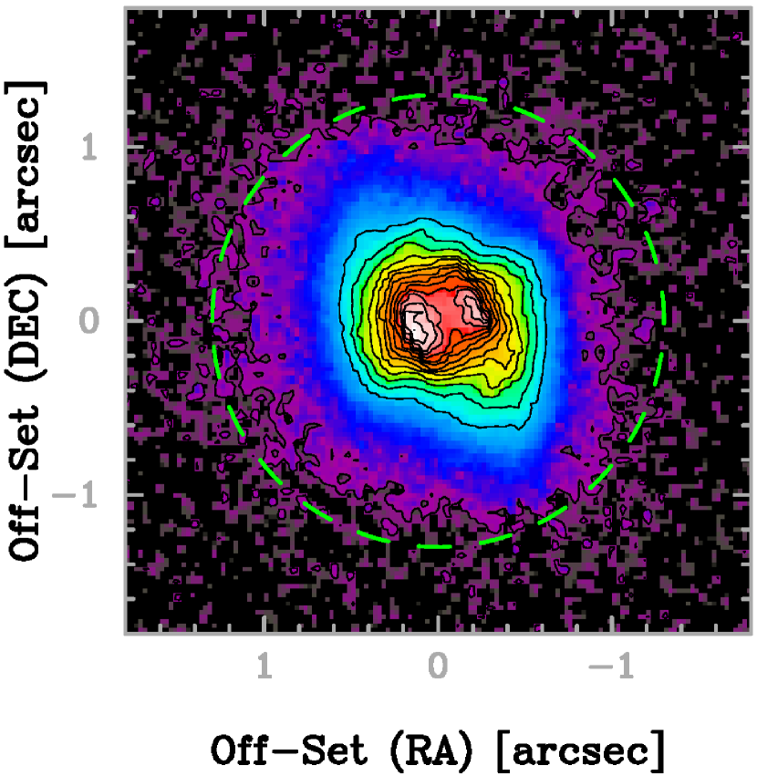
Figure 2: $HST$/WFPC2 F656N (H$\alpha$) image of Wray16-423. The levels of the contour plots are from 3-$\sigma$ above the mean background intensity to the peak intensity of the object. The radius of the green dashed circle is 1.3^′′.

Table 2: Photometry of the HST/WFPC2 images.

Band	$\lambda_{c}$	Portion	$F_{\lambda}$
	(Å)		(erg s-1 cm-2 Å-1)
F547M($V$)	5483.86	CSPN only	(3.75$\pm$0.34)$\times$10-17
		whole nebula	(1.11$\pm$0.04)$\times$10-15
F656N(H$\alpha$)	6563.76	whole nebula	(9.61$\pm$0.15)$\times$10-14

Note – The $V$-band magnitude of the CSPN is 19.98$\pm$0.20, determined from the F547M image.

We reduced the HST/Wide Field Planetary Camera 2 (WFPC2) F656N (H$\alpha$, $\lambda_{\rm c}$=6563.76 Å, $\Delta\lambda$=53.77 Å) and F547M images ($V$-band, $\lambda_{\rm c}$=5483.86 Å, $\Delta\lambda$=205.52 Å) using the MultiDrizzle (Koekemoer et al., 2003) on PYRAF. The data were taken on 2002 July 25 (Prop.ID: 9356, PI: A. Zijlstra). We set the plate scales to a constant 0.025″ pixel^-1. The resultant F656N image is displayed in Figure 2. The Wray16-423 image shows an inner cylindrical structure, surrounded by an elliptical nebula shell that extends radially to $\sim$1.3″, as indicated by the green dashed circle. In the F656N and F547M images, we measured the count rates (cts) within the aperture radius of 1.3″, corresponding to the sum of the CSPN’s and nebula’s cts. We measured average (background) cts in an annulus with inner radius 2.1″ and outer radius 2.4″, centered on the CSPN. Finally, we converted the cts into flux density, using the WFPC2 photometric zero-points in erg s^-1 cm^-2 Å^-1 cts^-1. The results are summarised in Table 2.

To measure the pure H$\alpha$ flux using the F656N flux density, one must remove the contribution from both the local continuum and the [N ii] $\lambda$ 6548 Å. We used the FEROS spectrum to estimate these contributions. Taking into account the F656N filter transmission characteristics, we compared the $F_{\lambda}$(HST,F656N) with the counterpart FEROS spectrum, i.e., $F_{\lambda}$(FEROS,F656N). Finally, we determined the scaling factor $F_{\lambda}$(HST,F656N)/$F_{\lambda}$(FEROS,F656N) = 2.383.

Using this scaled FEROS spectrum, we measured a pure $F$(H$\alpha$) of (4.70$\pm$0.03)$\times$10^-12 erg s^-1 cm^-2 and a pure $F$(H$\beta$) of (1.53$\pm$0.02)$\times$10^-12 erg s^-1 cm^-2. We used the measured pure $F$(H$\beta$) to normalise the flux in the flux density scaled Spitzer/IRS spectrum, as explained in the previous section.

Next, we measured the $V$-band flux density of the CSPN in the F547M image. In the flux density measurements of the CSPN, we need to select the background area more carefully because the CSPN is embedded in a bright nebula and therefore the CSPN magnitude largely depends on the background region adopted. The background cts adopted in the flux density measurement of the whole nebula are not suitable for the flux density measurements of the CSPN. For this reason, we measured cts in four positions near ($\sim$0.2-0.3″ away) the CSPN and used the average cts as the sky background. The measured flux density of the CSPN in the F547M band corresponds to the $V$-band magnitude $m_{V}$ of 19.98$\pm$0.20, which is about 1 magnitude fainter than Zijlstra et al. (2006a, $m_{V}$=18.85$\pm$0.20). The difference would be attributed to the adopted background region; the $m_{V}$ is 18.73$\pm$0.10 when as the background we use the average cts measured in the area of the annulus centered on the PN with inner and outer radii of 2.1″ and 2.4″, respectively.

3 Results

3.1 Reddening correction, line-flux measurements, and radial velocity

Figure 3: (from left to right) The emission line profiles of the [O ii] $\lambda$ 3726.03 Å, H$\gamma$ 4340.46 Å, and [O iii] $\lambda$ 4958.91 Å, from HDS observations. The wavelength is converted into radial velocity with respect to the systemic radial velocity of +133.12 km s^-1. The flux density is normalised to the flux density at the peak.

The measured line fluxes in the obtained spectra were de-reddened using the following formula:

$$I(\lambda)=F(\lambda)\times 10^{c({\rm H}\beta)(1+f(\lambda))},$$ (1)

where $I$($\lambda$) is the de-reddened line-flux, $F$($\lambda$) is the observed line-flux, $f$($\lambda$) is the interstellar extinction function at $\lambda$ computed by the reddening law of Cardelli et al. (1989) with $R_{V}$=3.1, and $c$(H$\beta$) is the reddening coefficient at H$\beta$. For the Spitzer/IRS spectrum, we adopted the reddening law of Fluks et al. (1994).

We measured $c$(H$\beta$) by comparing the observed Balmer line ratios of H$\gamma$ and H$\alpha$ to H$\beta$ with the theoretical ratios of Storey & Hummer (1995) for an electron temperature $T_{\epsilon}$=10⁴ K and electron density $n_{\epsilon}$=10⁴ cm^-3, under the Case B assumption. The H$\alpha$ line in the HDS short-exposure spectrum taken in the 2012 run was affected by cosmic rays. Therefore, we used a $c$(H$\beta$) value of 0.132$\pm$0.035, determined from the $F$(H$\gamma$)/$F$(H$\beta$) ratio. This $c$(H$\beta$) value is in excellent agreement with that in the 2014 HDS run (0.133$\pm$0.063). In the FEROS spectrum, we obtained a $c$(H$\beta$) value of 0.110$\pm$0.022 from the $F$(H$\alpha$)/$F$(H$\beta$) ratio.

We fitted the emission lines in the HDS and FEROS spectra using multiple Gaussian components. Figure 3 shows the emission line profiles of the [O ii] $\lambda$ 3726.03 Å, H$\gamma$ $\lambda$ 4340.46 Å, and [O iii] $\lambda$ 4958.91 Å. We obtained a heliocentric radial velocity of +133.12$\pm$0.28 km s^-1 (RMS of the residuals: 3.17 km s^-1) from the central wavelengths of all the lines detected in the HDS and FEROS spectra. Most line profiles can be fitted by a single Gaussian component, whereas several lines show double peaks or blue-shifted asymmetry, as seen in [O ii] and [O iii].

We list the observed wavelengths and de-reddened relative fluxes of each Gaussian component, indicated by the identification (ID) number in Table 10 of Appendix A, with respect to the de-reddened H$\beta$ flux $I$(H$\beta$) of 100. For lines composed of multiple components, we list the de-reddened relative fluxes of each component, as well as the sum of these components (indicated by ’T’). In the ions showing multiple intensity peaks such as [O ii] $\lambda$3726 Å, one could derive electron temperatures and densities in each Gaussian component. In our data, it would be difficult to accurately derive their ionic abundances relative to the H⁺ in each component because each velocity component of the detected lines are different. Since our aim is to investigate average ionic and elemental abundances in the nebula, we used the integrated fluxes of each Gaussian component. We list the results of the flux measurements for the Spitzer/IRS spectrum in Table 11 of Appendix A, where we adopted the $c$(H$\beta$) of 0.110$\pm$0.022, which is the same value applied for the FEROS spectrum.

3.2 Plasma diagnostics

Figure 4: $n_{\epsilon}$-$T_{\epsilon}$ diagram based on diagnostic CEL ratios. Each curve is labelled with an ID number, listed in Table 3. The thick lines indicate the lines of $T_{\epsilon}$ diagnostic. The dashed lines indicate the diagnostic lines of $n_{\epsilon}$. The $n_{\epsilon}$-$T_{\epsilon}$ curve calculated from the $[$N i$]$ $I$($\lambda$ 5198)/$I$($\lambda$ 5200) is out of the plane, because $n_{\epsilon}$=1010 cm^-3.

Table 3: Plasma diagnostics.

ID	$n_{\epsilon}$ diagnostic	Value	Result
			(cm-3)
(1)	$[$S ii$]$($\lambda$ 6716)/($\lambda$ 6731)	0.60$\pm$0.03	3970$\pm$690
(2)	$[$O ii$]$($\lambda$ 3726)/($\lambda$ 3729)	1.82$\pm$0.13	3540$\pm$790
(3)	$[$S iii$]$($\lambda$ 18.7 $\mu$m)/($\lambda$ 33.5 $\mu$m)	2.30$\pm$0.19	6860$\pm$1060
(4)	$[$O ii$]$($\lambda$ 3726/29)/($\lambda$ 7320/30)	7.42$\pm$0.54	6870$\pm$650
(5)	$[$Cl iii$]$($\lambda$ 5517)/($\lambda$ 5537)	0.69$\pm$0.03	8280$\pm$870
(6)	$[$Ar iv$]$($\lambda$ 4711)/($\lambda$ 4740)	0.68$\pm$0.01	11 320$\pm$540
(7)	$[$Ne iii$]$($\lambda$ 15.6 $\mu$m)/($\lambda$ 36.0 $\mu$m)	15.43$\pm$1.28	23 250$\pm$8230
	$[$N i$]$($\lambda$ 5198)/($\lambda$ 5200)	1.42$\pm$0.12	1010$\pm$260
	Paschen decrement		25 700$\pm$6300
ID	$T_{\epsilon}$ diagnostic	Value	Result
			(K)
(8)	$[$S iii$]$($\lambda$ 9069)/($\lambda$ 18.7 $\mu$m+33.5 $\mu$m)	0.56$\pm$0.05	11 270$\pm$1060
(9)	$[$Ne iii$]$($\lambda$ 3869+$\lambda$ 3967)/($\lambda$ 15.6 $\mu$m)	1.87$\pm$0.12	12 800$\pm$300
(10)	$[$O iii$]$($\lambda$ 4959+$\lambda$ 5007)/($\lambda$ 4363)	106.4$\pm$1.8	12 380$\pm$80
(11)	$[$N ii$]$($\lambda$ 6548+$\lambda$ 6583)/($\lambda$ 5755)	54.4$\pm$2.0	12 090$\pm$230
(12)	$[$Ar iii$]$($\lambda$ 7135+$\lambda$ 7751)/($\lambda$ 5191)	107.8$\pm$5.2	12 000$\pm$250
(13)	$[$Cl iv$]$($\lambda$ 8046)/($\lambda$ 5323)	26.8$\pm$5.7	11 810$\pm$1020
(14)	$[$S ii$]$($\lambda$ 6717+$\lambda$ 6731)/($\lambda$ 4069)	3.81$\pm$0.16	12 760$\pm$810
(15)	$[$S iii$]$($\lambda$ 9069)/($\lambda$ 6312)	5.62$\pm$0.48	12 920$\pm$620
	He i($\lambda$ 7281)/($\lambda$ 5876)	0.066$\pm$0.003	13 600$\pm$1770
	He i($\lambda$ 7281)/($\lambda$ 6678)	0.145$\pm$0.003	11 700$\pm$550
	(Paschen Jump)/(P11)	0.018$\pm$0.002	11 690$\pm$2090

Note – Corrected recombination contribution for $[$O ii$]$ $\lambda\lambda$ 7320/30 Å and $[$O iii$]$ $\lambda$ 4363 Å lines.

In the following line-diagnostics and subsequent ionic element calculations, the adopted transition probabilities, effective collision strengths, and recombination coefficients are the same as those listed in Tables 7 and 11 of Otsuka et al. (2010).

We calculated the electron densities $n_{\epsilon}$ and temperatures $T_{\epsilon}$ using the diagnostic line ratios of RLs and CELs. The results are summarised in Table 3; the second, third, and last columns give the diagnostic lines, their line ratios, and the resulting $n_{\epsilon}$ and $T_{\epsilon}$, respectively. The numbers in the first column indicate the ID number of each curve in the $n_{\epsilon}$-$T_{\epsilon}$ diagram, presented in Figure 4. The thick lines indicate the diagnostic lines for $T_{\epsilon}$, whereas the dashed lines correspond to $n_{\epsilon}$ diagnostics. Below, we explain in detail the $n_{\epsilon}$ and $T_{\epsilon}$ calculations using RLs and CELs.

3.2.1 RL diagnostics

The intensity ratio of a high-order Paschen line P$n$ (where $n$ is the principal quantum number of the upper level) to a lower-order Paschen line is sensitive to the $n_{\epsilon}$, as demonstrated in Fang & Liu (2011). The Paschen decrement can be an $n_{\epsilon}$ indicator for high-density regions. As such, we ran small grid models to estimate $n_{\epsilon}$.

We calculated the electron temperatures derived from He i lines $T_{\epsilon}$(He i) using the two He i line ratios and the emissivities of these He i lines from Benjamin et al. (1999) for the case of $n_{\epsilon}$=10⁴ cm^-3. For He^+,2+ abundance calculations, we adopted the $T_{\epsilon}$(He i)=12 650$\pm$1320 K, which is the average between the values derived from He i $I$($\lambda$ 7281 Å)/$I$($\lambda$ 5876 Å) and He i $I$($\lambda$ 7281 Å)/$I$($\lambda$ 6678 Å).

We calculated the electron temperature derived from the Paschen jump discontinuity $T_{\epsilon}$(PJ) by applying Equation (7) of Fang & Liu (2011):

$$T_{\epsilon}({\rm PJ})=8.72\times\left(1+0.52\frac{\rm He^{+}}{\rm H^{+}}+4.40\frac{\rm He^{2+}}{\rm H^{+}}\right)\cdot\left(\frac{I_{\lambda}({\rm PJ})}{I({\rm P11})}\right)^{-1.77},$$ (2)

where He^+,2+/H⁺ is the ionic He⁺ abundance of 9.63(–2) and He²⁺ abundance of 1.08(–2), respectively, $I_{\lambda}$(PJ) is the strength of the Paschen jump – i.e. the difference in de-reddened flux density between 8169 Å and 8194 Å in erg s^-1 cm^-2 Å^-1, and $I$(P11) is the flux of the H i $\lambda$ 8862 Å in erg s^-1 cm^-2. Because the H i $\lambda$ 8862 Å line is in an order gap, we estimated $I$(P11) using the theoretical ratio of $I$(P11)/$I$(P12)=1.3 in the Case B $T_{\epsilon}$=10⁴ K and $n_{\epsilon}$=10⁴ cm^-3 (Storey & Hummer, 1995). We adopted the $T_{\epsilon}$(PJ) for the RL C^2+,3+,4+ and O²⁺ abundance calculations.

3.2.2 CEL diagnostics

We derived the CEL $T_{\epsilon}$ and $n_{\epsilon}$ by solving for level populations using a multi-level atomic model ($\geq$5), resulting in eight calculated $n_{\epsilon}$, including $n_{\epsilon}$([N i]), as well as eight $T_{\epsilon}$.

For the [O ii] $\lambda\lambda$ 7320/30 Å and [O iii] $\lambda$ 4363 Å lines, we subtracted the recombination contamination from the O²⁺ and O³⁺ lines using Equations (3) and (4), originally given by Liu et al. (2000),

$$\frac{I_{R}(\rm[O\,{\sc II}]\,\lambda\lambda\,7320/30)}{I(\rm H\beta)}=9.36\left(\frac{T_{\epsilon}}{10^{4}}\right)^{0.44}\times\frac{\rm O^{2+}}{\rm H^{+}},$$ (3)

$$\frac{I_{R}(\rm[O\,{\sc III}]\,\lambda\,4363)}{I(\rm H\beta)}=12.4\left(\frac{T_{\epsilon}}{10^{4}}\right)^{0.59}\times\frac{\rm O^{3+}}{\rm H^{+}}.$$ (4)

In the $I_{R}$([O ii] $\lambda\lambda$ 7320/30) calculation, we adopted the $T_{\epsilon}$(PJ) and recombination O²⁺ abundances (3.12$\times$10^-4, see Section 3.3.2). For the $I_{R}$([O iii] $\lambda$ 4363) calculation, we used the O³⁺ abundance derived from the fine-structure [O iv] $\lambda$ 25.89 $\mu$m line (6.93$\times$10^-6, See section 3.3.1) and $T_{\epsilon}$([Ne iii]). $I_{R}$([O ii] $\lambda\lambda$ 7320/30) and $I_{R}$(([O iii] $\lambda$ 4363) were 0.86 and 0.01, respectively.

Walsh et al. (1997) reported a single $T_{\epsilon}$ of 12 400$\pm$400 K and $n_{\epsilon}$ of 6000$\pm$1500 cm^-3. In the present study, we first calculated all $n_{\epsilon}$(CEL)s under their derived value $T_{\epsilon}$=12 400 K, except for $n_{\epsilon}$([N i]), where we assumed a $T_{\epsilon}$ of 10 000 K because the effective collisional strengths of the Mg⁰ is available at $T_{\epsilon}$=10 000 K (See Section 3.3.1 for details). The $T_{\epsilon}$=10 000 K would be a good choice for estimates of neutral atoms such as N⁰ and O⁰ even in high-excitation PNe such as BoBn1 (Otsuka et al., 2010). We derived $T_{\epsilon}$([Ne iii]) using $n_{\epsilon}$([Ar iv]) because the ionisation potentials (IPs) of both ions are similar. We derived $T_{\epsilon}$([O iii]) and $T_{\epsilon}$([Cl iv]) under the average $n_{\epsilon}$ among $n_{\epsilon}$([Ar iv],[Cl iii],[S iii]); the IPs of the [O iii] and [Cl iv] are approximately median between $n_{\epsilon}$(C iii&[S iii],[Ar iv]) or slightly larger than these ions. We calculated $T_{\epsilon}$([Ar iii]) and two $T_{\epsilon}$([S iii]) under the average $n_{\epsilon}$ between $n_{\epsilon}$([Cl iii],[S iii]). $T_{\epsilon}$([N ii]) and $T_{\epsilon}$([S ii]) were calculated under the average $n_{\epsilon}$ among the two $n_{\epsilon}$([O ii]) and $n_{\epsilon}$([S ii]).

3.3 Ionic abundances

3.3.1 CEL ionic abundances

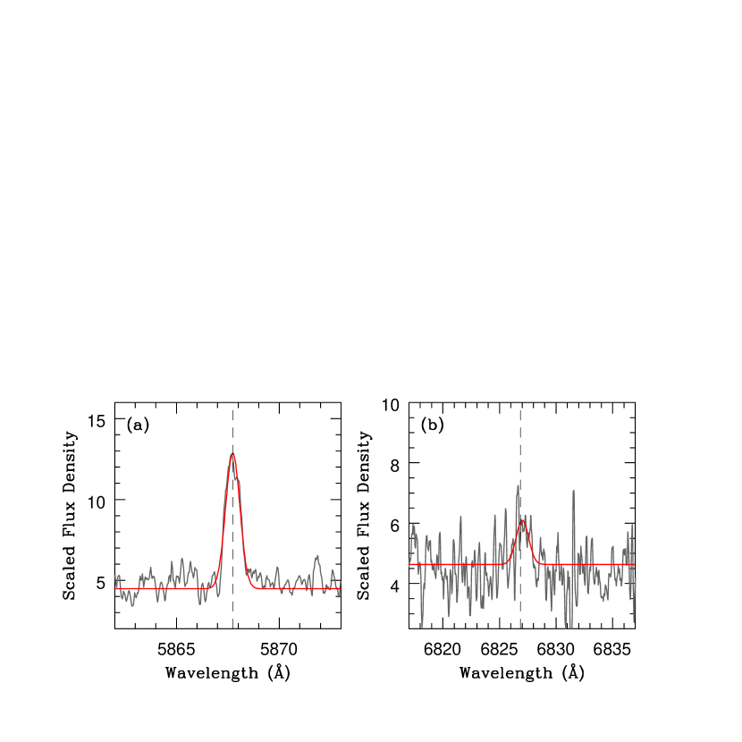
Figure 5: The line profiles of the $[$Kr iv$]$ $\lambda$ 5867.74  Å (left panel) and the $[$Kr iii$]$ $\lambda$ 6826.85 Å (right panel). The grey lines are the observed spectra at the rest wavelength, which is shifted by the systemic heliocentric radial velocity (+133.12 km s^-1). The sky emission lines were removed out as much as possible. The red lines are the results of Gaussian fitting. The laboratory wavelengths of these lines are indicated by the dashed lines.

We obtained 21 ionic abundances using CELs, as listed in Table 12 of Appendix B. We carefully determined the adopted $T_{\epsilon}$ and $n_{\epsilon}$ pairs for the calculations of each ion using the $n_{\epsilon}$-$T_{\epsilon}$ diagram. The adopted $T_{\epsilon}$ and $n_{\epsilon}$ values for each ion are listed in the fourth and fifth columns of Table 12, respectively. For the Mg⁰ abundance calculation, we adopted the effective collision strengths installed in the three-dimensional Monte Carlo photoionisation code Moccasin (Ercolano et al., 2003) and the transition probabilities of Mendoza (1983). Because the effective collision strengths of Mg⁰ are only available at the case of $T_{\epsilon}$=10⁴ K, we adopted this temperature. $T_{\epsilon}$=10⁴ K and $n_{\epsilon}$([N i]) were used for the N⁰ and Mg⁰ calculations. The ionic abundances were calculated by solving the statistical equilibrium equations for more than five levels, given the adopted $T_{\epsilon}$ and $n_{\epsilon}$, except for Ne⁺, where we calculated its abundance using the two-energy level model. The last column contains the resulting ionic abundances relative to the H⁺, X^m+/H⁺, and their 1-$\sigma$ errors, which include errors from line intensities, $T_{\epsilon}$, and $n_{\epsilon}$, but does not consider the accuracy of the atomic data. In the O⁺ and O²⁺ abundance calculations, we corrected the line intensities of the [O ii] $\lambda\lambda$ 7320/30 Å and [O iii] $\lambda$ 4363 Å, respectively. In the last line of each ion’s line series, the adopted ionic abundance and its error are indicated in boldface. These values are estimated from the weighted mean of the line intensity.

As presented in Table 12, the calculated abundances of each ion using different transition lines (i.e., fine-structure, nebular, auroral, and trans-auroral lines) are well consistent (within the error), indicating proper selection of the adopted $T_{\epsilon}$ and $n_{\epsilon}$ pairs for each ion and accurate measurement of the flux.

We report the first detection of the [Kr iv] $\lambda$ 5867.74 Å and [Kr iii] $\lambda$ 6826.85 Å in Wray16-423. The line profiles are presented in Figure 5. The sky emission lines between $\sim$6820 and 6830 Å were subtracted as much as possible. Because there are no candidate lines within 0.18-0.20 Å from the measured central wavelengths of the above lines (5867.74 Å and 6827.02 Å at rest), we concluded that the lines corresponded to krypton. Krypton lines have been observed in the Sgr dSph PNe, specifically, BoBn1 (Otsuka et al., 2010) and Hen2-436 (Otsuka et al., 2011). The Kr²⁺ abundance in Wray16-423 is comparable to that in Hen2-436, which shows the same metallicity.

3.3.2 RL ionic abundances

We list the RL ionic abundances in Table 13 of Appendix B. To the best of our knowledge, RL C^3+,4+ and O²⁺ for Wray16-423 are reported for the first time. Because we detected C ii,iii,iv and O ii lines, we were able to calculate the elemental C/O ratio using the same type of emission lines.

In the abundance calculations, we adopted the Case B assumption for the lines from levels that have the same spin as the ground state, but the Case A assumption for lines of other multiplicities. In the last line of each ion’s line series, we present the adopted final ionic abundance and its 1-$\sigma$ error estimated from the line intensity-weighted mean, indicated by boldface. Because the RLs are $n_{\epsilon}$-insensitive under $\lesssim$10⁸ cm^-3, we evaluated the recombination coefficients (provided as a polynomial function of $T_{\epsilon}$) at a constant $n_{\epsilon}$=10⁴ cm^-3 for all lines.

In the He⁺ abundance calculations, using He i $\lambda$ 4471 Å and He i $\lambda$ 5876 Å lines, we assumed Case A conditions and adopted the recombination coefficients of Pequignot et al. (1991). We subtracted the contribution to these lines by collisional excitation from the He⁰ $2s$³$S$ level, using the formulae given by Kingdon & Ferland (1995).

We detected the different multiplet O ii lines. Because the electron density in the O²⁺ emitting region is $\gtrsim$10⁴ cm^-3 from our plasma diagnostics, the upper levels of the transitions in the V1 O ii line would be in local thermal equilibrium (LTE). Therefore, we did not correct the V1 O ii line intensities. To calculate the O²⁺ abundances, we excluded the V1 O ii $\lambda$ 4641.81/4651.33/4673.73 Å and V2 O ii $\lambda$ 4325.76 Å lines. The first two V1 lines are likely contaminated with N iii $\lambda$ 4641.85 Å and C iii $\lambda$ 4651.47 Å, respectively. The O²⁺ abundance derived from the O ii $\lambda$ 4673.73 Å line is larger than that from other V1 lines. The last V2 line is likely contaminated with C ii $\lambda$ 4325.83 Å.

The RL O²⁺ abundance is larger by a factor of 1.64$\pm$0.43 larger than the O²⁺ CEL. According to Liu (2006), the O²⁺ discrepancy factor in Wray16-423 would be a lower limit. As proposed for the halo H4-1 (O²⁺ discrepancy factor=1.75$\pm$0.36; Otsuka & Tajitsu, 2013), we speculate that the O²⁺ discrepancy in Wray16-423 could be explained because the estimated CEL O²⁺ abundance could be increased by $\sim$0.2 dex or less if we include temperature fluctuations, which is originally proposed by Peimbert (1967). Since the O²⁺ discrepancy factor is already low, we do not discuss further in the paper.

3.4 Elemental abundances

Table 4: Elemental abundances from CELs and RLs.

(1)	(2)	(3)	(4)	(5)	(6)	(7)	(8)	(9)	(10)
X	Types of	X/H	$\log_{10}$(X/H)	[X/H]	$\log_{10}$(X⊙/H)a	ICF(X)	$\log_{10}$(X/H)	$\log_{10}$(X/H)	$\log_{10}$(X/H)
	Emissions		+12		+12		+12 (Ref.1)	+12 (Ref.2)	+12 (Ref.3)
He	RL	1.06(–1)$\pm$9.56(–3)	11.02$\pm$0.04	+0.09$\pm$0.04	10.93$\pm$0.01	1.00	11.03$\pm$0.01	11.03$\pm$0.02	11.09$\pm$0.05
C	RL	8.29(–4)$\pm$1.57(–4)	8.92$\pm$0.08	+0.53$\pm$0.09	8.39$\pm$0.04	1.00	8.86$\pm$0.06		9.08$\pm$0.35
N	CEL	4.94(–5)$\pm$5.04(–6)	7.69$\pm$0.04	–0.14$\pm$0.07	7.83$\pm$0.05	24.81$\pm$2.12	7.68$\pm$0.05	7.62$\pm$0.10	7.38$\pm$0.22
O	CEL	2.06(–4)$\pm$4.10(–6)	8.31$\pm$0.01	–0.38$\pm$0.05	8.69$\pm$0.05	1.00	8.33$\pm$0.02	8.31$\pm$0.07	8.35$\pm$0.03
	RL	3.37(–4)$\pm$8.90(–5)	8.53$\pm$0.11	–0.16$\pm$0.13	8.69$\pm$0.05	1.08$\pm$0.03	$\cdots$	$\cdots$	9.56$\pm$0.11
Ne	CEL	4.09(–5)$\pm$2.93(–6)	7.61$\pm$0.03	–0.26$\pm$0.10	7.87$\pm$0.10	1.00	7.55$\pm$0.03	7.50$\pm$0.08	7.62$\pm$0.05
S	CEL	2.51(–6)$\pm$1.58(–7)	6.40$\pm$0.03	–0.79$\pm$0.05	7.19$\pm$0.04	1.00	6.67$\pm$0.04	6.48$\pm$0.08	6.83$\pm$0.08
Cl	CEL	5.42(–8)$\pm$5.66(–9)	4.74$\pm$0.05	–0.77$\pm$0.30	5.50$\pm$0.30	1.00	4.89$\pm$0.18	$\cdots$	4.86$\pm$0.09
Ar	CEL	1.00(–6)$\pm$3.85(–8)	6.00$\pm$0.02	–0.55$\pm$0.08	6.55$\pm$0.08	1.00	5.95$\pm$0.07	5.88$\pm$0.08	5.95$\pm$0.32
K	CEL	2.02(–8)$\pm$2.30(–9)	4.31$\pm$0.05	–0.80$\pm$0.07	5.11$\pm$0.05	3.06$\pm$0.23	4.65$\pm$0.22	$\cdots$	$\cdots$
Fe	CEL	3.62(–7)$\pm$5.62(–8)	5.56$\pm$0.07	–1.91$\pm$0.07	7.47$\pm$0.03	23.81$\pm$2.12	$\cdots$	$\cdots$	5.73$\pm$0.20
Kr	CEL	3.52(–9)$\pm$4.88(–10)	3.55$\pm$0.06	+0.27$\pm$0.10	3.28$\pm$0.08	1.00	$\cdots$	$\cdots$	3.62$\pm$0.13

References (1) Zijlstra et al. (2006a), Dudziak et al. (2000), (2) (2) Walsh et al. (1997) for Wray16-423; (3) Otsuka et al. (2011) for Hen2-436.
^aAsplund et al. (2009) for N and Cl, and Lodders (2003) for the other elements.

The elemental abundances of the nebula are listed in Table 4. The types of emission lines used for the abundance estimations are specified in the second column. The fifth column lists the number densities relative to the solar value, where [X/H] corresponds to $\log_{10}$(X/H)-$\log_{10}$(X/H)_⊙.

To estimate elemental abundances using only the observed ionic abundances, we introduced an ionisation correction factor, ICF(X), based on the ionisation potential. The adopted ICF(X) for each element is listed in Table 14 of Appendix B, and the value is listed in the seventh column of Table 4. We calculated the adopted ICF(Kr) using Equation (5) of Sterling et al. (2007), based on photoionisation models.

In the eighth column of Table 4, we list the elemental abundances of Wray16-423 compiled by Zijlstra et al. (2006a), originally calculated using the photoionisation model of Dudziak et al. (2000) based on the analysis of optical spectra by Walsh et al. (1997). The ninth column is the result of Walsh et al. (1997). In general, our calculated abundances, except for S and K, are in excellent agreement with prior results. Walsh et al. (1997) reported a C²⁺/O²⁺ ratio of 3.4$\pm$1.2, derived from C ii and [O iii] lines (C²⁺(RL)/O²⁺(CEL)=2.48$\pm$0.74 in the present work). Assuming that C(RL)/O(CEL) $\simeq$ C²⁺/O²⁺, their C abundance would be 5.99(–4)$\pm$2.17(–4), which corresponds to 8.78$\pm$0.16 dex. The differences of the S and K abundances between Zijlstra et al. (2006a) and ours might be caused by adoption of different $T_{\epsilon}$ for these ionic abundances and overestimate of the S³⁺ abundance. The [S iv] lines are not seen in optical but in mid-infrared wavelength. Their photoionisation without dust grains would affect the nebula’s density and temperature structure and the fraction of each element’s ion.

The RL C/O ratio of 2.46$\pm$0.80 indicates that Wray16-423 is presumably a C-rich PN. Elemental RL and CEL O abundances seem to follow the trend; as shown in Liu (2006), Wang & Liu (2007), and Delgado-Inglada & Rodríguez (2014), the RL C/O ratio seems to be consistent with the CEL C/O ratio within errors (.i.e., the RL C/O $\simeq$ the CEL C/O), except for several objects. If this is also the case for Wray16-423, the CEL C abundance would be 8.70$\pm$0.14, where the upper value is consistent with the lower value of the RL C abundance.

The noble gas Ar is not easily tied up in dust grains, and is also not synthesised in low-intermediate mass stars. Therefore, Ar can be used as a metallicity indicator of the progenitor star. The [Ar/H] abundance is consistent with that in Hen2-436 (–0.60$\pm$0.33, Otsuka et al., 2011). Like for Hen2-436, [Fe/H] is significantly lower than [Ar/H]. Because [Fe iii] intensities are comparable to BoBn1 (Otsuka et al., 2011) and their Fe²⁺ abundances in Wray16-423 and BoBn1 are consistent, the small Fe abundance in Wray16-423 cannot be attributed to inaccuracies in Fe²⁺ atomic data or the selection of $T_{\epsilon}$ for their ionic abundances. Thus, a large fraction of Fe atoms would exist as dust grains.

An important contribution of our work is the detection of the light $s$-process element Kr and calculation of its abundance. This required verification of whether or not the Kr abundance value for Wray16-423 is reasonable. Sterling & Dinerstein (2008) examined the relationship between the [Kr/O] and C/O ratio, based on their $Ks$-band spectroscopic survey for Galactic PNe, from which the following relationship was obtained:

$${\rm[Kr/O]=(0.38\pm 0.10)+(0.79\pm 0.29)\cdot\log_{10}(C/O)}.$$ (5)

By substituting the observed RL $\log_{10}$(C/O) ratio, we obtained a predicted [Kr/O] value of +0.69$\pm$0.42, which is in good agreement with the observed [Kr/O] of +0.65$\pm$0.11 from Kr and O CELs. The authors also showed the light $s$-enhancement ([ls/Fe], ls: Sr, Y, and Zr) versus the C/O ratio among AGB stars and CH sub-giants:

$${\rm[ls/Fe]=(0.89\pm 0.06)+(1.47\pm 0.18)\cdot\log_{10}(C/O)}.$$ (6)

As described above, the calculated Fe abundance in Wray16-423 may not accurately reflect the correct metallicity. Given that [Fe/H] is equal to [Ar/H], the [ls/Ar]=[Kr/Ar] is moderately enhanced, +0.82$\pm$0.13. This value is slightly smaller than the predicted [ls/Fe] of 1.46$\pm$0.44 from Equation (6), although it depends on the adopted metallicity. There are a few results on the $s$-process in carbon stars in the Sgr dSph. For example, de Laverny et al. (2006) reported $s$-process enhancements in two C-rich stars (C/O=1.05-1.18). The respective [ls/Fe]s in IGI95-C1 ([M/H]=–0.8, [ls/M]=+0.6) and IGI95-C3 ([M/H]=–0.5, [ls/M]=+1.0) are comparable to that in Wray16-423. In comparison with previous studies of PNe and AGB stars, we concluded that the Kr abundance value obtained for Wray16-423 is reasonable.

In the last column of Table 4, we list the elemental abundance of Hen2-436 by Otsuka et al. (2011); the abundances obtained in the present study, with the exception of N, are close to those for Hen2-436. The O and Ar abundances indicate that both PN progenitors would form under a similar evolutionary stage of the Sgr dSph. Dudziak et al. (2000) pointed out that the nearly identical abundance patterns for these two Sgr dSph PNe provide evidence that the progenitors formed in a single starburst event ($\sim$5 Gyrs ago, Zijlstra et al., 2006a) within a well mixed ISM. The age-metallicity relationship for the Sgr dSph globular cluster candidates by Law & Majewski (2010) indicates that the [Fe/H]$\sim$–0.6 corresponds to $\sim$8 Gyrs ago. Layden & Sarajedini (2000) reported that the Sgr dSph field is composed of several different populations; the [Fe/H]=–0.7$\pm$0.2 population is 5$\pm$1 Gyrs old and the [Fe/H]=–0.4$\pm$0.3 population is 0.5-3 Gyrs old. Although the exact [Fe/H] abundances in Wray16-423 and Hen2-436 are unknown, the progenitor stars of Wray16-423 and Hen2-436 most likely formed 0.5-6 Gyrs ago.

3.5 [WC] type central star

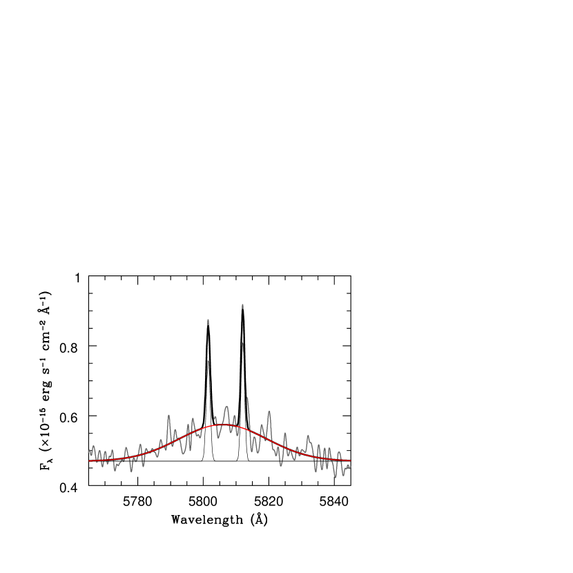
Figure 6: The observed profile of the C iv $\lambda\lambda$ 5801/12 Å band indicated by the grey line. The observed wavelength is corrected by the heliocentric radial velocity of +133.12 km s^-1. An interesting feature (perhaps originating from a stellar wind), is indicated by the red line.

In Figure 6, we present the profile of the C iv $\lambda\lambda$ 5801/12 Å band composed of narrow nebular C iv $\lambda\lambda$ 5801/12 Å lines and a weak broad wing component (perhaps originating from a stellar wind). We fitted the band profile by three Gaussian components: in Figure 6, the thin black lines are the components of the nebular C iv $\lambda\lambda$ 5801/12 Å, the red line indicates our interesting broad component, and the thick black line is the sum of these three. The FWHMs of the C iv $\lambda\lambda$ 5801/5812 Å lines are 0.75$\pm$0.04 and 0.83$\pm$0.05 Å and that of the broad component (centered at 5805.96 Å in the rest frame) is 32.12$\pm$2.15 Å, where its FWHM expansion velocity is 1660$\pm$110 km s^-1. The C iv $\lambda\lambda$ 5801/12 Å band profile in Wray16-423 is similar to the Sgr dSph PN StWr2-21; Kniazev et al. (2008) de-convolved the C iv $\lambda\lambda$ 5801/12 Å into three components, which included a broad component having a FWHM of 42.3$\pm$3 Å. Although the nebular C iv $\lambda\lambda$ 5801/5812 Å lines seem to be completely embedded in the broad component in Hen2-436, the FWHM of the C iv $\lambda\lambda$ 5801/12 Å band is 32.8$\pm$0.2 Å, measured from the same ESO VLT/FEROS2 spectra used in Otsuka et al. (2011), and consistent with the findings of Walsh et al. (1997, 31.1 Å). We did not detect any other broad components, such as O vi $\lambda\lambda$ 3811/34 Å.

A consensus has not been reached regarding the classification of the CSPN of Wray16-423. Walsh et al. (1997) classified it as a [WC8] or a weak emission line star (WELS), on the basis of the strengths of the C iii $\lambda$ 4650 Å (FWHM=9.9 Å) and C iv $\lambda\lambda$5801/12 Å (FWHM=14.7 Å) bands, using low-dispersion spectra ($R$ could be $\sim$1200 around 5800 Å); the broad component under the nebular C iv $\lambda\lambda$ 5801/5812 Å lines was not detected. The broad component of the C iii and C iv complex centered around 4650 Å, originating from the stellar winds, is not clearly seen in our HDS and FEROS spectra. There is no broad component in the C ii $\lambda$4267 Å, too.

Taking into account that their estimated CSPN temperature (85 000 K) is hot for a [WC8] PNe, Walsh et al. (1997) concluded that Wray16-423 could fall into WELS. Acker et al. (2002) analysed 42 emission line nuclei of PNe, and reported that the [WC4] CSPNe show the highest temperatures among the [WC] class (54 950-91 200 K). The determination of CSPN temperatures can be difficult, as pointed out by Acker et al. (2002), which may explain why the CSPN temperatures of the [WC] class PNe have a relatively wide range. Even after the CSPN temperature was corrected up to 107 000 K by photoionisation models based on the low-dispersion spectra of Walsh et al. (1997), Gesicki & Zijlstra (2003) and Zijlstra et al. (2006a) supported the conclusion by Walsh et al. (1997).

According to the classification of Acker et al. (2002), the broad FWHM of the stellar C iv component suggests that the CSPN of Wray16-423 may be a [WC4]-type central star.

3.6 PAHs and dust features

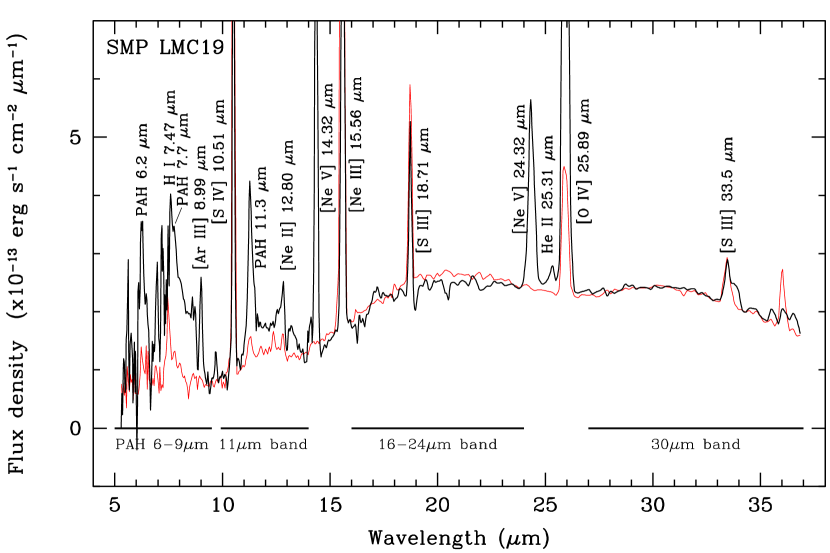
Figure 7: Spitzer/IRS spectrum of SMP LMC19 in the LMC. The intensity-scaled spectrum of Wray16-423 is indicated by the red line. The scaling factor is 2.98, for adjustment to the 16-36 $\mu$m flux density of LMC19.

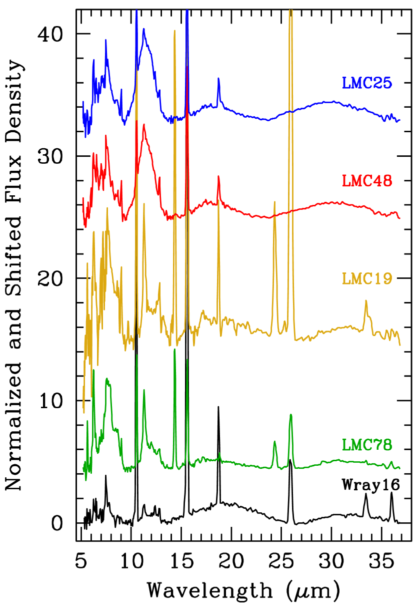
Figure 8: Spitzer/IRS spectra of SMP LMC25, 48, 19, and 78 and Wray16-423 (Wray16). The local continuum was subtracted by fifth-order spline-function fitting. Flux densities are normalised and shifted to emphasise the 16-24 and 30 $\mu$m features.

Wray16-423 shows PAH bands and dust features, specifically, 6-9 $\mu$m and 10-14 $\mu$m PAH bands and broad 11 $\mu$m, 16-24 $\mu$m, and 30 $\mu$m features. These PAH bands and these dust features have been found in C-rich MC PNe (Stanghellini et al., 2007; Bernard-Salas et al., 2009; García-Hernández et al., 2012; Matsuura et al., 2014; Sloan et al., 2014). Bernard-Salas et al. (2009) reported broad 11 $\mu$m, 16-24 $\mu$m, and 30 $\mu$m features in 8 C-rich MC PNe. Because the typical LMC metallicity is close to that of Wray16-423, LMC PNe provide a good comparison in terms of dust production in a metal-deficient environment. Therefore, we looked at the LMC PN sample to compare the mid-IR spectrum of Wray16-423 with those of selected LMC PNe.

Accordingly, we found that SMP LMC19, 25, 48, and 78 exhibit broad 11/16-24/30 $\mu$m features, comparable to the dust feature strengths measured in Wray16-423. Among them, the mid-IR spectrum of LMC19 is most similar to that of Wray16-423 (Fig. 7); the strengths of the broad 16-24 $\mu$m and 30 $\mu$m features and the global $\sim$5-37 $\mu$m SED are similar as well.

For a more detailed look at these PAH and broad dust features, we subtracted the expected local dust continuum, determined by fifth-order spline-function fitting. The resultant spectra are displayed in Figure 8. The flux densities are scaled and shifted to emphasise broad 16-24 $\mu$m and 30 $\mu$m features.

In the following sections, we describe the 6-9 $\mu$m and 10-14 $\mu$m PAH bands, the broad 11 $\mu$m, 16-24 $\mu$m, and 30 $\mu$m band features in Wray16-423, and LMC19, 25, 48, and 78. Dust and gas mass estimates for these LMC PNe will be discussed in a future study.

3.6.1 The 6-9 $\mu$m PAH band

The classification of the 6-9 $\mu$m PAH band is based on the positions of 6.2, 7.7, and 8.6 $\mu$m features at the intensity peaks. According to Peeters et al. (2002) and Matsuura et al. (2014), the 6-9 $\mu$m PAH profiles have peak positions near 6.22-6.3 $\mu$m, 7.6-8.22 $\mu$m, and $\gtrsim$8.6  $\mu$m. Our classifications are summarised in Table 15 of Appendix C. From the overview of Peeters et al. (2002), both the 6.2 and 7.7 $\mu$m PAHs in Wray16-423 are Class $\mathcal{B}$, with corresponding peaks at 6.24$\pm$0.01 $\mu$m, and 7.78$\pm$0.04 $\mu$m, respectively. The 6.2 and 7.7 $\mu$m PAHs in our comparison LMC PNe fall into Classes $\mathcal{B}$ and $\mathcal{A}$, respectively. The 8.6 $\mu$m PAH in Wray16-423 could not be resolved, due to a low signal. The 8.6 $\mu$m PAHs in LMC PNe are classified as Class $\mathcal{B}$.

3.6.2 The 10-14 $\mu$m PAH band and the broad 11 $\mu$m feature

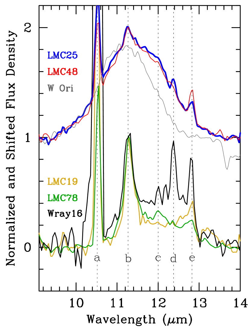
Figure 9: The 9.5-13.5 $\mu$m emission complex showing the 10-14 $\mu$m PAH bands and the broad 11 $\mu$m feature. The vertical dashed lines mark the positions of (a) [S iv] $\lambda$10.51 $\mu$m, (b) 11.3 $\mu$m PAH, (c) 12 $\mu$m PAH, (d) H i $\lambda$ 12.38 $\mu$m, and (e) the 12.7 $\mu$m PAH + [Ne ii] $\lambda$ 12.80 $\mu$m complex. The grey line shows an ISO/SWS spectrum of the Galactic C-rich AGB star W Ori, with the 11 $\mu$m SiC feature.

Figure 9 shows the 10-14 $\mu$m PAH bands complex and the broad 11 $\mu$m feature. The flux densities are normalised with respect to the 11.3- $\mu$m PAH emission peak. The positions of the PAHs and the atomic gas emission lines are shown as vertical dashed lines with the lowercase letters a-e.

In the study on PAHs in LMC post-AGB stars, Matsuura et al. (2014) classified the 10-14 $\mu$m PAH feature into four types: $\alpha$, $\beta$, $\gamma$, and $\delta$, depending on the peak wavelengths and the shapes of the sub-features. The Class $\alpha$ (including the broad 11 $\mu$m feature) shows a sharp feature at 11.3 $\mu$m, a well-isolated feature at 12.7 $\mu$m, and a very weak feature at 12 $\mu$m. The 11.3 $\mu$m PAH emission in Class $\alpha$ is the strongest among the three features. The respective features would be from the solo (11.3 $\mu$m PAH), duo (12 $\mu$m PAH), and trio (12.7 $\mu$m PAH) out-of-plane C-H bending mode of PAH (Sloan et al., 2014). We classify the 10-14 $\mu$m features in Wray16-423, LMC19, and LMC78 as Class $\alpha$. The flux density for these three PNe reaches its maximum in this range at the peak of the 11.3 $\mu$m PAH emission (central wavelengths: 11.28, 11.30, and 11.29 $\mu$m, respectively); 12 $\mu$m PAHs are also observed in all three. The 12.7 $\mu$m PAHs are observed in LMC19 and 78, while the presence of this PAH in Wray16-423 seems to be merged with [Ne ii] $\lambda$ 12.80 $\mu$m.

LMC25 and 48 are characterised as Class $\delta$, by the broad feature extending from 10 to 14 $\mu$m with the 11.3 $\mu$m PAH on the top (Matsuura et al., 2014). Class $\delta$ spectra are quite different from Class $\alpha$ spectra, in terms of the underlying broad 11 $\mu$m feature and its central position. We fitted Gaussians to the PAH and atomic gas emission lines, and subtracted the fits from the spectra. We then fitted the broad 11 $\mu$m feature in the residual spectra was fitted using a single Gaussian component to determine their central wavelengths $\lambda_{c}$ and FWHMs (Table 15). The average peak position and FWHM of the broad feature are 11.92$\pm$0.05 $\mu$m and 1.74$\pm$0.11 $\mu$m, respectively, for Class $\alpha$, while those in Class $\delta$ are 11.46$\pm$0.01 $\mu$m and 1.86$\pm$0.03 $\mu$m, respectively.

Matsuura et al. (2014) argued that the broad 11 $\mu$m feature characteristic to Class $\delta$ should be ascribed to silicon carbide (SiC). They used fits for the 10-14 $\mu$m spectra of three post-AGB stars using the NASA/Ames PAH IR-spectral database (Boersma et al., 2014; Bauschlicher et al., 2010) and the ISO/SWS spectrum of the C-rich AGB star W Ori as the SiC template (see also Fig. 9). Sloan et al. (2014) analyzed the broad 11 $\mu$m features and associated PAHs in LMC and SMC post AGB stars. They call the band profiles similar to LMC25 and LMC48 “Big-11”. They demonstrated that this Big-11 is composed of SiC and PAH, and they concluded that the Big-11 feature is due primarily to SiC (88 $\%$ of the total flux). Otsuka et al. (2015) argued that the broad 11 $\mu$m feature in W Ori could be reproduced using the absorption efficiency $Q_{\lambda}$ of a spherical $\alpha$-SiC grain. Assuming that SiC grains greatly contribute to the 10-14 $\mu$m feature of Class $\delta$, the wider FWHM in Class $\delta$ compared with Class $\alpha$ would then be due to the contribution from the 12 and 12.7 $\mu$m PAHs.

3.6.3 The broad 16-24 $\mu$m feature

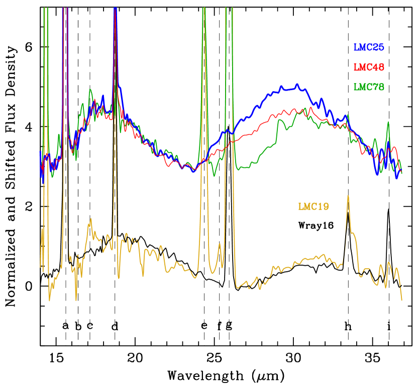
Figure 10: The 14-37.5 $\mu$m continuum subtracted spectra, showing the broad 16-24 $\mu$m and 30 $\mu$m features. The vertical dashed lines mark the positions of (a) [Ne iii] $\lambda$ 15.56 $\mu$m, (b) and (c) 16.4 $\mu$m PAH and 15-18 $\mu$m plateau (possible), (d) [S iii] $\lambda$ 18.71 $\mu$m, (e) [Ne iv] $\lambda$ 24.32 $\mu$m, (f) He ii $\lambda$ 25.31 $\mu$m, (g) [O iv] $\lambda$ 25.89 $\mu$m, (h) [S iii] $\lambda$ 33.50 $\mu$m, and (i) [Ne iii] $\lambda$ 36.01 $\mu$m.

Figure 11: The plot between the 6-9 $\mu$m PAH and the broad 16-24 $\mu$m feature strengths.

Broad 16-24 $\mu$m and 30 $\mu$m features are presented in Fig. 10. Bernard-Salas et al. (2009) and García-Hernández et al. (2012) reported the detection of this feature in MC PNe. Matsuura et al. (2014) detected this feature in the LMC post-AGB star IRAS0588-6944. In our galaxy, a broad 16-24 $\mu$m feature has been found in PNe M1-11 (Otsuka et al., 2013), K3-17, M2-43 (Hony et al., 2002b), and the proto-PN IRAS01005+7910 (Zhang et al., 2010).

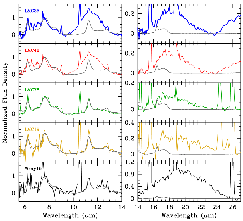
Figure 17: (left panels) The 5.5-14 $\mu$m continuum subtracted spectra, showing the 6-9 $\mu$m and 10-14 $\mu$m PAH bands and the broad 11 $\mu$m feature. Spitzer/IRS continuum subtracted spectrum of the Galactic PN K3-60, indicated by the grey line in each panel, is presented as a template for the 16.4 $\mu$m PAH and 15-18 $\mu$m plateau. We convolved the SH and LH spectra with a Gaussian kernel for the SH and LH module spectra of K3-60 to smooth its spectral resolving power down to those of the SL and LL spectra, respectively. After that, we subtracted the local continuum and gas-emission lines from this spectrum, and then normalised to the intensity peak of the 7.7 $\mu$m PAH band. (right panels) The 14-27 $\mu$m continuum subtracted spectra, showing the broad 16-24 $\mu$m feature. The spectrum of K3-60, indicated by the grey line, is superimposed on each spectrum of the sample PNe. The dashed lines show the wavelength range of the 15-18 $\mu$m plateau + 16.4 $\mu$m PAH.

The 16-24 $\mu$m feature is narrower in LMC25, 48, 78 (See Table 15); this could be due to the contribution of the blue wing of the 30 $\mu$m feature. The band profiles in LMC25, 48, and 78 are slightly asymmetric; the ${\lambda}_{c}$s of the 16-24 $\mu$m feature in these three are blue-shifted, compared with those of Wray16-423 and LMC19. The asymmetric profile could be due to a small plateau superposed on the broad 16-24 $\mu$m around 15-18 $\mu$m. The 15-18 $\mu$m plateau seems to be possibly in LMC19 ($\lambda_{c}$$\sim$17.10 $\mu$m), but its presence is unclear in Wray16-423. In Figure 17 of Appendix C, we compare our sample PNe with the Galactic PN K3-60 (AORKEY: 19903744, PI: H. Dinnerstein, indicated by the grey lines). We use the K3-60 spectrum to explain the position and width of the 15-18 $\mu$m plateau, as an example. K3-60 shows the 15-18 $\mu$m plateau but no broad 16-24 $\mu$m feature. The 6-9 and 10-14 $\mu$m PAH band profiles in K3-60 are well matched to those in LMC78, 19, and Wray16-423. The complex of the 15-18 $\mu$m plateau and the 16.4 $\mu$m PAH also contribute to the broad 16-24 $\mu$m feature; however, its contribution seems to be negligibly small in our sample PNe. Even if the 15-18 $\mu$m plateau plus the 16.4 $\mu$m PAH are the major contributors to the 16-24 $\mu$m feature, this complex cannot explain the asymmetry and difference in width between the observed 16-24 $\mu$m features. The red and blue wings of the 16-24 $\mu$m feature have different slopes between LMC25/48/78 and LMC19/Wray16-423, and this cannot be explained by the presence of the plateau only. Note that also the broad 30 $\mu$m feature is clearly broader and redder in LMC19 and Wray16-423. The different widths and positions might reflect the colder dust and/or larger dust grains.

The carrier of the broad 16-24 $\mu$m feature has yet to be identified. Van Kerckhoven et al. (2000) noted that the 6.2/7.7/8.6/11.3 $\mu$m PAH emission is from relatively small PAH molecules ($\sim$50 C-atoms). Additionally, they argued that the 16-20 $\mu$m plateau – it should be attributed to the 15-18 $\mu$m plateau as described above – is due to the destruction of large PAHs and PAH clusters, containing $\sim$2000 C-atoms.

Can the 16-24 $\mu$m feature be also attributed to large/cluster PAHs and the 6-9 $\mu$m PAH form by the destruction of large PAHs and PAH clusters? If so, then an anti-correlation may exist between the intensities of the 16-24 $\mu$m feature and the 6-9 $\mu$m PAH. In 7 LMC PNe listed in Table 16 of Appendix C and Wray16-423 showing both features, we measured the integrated fluxes of the 6-9 $\mu$m PAH band ($F$(6-9 $\mu$m PAH)), the 16-24 $\mu$m feature ($F$(16-24 $\mu$m)) in the local continuum subtracted spectra, and the integrated flux between 5.75-36.8 $\mu$m ($F$(IR)). We define the ratios of the $F$(6-9 $\mu$m PAH)/$F$(IR) and the $F$(16-24 $\mu$m PAH)/$F$(IR) as feature strengths, and we present between these strengths in Fig. 11. The correlation factor is –0.50, depending on the data of Wray16-423 because the factor is down to –0.16 without Wray16-423. Therefore, at this moment we cannot conclude that there is a correlation between the 16-24 $\mu$m feature and the 6-9 $\mu$m PAH band (or PAHs themselves).

Hony et al. (2002b) proposed iron sulfide (FeS) to explain the 16-24 $\mu$m feature. We note Zhukovska & Gail (2008); whoarguedthatFeSisabundantinO-richenvironmentsbecauseinaC-richenvironmenttheMgisnotconsumedbytheevenmorestablemagnesiumsilicatesasintheO-richcaseandthemagnesiumsulfide(MgS)ismorestablethanFeS. FeS displays a broad feature centered at 23 $\mu$m and two sharp resonances at 34 and 38 $\mu$m. In our sample PNe, the $\lambda_{c}$s of the 16-24 $\mu$m feature are not in accordance with that of the broad component of FeS at the central wavelength ($\sim$23 $\mu$m), and none showed the 34 $\mu$m resonance. Thus, Fe depletion in Wray16-423 does not reflect the presence of FeS as a carrier of the 16-24 $\mu$m feature; however, it may imply those of other Fe-based grains.

Amorphous silicates have broad emission features at two peaks near 9.7 $\mu$m (Si-O stretching mode) and $\sim$18 $\mu$m (O-Si-O bending mode). Thus, the fossil silicate dust that forms in early AGB outflow is of interest. Dual-dust PNe have been found in the Galactic bulge (e.g., Górny et al., 2010; Perea-Calderón et al., 2009). Górny et al. (2010) reported four PNe showing amorphous silicate, PAHs, and crystalline silicate features at 23.5, 27.5, and 33.8 $\mu$m, respectively. Crystalline silicates are not detected in our sample. As Figure 7 of Bernard-Salas et al. (2009), the central wavelength of the 18 $\mu$m bump is not in accordance with that of the 16-24 $\mu$m feature. If amorphous silicate is responsible for the 16-24 $\mu$m feature, then a broad bump should be observed in the blue shoulder of the broad 11 $\mu$m feature. This is not the case. Therefore, the broad 16-24 $\mu$m features in our sample cannot be attributed to amorphous silicate.

3.6.4 The broad 30 $\mu$m feature

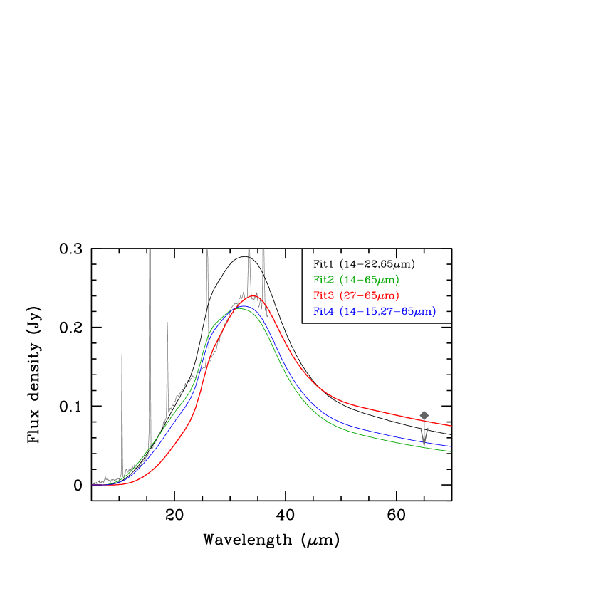
Figure 12: Reproduced SEDs by the Equation (7) (black, green, red, and blue lines) overlaid on the Spitzer/IRS spectrum of Wray16-423 (grey line). The point indicated by the diamond shows the upper-limit flux density at AKARI/FIS 65 $\mu$m. Fits 1-4 are different in terms of the fitting wavelength range. The fitting results are summarised in Table 5.

Table 5: Fitting results for the broad 30 $\mu$m feature. The uncertainty of $T_{d}$(max) is within 0.6 K.

Fitting	Fitting wavelength	$T_{d}$(max)
	($\mu$m)	(K)
Fit1	14-22,65	145.5
Fit2	14-65	131.3
Fit3	27-65	108.1
Fit4	14-15, 27-65	133.0

Our PNe display a broad 30 $\mu$m feature, which has been seen in many C-rich objects. Hony et al. (2002a) performed a comprehensive analysis of the 30 $\mu$m feature showing objects with ISO/SWS spectra. Due to the wavelength coverage, our measured FWHMs were narrower than the measurements of Hony et al. (2002a, $\sim$10 $\mu$m). Hony et al. (2002a) argued that the feature originated from a CDE MgS. The CDE MgS has been the major candidate for the 30 $\mu$m feature. However, as we introduced earlier, the origin of this feature is unclear.

Messenger et al. (2013) performed a detailed analysis on the 30 $\mu$m and the 11 $\mu$m SiC features; the authors concluded that the 30 $\mu$m feature is likely due to a carbide or sulfide component, and that the abundance of the carrier of the 30 $\mu$m feature is linked to SiC abundance. This conclusion seems to agree with Sloan et al. (2014), who argued that the MgS feature strength climbs just as the SiC strength drops, as the dust shells around the stars become red, based on the assumption that the SiC/amorphous carbon is coated by MgS as the dust grains move away from the central star. Laboratory experiments by Lodders & Fegley (1995) revealed the condensation temperatures of different C/O ratios and pressures; for the case of C/O = 2.0 and a total pressure of 10^-3 bar, the condensation temperatures of graphite, SiC, and MgS grains are 1978 K, 1736 K, and 1152 K, respectively.

We measured the $F$(11 $\mu$m SiC)/$F$(IR) for LMC PNe LMC8, 25, 48, and 85 (Table 16) showing SiC. Among these PNe, an anti-correlation relationship exists between the SiC and 30 $\mu$m intensities (correlation factor=–0.88), supporting the idea of Sloan et al. (2014). We investigated the effective temperatures of 14 LMC PNe using Cloudy. The average effective temperature of the four SiC-containing PNe (LMC8, 25, 48, and 85) is 50 750 K, while a value of 123 000 K is determined among the non-SiC containing PNe (LMC19, 78, and 99, and Wray16-423). The CSPNe of SiC-containing PNe seem to be cooler and younger than those of the non-SiC-containing PNe. Thus, the MgS grains in non-SiC-containing PNe may be far from the central stars. In comparison, the average $\lambda_{c}$s of the 30 $\mu$m feature in SiC-containing four PNe is 30.50 $\mu$m and that in the remaining non-SiC-containing four PNe is 31.73 $\mu$m.

However, Zhang et al. (2009) cast doubt on this identification for the 30 $\mu$m feature. They demonstrated that the MgS mass of (0.96-7.16)$\times$10^-5 M_⊙, formed from the available S atoms, could not account for the observed strength of the 30 $\mu$m feature in the proto-PN HD56126, even if all the dust grains existed as MgS (the required MgS mass is $>$3.5$\times$10^-4 M_⊙).

CDE iron-rich sulphide, such as Mg_0.5Fe_0.5S (Fe50S), also show a broad feature around 30 $\mu$m, similar to the CDE MgS feature (Messenger et al., 2013). In PNe, Henry et al. (2012) reported no correlation between the S abundance deficiency and the occurrence of the broad 30 $\mu$m feature, implying that iron-rich sulfide rather than MgS may be favored as a carrier of the 30 $\mu$m feature. The type of Mg-Fe-S grains that form depends on the amount of Mg, Fe, and S atoms in the solid phase.

Another possible candidate for the 30 $\mu$m feature is graphite, as proposed by Jiang et al. (2014). The opacity of graphite by Draine & Lee (1984) exhibits broad emission (FWHM$>$60 $\mu$m) peaked at $\sim$30-40 $\mu$m. The theoretical opacity of graphite with a d.c. conductivity of 100 $\Omega$^-1 cm^-1 by Jiang et al. (2014) shows a well-consistent FWHM of $\sim$10 $\mu$m to the observed FWHMs reported by Hony et al. (2002a). Otsuka et al. (2014) found that the relative strength of the 30 $\mu$m feature to the underlying continuum in fullerene C₆₀-containing PNe is constant; they also succeeded in fitting both the 30 $\mu$m feature and the 13-160 $\mu$m continuum using the synthesised absorption efficiency $Q_{\mathrm{abs}}(\lambda)$, derived from the combined data of ISO/SWS/LWS and Spitzer/IRS spectra of C₆₀-containing PN IC418. Their derived opacity curve is similar to that of graphite by Draine & Lee (1984), with the exception of the feature strength and FWHM. Otsuka et al. (2014) concluded that the 30 $\mu$m feature and featureless continuum may be related to hydrogenated amorphous carbon (HAC) or graphite. HAC has two resonances centered at $\sim$20 $\mu$m and $\sim$30 $\mu$m as demonstrated in Fig. 9 of Otsuka et al. (2013). However, since its optical constant is strongly variable for different chemical and physical conditions such as hydrogen-content and grain size, one might be able to reproduce the strong 30 $\mu$m feature plus the weaker sub structures.

We utilised the method of Otsuka et al. (2014) to verify our ability to fit the $\geq$14 $\mu$m SED of Wray16-423 with their $Q_{\mathrm{abs}}(\lambda)$ even if it will not be possible to fit the broad 16-24 $\mu$m feature in this way. The model of Otsuka et al. (2014) assumes that the dust density, as a function of the distance from the CSPN $r$, is distributed around the CSPN with a power-law ($\propto r^{-p}$) and that the dust temperature distribution $T_{d}$($r$) also follows a power-law ($\propto r^{-q}$). The thermal radiation from spherical grains can be estimated by the following:

$$F_{\lambda}=C\cdot Q_{\mathrm{abs}}(\lambda)\int^{T_{d}(\mathrm{max})}_{T_{d}(\mathrm{min})}T_{d}^{-\alpha}B_{\lambda}(T_{d})~{}dT_{d},$$ (7)

where $C$ is a constant value, $T_{d}({\mathrm{max}})$ and $T_{d}({\mathrm{min}})$ are the maximum and minimum temperatures of the 30 $\mu$m feature, respectively, $\alpha$=$(3-p)/q>0$, and $B_{\lambda}(T_{d})$ is the Plank function. We chose both $p$ and $q$ to be 2. The fit is not sensitive to $T_{d}({\mathrm{min}})$; thus, we let $T_{d}({\mathrm{min}})$=20 K, a temperature more or less characteristic of dust in the ISM.

We fit the Spitzer/IRS spectrum for wavelengths longer than 14 $\mu$m by the Equation (7). As a constraint to set the upper limit flux density over 36.5 $\mu$m by the model fit, we used an upper limit flux density $I_{\nu}$(65 $\mu$m)=88.3 mJy measured from the AKARI/FIS Far-infrared All-Sky Survey Maps. We performed four fits, as summarised in Table 5. The fitting regions of each differed. The resultant SEDs are plotted on the Spitzer/IRS spectrum in Figure 12. Fit1 - a test whether the 14-22 $\mu$m dust continuum is linked with the 30 $\mu$m feature - predicts $\sim$1.2 times larger flux density at the peak of the 30 $\mu$m feature. Fit2 converging at 14-65 $\mu$m gives a better result; however, it cannot explain $\sim$20-24 $\mu$m of the broad 16-24 $\mu$m feature or the 30 $\mu$m. Fit3, focusing only the 30 $\mu$m feature, provides a good fitting for the 30 $\mu$m feature, although it under-predicts the flux density below 27 $\mu$m. Fit4 skips the broad 16-24 $\mu$m feature and gives results similar to those obtained in Fit2.

Our simple analysis demonstrates that the broad 16-24 $\mu$m in Wray16-423 is unrelated to the 30 $\mu$m feature. If we focus on the 27 $\mu$m or longer wavelength data, we can reproduce part of the observed 30 $\mu$m feature with the synthesised $Q_{\mathrm{abs}}(\lambda)$ of Otsuka et al. (2014). More fits to the 30 $\mu$m feature showing PNe (but without broad 16-24 $\mu$m feature) are necessary to synthesize the absorption efficiency of the 30 $\mu$m feature for astronomical objects and to separate the 16-24 $\mu$m feature from the complex of 16-24 $\mu$m and 30 $\mu$m features.

3.7 SED modeling

Figure 13: Radial profile of the hydrogen density adopted in SED modeling.

Table 6: Best fitting parameters and the derived properties by the Cloudy model.

Parameters of the CSPN	Values
$L_{\ast}$	4753 L⊙
$T_{\rm eff}$	110 110 K
$M_{V}$	2.691
$\log\,g$	6.0 cm s-2
Distance	24.8 kpc
Parameters of the Nebula	Values
Abundances	He:11.02, C:8.86, N:7.69, O:8.22, Ne:7.50,
($\log_{10}$(X/H)+12)	S:6.40, Cl:4.71, Ar:5.92, K:4.31, Fe:5.57
	[Si,Mg/H]=–2.00, Others:[X/H]=–0.65
Geometry	Spherical
Shell size	$R_{\rm in}$=0.20″ (0.02 pc), $R_{\rm out}$=1.3″ (0.16 pc)
$n_{\rm H}$	See Fig.13
filling factor	0.85
$\log I$(H$\beta$)	–11.705 erg s-1 cm-2 (de-reddened)
$m_{\rm g}$	0.59 M⊙
Parameters of the Dust	Values
Composition	3.1 $\%$ PAHs and 96.9 $\%$ graphite (mass frac.)
Grain size	0.0004-0.011 $\mu$m for PAH
	0.005-0.25 $\mu$m for graphite
$T_{d}$	113-305 K (PAHs), 43-194 K (graphite)
$m_{d}$	1.32(–4) M⊙ in total
$m_{d}$/$m_{\rm g}$	2.26(–4)

We constructed an SED model to investigate the physical conditions of the gas and dust grains, in order to derive their masses using Cloudy c10.00.

3.7.1 Model approach

We set the distance to Wray16-423 to 24.8 kpc for comparison with the observed fluxes and flux densities. For the incident SED from the CSPN, we adopted the model grids of non-LTE line-blanketed, plane-parallel, hydrostatic model atmospheres of halo stars ([Z/H]=–1) by Rauch (2003). Because the He ii line-fluxes are sensitive to the surface gravity $\log$ $g$, we tested small gas-only model grids with varying $\log$ $g$ that matched the flux of the He ii $\lambda$ 4686 Å. In the small grids, we set the CSPN’s effective temperature to $T_{\rm eff}$=110 660 K and luminosity $L_{\ast}$ to 4683 L_⊙ using Equations (3.1) and (3.2) of Dopita & Meatheringham (1991), which are established amongst Magellanic Cloud PNe, assuming optically thick nebula. Accordingly, we set $\log$ $g$ to 6.0 cm s^-2. We kept this surface gravity in the gas+dust full SED model, and adopted the above $T_{\rm eff}$ and $L_{\ast}$ as a first guess.

For gas-phase elemental abundances, we adopted the observed values listed in Table 4 as the first guess, and refined these to match the observed line intensities of each element. We considered the CEL O line fluxes to set the O abundance. We adopted the same transition probabilities and effective collision strengths of CELs used in our plasma diagnostics and abundance determinations. Because Cloudy does not include any Kr lines, we did not consider this element. The abundances for non-calculated elements, except for Mg and Si, were held constant at [X/H]=–0.65, which is the average between the observed [Cl/H] and [Ar/H]. Because the deficiency of refractory elements Mg and Si is unknown, we adopted [Mg,Si/H]=–2.

We determined the radial H-density profile of the nebula, based on the radial intensity profile of the HST/WFPC2 F656N image using an Abel transformation under the assumption of spherical symmetry. The ionization-bound models over-predicted the [N ii] and [O ii] lines and under-predicted the [O iii] lines, whereas the matter-bound models gave better fit to the observed fluxes of these emission lines. Therefore, we assumed the matter-bound condition. The outer radius $R_{\rm out}$ was set to 1.3^′′ (0.16 pc) and the inner radius $R_{\rm in}$ was 0.2^′′ (0.023 pc), from the HST image. We adopted a constant filling factor of 0.85. The adopted radial profile of the hydrogen density is presented in Figure 13. Our set hydrogen density profile appeared to be similar to the photoionisation models without dust grains by Dudziak et al. (2000), who adopted the constant hydrogen densities of 9500 cm^-3 for 0.023-0.051 pc (covering factor =0.17) and 3600 cm^-3 for 0.023-0.08 pc (0.83).

We attempted to fit the observed SED in the range from 0.1516 $\mu$m (GALEX-Fuv) to 65 $\mu$m (AKARI/FIS), assuming that the infrared excess around 5-40 $\mu$m was due to the emission from PAH molecules and carbon-based grains. There are no suitable optical constants for the broad 16-24 $\mu$m and 30-$\mu$m features; thus, we skipped these bands. The 16-24 $\mu$m and 27.4-36.5 $\mu$m SEDs were out of the fitting range in the model. Here, we adopted graphite and PAH. We assumed a spherical shape for both the graphite and PAH. In graphite, the spheres were assumed to be randomly oriented, and the ”1/3-2/3” approximation was utilised (for validity of this approximation see, Draine & Malhotra, 1993). The optical constants were taken from Draine & Li (2007) (PAH-Carbonaceous grains) for PAH and Draine & Lee (1984) for graphite. For PAH, we adopted the radius $a$ in the range from 0.0004 (30 C-atoms) to 0.0011 $\mu$m (500 C-atoms) with the standard interstellar dust-grain size distribution by Mathis et al. (1977) (i.e., $a^{-3.5}$). For the graphite, we adopted the same size distribution with $a$=0.005-0.25 $\mu$m.

To verify the model fitting accuracy, we evaluated the chi-square value (${\chi}^{2}$) from the 44 gas emission fluxes, 9 gas-phase abundances, 7 broad band fluxes, and the 9 de-reddened flux densities $I_{\nu}$ from GALEX, HST/WFPC2, 2MASS, and WISE bands. We used the AKARI/FIS $I_{\nu}$(65 $\mu$m) to set the dust continuum above 36.5 $\mu$m.

3.7.2 Comments on SED model results

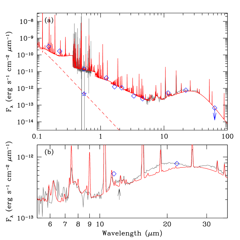
Figure 14: (upper panel) Predicted SED of the PN Wray16-423 by Cloudy modeling (the red solid line and the dashed line). The red solid line is the emergent model spectrum of the CSPN plus the nebula, and the dashed line is the spectrum of the CSPN. The grey lines are the observed spectra taken by the Subaru/HDS and the Spitzer/IRS. The blue diamonds are the photometry data of the CSPN plus the nebula from the GALEX (Fuv and Nuv bands), HST (F547M), 2MASS (near-IR $JHKs$), WISE (11.6 and 22.1 $\mu$m), and AKARI/FIS 65 $\mu$m. The green star is the photometry of the CSPN measured by the HST/(F547M) image. (lower panel) Closed-up plot for mid-IR wavelengths. The spectral resolving power ($R$) of the Cloudy model spectrum was constant (100) to match that of the Spitzer/IRS. The lack of emission, indicated by the arrow, could be filled by adding amorphous carbon grains in the model. See the text for details.

Table 7: Comparison between SED modeling and observations.

Ion	$\lambda_{\rm lab}$	$I$(CLOUDY)	$I$(Obs)	Ion	$\lambda_{\rm lab}$	$I$(CLOUDY)	$I$(Obs)
		($I$(H$\beta$)=100)	($I$(H$\beta$)=100.0)			($I$(H$\beta$)=100.0)	($I$(H$\beta$)=100.0)
[O ii]	3726 Å	19.79	19.52	He i	5876 Å	16.22	15.20
[O ii]	3729 Å	14.17	10.72	[S iii]	6312 Å	1.19	1.42
[Ne iii]	3869 Å	87.36	85.71	[N ii]	6548 Å	5.45	5.50
[Ne iii]	3968 Å	26.33	26.15	H$\alpha$	6563 Å	284.8	285.0
[S ii]	4069 Å	0.63	1.11	[N ii]	6584 Å	16.08	16.20
C iii	4187 Å	0.17	0.15	He i	6678 Å	4.19	3.98
C ii	4267 Å	0.45	0.47	[S ii]	6716 Å	1.82	1.58
H$\delta$	4341 Å	46.69	46.90	[S ii]	6731 Å	2.26	2.64
[O iii]	4363 Å	14.59	13.39	[Ar iii]	7135 Å	7.77	10.83
He i	4388 Å	0.63	0.57	He i	7281 Å	1.06	1.01
He i	4471 Å	5.20	5.10	[O ii]	7323 Å	1.56	2.79
[Fe iii]	4701 Å	0.013	0.022	[O ii]	7332 Å	1.24	2.15
[Ar iv]	4711 Å	2.81	1.86	[Ar iii]	7751 Å	1.88	2.71
[Ar iv]	4740 Å	3.72	2.71	[Cl iv]	8047 Å	0.34	0.56
C iii	4649 Å	0.48	0.40	[S iii]	9069 Å	4.65	7.99
C iv	4659 Å	0.045	0.103	[S iv]	10.51 $\mu$m	55.07	27.80
He ii	4686 Å	10.02	11.14	[Ne ii]	12.80 $\mu$m	0.21	1.07
H$\beta$	4863 Å	100.0	100.0	[Ne iii]	15.55 $\mu$m	49.05	59.76
[Fe iii]	4881 Å	0.032	0.032	[S iii]	18.67 $\mu$m	7.65	9.92
He i	4922 Å	1.37	1.27	[O iv]	25.88 $\mu$m	16.00	11.92
[O iii]	4931 Å	0.14	0.14	[S iii]	33.47 $\mu$m	3.99	4.31
[O iii]	4959 Å	336.3	362.4	[Ne iii]	36.01 $\mu$m	4.03	3.87
[O iii]	5007 Å	1012.1	1062.1	IRS-1	6.20 $\mu$m	12.36	13.466
[Ar iii]	5192 Å	0.12	0.13	IRS-2	6.90 $\mu$m	11.29	13.96
[Fe iii]	5271 Å	0.064	0.040	IRS-3	7.90 $\mu$m	18.95	18.22
[Cl iv]	5324 Å	0.012	0.021	IRS-4	11.30 $\mu$m	19.45	19.28
[Cl iii]	5518 Å	0.28	0.25	IRS-5	12.30 $\mu$m	19.47	21.30
[Cl iii]	5538 Å	0.31	0.37	IRS-6	13.50 $\mu$m	40.31	40.70
[N ii]	5755 Å	0.45	0.40	IRS-7	14.50 $\mu$m	21.20	20.52
Band	$\lambda_{\rm c}$	$I_{\nu}$(CLOUDY)	$I_{\nu}$(Obs)	X		$\log_{10}$(X/H)CLOUDY	$\log_{10}$(X/H)Obs
		(mJy)	(mJy)			+12	+12
GALEX-Fuv	1516 Å	5.61	2.58	He		11.02	11.02
GALEX-Nuv	2267 Å	3.96	3.07	C		8.86	8.92
WFPC2/F547M	5484 Å	1.35	1.44	N		7.69	7.69
2MASS-$J$	1.235 $\mu$m	2.49	2.13	O		8.22	8.31
2MASS-$H$	1.662 $\mu$m	1.60	1.15	Ne		7.50	7.61
2MASS-$Ks$	2.159 $\mu$m	2.47	1.68	S		6.40	6.40
WISE-B1	3.353 $\mu$m	1.90	1.32	Cl		4.71	4.74
WISE-B2	4.603 $\mu$m	2.87	1.69	Ar		5.92	6.00
WISE-B3	11.56 $\mu$m	23.79	23.68	Fe		5.57	5.56
AKARI/FIS	65 $\mu$m	88.30	$<$88.33	${\chi}^{2}$(reduced ${\chi}^{2}$)			48.14(0.63)

Note – The values for the IRS-1, 2, 3, 4, 5, 6, and 7 bands correspond to integrated fluxes between the following wavelength ranges, 5.9-6.9 $\mu$m, 6.4-7.4 $\mu$m, 7.4-8.4 $\mu$m, 10.8-11.8 $\mu$m, 11.8-12.8 $\mu$m, 12.5-14.5 $\mu$m, and 14-15 $\mu$m, respectively.

The properties of the CSPN, nebula, and dust/molecules matching the observed quantities are listed in Table 6. The predicted fluxes relative to the H$\beta$, the flux densities at the interest bands, and elemental abundances compared with observations are listed in Table 7. The reduced chi-square value indicates that our SED model can reproduce the observed quantities.

We may have overestimated the [Ne ii] $\lambda$ 12.80 $\mu$m in the low-dispersion Spitzer/IRS spectrum, because this line would be contaminated by the 12.7 $\mu$m PAH (see Fig. 9). Although we could not reproduce these line fluxes within estimated errors, our model is globally successful in explaining the observations. Although without the UV spectra we cannot say for certain, the large difference in GALEX-Fuv and Nuv might be due to the adopted extinction value and reddening correction function for GALEX wavelength.

The model predicted $M_{V}$ of the CSPN (2.685) is consistent with the observed absolute magnitude of 2.770$\pm$0.2 in the case of 24.8 kpc within error. The uncertainty of $T_{\rm eff}$ is 2 000 K. Taking into account the distance uncertainty of 0.8 kpc (Kunder & Chaboyer, 2009), our derived $L_{\ast}$ of 4753$\pm$1230 L_⊙ is fairly consistent with Dudziak et al. (2000), who reported 4350$\pm$150 L_⊙ and $T_{\rm eff}$=107 000$\pm$10 000 K. The uncertainties of the predicted elemental abundances are within 0.1 dex.

Taking the absolute Spitzer/IRS flux calibration uncertainty $\sim$17 $\%$ (Decin et al., 2004), the dust mass $m_{d}$ would be (1.32$\pm$0.23)$\times$10^-4 M_⊙. The uncertainty of the dust mass fraction would be within $\pm$1,$\%$. The estimated dust mass here would be the lower limit value, because we skipped the broad 16-24 $\mu$m and 30 $\mu$m bands. If one of the carriers for the 30 $\mu$m broad band is the Fe-rich sulfide, then the dust mass and the dust-to-gas mass ratio could increase. Indeed, the large Fe depletion with respect to Ar is confirmed; thus, the missing Fe atoms would exist as Fe dust grains. In the next section, we discuss how much dust mass can be added if the broad 30 $\mu$m feature is from Fe-rich sulfide or MgS. The gas mass $m_{g}$ (the sum of the ionised and atomic gas mass within the volume occupied within $R_{\rm out}$) is 0.59$\pm$0.10 M_⊙. We also ran the model for the case of $R_{\rm out}$=1.0″ (0.12 pc), and we obtained the $m_{d}$=(1.05$\pm$0.18)$\times$10^-4 M_⊙ and $m_{g}$=0.45$\pm$0.08 M_⊙. The estimated $m_{g}$ for our $R_{\rm out}$=1.0″ and 1.5″ models is consistent with the result of 0.4 M_⊙ by Zijlstra et al. (2006a). The ionised gas mass exceeds the prior estimate of 0.248 M_⊙ by Dudziak et al. (2000), which we attribute to the difference in H$\beta$ flux and outer radius ($\log$ $I$(H$\beta$)=–11.89 erg s^-1 cm^-2 and $R_{\rm out}$=0.08 pc at 25 kpc). If we adopted their $I$(H$\beta$), then $m_{g}$ is $\sim$0.29 M_⊙ in the case of $R_{\rm out}$=0.12 pc.

The dust mass in Wray16-423 is similar to that in Hen2-436 ((2.9-4.0)$\times$10^-4 M_⊙, Otsuka et al., 2011), whereas the gas mass is 8-12 times larger. Otsuka et al. (2011) and Dudziak et al. (2000) estimated 0.05-0.07 M_⊙ (ionised + neutral gas) and 0.04 M_⊙ (ionised gas) for Hen2-436, respectively. Dudziak et al. (2000) argued that the outer boundary in Hen2-436 is determined by radiation (ionisation bound). Indeed, Hen2-436 is very compact; its outer radius is $\sim$0.03 pc. The small O²⁺/(O⁺+O²⁺) ratio in Hen2-436 (0.85, Otsuka et al., 2011) seems to support this (c.f., 0.96 in Wray16-423).

In Figure 14a, we present the observed SED plots (blue diamonds and grey lines) and the modelled SED (red line). The dashed line is the modelled incident SED of the CSPN, where the flux density in the F574M band is consistent with the observed value. In Figure 14b, we display a close-up of the SED in the wavelength range covered by the Spitzer/IRS spectrum. The large mass fraction of the graphite grains is due to the rising mid-IR flux density toward $\sim$25 $\mu$m. Because we did not consider the possibility of very large PAH molecules discussed in Section 3.6.3, the 15-20 $\mu$m PAH plateau is not reproduced by the model. The complex of the 10-14 $\mu$m PAHs and broad 11 $\mu$m feature in Wray16-423 could be reproduced with PAHs although the fitting is not perfect. The observed band profile of the 10-14 $\mu$m PAHs and broad 11 $\mu$m feature is nearly flat top around 12 $\mu$m whereas the predicted band profile is very similar to the observed one except for the small lack of emission indicated by the arrow. The lack of emission could be filled if we add amorphous carbon grains in the model, because the $Q_{abs}$($\lambda$) of amorphous carbon calculated from the optical data of Rouleau & Martin (1991) appears in a small bump around 12 $\mu$m.

4 Discussion

4.1 Progenitor mass estimate by comparison to AGB nucleosynthesis models

Table 8: Comparison to AGB nucleosynthesis models of Karakas (2010). The C abundance in Wray16-423 is the RL C value. See text regarding the estimate of the Mg abundance in Section 4.2. The core-mass of Wray16-423 was estimated from Vassiliadis & Wood (1994).

	AGB models
	1.5 M⊙	1.75 M⊙	1.90 M⊙	Present
	$Z$=0.004	$Z$=0.004	$Z$=0.004	work
He	10.97	10.98	10.99	11.02$\pm$0.04
C	8.46	8.80	8.94	8.92$\pm$0.08
N	7.65	7.69	7.71	7.69$\pm$0.04
O	8.23	8.25	8.25	8.31$\pm$0.01
Ne	7.42	7.51	7.61	7.61$\pm$0.03
Mg	6.88	6.88	6.89	6.19$\pm$0.30
S	6.69	6.70	6.70	6.40$\pm$0.03
Fe	6.78	6.78	6.78	5.56$\pm$0.07
Ejected mass	0.04 M⊙	0.15 M⊙	0.44 M⊙	0.59$\pm$0.10 M⊙
Core-mass	0.62 M⊙	0.63 M⊙	0.64 M⊙	0.62-0.67 M⊙

Because the HDS spectrum shows a signature of [WC] CSPN in the C iv $\lambda\lambda$ 5801/12 Å band, the CSPN could be He-rich. Assuming that the CSPN is in the midst of He-burning, comparing the estimated $L_{\ast}$ and $T_{\rm eff}$ on He-burning post-AGB evolution tracks with the initial $Z$=0.008 of Vassiliadis & Wood (1994) indicates a progenitor mass of 1.5-2.0 M_⊙.

The presence of the C iv $\lambda\lambda$ 5801/12 Å band could be evidence that Wray16-423 experienced a very late thermal pulse (VLTP). Vassiliadis & Wood (1994) demonstrated the He-burning post-AGB track for initially 1.5 M_⊙ stars, with $Z$=0.008; these stars experienced a VLTP at $\log_{10}$$T_{\rm eff}$$\sim$4.9 ($\sim$79 430 K). The subsequent evolution was dominated by He-shell burning. The difference from normal He-burning evolution tracks is that there is no upturn luminosity, and the evolution after VLTP is very similar to the H-burning tracks. If Wray16-423 experienced a VLTP, then the progenitor mass is estimated to be $>$1.5 M_⊙.

Next, we verify whether AGB nucleosynthesis models can explain observed elemental abundances in an initial $\sim$1.5-2.0 M_⊙ star. In Table 8, we compare the AGB model results of Karakas (2010) with our observation results. The ¹³C pocket mass is not included. Besides He/C/N/O/Ne/S/Fe abundances, we list the ejected mass at the last thermal pulse and the core-mass of the CSPN in the last two lines of Table 8. Here, we assume that the estimated gas mass through our SED model is nearly equal to the ejected mass at the last thermal pulse. The gas mass estimated in our SED models depends on the outer nebula radius and the de-reddened H$\beta$ flux. So far, the gas mass estimates in Wray16-423 range from 0.248 M_⊙ (Dudziak et al., 2000) to 0.49$\pm$0.10 M_⊙ (see section 3.7.2). Among these model predictions, the 1.9 M_⊙ model provides an excellent fit to the observed elemental abundances and the ejected mass. The consistency between the observed and the predicted Ne abundances indicates that the ¹³C pocket may not form in Wray16-423. Even if we adopt the expected CEL C abundance of 8.70$\pm$0.14, as described in section 3.4, our conclusion does not change considerably.

4.2 Expected solid-phase Mg, S, and Fe

The difference between the observed S and Fe abundances and the AGB model predicted abundances could constrain how much mass of each element could be locked by the dust grains, based on the assumption that elemental abundances in the nebula are consistent with the predicted values in the case of the 1.9 M_⊙/$Z$=0.004 AGB model. The density fraction of an element X in the solid phase, $n_{\rm solid}$(X)/$n$(X), can be roughly estimated using the following:

$$\frac{n_{\rm solid}({\rm X})}{n({\rm X})}=1-10^{\log_{10}\left(\frac{n({\rm X})}{n({\rm H})}\right)_{\rm obs}-\log_{10}\left(\frac{n({\rm X})}{n({\rm H})}\right)_{\rm model}},$$ (8)

where $\log_{10}$($n(X)$/$n$(H))_obs and $\log_{10}$($n$(X)/$n$(H))_model are the observed and the AGB star model predicted elemental abundances of the element X. Using the Equation (8), $\sim$92-95 $\%$ of the Fe atoms and $\sim$46-53 $\%$ of the S atoms in the nebula could be in the solid phase.

The ionised Mg abundances in PNe have been calculated using the forbidden lines at UV wavelengths and recombination Mg ii $\lambda$ 4481 Å. We were unable to detect optical Mg ii lines. Instead, we attempt to estimate the gas-phase Mg abundance using Mg⁰ and N⁰ abundances based on the assumption that all N atoms exist as a gas. This assumption is possible, because the observed N abundance (7.69$\pm$0.04) is consistent with AGB model predictions (7.71). Under the assumption that Mg-containing grains did not form, the Mg/N ratio would be 0.151 from the 1.9 M_⊙ AGB model; thus, nearly identical to Mg⁰/N⁰. In this case (i.e., Mg-atoms are not depleted by dust grains), the Mg⁰/H⁺ should be 0.151$\times$N⁰/H⁺ = 8.98(–8)$\pm$4.92(–9). Because the actual Mg⁰/H⁺ is 1.81(–8)$\pm$5.27(–9), about 14-26 $\%$ of the Mg-atoms likely exist as a gas and the remaining 74-86 $\%$ are in the solid phase. Using the modeled Mg/H of 6.89 dex (7.76(–6) in linear scale), the gas-phase Mg/H would be 6.19$\pm$0.30 dex (1.53(–6)$\pm$4.63(–7) in linear scale). Both the gas and solid phase Mg estimates are optimistic and depend on the AGB model prediction. UV Mg forbidden lines in HST/STIS spectra would provide a more exact value.

Using the estimated fractions of the solid phase Mg, S, and Fe atoms, we estimate the solid-phase masses $m_{\rm solid}$(X) using the following equation:

$$m_{\rm solid}({\rm X})=\mu({\rm X})\cdot\frac{m_{g}}{1+4~{}n({\rm He})/n({\rm H})_{\rm obs}}\cdot\frac{n({\rm X})}{n({\rm H})}_{\rm model}\cdot\frac{n_{\rm solid}({\rm X})}{n({\rm X})},$$ (9)

where $\mu$(X) is the atomic mass, and $n$(He)/$n$(H)_obs is the He number density (1.06(–1), See Table 4).

In summary, $\sim$92–95% of the Fe atoms, $\sim$74–86% of the Mg and $\sim$46–53% of the S atoms in the nebula could be in the solid phase, corresponding to masses of respectively 1.3$\pm$0.2, 0.7$\pm$0.2 and 0.33$\pm$0.01 $\times 10^{-4}$ M_⊙.

4.3 Can MgS or Fe50S grains explain the 30 $\mu$m feature?

Table 9: Required MgS and Fe50 grain masses for the 30 $\mu$m feature. The maximum Fe50S (Mg_0.5Fe_0.5S) and MgS mass could form 7.65(–5) M_⊙ and 5.95(–5) M_⊙, respectively.

Models	$T_{d}$(MgS)	$T_{d}$(Fe50S)	$m_{d}$(MgS)	$m_{d}$(Fe50S)
	(K)	(K)	(M⊙)	(M⊙)
Case 1	133.8$\pm$0.9	117.9$\pm$1.2	5.5(–7)$\pm$1.0(–7)	1.8(–6)$\pm$3.2(–7)
Case 2	′′	′′	6.0(–6)$\pm$1.1(–6)	1.9(–5)$\pm$3.6(–6)

In largely Fe-depleted C-rich PNe, such as Wray16-423, estimated carbon dust masses may make up a portion of the dust grains in the nebula, not including the broad 16-24 $\mu$m and 30 $\mu$m features. As discussed in Section 3.6.4, Mg-Fe-S grains may form in the dusty nebula of Wray16-423, and could be a carrier for the broad 30 $\mu$m feature. Mg-Fe-S grain masses are controlled by the solid-phase S-atom mass. Adopting the solid-phase Mg, S, and Fe masses as we estimated above, the possible maximum Fe50S (Mg_0.5Fe_0.5S) and MgS masses could form 7.65(–5) M_⊙ and 5.95(–5) M_⊙, respectively.

As such, can MgS or Fe50S grains explain the 30 $\mu$m feature? To answer this question, we estimate their masses using the Plank function with a single dust temperature method described in Hony et al. (2003), who explained that the dust mass $m_{d}$ in the optically thin nebula can be estimated using the following equation:

$$m_{d}=\frac{4}{3}\,F_{\lambda_{0},\lambda_{1}}\,D^{2}\,\rho\,\left(\int_{\lambda_{0}}^{\lambda_{1}}\frac{Q_{abs}(\lambda,a)}{a}\,B_{\lambda}(T_{d})\,d\lambda\right)^{-1},$$ (10)

where $F_{\lambda_{0},\lambda_{1}}$ is the integrated flux in the wavelength range from $\lambda_{0}$ to $\lambda_{1}$. Here, we adopt the central wavelength and FWHM listed in Table 15 of Appendix C. $\lambda_{0}$ and $\lambda_{1}$ are 28 $\mu$m and 36 $\mu$m, respectively, $D$ is the distance (24.8 kpc), and $\rho$ is the grain density, 3 g cm^-3 for MgS and 5 g cm^-3 for Fe50S. When the grain radius is small in comparison with the wavelength $\lambda$, the absorption profile becomes independent of $a$ (Pegourie, 1988). We calculated the $Q_{abs}$($\lambda$)/$a$ values of the CDE MgS and Fe50S by following Equation (4) of Fabian et al. (2001). The optical data of MgS (Mg_0.9Fe_0.1S, actually) and Fe50S (Mg_0.5Fe_0.5S) were taken from Begemann et al. (1994).

In the models, we use an average dust temperature for both MgS and Fe50S derived by Plank function fitting with a single temperature. For $F_{\lambda_{0},\lambda_{1}}$, we consider two cases: (Case 1) the underlying continuum of the 30 $\mu$m feature is largely from graphite, as demonstrated in the Cloudy model, and (Case 2) instead of graphite, the contribution comes from amorphous carbon, whose absorption efficiency drops sharply for longer wavelengths, compared with graphite; thus, MgS or Fe50S may be the main contributors to this band radiation. For Case 1, we calculated $F_{\lambda_{0},\lambda_{1}}$ of 4.88(–13) erg s^-1 cm^-2 using the residual spectrum generated by subtracting the Cloudy synthesised spectrum from the observed Spitzer/IRS spectrum. For Case 2, we calculated $F_{\lambda_{0},\lambda_{1}}$ of 5.33(–12) erg s^-1 cm^-2 from the observed Spitzer/IRS spectrum (the Cloudy spectrum was not subtracted).

The required masses to produce the band flux of the 30 $\mu$m feature are listed in the last column of Table 9. If the graphite grains exist in the nebula (Case 1), then the required MgS or Fe50S mass is less than the possible maximum MgS and Fe50S masses. Even if not graphite but amorphous carbon are the main dust grains in the nebula, MgS and Fe50S grains can reproduce the intensity peak of the observed broad 30 $\mu$m feature (Case 2).

At present, we hold onto the possibility that MgS and Fe50S are carriers of the 30 $\mu$m feature in the case of Wray16-423. By adding the 1.8(–6)$\pm$3.2(–7) M_⊙ of Fe50S, we could estimate the maximum dust mass to be 1.6(–2) M_⊙. However, we understand that these estimates are optimistic, given that we did not consider S-atom-based molecules, such as CS. If any sulfide molecules form in the nebula, then it would be more difficult to explain the 30 $\mu$m feature with Fe50S and MgS. If it is possible to estimate the mass of the S-atom existing as the molecule with sub-mm spectra and the optical characteristics data of MgS, Fe50S and the new graphite data by Jiang et al. (2014) are available over a wider wavelength range, then it may be possible to resolve which grains carry the 30 $\mu$m feature.

5 Summary

We performed a detailed chemical abundance and dust analysis of Sgr dSph PN Wray16-423. Numerous gas emission lines were detected, from which the abundances of 11 elements were calculated. The [Kr/H] and [Fe/H] abundances were comparable to Sgr dSph PN Hen2-436, which has a similar metallicity. The [Kr/O] abundance was consistent with the value expected by the [Kr/O]-C/O relation found amongst Galactic PNe. The extremely small [Fe/H] does not reflect the metallicity, but it implies that most of the Fe atoms would be in the solid phase, given the [Ar/H] abundance. The Spitzer/IRS spectrum displays broad 16-24 $\mu$m and 30 $\mu$m features, as well as PAH bands at 6-9 $\mu$m (Class $\mathcal{B}$) and 10-14 $\mu$m (Class $\alpha$). An unidentified broad feature in $\sim$16-24 $\mu$m is probably unrelated to FeS, amorphous silicate, and PAH. The progenitor was estimated to be a $\sim$1.5-2.0 M_⊙ star. The observed elemental abundances and the derived gas mass were in good agreement with the AGB nucleosynthesis model for an initial mass of 1.90 M_⊙ and a $Z$=0.004 star. We found that about 80 $\%$, 50 $\%$, and 90 $\%$ of the Mg, S, and Fe atoms were likely in the solid phase, respectively. Using the derived solid-phase Mg, S, and Fe masses, we estimated the possible maximum MgS and Fe50S grain masses. We tested whether MgS and Fe50S grains can produce the intensity peak of the observed broad 30 $\mu$m band with these masses. Depending on the total sulfide molecule masses, at present, MgS and Fe50S could be carriers of the 30 $\mu$m feature in Wray16-423.

Appendix A The HDS spectrum between 3680 and 7100 Å and detected lines and identifications in the HDS, FEROS, Spitzer spectra.

Figure 15: Single 3680-5390 Å HDS spectrum of Wray16-423. The observed wavelength is corrected by the heliocentric radial velocity of +133.12 km s^-1.

Figure 16: Single 5390-7100 Å HDS spectrum of Wray16-423. The observed wavelength is corrected by the heliocentric radial velocity of +133.12 km s^-1.

Table 10: Detected lines and identifications in the HDS/FEROS spectra. BC in component 2 of C iv $\lambda$5801/11 Å means the broad component shown in Fig. 6.

$\lambda_{\rm obs}$	Ion	$\lambda_{\rm lab}$	ID	$f$($\lambda$)	$I$($\lambda$)	$\delta$$I$($\lambda$)	$\lambda_{\rm obs}$	Ion	$\lambda_{\rm lab}$	ID	$f$($\lambda$)	$I$($\lambda$)	$\delta$$I$($\lambda$)	$\lambda_{\rm obs}$	Ion	$\lambda_{\rm lab}$	ID	$f$($\lambda$)	$I$($\lambda$)	$\delta$$I$($\lambda$)
(Å)		(Å)					(Å)		(Å)					(Å)		(Å)
3688.46	H19	3686.83	1	0.330	0.944	0.056	4543.65	He ii	4541.59	1	0.093	0.457	0.013	6208.10	C  iii	6205.55	1	–0.250	0.014	0.002
3693.17	H18	3691.55	1	0.329	1.008	0.056	4573.11	Mg i$]$	4571.10	1	0.084	0.293	0.085	6236.64	He ii	6233.82	1	–0.254	0.037	0.004
3698.78	H17	3697.15	1	0.328	1.125	0.060	4598.10	O ii	4596.18	1	0.077	0.018	0.002	6275.14	Ne ii	6272.43	1	–0.259	0.021	0.005
3704.33	He i	3702.62	1	0.327	0.074	0.009	4622.41	C ii	4620.19	1	0.069	0.011	0.002	6289.39	C iii	6286.80	1	–0.261	0.219	0.007
3705.49	H16	3703.85	1	0.327	1.306	0.065	4636.21	N  iii	4634.12	1	0.065	0.278	0.007	6302.62	[O i]	6300.30	1	–0.263	1.496	0.040
3706.65	He i	3704.98	1	0.327	0.746	0.038	4640.84	O ii	4638.86	1	0.064	0.042	0.005	6303.55	[O i]	6300.30	2	–0.263	0.560	0.027
3708.92	He i	3707.34	1	0.326	0.089	0.011	4642.69	N  iii	4640.64	1	0.063	0.561	0.010				T		2.056	0.055
3713.61	H15	3711.97	1	0.325	1.508	0.075	4643.89	O ii	4641.81	1	0.063	0.124	0.007	6314.67	[S  iii]	6312.10	1	–0.264	0.996	0.025
3715.71	O ii	3713.96	1	0.325	0.029	0.009	4648.51	C iv	4646.64	1	0.061	0.026	0.004	6315.29	[S  iii]	6312.10	2	–0.264	0.425	0.014
3716.73	He ii	3715.16	1	0.325	0.085	0.013	4649.49	C  iii	4647.42	1	0.061	0.231	0.005				T		1.421	0.034
3723.50	H14	3721.94	1	0.323	2.686	0.131	4649.64	C iv	4647.70	1	0.061	0.117	0.013	6366.13	[O i]	6363.78	1	–0.271	0.532	0.014
3727.49	[O ii]	3726.03	1	0.322	13.353	0.653	4651.19	O ii	4649.13	1	0.061	0.111	0.004	6367.08	[O i]	6363.78	2	–0.271	0.144	0.006
3727.96	[O ii]	3726.03	2	0.322	6.167	0.307	4652.33	C  iii	4650.25	1	0.060	0.173	0.005				T		0.676	0.018
			T		19.519	0.938	4653.06	O ii	4650.84	1	0.060	0.009	0.001	6377.50	N iii	6374.65	1	–0.273	0.026	0.008
3730.26	[O ii]	3728.81	1	0.322	7.282	0.373	4653.45	O ii	4651.33	1	0.060	0.067	0.006	6396.60	[Mn v]	6393.50	1	–0.275	0.026	0.004
3730.72	[O ii]	3728.81	2	0.322	3.441	0.185	4659.97	C  iv	4658.20	1	0.058	0.045	0.008	6399.53	O ii	6396.79	1	–0.275	0.010	0.003
			T		10.724	0.531	4660.57	C  iv	4658.20	2	0.058	0.058	0.008	6409.12	He ii	6406.38	1	–0.277	0.084	0.005
3734.58	He i	3732.86	1	0.321	0.084	0.011				T		0.103	0.011	6464.69	N  iii	6461.71	1	–0.284	0.057	0.004
3736.02	H13	3734.37	1	0.321	2.269	0.111	4663.69	O ii	4661.63	1	0.057	0.034	0.002	6529.92	He ii	6527.10	1	–0.293	0.066	0.005
3747.71	He i	3745.94	1	0.318	0.019	0.005	4668.00	C  iv	4665.26	1	0.056	0.015	0.002	6550.54	[N ii]	6548.04	1	–0.296	3.899	0.100
3751.81	H12	3750.15	1	0.317	2.818	0.135	4675.70	O ii	4673.73	1	0.053	0.017	0.003	6551.40	[N ii]	6548.04	2	–0.296	1.605	0.049
3756.39	O  iii	3754.70	1	0.316	0.396	0.027	4678.32	O ii	4676.23	1	0.053	0.037	0.004				T		5.504	0.140
3758.94	He i	3757.67	1	0.316	0.137	0.018	4687.64	He ii	4685.71	1	0.050	5.776	0.109	6563.07	He ii	6560.10	1	–0.297	2.036	0.068
3761.55	O  iii	3759.88	1	0.315	1.194	0.060	4688.05	He ii	4685.71	2	0.050	5.361	0.098	6565.69	H3	6562.80	1	–0.298	285.000	5.321
3770.55	He i	3768.78	1	0.313	0.060	0.010				T		11.137	0.157	6580.97	C ii	6578.05	1	–0.300	0.211	0.008
3772.30	H11	3770.63	1	0.313	3.574	0.168	4703.69	[Fe  iii]	4701.53	1	0.045	0.022	0.003	6585.94	[N ii]	6583.46	1	–0.300	11.488	0.303
3775.72	O ii	3774.00	1	0.312	0.085	0.014	4713.37	[Ar  iv]	4711.37	1	0.042	1.240	0.021	6586.81	[N ii]	6583.46	2	–0.300	4.714	0.127
3783.35	He ii	3781.68	1	0.311	0.054	0.009	4713.70	[Ar  iv]	4711.37	2	0.042	0.618	0.014				T		16.202	0.413
3792.94	O iii	3791.27	1	0.309	0.107	0.009				T		1.858	0.026	6680.98	He i	6678.15	1	–0.313	3.038	0.086
3799.58	H10	3797.90	1	0.307	4.821	0.225	4715.14	He i	4713.14	1	0.042	0.504	0.017	6681.55	He i	6678.15	2	–0.313	0.937	0.039
3815.15	He ii	3813.50	1	0.304	0.077	0.017	4715.52	He i	4713.14	2	0.042	0.245	0.017				T		3.975	0.112
3821.31	He i	3819.60	1	0.302	1.114	0.052				T		0.749	0.024	6686.25	He ii	6683.20	1	–0.313	0.092	0.007
3835.34	He ii	3833.80	1	0.299	0.115	0.018	4726.26	[Ne  iv]	4724.17	1	0.038	0.013	0.002	6718.96	[S ii]	6716.44	1	–0.318	0.819	0.028
3837.08	H9	3835.38	1	0.299	6.471	0.292	4727.76	[Ne  iv]	4725.64	1	0.038	0.011	0.003	6719.69	[S ii]	6716.44	2	–0.318	0.759	0.030
3859.77	He ii	3858.07	1	0.294	0.059	0.008	4742.20	[Ar  iv]	4740.16	1	0.034	1.549	0.030				T		1.579	0.050
3869.64	He i	3867.47	1	0.291	0.547	0.403	4742.53	[Ar  iv]	4740.16	2	0.034	1.168	0.022	6733.38	[S ii]	6730.81	1	–0.320	1.744	0.049
3870.40	[Ne  iii]	3869.06	1	0.291	62.470	2.917				T		2.718	0.038	6734.25	[S ii]	6730.81	2	–0.320	0.894	0.026
3870.72	[Ne  iii]	3869.06	2	0.291	23.243	1.367	4771.41	O ii	4769.25	1	0.026	0.017	0.004				T		2.637	0.071
			T		85.713	3.942	4804.70	Ne ii	4802.58	1	0.016	0.018	0.003	6747.42	C  iii	6744.39	1	–0.322	0.027	0.005
3873.51	He i	3871.79	1	0.290	0.101	0.012	4861.29	He ii	4859.32	1	0.001	0.269	0.095	6783.13	C ii	6779.94	1	–0.326	0.026	0.004
3890.10	H8	3889.05	1	0.287	1.400	0.123	4861.74	He ii	4859.32	2	0.000	0.430	0.096	6798.08	[K  iv]	6795.10	1	–0.328	0.030	0.004
3890.63	H8	3889.05	2	0.286	17.390	0.772				T		0.699	0.135	6830.07	[Kr iii]	6826.85	1	–0.333	0.030	0.007
			T		18.790	0.834	4863.50	H4	4861.32	1	0.000	100.000	0.882	6894.08	He ii	6890.90	1	–0.341	0.117	0.011
3922.37	C ii	3920.68	1	0.279	0.034	0.006	4875.67	N  iii	4873.60	1	–0.003	0.015	0.006	6992.04	Ca i	6988.95	1	–0.354	0.023	0.003
3925.24	He ii	3923.48	1	0.278	0.097	0.009	4883.18	[Fe  iii]	4881.00	1	–0.005	0.032	0.002	7009.13	$[$Ar v$]$	7005.40	1	–0.356	0.030	0.003
3928.30	He i	3926.54	1	0.277	0.116	0.008	4915.78	O i	4913.60	1	–0.014	0.040	0.007	7065.38	He i	7062.28	1	–0.364	0.017	0.003
3966.48	He i	3964.73	1	0.267	0.786	0.034	4924.11	He i	4921.93	1	–0.016	1.270	0.040	7068.11	He i	7065.18	1	–0.364	3.198	0.148
3969.10	[Ne  iii]	3967.79	1	0.267	13.079	0.884	4926.86	O ii	4924.53	1	–0.017	0.011	0.004	7068.59	He i	7065.18	2	–0.364	4.287	0.177
3969.40	[Ne  iii]	3967.79	2	0.267	13.068	0.880	4933.33	[O  iii]	4931.23	1	–0.019	0.087	0.003				T		7.484	0.277
			T		26.147	1.438	4933.76	[O  iii]	4931.23	2	–0.019	0.031	0.003	7138.71	[Ar  iii]	7135.80	1	–0.374	7.116	0.159
3971.83	H7	3970.07	1	0.266	14.345	0.608				T		0.118	0.005	7139.36	[Ar  iii]	7135.80	2	–0.374	3.710	0.093
4011.03	He i	4009.26	1	0.256	0.192	0.010	4955.35	N ii	4952.82	1	–0.024	0.067	0.034				T		10.826	0.229
4025.78	He i	4023.98	1	0.252	0.033	0.008	4961.04	[O  iii]	4958.91	1	–0.026	266.598	3.656	7180.68	He ii	7177.52	1	–0.379	0.166	0.028
4027.87	He i	4026.18	1	0.251	1.049	0.055	4961.46	[O  iii]	4958.91	2	–0.026	95.810	2.772	7240.00	Ca i	7236.81	1	–0.387	0.494	0.091
4028.17	He i	4026.18	2	0.251	1.035	0.042				T		362.407	4.612	7284.59	He i	7281.35	1	–0.393	1.011	0.032
			T		2.084	0.087	5008.93	[O  iii]	5006.84	1	–0.038	581.111	6.375	7321.86	[O ii]	7318.92	1	–0.398	0.546	0.028
4070.16	[S ii]	4068.60	1	0.239	0.732	0.028	5009.34	[O  iii]	5006.84	2	–0.038	481.000	5.876	7322.85	[O ii]	7318.92	2	–0.398	1.292	0.038
4070.71	[S ii]	4068.60	2	0.239	0.375	0.017				T		1062.111	8.960	7323.67	[O ii]	7318.92	3	–0.398	0.951	0.037
			T		1.107	0.042	5017.90	He i	5015.68	1	–0.040	2.233	0.028				T		2.789	0.074
4071.99	O ii	4069.89	1	0.239	0.245	0.014	5049.96	He i	5047.74	1	–0.048	0.239	0.010	7332.46	[O ii]	7329.66	1	–0.400	0.754	0.030
4074.02	O ii	4072.15	1	0.238	0.081	0.009	5133.34	C  iii	5130.86	1	–0.067	0.080	0.006	7333.44	[O ii]	7329.66	2	–0.400	0.928	0.039
4077.89	[S ii]	4076.35	1	0.237	0.284	0.013	5160.89	$[$Fe ii$]$	5158.78	1	–0.073	0.010	0.002	7334.33	[O ii]	7329.66	3	–0.400	0.467	0.031
4078.46	[S ii]	4076.35	2	0.237	0.076	0.005	5182.38	C  iii	5179.90	1	–0.078	0.021	0.005				T		2.150	0.068
			T		0.361	0.015	5194.02	[Ar  iii]	5191.82	1	–0.081	0.126	0.006	7533.84	C ii	7530.57	1	–0.426	0.224	0.018
4099.06	N iii	4097.35	1	0.231	0.355	0.016	5199.84	[N i]	5197.90	1	–0.082	0.054	0.002	7750.93	Fe i	7747.60	1	–0.455	0.140	0.015
4099.35	N iii	4097.35	2	0.231	0.157	0.010	5200.57	[N i]	5197.90	2	–0.082	0.027	0.003	7754.24	[Ar  iii]	7751.10	1	–0.455	1.535	0.051
			T		0.513	0.022				T		0.080	0.003	7754.94	[Ar  iii]	7751.10	2	–0.455	1.172	0.046
4101.87	He ii	4100.04	1	0.230	0.117	0.043	5202.12	[N i]	5200.26	1	–0.083	0.023	0.002				T		2.707	0.081
4103.42	H6	4101.73	1	0.230	12.501	0.454	5202.73	[N i]	5200.26	2	–0.083	0.033	0.004	7806.18	[V iii]	7802.76	1	–0.462	0.077	0.023
4103.72	H6	4101.73	2	0.229	10.173	0.394				T		0.057	0.004	7819.78	He i	7816.14	1	–0.464	0.163	0.035
			T		22.675	0.802	5243.20	N ii	5240.86	1	–0.091	0.018	0.004	8011.56	Fe iii	8007.90	1	–0.488	0.148	0.031
4105.19	N iii	4103.39	1	0.229	0.183	0.016	5272.75	[Fe  iii]	5270.40	1	–0.098	0.040	0.005	8025.93	He i	8021.30	1	–0.490	0.141	0.018
4121.13	O ii	4119.22	1	0.224	0.036	0.007	5325.45	[Cl  iv]	5322.99	1	–0.108	0.021	0.004	8049.26	[Cl  iv]	8046.30	1	–0.492	0.557	0.026
4122.66	He i	4120.81	1	0.224	0.271	0.011	5344.85	C ii	5342.43	1	–0.112	0.042	0.003	8240.55	He ii	8236.79	1	–0.515	0.460	0.038
4130.60	N ii	4128.66	1	0.222	0.034	0.006	5348.29	[Kr  iv]	5346.02	1	–0.113	0.093	0.008	8302.46	P28	8298.83	1	–0.522	0.160	0.020
4145.59	He i	4143.76	1	0.217	0.342	0.013	5377.63	Ne ii	5375.14	1	–0.119	0.014	0.002	8310.10	P27	8306.11	1	–0.523	0.204	0.026
4158.28	N ii	4156.36	1	0.213	0.029	0.006	5413.96	He ii	5411.52	1	–0.126	1.036	0.023	8317.78	P26	8314.26	1	–0.524	0.235	0.028
4164.82	C  iii	4162.88	1	0.211	0.020	0.006	5440.51	Cu i	5438.08	1	–0.131	0.022	0.005	8327.03	P25	8323.42	1	–0.525	0.207	0.020
4170.84	He i	4168.97	1	0.210	0.048	0.005	5520.13	[Cl  iii]	5517.72	1	–0.145	0.251	0.007	8337.53	P24	8333.78	1	–0.526	0.261	0.025
4182.98	Ar ii	4181.23	1	0.206	0.016	0.005	5540.28	[Cl  iii]	5537.89	1	–0.149	0.365	0.009	8349.30	P23	8345.55	1	–0.527	0.205	0.018
4188.74	C  iii	4186.90	1	0.204	0.150	0.009	5579.42	[I  iii]	5576.94	1	–0.155	0.015	0.004	8362.67	P22	8359.00	1	–0.529	0.297	0.025
4188.90	N  iii	4187.06	1	0.204	0.314	0.059	5756.82	[N ii]	5754.64	1	–0.185	0.293	0.010	8365.14	He i	8361.73	1	–0.529	0.136	0.020
4197.62	N  iii	4195.74	1	0.202	0.015	0.007	5757.56	[N ii]	5754.64	2	–0.185	0.106	0.007	8371.16	P iv	8367.50	1	–0.530	0.078	0.018
4201.73	He ii	4199.83	1	0.200	0.236	0.010				T		0.399	0.013	8378.14	P21	8374.48	1	–0.531	0.294	0.018
4229.54	$[$Fe v$]$	4227.19	1	0.192	0.040	0.005	5804.05	C  iv	5801.34	1	–0.192	0.053	0.004	8396.10	P20	8392.40	1	–0.533	0.297	0.017
4269.06	C ii	4267.18	1	0.180	0.469	0.015	5808.55	C  iv	BC	2	–0.193	0.660	0.056	8417.00	P19	8413.32	1	–0.535	0.302	0.019
4305.64	O ii	4303.82	1	0.168	0.018	0.006	5814.59	C  iv	5012.00	3	–0.193	0.066	0.004	8441.71	P18	8437.95	1	–0.537	0.368	0.015
4327.74	O ii	4325.76	1	0.161	0.037	0.008				T		0.779	0.056	8470.98	P17	8467.25	1	–0.541	0.428	0.018
4340.64	He ii	4338.67	1	0.157	0.341	0.234	5870.36	[Kr  iv]	5867.74	1	–0.202	0.111	0.005	8506.15	P16	8502.48	1	–0.544	0.535	0.033
4342.39	H5	4340.46	1	0.157	46.900	0.724	5878.10	He i	5875.60	1	–0.203	9.704	0.227	8549.06	P15	8545.38	1	–0.549	0.659	0.048
4351.39	O ii	4349.43	1	0.154	0.022	0.004	5878.59	He i	5875.60	2	–0.203	5.494	0.172	8602.21	P14	8598.39	1	–0.554	0.738	0.032
4365.13	[O  iii]	4363.21	1	0.149	13.397	0.208				T		15.198	0.331	8668.84	P13	8665.02	1	–0.560	0.937	0.036
4381.09	N  iii	4379.20	1	0.144	0.039	0.005	5899.35	He ii	5896.78	1	–0.206	0.025	0.003	8754.33	P12	8750.47	1	–0.568	1.172	0.040
4389.75	He i	4387.93	1	0.142	0.302	0.011	5955.65	He ii	5952.93	1	–0.214	0.024	0.004	9018.92	P10	9014.91	1	–0.590	1.874	0.061
4390.06	He i	4387.93	2	0.142	0.269	0.012	6007.32	He ii	6004.72	1	–0.222	0.022	0.005	9071.93	[S  iii]	9068.60	1	–0.594	0.759	0.071
			T		0.570	0.018	6039.29	He ii	6036.78	1	–0.226	0.018	0.003	9072.70	[S  iii]	9068.60	2	–0.594	5.244	0.215
4394.14	Ne ii	4391.99	1	0.140	0.019	0.005	6076.85	He ii	6074.19	1	–0.232	0.017	0.003	9073.07	[S  iii]	9068.60	3	–0.594	1.983	0.613
4439.48	He i	4437.55	1	0.126	0.073	0.005	6104.44	[K  iv]	6101.79	1	–0.235	0.141	0.004				T		7.985	0.653
4473.48	He i	4471.47	1	0.115	5.167	0.126	6120.93	He ii	6118.26	1	–0.238	0.038	0.005
4512.86	[K  iv]	4510.92	1	0.103	0.024	0.003	6173.48	He ii	6170.69	1	–0.245	0.045	0.007

Table 11: Line and band flux measurements in the Spitzer spectrum.

$\lambda_{\rm obs}$	Ions/	$\lambda_{\rm lab}$	$F$($\lambda$)	$f$($\lambda$)	$I$($\lambda$)/$I$(H$\beta$)
($\mu$m)	PAH	($\mu$m)	(erg s-1 cm-2)		($I$(H$\beta$)=100)
10.50	[S iv]	10.51	5.42(–13)$\pm$3.63(–14)	–0.959	27.796$\pm$2.340
11.28	PAH	11.30	4.39(–14)$\pm$3.40(–15)	–0.970	2.245$\pm$0.208
12.38	H i	12.40	4.44(–14)$\pm$5.68(–15)	–0.980	2.266$\pm$0.312
12.80	[Ne ii]	12.80	2.10(–14)$\pm$2.45(–15)	–0.983	1.069$\pm$0.136
15.56	[Ne iii]	15.56	1.17(–12)$\pm$2.25(–14)	–0.985	59.760$\pm$3.249
18.73	[S iii]	18.71	1.94(–13)$\pm$5.97(–15)	–0.981	9.917$\pm$0.589
25.92	[O iv]	25.89	2.34(–13)$\pm$7.29(–15)	–0.989	11.921$\pm$0.711
33.45	[S iii]	33.50	8.49(–14)$\pm$2.31(–15)	–0.993	4.314$\pm$0.249
36.02	[Ne iii]	36.00	7.62(–14)$\pm$2.83(–15)	–0.993	3.874$\pm$0.244

Note – $F$(H$\beta$) is (1.53$\pm$0.02)$\times$10^-12 erg s^-1 cm^-2.

Appendix B Ionic Abundances derived from CELs and RLs, and the adopted ICFs.

Table 12: Ionic abundances from CELs.

Xm+	$\lambda_{\rm lab}$	$I$($\lambda_{\rm lab}$)/$I$(H$\beta$)	$T_{\epsilon}$	$n_{\epsilon}$	Xm+/H+
		$[$$I$(H$\beta$)=100$]$	(K)	(cm-3)
N0	5197.90 Å	8.04(–2)$\pm$3.29(–3)	10000	1010	6.11(–7)$\pm$2.50(–8)
	5200.26 Å	5.65(–2)$\pm$4.29(–3)	10000	1010	5.71(–7)$\pm$4.33(–8)
					5.94(–7)$\pm$3.26(–8)
N+	5754.64 Å	3.99(–1)$\pm$1.25(–2)	12090	3540	2.15(–6)$\pm$1.78(–7)
	6548.04 Å	5.50(0)$\pm$1.40(–1)	12090	3540	2.08(–6)$\pm$1.03(–7)
	6583.46 Å	1.62(+1)$\pm$4.13(–1)	12090	3540	2.07(–6)$\pm$1.02(–7)
					2.07(–6)$\pm$1.04(–7)
O+	3726.03 Å	1.95(+1)$\pm$9.38(–1)	12090	3540	8.33(–6)$\pm$6.83(–7)
	3728.81 Å	1.07(+1)$\pm$5.31(–1)	12090	3540	8.39(–6)$\pm$7.08(–7)
	7320/7330 Å	4.08(0)$\pm$2.57(–1)	12090	6870	1.07(–5)$\pm$1.17(–6)
					8.63(–6)$\pm$7.49(–7)
O2+	4363.21 Å	1.34(+1)$\pm$2.08(–1)	12380	8820	1.90(–4)$\pm$7.30(–6)
	4931.23 Å	1.18(–1)$\pm$4.52(–3)	12380	8820	1.57(–4)$\pm$6.67(–6)
	4958.91 Å	3.62(+2)$\pm$4.61(0)	12380	8820	1.88(–4)$\pm$4.22(–6)
	5006.84 Å	1.06(+3)$\pm$8.96(0)	12380	8820	1.91(–4)$\pm$3.91(–6)
					1.90(–4)$\pm$4.02(–6)
O3+	25.89 $\mu$m	1.19(+1)$\pm$7.11(–1)	12800	11320	6.93(–6)$\pm$4.33(–7)
Ne+	12.81 $\mu$m	1.07(0)$\pm$1.36(–1)	12070	7570	1.31(–6)$\pm$1.71(–7)
Ne2+	3869.06 Å	8.57(+1)$\pm$3.94(0)	12800	11320	3.75(–5)$\pm$3.26(–6)
	3967.79 Å	2.61(+1)$\pm$1.44(0)	12800	11320	3.80(–5)$\pm$3.49(–6)
	15.56 $\mu$m	5.98(+1)$\pm$3.25(0)	12800	11320	3.76(–5)$\pm$2.10(–6)
	36.00 $\mu$m	3.87(0)$\pm$2.44(–1)	12800	11320	3.26(–5)$\pm$2.11(–6)
					3.75(–5)$\pm$2.87(–6)
Ne3+	4724.17 Å	1.28(–2)$\pm$2.36(–3)	12800	11320	2.23(–6)$\pm$5.34(–7)
	4725.64 Å	1.09(–2)$\pm$2.88(–3)	12800	11320	1.98(–6)$\pm$6.07(–7)
					2.12(–6)$\pm$5.68(–7)
Mg0	4571.10 Å	2.93(–1)$\pm$8.53(–2)	10000	1010	1.81(–8)$\pm$5.27(–9)
S+	4068.60 Å	1.11(0)$\pm$4.17(–2)	12090	3970	1.25(–7)$\pm$8.07(–9)
	6716.44 Å	1.58(0)$\pm$5.01(–2)	12090	3970	1.07(–7)$\pm$1.13(–8)
	6730.81 Å	2.64(0)$\pm$7.14(–2)	12090	3970	1.07(–7)$\pm$1.07(–8)
					1.11(–7)$\pm$1.03(–8)
S2+	6312.10 Å	1.42(0)$\pm$3.44(–2)	12070	6860	1.61(–6)$\pm$2.72(–7)
	9068.60 Å	7.99(0)$\pm$6.53(–1)	12070	6860	1.43(–6)$\pm$1.68(–7)
	18.71 $\mu$m	9.92(0)$\pm$5.89(–1)	12070	6860	1.44(–6)$\pm$1.04(–7)
	33.50 $\mu$m	4.31(0)$\pm$2.49(–1)	12070	6860	1.44(–6)$\pm$1.04(–7)
					1.44(–6)$\pm$1.36(–7)
S3+	10.51 $\mu$m	2.78(+1)$\pm$2.34(0)	12380	8820	9.57(–7)$\pm$8.06(–8)
Cl2+	5517.72 Å	2.51(–1)$\pm$6.81(–3)	12070	8280	2.65(–8)$\pm$3.35(–9)
	5537.89 Å	3.65(–1)$\pm$8.60(–3)	12070	8280	2.64(–8)$\pm$3.26(–9)
					2.65(–8)$\pm$3.30(–9)
Cl3+	5322.99 Å	2.08(–2)$\pm$4.28(–3)	11800	8820	2.68(–8)$\pm$9.79(–9)
	8046.30 Å	5.57(–1)$\pm$2.65(–2)	11800	8820	2.78(–8)$\pm$4.41(–9)
					2.78(–8)$\pm$4.60(–9)
Ar2+	5191.82 Å	1.26(–1)$\pm$5.62(–3)	12000	7570	6.70(–7)$\pm$6.46(–8)
	7135.80 Å	1.08(+1)$\pm$2.29(–1)	12000	7570	6.66(–7)$\pm$3.09(–8)
	7751.10 Å	2.71(0)$\pm$8.10(–2)	12000	7570	6.94(–7)$\pm$3.55(–8)
					6.71(–7)$\pm$3.21(–8)
Ar3+	4711.37 Å	1.86(0)$\pm$2.64(–2)	12800	11320	3.25(–7)$\pm$2.18(–8)
	4740.16 Å	2.72(0)$\pm$3.80(–2)	12800	11320	3.28(–7)$\pm$2.10(–8)
					3.27(–7)$\pm$2.13(–8)
Ar4+	7005.40 Å	2.99(–2)$\pm$3.40(–3)	12800	11320	3.11(–9)$\pm$3.87(–10)
K3+	6101.79 Å	1.41(–1)$\pm$4.42(–3)	12800	11320	6.62(–9)$\pm$4.84(–10)
	6795.10 Å	3.02(–2)$\pm$3.78(–3)	12800	11320	6.52(–9)$\pm$9.23(–10)
					6.60(–9)$\pm$5.61(–10)
Fe2+	4701.53 Å	2.21(–2)$\pm$2.72(–3)	12090	3540	1.49(–8)$\pm$1.98(–9)
	4881.00 Å	3.17(–2)$\pm$2.07(–3)	12090	3540	1.05(–8)$\pm$8.89(–10)
	5270.40 Å	4.00(–2)$\pm$5.45(–3)	12090	3540	1.91(–8)$\pm$2.74(–9)
					1.52(–8)$\pm$1.94(–9)
Kr2+	6826.85 Å	2.99(–2)$\pm$7.37(–3)	12070	7570	1.81(–9)$\pm$4.81(–10)
Kr3+	5867.74 Å	1.11(–1)$\pm$5.07(–3)	12380	8820	1.71(–9)$\pm$8.18(–11)

Note – Corrected recombination contributions for the $[$O ii$]$ $\lambda\lambda$ 7320/30 Å and for the $[$O iii$]$ $\lambda$ 4363 Å lines.

Table 13: Ionic abundances from RLs.

Xm+	$\lambda_{\rm lab}$	Multi.	$I$($\lambda_{\rm lab}$)	Xm+/H+
			$[$$I$(H$\beta$)=100$]$
He+	5875.60 Å	V11	1.52(+1) $\pm$ 3.31(–1)	9.56(–2) $\pm$ 6.75(–3)
	4471.47 Å	V14	5.17(0) $\pm$ 1.26(–1)	9.68(–2) $\pm$ 2.12(–2)
	6678.15 Å	V46	3.97(0) $\pm$ 1.12(–1)	9.89(–2) $\pm$ 6.35(–3)
	4921.93 Å	V48	1.27(0) $\pm$ 3.98(–2)	9.55(–2) $\pm$ 5.47(–3)
	4387.93 Å	V51	5.70(–1) $\pm$ 1.81(–2)	9.60(–2) $\pm$ 3.05(–3)
				9.63(–2) $\pm$ 9.40(–3)
He2+	4685.71 Å	V3.4	1.11(+1) $\pm$ 1.57(–1)	9.35(–3) $\pm$ 2.16(–3)
C2+	6578.05 Å	V2	2.11(–1) $\pm$ 7.76(–3)	4.70(–4) $\pm$ 1.63(–4)
	4267.18 Å	V6	4.69(–1) $\pm$ 1.46(–2)	4.73(–4) $\pm$ 1.29(–4)
				4.72(–4) $\pm$ 1.40(–4)
C3+	4647.42 Å	V1	2.31(–1) $\pm$ 4.84(–3)	3.65(–4) $\pm$ 7.48(–5)
	4650.25 Å	V1	1.73(–1) $\pm$ 5.40(–3)	3.43(–4) $\pm$ 7.07(–5)
	4186.90 Å	V18	1.50(–1) $\pm$ 8.67(–3)	2.69(–4) $\pm$ 6.86(–5)
				3.32(–4) $\pm$ 7.18(–5)
C4+	4658.20 Å	V8	1.03(–1) $\pm$ 1.13(–2)	2.45(–5) $\pm$ 6.75(–6)
O2+	4638.86 Å	V1	4.15(–2) $\pm$ 4.79(–3)	3.26(–4) $\pm$ 8.15(–5)
	4649.13 Å	V1	1.11(–1) $\pm$ 4.13(–3)	2.44(–4) $\pm$ 5.43(–5)
	4661.63 Å	V1	3.44(–2) $\pm$ 1.69(–3)	2.38(–4) $\pm$ 5.43(–5)
	4676.23 Å	V1	3.73(–2) $\pm$ 3.56(–3)	3.90(–4) $\pm$ 9.56(–5)
	4349.43 Å	V2	2.15(–2) $\pm$ 4.01(–3)	2.32(–4) $\pm$ 6.62(–5)
	4072.15 Å	V10	8.08(–2) $\pm$ 8.75(–3)	3.44(–4) $\pm$ 8.50(–5)
	4119.22 Å	V20	3.61(–2) $\pm$ 7.37(–3)	4.29(–4) $\pm$ 1.27(–4)
	4924.53 Å	V28	1.15(–2) $\pm$ 4.15(–3)	2.66(–4) $\pm$ 1.13(–4)
	4303.82 Å	V53a	1.76(–2) $\pm$ 5.83(–3)	4.18(–4) $\pm$ 1.72(–4)
				3.12(–4) $\pm$ 8.19(–5)

Table 14: Adopted ionisation correction factors (ICFs).

X	Line	ICF(X)	X/H
He	RL	1	He++He2+
C	RL	1	C2++C3++C4
N	CEL	$\rm\left(\frac{O}{O^{+}}\right)_{CEL}$	ICF(N)N+
O	CEL	1	O++O2++O3+
	RL	$\rm\left(\frac{O}{O^{2+}}\right)_{CEL}$	ICF(O)O2+
Ne	CEL	1	$\rm Ne^{+}+Ne^{2+}+Ne^{3+}$
S	CEL	1	$\rm S^{+}+S^{2+}+S^{3+}$
Cl	CEL	1	Cl2++Cl3+
Ar	CEL	1	$\rm Ar^{2+}+Ar^{3+}$
K	CEL	$\rm\left(\frac{Ar}{Ar^{3+}}\right)$	ICF(K)K3+
Fe	CEL	$\rm\left(\frac{O}{O^{+}}\right)_{CEL}$	ICF(Fe)Fe2+
Kr	CEL	1	Kr2+ + Kr3+

Appendix C The classifications of the PAHs and the measurements of the PAHs and dust features, the figure for a explanation of the 15-18 micron plateau and 16.4 micron PAH

Table 15: Classification of the 6.2/7.7/8.6 $\mu$m PAH and the 10-14 $\mu$m PAH bands and the measurements of the broad 11/16-24/30 $\mu$m features.

PNe	6.2 $\mu$m	7.7 $\mu$m	8.6 $\mu$m	10-14 $\mu$m	11 $\mu$m feature		16-24 $\mu$m feature		30 $\mu$m feature
	PAH	PAH	PAH	PAH	$\lambda_{c}$	FWHM	$\lambda_{c}$	FWHM	$\lambda_{c}$	FWHM
	Class	Class	Class	Class	($\mu$m)	($\mu$m)	($\mu$m)	($\mu$m)	($\mu$m)	($\mu$m)
LMC19	$\mathcal{B}$	$\mathcal{A}$	$\mathcal{B}$	$\alpha$	11.98$\pm$0.06	1.85$\pm$0.17	19.32$\pm$0.06	6.09$\pm$0.25	31.83$\pm$0.05	5.58$\pm$0.22
LMC25	$\mathcal{B}$	$\mathcal{A}$	$\mathcal{B}$	$\delta$	11.46$\pm$0.01	1.91$\pm$0.03	18.47$\pm$0.03	4.34$\pm$0.14	29.82$\pm$0.02	6.74$\pm$0.09
LMC48	$\mathcal{B?}$	$\mathcal{A}$	$\mathcal{B}$	$\delta$	11.46$\pm$0.01	1.82$\pm$0.02	18.53$\pm$0.06	4.15$\pm$0.11	30.29$\pm$0.02	7.08$\pm$0.06
LMC78	$\mathcal{B}$	$\mathcal{A}$	$\mathcal{B}$	$\alpha$	11.87$\pm$0.02	1.62$\pm$0.04	18.81$\pm$0.05	4.39$\pm$0.11	31.43$\pm$0.05	5.43$\pm$0.12
Wray16-423	$\mathcal{B}$	$\mathcal{B}$	?	$\alpha$	11.90$\pm$0.06	1.76$\pm$0.11	19.50$\pm$0.03	6.47$\pm$0.08	31.87$\pm$0.06	5.57$\pm$0.13

Table 16: The ratios of the 6-9 $\mu$m PAH band, the broad 16-24 $\mu$m feature, the broad 30 $\mu$m feature, and the 11 $\mu$m SiC fluxes in the local continuum subtracted spectra to the integrated flux ($F$(IR)) between 5.75-36.8 $\mu$m.

PNe	$F$(6-9 $\mu$m PAH)/	$F$(16-24 $\mu$m)/	$F$(30 $\mu$m)/	$F$(11 $\mu$m SiC)/
	$F$(IR)	$F$(IR)	$F$(IR)	$F$(IR)
LMC8	1.96(–2)	5.43(–2)	2.45(–2)	9.01(–2)
LMC19	7.28(–2)	4.75(–2)	3.13(–2)	$\cdots$
LMC25	4.14(–2)	2.61(–2)	5.52(–2)	7.05(–2)
LMC48	5.19(–2)	2.64(–2)	4.85(–2)	6.88(–2)
LMC78	8.40(–2)	2.55(–2)	2.92(–2)	$\cdots$
LMC85	5.58(–2)	3.39(–2)	2.41(–2)	1.13(–1)
LMC99	1.07(–1)	4.17(–2)	1.29(–2)	$\cdots$
Wray16-423	1.77(–2)	8.23(–2)	3.33(–2)	$\cdots$

References

- Acker et al. (2002) Acker A., Gesicki K., Grosdidier Y., Durand S., 2002, A&A, 384, 620
- Asplund et al. (2009) Asplund M., Grevesse N., Sauval A. J., Scott P., 2009, ARA&A, 47, 481
- Bauschlicher et al. (2010) Bauschlicher Jr. C. W., et al., 2010, ApJS, 189, 341
- Begemann et al. (1994) Begemann B., Dorschner J., Henning T., Mutschke H., Thamm E., 1994, ApJ, 423, L71
- Benjamin et al. (1999) Benjamin R. A., Skillman E. D., Smits D. P., 1999, ApJ, 514, 307
- Bernard-Salas et al. (2009) Bernard-Salas J., Peeters E., Sloan G. C., Gutenkunst S., Matsuura M., Tielens A. G. G. M., Zijlstra A. A., Houck J. R., 2009, ApJ, 699, 1541
- Boersma et al. (2014) Boersma C., et al., 2014, ApJS, 211, 8
- Cardelli et al. (1989) Cardelli J. A., Clayton G. C., Mathis J. S., 1989, ApJ, 345, 245
- Decin et al. (2004) Decin L., Morris P. W., Appleton P. N., Charmandaris V., Armus L., Houck J. R., 2004, ApJS, 154, 408
- Delgado-Inglada & Rodríguez (2014) Delgado-Inglada G., Rodríguez M., 2014, ApJ, 784, 173
- Dopita & Meatheringham (1991) Dopita M. A., Meatheringham S. J., 1991, ApJ, 377, 480
- Draine & Lee (1984) Draine B. T., Lee H. M., 1984, ApJ, 285, 89
- Draine & Li (2007) Draine B. T., Li A., 2007, ApJ, 657, 810
- Draine & Malhotra (1993) Draine B. T., Malhotra S., 1993, ApJ, 414, 632
- Dudziak et al. (2000) Dudziak G., Péquignot D., Zijlstra A. A., Walsh J. R., 2000, A&A, 363, 717
- Ercolano et al. (2003) Ercolano B., Barlow M. J., Storey P. J., Liu X.-W., 2003, MNRAS, 340, 1136
- Fabian et al. (2001) Fabian D., Henning T., Jäger C., Mutschke H., Dorschner J., Wehrhan O., 2001, A&A, 378, 228
- Fang & Liu (2011) Fang X., Liu X.-W., 2011, MNRAS, 415, 181
- Ferland et al. (1998) Ferland G. J., Korista K. T., Verner D. A., Ferguson J. W., Kingdon J. B., Verner E. M., 1998, PASP, 110, 761
- Fluks et al. (1994) Fluks M. A., Plez B., The P. S., de Winter D., Westerlund B. E., Steenman H. C., 1994, A&AS, 105, 311
- García-Hernández et al. (2012) García-Hernández D. A., Villaver E., García-Lario P., Acosta-Pulido J. A., Manchado A., Stanghellini L., Shaw R. A., Cataldo F., 2012, ApJ, 760, 107
- Gesicki & Zijlstra (2003) Gesicki K., Zijlstra A. A., 2003, MNRAS, 338, 347
- Górny et al. (2010) Górny S. K., Perea-Calderón J. V., García-Hernández D. A., García-Lario P., Szczerba R., 2010, A&A, 516, A39
- Henry et al. (2012) Henry R. B. C., Speck A., Karakas A. I., Ferland G. J., Maguire M., 2012, ApJ, 749, 61
- Higdon et al. (2004) Higdon S. J. U., et al., 2004, PASP, 116, 975
- Høg et al. (2000) Høg E., et al., 2000, A&A, 355, L27
- Hony et al. (2002a) Hony S., Waters L. B. F. M., Tielens A. G. G. M., 2002a, A&A, 390, 533
- Hony et al. (2002b) Hony S., Bouwman J., Keller L. P., Waters L. B. F. M., 2002b, A&A, 393, L103
- Hony et al. (2003) Hony S., Tielens A. G. G. M., Waters L. B. F. M., de Koter A., 2003, A&A, 402, 211
- Houck et al. (2004) Houck J. R., et al., 2004, ApJS, 154, 18
- Ibata et al. (1995) Ibata R. A., Gilmore G., Irwin M. J., 1995, MNRAS, 277, 781
- Ibata et al. (1997) Ibata R. A., Wyse R. F. G., Gilmore G., Irwin M. J., Suntzeff N. B., 1997, AJ, 113, 634
- Jiang et al. (2014) Jiang B. W., Li A., Zhang K., Liu J. M., Gao J., Mishra A., 2014, in Cami J., Cox N. L. J., eds, IAU Symposium Vol. 297, IAU Symposium. pp 219–222 (arXiv:1307.4014), doi:10.1017/S1743921313015895
- Karakas (2010) Karakas A. I., 2010, MNRAS, 403, 1413
- Kaufer et al. (1999) Kaufer A., Stahl O., Tubbesing S., Nørregaard P., Avila G., Francois P., Pasquini L., Pizzella A., 1999, The Messenger, 95, 8
- Kingdon & Ferland (1995) Kingdon J., Ferland G. J., 1995, ApJ, 442, 714
- Kniazev et al. (2008) Kniazev A. Y., et al., 2008, MNRAS, 388, 1667
- Koekemoer et al. (2003) Koekemoer A. M., Fruchter A. S., Hook R. N., Hack W., 2003, in Arribas S., Koekemoer A., Whitmore B., eds, HST Calibration Workshop : Hubble after the Installation of the ACS and the NICMOS Cooling System. p. 337
- Kunder & Chaboyer (2009) Kunder A., Chaboyer B., 2009, AJ, 137, 4478
- Law & Majewski (2010) Law D. R., Majewski S. R., 2010, ApJ, 718, 1128
- Layden & Sarajedini (2000) Layden A. C., Sarajedini A., 2000, AJ, 119, 1760
- Liu (2006) Liu X.-W., 2006, in Barlow M. J., Méndez R. H., eds, IAU Symposium Vol. 234, Planetary Nebulae in our Galaxy and Beyond. pp 219–226 (arXiv:astro-ph/0605082), doi:10.1017/S1743921306003000
- Liu et al. (2000) Liu X.-W., Storey P. J., Barlow M. J., Danziger I. J., Cohen M., Bryce M., 2000, MNRAS, 312, 585
- Lodders (2003) Lodders K., 2003, ApJ, 591, 1220
- Lodders & Fegley (1995) Lodders K., Fegley Jr. B., 1995, Meteoritics, 30, 661
- Mathis et al. (1977) Mathis J. S., Rumpl W., Nordsieck K. H., 1977, ApJ, 217, 425
- Matsuura et al. (2014) Matsuura M., et al., 2014, MNRAS, 439, 1472
- Mendoza (1983) Mendoza C., 1983, in Flower D. R., ed., IAU Symposium Vol. 103, Planetary Nebulae. pp 143–172
- Messenger et al. (2013) Messenger S. J., Speck A., Volk K., 2013, ApJ, 764, 142
- Noguchi et al. (2002) Noguchi K., et al., 2002, PASJ, 54, 855
- Otsuka & Tajitsu (2013) Otsuka M., Tajitsu A., 2013, ApJ, 778, 146
- Otsuka et al. (2008) Otsuka M., Izumiura H., Tajitsu A., Hyung S., 2008, ApJ, 682, L105
- Otsuka et al. (2010) Otsuka M., Tajitsu A., Hyung S., Izumiura H., 2010, ApJ, 723, 658
- Otsuka et al. (2011) Otsuka M., Meixner M., Riebel D., Hyung S., Tajitsu A., Izumiura H., 2011, ApJ, 729, 39
- Otsuka et al. (2013) Otsuka M., Kemper F., Hyung S., Sargent B. A., Meixner M., Tajitsu A., Yanagisawa K., 2013, ApJ, 764, 77
- Otsuka et al. (2014) Otsuka M., Kemper F., Cami J., Peeters E., Bernard-Salas J., 2014, MNRAS, 437, 2577
- Otsuka et al. (2015) Otsuka M., Hyung S., Tajitsu A., 2015, ApJS, 217, 22
- Peeters et al. (2002) Peeters E., Hony S., Van Kerckhoven C., Tielens A. G. G. M., Allamandola L. J., Hudgins D. M., Bauschlicher C. W., 2002, A&A, 390, 1089
- Pegourie (1988) Pegourie B., 1988, A&A, 194, 335
- Peimbert (1967) Peimbert M., 1967, ApJ, 150, 825
- Pequignot et al. (1991) Pequignot D., Petitjean P., Boisson C., 1991, A&A, 251, 680
- Perea-Calderón et al. (2009) Perea-Calderón J. V., García-Hernández D. A., García-Lario P., Szczerba R., Bobrowsky M., 2009, A&A, 495, L5
- Rauch (2003) Rauch T., 2003, A&A, 403, 709
- Reid (2012) Reid W. A., 2012, in IAU Symposium. pp 227–234 (arXiv:1112.4209), doi:10.1017/S1743921312011003
- Rouleau & Martin (1991) Rouleau F., Martin P. G., 1991, ApJ, 377, 526
- Sloan et al. (2014) Sloan G. C., et al., 2014, ApJ, 791, 28
- Stanghellini et al. (2007) Stanghellini L., García-Lario P., García-Hernández D. A., Perea-Calderón J. V., Davies J. E., Manchado A., Villaver E., Shaw R. A., 2007, ApJ, 671, 1669