Self-interfering wavepackets

Abstract

We study the propagation of non-interacting polariton wavepackets. We show how two qualitatively different concepts of mass that arise from the peculiar polariton dispersion lead to a new type of particle-like object from non-interacting fields—much like self-accelerating beams—shaped by the Rabi coupling out of Gaussian initial states. A divergence and change of sign of the diffusive mass results in a “mass wall” on which polariton wavepackets bounce back. Together with the Rabi dynamics, this yield propagation of ultrafast subpackets and ordering of a spacetime crystal.

Field theory unifies the concepts of waves and particles ng_book09a . In quantum physics, this brought at rest the dispute of the pre-second-quantization era, on the nature of the wavefunction. As one highlight of this conundrum, the coherent state emerged as an attempt by Schrödinger to prove Heisenberg that his equation is suitable to describe particles since some solutions exist that remain localized schrodinger26c . However, the reliance on an external potential and the lack of other particle properties—like resilience to collisions—makes this qualification a moot point and quantum particles are now understood as excitations of the field. The deep connection between fields and particles is not exclusively quantum and classical fields also provide a robust notion of particles, most famously with solitons korteweg95a . The particle cohesion is here assured self-consistently by the interactions, allowing free propagation and surviving collisions with other solitons (possibly with a phase shift). For a long time, this has been the major example of how to define a particle out of a classical field, until Berry and Balazs discovered the first case of a similar behaviour in a non-interacting context: the Airy beams berry79a . These solutions to Schrödinger equation (or equivalently through the Eikonal approximation, to Maxwell equations) retain their shape as they propagate as a train of peaks (or sub-packets) and also exhibit self-healing after passing through an obstacle broky08a . The ingredient powering these particle behaviours is phase-shaping, assuring the cohesion by the acceleration of the sub-packets inside the mother packet. The solution was first regarded as a mathematical curiosity as it is not normalizable, till a truncated version was experimentally realized and shown to exhibit this dramatic phenomenology but for a finite time siviloglou07a . The Airy beam is now a recognized particle-like object, in some cases emerging from fields that quantize elementary particles voloch13a , thus behaving like a meta-particle. It is in fact but one example of a full family of so-called “accelerating beams” zhang12a , that all similarly endow linear fields with particle properties: shape-preservation and resilience to collisions.

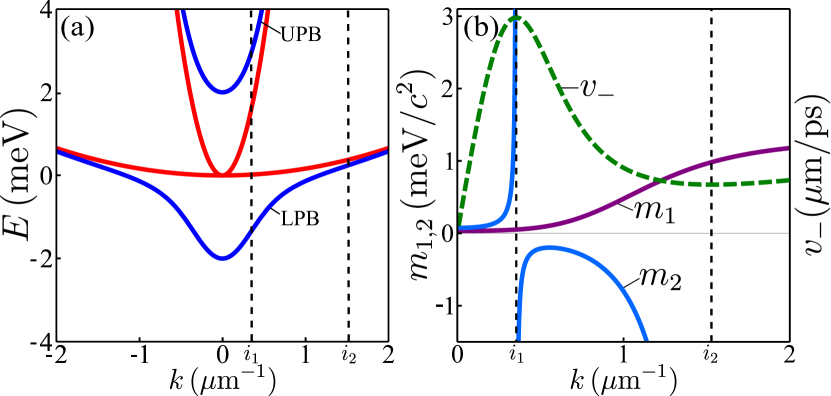
Figure 1: (Color online) a) Polariton dispersions. In red: the parabolic dispersion of the cavity photon, and the bare exciton. In blue: the polariton branches $E_{\pm}$. The vertical dashed lines at $i_{1}$ and $i_{2}$ mark the inflexion points of the LPB. b) Effective masses for the LPB as a function of momentum: in purple the inertial mass $m_{1}$, in blue the diffusive mass $m_{2}$ (negative when $i_{1}<k<i_{2}$), in green the group velocity $v_{-}$.

In this Letter, we add another member to the family of mechanisms that provide non-interacting fields with particle properties. Namely, we show that two coupled fields of different masses can support self-interfering wavepackets, resulting in the propagation of a train of sub-packets, much like the Airy beam, but without acceleration, fully-normalizable and self-created out of a Gaussian initial state. Such coupled fields can be conveniently provided in the laboratory by polaritons kavokin_book11a , the quantum superposition of the spatially extended light $\psi_{\mathrm{C}}(x,t)$ and matter fields $\psi_{\mathrm{X}}(x,t)$, cf. Fig 1. They find their most versatile and tunable implementation in semiconductors where excitons (electron-hole pairs) of a quantum well are coupled to the photons of a single-mode of a microcavity. We will consider the simplest 1D case, realized for instance in quantum wires wertz10a but similar results hold for the more common planar geometry. Since polaritons can form condensates giving rise to a wavefunction that describes their collective dynamics kasprzak06a , they are a dream laboratory to investigate the wavepacket propagation in a variety of contexts sanvitto10a , such as propagation of spin shelykh06a , bullets amo09a or Rabi oscillations liew14a with technological applications already in sight ballarini13a ; espinosa13a . Polaritons are highly valued for their nonlinear properties due to the particles self-interactions carusotto13a , illustrated by a whole family of solitons (bright, dark, composite…) egorov09a ; sich12a ; flayac11a ; christmann14a . Recently, however, also the non-interacting regime has proved to be topical, with reports of skyrmions analoguesvishnevsky13a , band structure engineering jacqmin14a focusing and conical polariton diffraction tercas14a , internal Bosonic Josephson junctions arXiv_voronova15a , emulates of oblique dark and half solitons cilibrizzi14a , $\mathbb{Z}$ topological insulator nalitov15a or the implementation of Hebbian learning in neural networks espinosa15a to name a few but illustrative examples. In most of these cases, interactions bring the physics to even farther extents rather than spoiling the underlying linear effect, that remains nevertheless the one capturing the phenomenon. The linear regime can be achieved at low densities dominici14a since the polariton interaction at the few particles level is small. In this case, the dynamics of the wavefunction $|{\psi}\rangle$ is ruled by the polariton propagator $\Pi$ such that $|{\psi(t)}\rangle=\Pi(t-t_{0})|{\psi(t_{0})}\rangle$. In free space, the propagator is diagonal in $k$ space carusotto13a :

$$\langle k^{\prime}|\Pi(t)|{k}\rangle=\exp\left[-i\begin{pmatrix}\frac{\hbar k^{2}}{2m_{\mathrm{C}}}+\Delta&\Omega_{\mathrm{R}}\\ \Omega_{\mathrm{R}}&\frac{\hbar k^{2}}{2m_{\mathrm{X}}}\\ \end{pmatrix}t\right]\delta(k-k^{\prime})$$ (1)

where $m_{\mathrm{C}}$ is the photon mass, $m_{\mathrm{X}}$ the exciton mass, $\Delta$ their detuning and $\Omega_{\mathrm{R}}$ their Rabi coupling. The eigenstates of the propagator, $\Pi(t)\left|\hskip-0.56917pt\left|k\right\rangle\hskip-1.42271pt\right\rangle_{\pm}=\exp(-iE_{\pm}t)\left|\hskip-0.56917pt\left|k\right\rangle\hskip-1.42271pt\right\rangle_{\pm}$, define both the polariton dispersion $E_{\pm}=\hbar k^{2}m_{+}+2\Delta\mp k_{\Omega}^{2}$ and the canonical polariton basis $\left|\hskip-0.56917pt\left|k\right\rangle\hskip-1.42271pt\right\rangle_{\pm}\propto(E_{\pm}(k),1)^{T}|{k}\rangle$ where $m_{\pm}=(m_{\mathrm{C}}\pm m_{\mathrm{X}})/(m_{\mathrm{C}}m_{\mathrm{X}})$ are the reduced relative masses, $k_{\Omega}=\sqrt[4]{\hbar^{2}k^{4}m_{-}^{2}-4\hbar k^{2}\Delta m_{-}+4(\Delta^{2}+4\Omega_{\mathrm{R}}^{2})}$ the dressed momentum and $|{k}\rangle$ the plane wave of well-defined momentum $k$. We use the notation $\left|\hskip-0.56917pt\left|\right\rangle\hskip-1.42271pt\right\rangle_{\pm}$ for upper ($+$) and lower ($-$) polaritons. A general polariton state is thus expressed as $\left|\hskip-0.56917pt\left|\psi\right\rangle\hskip-1.42271pt\right\rangle_{\pm}=\int_{-\infty}^{\infty}\phi_{\pm}(k)\left|\hskip-0.56917pt\left|k\right\rangle\hskip-1.42271pt\right\rangle_{\pm}\,dk$ where $\phi_{\pm}(k)$ is the scalar-field polariton wavefunction. Except for a well-defined polariton state in $k$-space, i.e., a fully delocalized polariton in real space, the photon and exciton components of a polariton cannot be jointly defined according to a given wavepacket $\phi(k)$. Indeed, except if $\phi(k)=\delta(k)$, one component gets modulated by the $E_{\pm}(k)$ factor needed to maintain the particle on its own branch. One striking consequence of this composite structure is that a polariton cannot be localized in real-space, in the sense that both its photon and exciton components be simultaneously localized. Choosing $\phi(k)$ such that either $\psi_{\mathrm{C}}(x,t=0)$ or $\psi_{\mathrm{X}}(x,t=0)$ is $\delta(x)$ results in smearing out the other component in a pointed wavefunction surrounding the singularity of the localized field, as shown in Fig. 2(a–b). Such constrains result in a rich phenomenology when involving a large enough set of momenta which, to the best of our knowledge, remained up to now safely hidden behind the simplicity of the problem. We devote the rest of the text to some of these remarkable effects, arising from the self-shaping and self-interferences of polaritons due to their composite structure, always in a non-interacting context.

It has long been known that the mass imbalance $m_{\mathrm{C}}\ll m_{\mathrm{X}}$ gives rise to a peculiar dispersion relation for the upper ($E_{+}$) and lower ($E_{-}$) polariton branches, shown in Fig. 1(a) in blue along with, in red, the parabolic dispersions of the light photon and the heavy exciton, meeting at $k=0$ ($\Delta=0$). The dynamics of a Gaussian wavepacket that is large enough in space to probe only parabolic portions of the dispersion in reciprocal space is essentially that expected from Schrödinger dynamics mark97a , diffusing with mean standard deviation of the packet size sup :

$$\sigma_{x}(t)=\sqrt{\sigma_{x}^{2}(0)+({\hbar t}/[{2m_{2}\sigma_{x}(0)}])^{2}}\,.$$ (2)

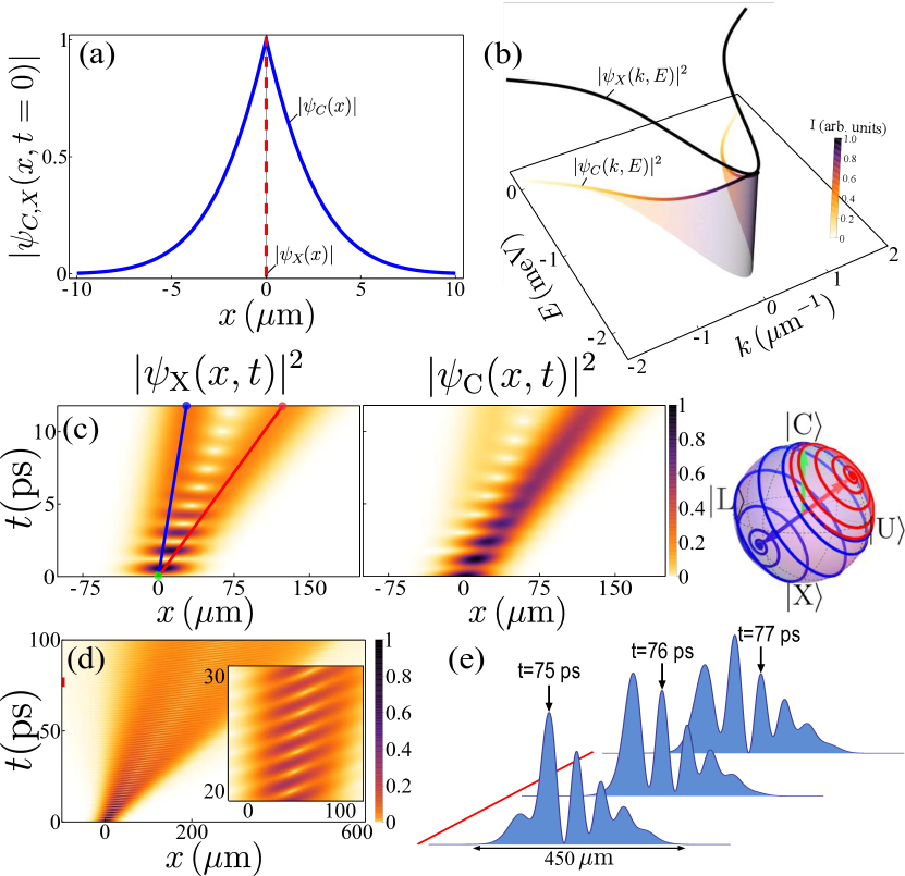
Figure 2: (a) Localizing a polariton in space is possible for one of its component only (here the one in dashed red); the other field smears out to keep the particle on its branch. (b) Counterpart of (a) in energy-momentum space with forced localization of the photon field by the delocalized exciton. (c) Spacetime evolution of $|\psi_{\textrm{C}}(x,t)|^{2}$ and $|\psi_{\textrm{X}}(x,t)|^{2}$ with as an initial condition a photon of momentum $k_{0}=$0.5\text{\,}{\mathrm{\SIUnitSymbolMicro m}}^{-1}$$. The Bloch Sphere shows the quantum state trajectories along the line of the density plot in (c). (d) Configuration with $\Delta=-\Omega_{\mathrm{R}}$, preventing splitting of the beam and resulting in ultrafast, Rabi–powered, propagating sub-packets, as shown for three snapshots of time in (e).

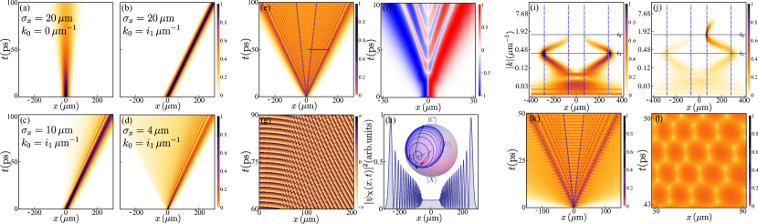
Figure 3: (Color online) (a–d) Propagation of lower polariton packets for various momenta and size, showing the emergence of the SIP for narrower packets. (e) Dynamics of an even narrower packet ($\sigma_{x}(0)=$2\text{\,}\mathrm{\SIUnitSymbolMicro m}$$ with no momentum $k_{0}=0$). (f) Current probability $j$ at early times, showing the coexistence and interleaving of net counter-propagating flows. (g) phase map in a selected region, showing $\pi$ jumps associated to each sub-peak. (h) intensity profile at $t=$90\text{\,}\mathrm{ps}$$ with the evolution of the quantum state on the Bloch sphere corresponding to the path (from green to red) plotted in (e). Wavelet decomposition of (e) at $t=$100\text{\,}\mathrm{ps}$$, and (j) in the same configuration but exciting with a momentum $k_{0}=i_{2}$. (k) Spacetime honeycomb lattice when combining the SIP with Rabi oscillations by starting with a photon as an initial condition. (l) Zoom of the hexagonal lattice.

Exciting one field only rather than eigenstate-superpositions (the polaritons) yield Rabi oscillations. Even in this simple case, there are subtleties brought by these non-parabolic dispersions. In particular, the degeneracy is lifted for some of the various concepts of masses, famously unified for the gravitational and inertial masses by Einstein as part of his theory of gravitation. For wavepackets, there are two different effective masses $m_{1}$ and $m_{2}$ larson05a , describing respectively propagation and diffusion. A wavepacket propagates with a group velocity $v_{\pm}=\partial_{k}E_{\pm}(k)$. This defines the inertial mass $m_{1}$ that determines the wavepacket velocity from de Broglie’s relation $p=\hbar k$ and the classical momentum $p=mv_{\pm}$ as:

$$m_{1}(E,k)=\hbar^{2}k(\partial_{k}E)^{-1}\,.$$ (3)

A second mass $m_{2}$, that we will call it the diffusive mass, is associated with the spreading of the wavepacket according to Eq. (2) and depends on the branch’s curvature; it reads:

$$m_{2}(E,k)=\hbar^{2}(\partial_{k}^{2}E)^{-1}\,.$$ (4)

These two masses $m_{1}$, $m_{2}$ and the packet velocity $v_{-}$ are plotted in Fig. 1(b) for the Lower Polariton Branch (LPB). Unlike parabolic dispersions, where they are equal, polariton dispersions yield qualitatively differing inertial and diffusive masses. In particular, the $k$-dependent inertial mass $m_{1}$ imposes a maximum speed for the lower polaritons sup . Beyond the inflexion point $i_{1}$, polaritons slow down if one increases their momentum (at very large $k$ the polariton becomes effectively a bare particle again with no such kinematic restriction). The coupling of the two fields with different masses results in the heavier one lagging behind the other, as seen in Fig. 2(c) for the case where a Gaussian photon wavepacket is imparted with a momentum $k=$0.5/\hbar\text{\,}\mathrm{\SIUnitSymbolMicro}\reciprocal\mathrm{m}$$, achieved experimentally by sending a pulse at an angle and overlapping both branches. This prevents the photon and exciton packets to propagate Rabi-oscillating, and instead force a splitting in two beams—the orthogonal polariton states which are eigenstates for the corresponding wavevector, as shown by their trajectory on the Bloch sphere—connected by a Rabi oscillating tunnel. The Rabi oscillations only take place when there is a spatial overlap between the polaritons. The two propagating packets maintain their coherence despite their space separation and would Rabi oscillate if meeting again, due, for instance, to a ping-pong reflection anton13a . The splitting in two beams can be minimized by tuning parameters to equalize the polaritons masses, in particular the inertial ones. Combined with the bending of the Rabi oscillations in spacetime, which can be achieved at nonzero detuning, this leads to propagation of Rabi oscillations, that produce ultrafast subpackets moving inside a mother packet, as shown in Fig. 2(d) and for three snapshots in time in (e). The subpackets, continuously formed in the tail of the mother packet, propagate inside one order of magnitude faster, powered by Rabi oscillations, before dying in the head. Each sub-peak acquires properties of an identifiable object that can be tracked in time. The full dynamics is available in an accompanying video sup . Now on the diffusive mass $m_{2}$: it diverges at the two inflexion points $i_{1,2}$ of the LPB and is negative in between. Exciting at the inflexion points thus cancels diffusion of the wavepacket as seen in Eq. (2) and in Fig. 3(a,b) with the propagation of a broad ($\sigma_{x}(0)=$20\text{\,}\mathrm{\SIUnitSymbolMicro m}$$) lower-polariton wavepacket with an imparted momentum of (a) $k_{0}=0$ and (b) $k_{0}=i_{1}$. The excitation around the inflexion point has already been used to generate bright solitons and soliton trains egorov09a ; egorov10a ; sich12a ; sich14a . In these cases, the soliton mechanism is the conventional interplay between negative effective mass and repulsive nonlinear interactions. The role of the high effective mass close to the inflexion point, which cancels the diffusion, was not however fully estimated.

The interesting phenomenology discussed so far illustrates isolated features of the polariton propagation. A new physical picture emerges when combining several aspects within the same wavefunction, leading to the concept of self-interfering packets (SIP). This is obtained when reducing the size of the wavepacket in real space, that is, increasing the staggering on the dispersion in momentum-space ($\sigma_{k}(0)=1/\sigma_{x}(0)$), to an extent enough to probe polaritonic deviation from the parabolic dispersion. In this case, the negative mass plays an explicit role. Negative masses are a recurrent theme in physics but this is typically meant for the inertial mass wimmer13a . The sign of the diffusive mass would seem, at first, not to play a role since it enters as a square in Eq. (2), and this is indeed the case for a regular packet with momentum $i_{1}<k<i_{2}$. When straddling over the divergence, however, self-interferences occur between harmonics of the packet subject to the positive mass and others to the negative mass. This result in a complete reshaping of the wavefunction, as shown in Fig. 3(c,d) decreasing $\sigma_{x}(0)$ down to $10\text{\,}\mathrm{\SIUnitSymbolMicro m}$ and $4\text{\,}\mathrm{\SIUnitSymbolMicro m}$. The part of the packet that goes beyond the divergence is reflected back and interferes with the rest of the packet that still propatages forward, resulting in ripples. Reducing the packet to $\sigma_{x}(0)=$2\text{\,}\mathrm{\SIUnitSymbolMicro m}$$ produces the striking pattern seen in Fig. 3(e), without even the need of an imparted momentum. While for a parabolic dispersion, squeezing the packet in space merely causes a faster diffusion, in the polariton case, there is thus a critical diffusion beyond which the packet stops expanding and folds back onto itself. Since this happens when the wavefunction encounters the inflection point of the polariton dispersion, there is a “mass wall” against which the packet bounces back. If the dispersion also features another inflection point at larger $k$, which can be the case for small enough exciton masses, this reflection happens again, this time resulting in a shielding from this self-interference of the core of the mother packet, as shown on the cut in intensity Fig. 3(h) (the diffusion cones are the solution of $\partial_{k}^{2}E_{-}=0$, cf. Fig. 3(e)). More importantly from a conceptual point of view, as a result of this coexistence of masses of opposite signs within the same packet, the mother wavepacket $|{\psi}\rangle$ fragments itself into two trains of daughter shape-preserving subpackets which travel in opposite directions. The overall momentum $\langle\psi|p|{\psi}\rangle=0$ is null but the self-shaping of the wavefunction redistributes it through its subpackets as a series of nonzero momenta. Each sub-peak can be identified by as a polariton as seen by following its quantum state on the Bloch sphere, that lies onto the meridian between $|{\mathrm{L}}\rangle$ and $|{\mathrm{X}}\rangle$, as shown in Fig. 3(f) following a path (at $t=$50\text{\,}\mathrm{ps}$$) from the central aera—shielded from the self-interferences—to the edge of the packet. The SIP can therefore be seen as a train of successive polariton packets, “emitted” by the area shielded from the self-interference at the rate of Rabi oscillations, and that retain their individuality as they propagate inside the mother packet. The full quantum state dynamics along these paths can also be seen vividly in a supplementary video sup . Successive peaks furthermore feature a maximal phase shift of $\pi$ in the phase $\phi(x,t)$ of the total wavefunction $\psi(x,t)=|\psi(x,t)|\exp(i\phi(x,t))$, as shown in Fig. 3(g). Baring the fact that they do not involve self-interactions to account for their cohesion and other properties making them particles lookalike, these propagating subpackets behave in many respects as soliton-like objects. The analogy with Airy beams is conspicuous.

One can gain additional insights into the nature of the SIP through the current probability $j=i\hbar/2m_{1}(\psi^{\ast}\partial_{x}\psi-\psi\partial_{x}\psi^{\ast})$, in Fig. 3(f) where the packet is plainly seen to alternate backward and forward net flows. More sophisticatedly, considering the wavelet transform (WT) debnath_book15a $\mathbb{W}_{a,b}(\psi)=\frac{1}{\sqrt{|a|}}\int_{-\infty}^{+\infty}\psi(x)\mathscr{G}^{\ast}\left(\frac{x-b}{a}\right)\,\mathrm{d}x$, in our case, of the Gabor wavelet family $\mathscr{G}(z)=\sqrt[4]{\pi}\exp(i\omega x)\exp(-x^{2}/2)$, allows us to decompose the wavefunction into Gaussian packets, which are the basic packets as far as propagation and diffusion are concerned. Such an extension of the Fourier transform is common in signal processing but has found so far little echo to study the dynamics of wavepackets baker12a . We show in Fig. 3(i) the energy density $|\mathbb{W}_{k,x}|^{2}$ of the wavefunction in the $(x-k)$ plane at $t=100\mathrm{ps}$. One can see clearly how the self-interferences force the polariton packet to remain within the diffusion cone (blue dashed lines), by diverting the flow backward, (i) one or (j) two times when the second inflexion point ($k_{0}=i_{2}$) is reached. Other fundamental connections could be established. For instance, patterns strikingly similar to Fig. (3(e)) were observed in the quenched dynamics of a quantum spin chains with magnons liu14b , a completely different system. This suggests that coupled light-fields feature fundamental and universal dynamical evolutions. Combining this characteristic pattern with that of Rabi oscillations leads to the space-time propagation presented in Fig. 3(c). The protected area simply exhibits Rabi oscillations. The outer area is propagating upper polaritons and is not affected either by oscillations nor interferences. In the SIP area, however, sitting between the two mass walls, the interplay of Rabi oscillations and self-interferences produces and hexagonal lattice. Here, instead of the emergence of propagating particles, a spacetime crystal is formed with the manifest ordering of the previously freely propagating train of polaritons. This striking structure is, again, sculpted self-consistently out of a simple Gaussian state by the dynamics of coupled non-interacting fields.

In conclusion, we have shown the intricate wavepacket propagations of coupled fields (polaritons). While the boundless diffusion of a Schrödinger wavepacket in a parabolic dispersion ultimately leads to complete indeterminacy, the polariton case can sustain traceable objects with always well-defined properties, such as their shape, position, momentum and quantum state. This gives rise to a concept of particles similar to that brought by the soliton in nonlinear media or Airy beams in non-interacting ones. While these are formed by self-interaction and phase-shaping, the individuality of polaritons is acquired and maintained through self-interferences powered by the Rabi coupling. This shows that even in the linear regime, the polariton dynamics is rich and able to produce intricate structures out of mere Gaussian initial states. This could lead to applications, by imparting momentum powered by the Rabi oscillations or in the limit of few particles, for quantum computing, by a proper wiring and directing of the sub-packets, since all this happens in a strict linear regime.

Acknowledgments: This work is funded by the “POLAFLOW” ERC Starting Grant. We thank L. Dominici, D. Ballarini, E. del Valle and D. Sanvitto for discussions.

Self-interfering wavepackets

Supplementary Material

 

I Introduction and Outlook

The theoretical model describing self-interacting wavepackets (SIP) is simple: two coupled 1D Schrödinger equations in the linear regime (see section IV for the 2D case). The simplicity of the equation is no guarantee that its extent and depth are rapidly exhausted, as illustrated by the Schrödinger equation, one of the most fundamental equation of modern physics, for which the self-accelerating solution was discovered only in 1979. There should be hope, however, that some closed-form solutions are available. In Section III we show that the SIP, if it has such analytical expressions, does not seem to be reducible to a simple closed form. We could express it as a complex combinatorial superposition of Bessel functions, as could be expected from propagating packets, weighted by polaritonic factors, such as the dressed momentum $k_{\Omega}$. Before discussing this structure, we start in Section II with more details on the exact solutions, both from the formalism and numerical simulations point of view, contrasting in particular the multitude of ways that one has to poke at the polariton wavefunction. Last Section, V, gives an overview of the rest of the Supplementary material, that consists of animated movies that illustrate, maybe better than equations, the mesmerizing dynamics of polaritons.

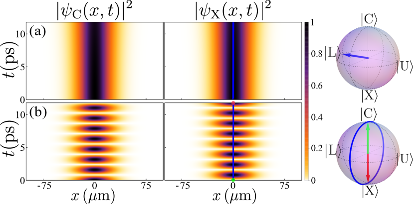
Figure 4: (Color online) Polariton propagation of delocalized wavepackets, as seen through the photonic ($\psi_{\mathrm{C}}$) and excitonic ($\psi_{\mathrm{X}}$) components for the cases of (a) upper row: a lower polariton at $t=0$ and (b) lower row: a photon. The diffusion is negligible over the selected time window and the staggering on the dispersion too small to evidence polariton self-interference effects. Parameters: $\Omega_{\mathrm{R}}=2\,\textrm{meV}\,,m_{\mathrm{C}}=0.025\,\textrm{meV}\,\textrm{ps}^{2}\,\mu\textrm{m}^{-2},m_{\mathrm{X}}=0.2\,\textrm{meV}\,\textrm{ps}^{2}\,\mu\textrm{m}^{-2}\,,\sigma_{x}=$20\text{\,}\mathrm{\SIUnitSymbolMicro m}$$.

II More polariton propagation

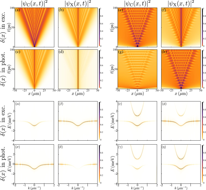
Figure 5: (Color online) Propagation of sharp packets. As seen in both real-space as a function of time (upper two rows) and through their dispersion (energy as a function of momentum, lower two rows) through the light emitted by the cavity (C) or through the direct exciton emission (X) for the cases of a lower polariton propagation (two columns on the left) and of a bare state propagation (two columns on the rigth). In the case of polaritons, (a–d), the exciton (upper row) or the photon (lower row) is perfectly localized at $t=0$ with the other component defined such that the the particle remains on its branch. In the case of bare particles (e–h), the initial state is simply a photon (upper row) or an exciton (lower row) with the other component empty at $t=0$. Greek-numbered panels correspond to the latin-numbered ones. Parameters: $\Omega_{\mathrm{R}}=0.5\,\textrm{meV},m_{\mathrm{C}}=0.5\,\textrm{meV}\,\textrm{ps}^{2}\,\mu\textrm{m}^{-2}$.

The polariton propagator, Eq. (1) of the main text is easily found in $k$ space (we work here with $\Delta=0$):

$$\langle k^{\prime}|\Pi|{k}\rangle=\begin{pmatrix}\exp(\frac{-ik^{2}m_{+}t}{4})\left(\cos(\frac{k_{\Omega}^{2}t}{4})+i\frac{k^{2}}{k_{\Omega}^{2}}m_{-}\sin(\frac{k_{\Omega}^{2}t}{4})\right)&-\frac{i4\Omega_{\mathrm{R}}}{k_{\Omega}^{2}}\exp(\frac{-ik^{2}m_{+}t}{4})\sin(\frac{k_{\omega}^{2}t}{4})\\ -\frac{i4\Omega_{\mathrm{R}}}{k_{\Omega}^{2}}\exp(\frac{-ik^{2}m_{+}t}{4})\sin(\frac{k_{\omega}^{2}t}{4})&\exp(\frac{-ik^{2}m_{+}t}{4})\left(\cos(\frac{k_{\Omega}^{2}t}{4})-i\frac{k^{2}}{k_{\Omega}^{2}}m_{-}\sin(\frac{k_{\Omega}^{2}t}{4})\right)\\ \end{pmatrix}\delta(k-k^{\prime})\,,$$ (S1)

where we remind the important dressed momentum variable $k_{\Omega}$:

$$k_{\Omega}\equiv\sqrt[4]{k^{4}m_{-}^{2}+16m_{+}^{2}\Omega_{\mathrm{R}}^{2}}\,,$$ (S2)

with $m_{\pm}=(m_{\mathrm{C}}\pm m_{\mathrm{X}})/(m_{\mathrm{C}}m_{\mathrm{X}})$ (note again that $k_{\Omega}$ is a function of $k$). We also assume $\hbar=1$. Polaritons are maybe best formally defined as the states with a well-defined momentum and, consequently, also energy. They satisfy:

$$\Pi(t)\left|\hskip-0.56917pt\left|k\right\rangle\hskip-1.42271pt\right\rangle_{\pm}=\exp(-iE_{\pm}t)\left|\hskip-0.56917pt\left|k\right\rangle\hskip-1.42271pt\right\rangle_{\pm}\,,$$ (S3)

and as such are expressed as:

$$\left|\hskip-0.56917pt\left|k\right\rangle\hskip-1.42271pt\right\rangle_{\pm}\propto\begin{pmatrix}E_{\pm}(k)\\ 1\end{pmatrix}|{k}\rangle\,,$$ (S4)

for $+$ (resp. $-$) the upper (resp. lower) polariton, with $E_{\pm}$ the pivotal polariton quantity, the dispersion:

$$E_{\pm}=k^{2}m_{+}\mp k_{\Omega}^{2}\,.$$ (S5)

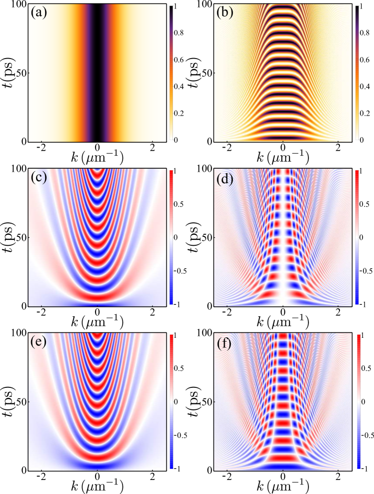
Figure 6: (Color online) Propagation in $k$-space for non-diffusing packets of, left column, a lower polariton and, right column, a photon, as seen through, from up to bottom: $|\psi_{\mathrm{C}}(k,t)|^{2}$, $\Re(\psi_{\mathrm{C}}(k,t))$ and $\Im(\psi_{\mathrm{C}}(k,t))$. Parameters: $\Omega_{\mathrm{R}}=0.5\,\textrm{meV},m_{\mathrm{C}}=0.5\,\textrm{meV}\,\textrm{ps}^{2}\,\mu\textrm{m}^{-2}$.

States (S4) form a canonical basis out of which a general polariton state is obtained by linear combination:

$$\left|\hskip-0.56917pt\left|\psi\right\rangle\hskip-1.42271pt\right\rangle_{\pm}=\int_{-\infty}^{\infty}\phi_{\pm}(k)\left|\hskip-0.56917pt\left|k\right\rangle\hskip-1.42271pt\right\rangle_{\pm}\,dk\,,$$ (S6)

with $\phi_{\pm}(k)$ the scalar-field (upper/lower) polariton wavefunction. All the results in this text follow from the impossibility to evolve such a general polariton state in time with the complex rotation of free propagation as in Eq. (S3), due to its two-component character. We have already discussed in the main text some important constrains of such a structure: for instance, that except for a well-defined polariton state in $k$-space, i.e., a completely delocalized polariton in real space, the photon and exciton components of a polariton cannot be jointly defined according to a given wavepacket $\phi(k)$, e.g., a Gaussian packet, since one component gets modulated by the $E_{\pm}$ factor needed to maintain the particle on its branch. Gaussian packets for both the photon and the exciton result in populating both polariton branches. The general case obviously admixes the two types of polaritons: $|{\psi}\rangle=\sum_{\sigma=\pm}\int\phi_{\sigma}(k)\left|\hskip-0.56917pt\left|k\right\rangle\hskip-1.42271pt\right\rangle_{\pm}\,dk$. These results that impose strong constrains on a polariton wavepacket must be contrasted with the conventional picture one has of the polariton as a particle, which is that of states $\left|\hskip-0.56917pt\left|k\right\rangle\hskip-1.42271pt\right\rangle_{\pm}$ and is, in good approximation, recovered for large enough packets as shown in Fig. 4. The particle is here broad enough in space to have a small diffusion, cf. Eq. (2), and Rabi oscillations may be present depending on the state preparation, which however do not result in qualitative novelties. The situation is completely different when considering overlaps in $k$ space, that is, sharp packets in real spaces. The propagation of such sharp packets is shown in Fig. 5 for various initial conditions: as a lower polariton (left part of the figure) or as a bare particle (exciton or photon, right part of the figure) and such that the excitonic component is perflectly localized at $t=0$ (upper row) or the photon component is (lower row). The wavepacket evolution is also shown as seen either through its photon or exciton field. Experimentally, the photon field is typically the one observed by recording the light leaked by the cavity. One sees variations around the themes exposed in the main text, with more or less pronounced features in some of the configurations. The clearest effects are obtained for confined excitons and observation through the cavity is always a good vantage point. For each case of propagation in space-time, we also show in Fig. 5($\alpha$–$\eta$) the corresponding dispersion, which is the double Fourier transform. This shows how, indeed, the lower polariton only populates its own branch. It also provides an alternative view of the various localized states, e.g., the localized photon does not populate the photon-like part of the polariton branch in the exciton spectrum (panel $\delta$) and vice-versa with the localized exciton in the photon spectrum (panel $\alpha$).

We now proceed with the underlying Mathematical expressions. For, say, the lower polariton case prepared so that the photon component is perfectly localized at $t=0$ (in the case where, for concision in the notation, we assume from now on $m_{\mathrm{X}}\rightarrow\infty$), we find from Eqs. (S1–S6):

$$\psi_{\mathrm{C}}(k,t) = \exp\left(-i\frac{k^{2}-k^{2}_{\Omega}}{4m_{\mathrm{C}}}t\right)\frac{k^{2}_{\Omega}-k^{2}}{4\Omega_{\mathrm{R}}m_{\mathrm{C}}}\,,$$ (S7a)

$$\psi_{\mathrm{X}}(k,t) = \exp\left(-i\frac{k^{2}-k^{2}_{\Omega}}{4m_{\mathrm{C}}}t\right)\,.$$ (S7b)

The result is extremely simple in this picture (time–momentum). There is no time dynamics for the density $|\psi_{\mathrm{X},\mathrm{C}}|^{2}$: the perfectly localized exciton at $t=0$ results in a completely delocalized wavefunction at all times $|\psi_{\mathrm{X}}|^{2}=1$. The corresponding photon wavefunction is qualitatively similar to a Voigt lineshape in $k$-space, which we will use in next Section to derive approximated expressions. It is shown on the left column of Fig. 6. In all cases, however, there is of course a dynamics of the wavefunction itself, as seen through its real and imaginary parts on the figure. There is a slowing down of the oscillations with increasing $|k|$. The Fourier-transform in $k$ of this pattern gives the spacetime propagation in Fig. 5(a).

The case of only the perfectly localized exciton as the initial condition (i.e., in the photon vacuum rather than the field needed to provide a lower polariton), i.e., $\psi_{-}(x,t=0)=(\delta(x),0)^{T}$, is given directly by the columns of Eq. (S1):

$$\psi_{\mathrm{C}}(k,t) = \exp\left(-\frac{ik^{2}t}{4m_{\mathrm{C}}}\right)\left[\cos\left(\frac{k_{\Omega}^{2}t}{4m_{\mathrm{C}}}\right)-i\left(\frac{k}{k_{\Omega}}\right)^{2}\sin\left(\frac{k_{\Omega}^{2}t}{4m_{\mathrm{C}}}\right)\right]\,,$$ (S8a)

$$\psi_{\mathrm{X}}(k,t) = \exp\left(-\frac{ik^{2}t}{4m_{\mathrm{C}}}\right)(-i\Omega_{\mathrm{R}}t)\operatorname{sinc}\left(\frac{k_{\Omega}^{2}t}{4m_{\mathrm{C}}}\right)\,.$$ (S8b)

The corresponding propagation in momentum-space is shown on the right column of Fig. 6. There is, this time, a dynamic in the density, namely, the Rabi oscillations, with, in contrast to dynamics of the real an imaginary parts, a speeding up of the oscillations with increasing $|k|$, corresponding to the effective Rabi frequency of effectively detuned exciton-photon coupled states. The Fourier-transform in $k$ of this pattern gives the spacetime propagation in Fig. 5(e).

We have also discussed in the main text how a polariton wavepacket propagates with a group velocity $v_{\pm}=\partial_{k}E_{\pm}(k)$ that, for the lower polariton, features a local maximum. It reads:

$$v_{-}=\frac{k}{2m_{+}}-\frac{\frac{\Delta}{k}-\frac{k}{2m_{-}}}{\sqrt{1-\frac{4m_{-}\Delta}{k^{2}}+\frac{4m_{-}^{2}(4\Omega_{\mathrm{R}}^{2}+\Delta^{2})}{k^{4}}}}\,,$$ (S9)

which is shown on Fig. 7 in blue. The local maximum is obtained at the first inflexion point of the dispersion, $k=i_{1}$, where the polaritons also do not diffuse. Increasing the momentum makes the particle heavier and actually reduces its speed. A local minimum is attained at the second inflexion point, $k=i_{2}$, where the polariton also propagate without diffusion but now with a low speed. At larger $k$, Eq. (S9) becomes linear and tends to the speed of the bare exciton, as indeed for $k\gg 0$, $v_{-}(k)\to k/m_{\mathrm{X}}$, cf. Fig. 7 in dashed red for a non detuned system. If there is no second inflexion point (for an infinitely heavy exciton mass), there is an absolute maximum speed for the polaritons since the bare exciton group velocity vanishes (green curve).

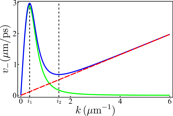
Figure 7: (Color online) Speed of the lower polariton as a function of its imparted momentum: there is a maximum speed for lower polaritons. Larger momenta result in slower particles. Local maxima are given by the inflexion points. At large enough $k$, the polariton becomes exciton-like and suffers no such restriction. If the exciton mass is infinite, polaritons have an absolute maximum velocity.

III Approximations

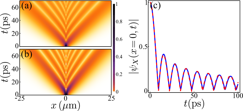
Figure 8: (Color online) (a,b) $|\psi_{\mathrm{X}}(x,t)|^{2}$ calculated from the exact result Eq. (S7b) and the approximated one, Eq. (S11). (c) Normalized intensity at the center of the wavepacket ($x=0$): exact result through the Fourier Transform of Eq. (S7b) (blue line) and the analytical expression Eq.S12 (red dashed line). The approximation appears to be exact at $x=0$.

We could not find manageable closed form expressions for the Fourier Transform of the term $\exp(k_{\Omega}^{2}-k^{2})$ that capture the (lower) polaritonic self-interference effect. The term $k^{2}-k_{\Omega}^{2}$ for the (lower) polariton momentum distribution can however be well approximated by a Voigt distribution, since it combines both exponential and fat-tail types of decay. Since the fat-tail is expected to play a dominant role qualitatively, we assume simply a Lorentzian distribution $f(k)={4\Omega_{\mathrm{R}}m_{\mathrm{C}}}/\big{(}1+\frac{k^{2}}{4\Omega_{\mathrm{R}}m_{\mathrm{C}}}\big{)}$, thus approximating Eq. (S7b) by:

$$\psi_{\mathrm{X}}(k,t)\simeq\frac{-\exp{\frac{it\Omega_{\mathrm{R}}}{1+k^{2}/(4m_{\mathrm{C}}\Omega_{\mathrm{R}})}}}{1+k^{2}/(4m_{\mathrm{C}}\Omega_{\mathrm{R}})}\,,$$ (S10)

which Fourier Transform can be obtained by a series expansion of the exponential, providing the real-space dynamics of the SIP:

$$\psi_{\mathrm{X}}(x,t)\simeq\\ \sum_{n=0}^{\infty}\frac{-4\sqrt{\pi}(m_{\mathrm{C}}\Omega_{\mathrm{R}})^{\frac{3+2n}{4}}(it\Omega_{\mathrm{R}})^{n}|x|^{\frac{1}{2}+n}K_{\alpha}(2\sqrt{\Omega_{\mathrm{R}}m_{\mathrm{C}}}|x|)}{n!^{2}}\,,$$ (S11)

where $K_{\alpha}(z)$ is the modified Bessel functions (solution of th equation $z^{2}y^{\prime\prime}+zy^{\prime}-(z^{2}+n^{2})y=0$) and with $\alpha=n+1/2$. The propagation of the wavepacket calculated numerically with the Fourier Transform (a) and the one obtain with the analytical formula in Eq. S11 (b) are compared in Fig. 8. There is a good qualitative agreement, with only the size of the propagation cone differing slightly, due to the width difference between the Lorentzian distribution and the actual one. One can therefore trust the approximation to give some insights into the nature of the SIP. First, the SIP is indeed a phenomenon of many interferences. The convergence of the series is obtained for a number of terms in the sum that increases linearly with time $t$, showing how each new peak arises from an added term and thus a next order in the interference. Also, at the center of the wavepacket ($x=0$), the previous expression can be reduced to a simple form:

$$\psi_{\mathrm{X}}(x=0,t)\simeq-2\pi\sqrt{\Omega_{\mathrm{R}}m_{\mathrm{C}}}\operatorname{e}^{\frac{it\Omega_{\mathrm{R}}}{2}}J_{0}\left(\frac{t\Omega_{\mathrm{R}}}{2}\right)\,,\\$$ (S12)

where $J_{n}(z)$ is the Bessel function of the first kind. Since the departure between Eq. (S11) and the exact numerical solution is mainly due to the extent of the envelope of the momentum, one can expect a better agreement at $x=0$, and indeed we find that there is a perfect match, as seen in Fig. 8(c). Equation (S12) confirms that the successive peaks that shape the SIP appear at the Rabi frequency $\Omega_{\mathrm{R}}$. The photon mass $m_{\mathrm{C}}$ (we remind that we assumed here an infinite exciton mass) acts only on the intensity. In the same way, one can obtain the corresponding series for the photon field:

$$\psi_{\mathrm{C}}(x,t)\simeq\\ \sum_{n=0}^{\infty}\frac{4\sqrt{\pi}(m_{\mathrm{C}}\Omega_{\mathrm{R}})^{\frac{2n+1}{4}}(it\Omega_{\mathrm{R}})^{n}|x|^{n-\frac{1}{2}}K_{\beta}(2\sqrt{\Omega_{\mathrm{R}}m_{\mathrm{C}}}|x|)}{n!\Gamma(n)}\,,$$ (S13)

with $\beta=n-1/2$, showing how both structures are tightly related and the sort of complexity that describes them. Series for photons or excitons as initial conditions can also be obtained from Eq. S8a and S8b, involving Hypergeometric functions which, however, are too cumbersome to be written here.

IV SIP in two dimensions

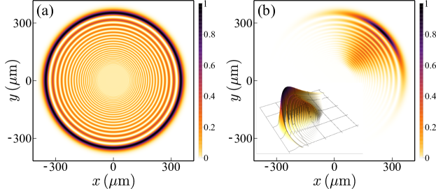
Figure 9: (Color online) SIP in two-dimensions. (a) With full radial symmetry when self-interfering in all directions. A central disk is shielded from interference just like in the 1D case and feature a flat plateau of lower polaritons. (b) When imparted with momentum, the packet self-interfere in the direction of its propagation and diffuses radially. Parameters : $\Omega_{\mathrm{R}}=2\,\textrm{meV}\,,m_{\mathrm{C}}=0.025\,\textrm{meV}\,\textrm{ps}^{2}\,\mu\textrm{m}^{-2},m_{\mathrm{X}}=0.2\,\textrm{meV}\,\textrm{ps}^{2}\,\mu\textrm{m}^{-2},$ (a) $\sigma_{x}=$2\text{\,}\mathrm{\SIUnitSymbolMicro m}$$, (b) $\sigma_{x}=$4\text{\,}\mathrm{\SIUnitSymbolMicro m}$,\,k_{x}=k_{y}=i_{1}$.

So far, we have considered 1D cases, which are indeed possible in heterostructures by confining in the two other dimensions (quantum wires). Polariton propagation is however popular in the 2D geometry as well and we quickly discuss what happens in this configuration. Since the system is linear and uncoupled in transverse coordinates, the dynamics follows trivially from the previous results and symmetry. With a full radial symmetry, all the phenomenology is conserved in 2D, with rotational invariance. This is shown in Fig. 9(a) where the propagation of a SIP is shown after $100\text{\,}\mathrm{ps}$, after preparing a narrow Gaussian wavepacket at $t=0$ (and at the origin of the plane). This is the counterpart of the case of Fig. 3(e) of the main text. The propagation and thus the shape of the wavepacket are similarly determined by the dispersion and the way it is excited. There is also, depending on the proximity of the second inflection point, a central area shielded from the interferences, which is now a disk, whose diameter is also determined by a zero of $\partial_{k}^{2}E_{-}=0$. Also, like in the 1D case, one can impulse the propagation of the packet in a desired direction by imparting a momentum. This is shown in Fig. 9(b) with the propagation of a smaller wavepacket when exciting the dispersion at the first inflexion point ($k_{x}=k_{y}=i_{1}$). By using squeezed Gaussian packets, one can propagate a SIP with fronts that remain parallel and orthogonal to the direction of motion.

V Movies

We also provide two movies that illustrate vividly the polariton dynamics.

The movie I-QuantumState.avi animates Fig.3 (e,h) of the main text. It shows how a narrowly squeezed lower polariton wavepacket self-interferes and produces, as a result, two trains of sub-packets propagating back to back, emerging from a polariton sea shielded from the interferences. To show how the overall structure of the SIP is connected to the individual identity of each packet, we also present dynamically on the Bloch sphere the evolution of the quantum state on a path that links the center of the wavepacket to the side of the diffusion cone (from the green to the red point on the density plot, mached with the green and red arrows on the sphere). The state in the central area—shielded from interferences—is the lower polariton. In the interferences zone, crossing a fringe induces a loop on the sphere that crosses the meridian of states $|{\mathrm{C}}\rangle$–$|{\mathrm{L}}\rangle$–$|{\mathrm{X}}\rangle$. Each peak converges in time towards a well defined polariton state on the meridian.

The movie II-PolaritonRiffle.avi animates the case of Fig. 2(d,e) of the main text. It shows the propagation of a photon wavepacket (at $t=0$) with a momentum and negative detuning. A judicious choice of parameters permits to maintain a spatial overlap between the two polaritons, conserving the Rabi oscillations which, due to the detuning, are bent in spacetime (see main text). This results in the propagation of ultrafast subpackets within the mother packet. This is well seen on the animation after $35\text{\,}\mathrm{ps}$ of animation time, which is the time needed for the packet to develop the structure (the initial condition is a Gaussian packet).

References

- (1) Ng, T.-K. Introduction to Classical and Quantum Field Theory (Wiley, 2009).
- (2) Schrödinger, E. Der stetige übergang von der Mikro- zur Makromechanik. Naturwissenschaften 14, 664 (1926).
- (3) Korteweg, D. J. & de Vries, G. On the change of form of long waves advancing in a rectangular canal, and on a new type of long stationary waves. Phil. Mag. 39, 422 (1895).
- (4) Berry, M. V. & Balazs, N. L. Nonspreading wave packets. Am. J. Phys. 47, 264 (1979).
- (5) Broky, J., Siviloglou, G. A., Dogariu, A. & Christodoulides, D. N. Self-healing properties of optical Airy beams. Opt. Lett. 16, 12880 (2008).
- (6) Siviloglou, G. A., Broky, J., Dogariu, A. & Christodoulides, D. N. Observation of accelerating Airy beams. Phys. Rev. Lett. 99, 213901 (2007).
- (7) Voloch-Bloch, N., Lereah, Y., Lilach, Y., Gover, A. & Arie, A. Generation of electron Airy beams. Nature 494, 331 (2013).
- (8) Zhang, P. et al. Nonparaxial Mathieu and Weber accelerating beams. Phys. Rev. Lett. 109, 193901 (2012).
- (9) Kavokin, A., Baumberg, J. J., Malpuech, G. & Laussy, F. P. Microcavities (Oxford University Press, 2011), 2 edn.
- (10) Wertz, E. et al. Spontaneous formation and optical manipulation of extended polariton condensates. Nat. Phys. 6, 860 (2010).
- (11) Kasprzak, J. et al. Bose–Einstein condensation of exciton polaritons. Nature 443, 409 (2006).
- (12) Sanvitto, D. et al. Polariton condensates put in motion. Nanotechnology 21, 134025 (2010).
- (13) Shelykh, I. A., Rubo, Y. G., Malpuech, G., Solnyshkov, D. D. & Kavokin, A. Polarization and propagation of polariton condensates. Phys. Rev. Lett. 97, 066402 (2006).
- (14) Amo, A. et al. Collective fluid dynamics of a polariton condensate in a semiconductor microcavity. Nature 457, 291 (2009).
- (15) Liew, T., Rubo, Y. & Kavokin, A. Exciton-polariton oscillations in real space. Phys. Rev. A 90, 245309 (2014).
- (16) Ballarini, D. et al. All-optical polariton transistor. Nat. Comm. 4, 1778 (2013).
- (17) Espinosa-Ortega, T. & Liew, T. C. H. Complete architecture of integrated photonic circuits based on and and not logic gates of exciton polaritons in semiconductor microcavities. Phys. Rev. B 87, 195305 (2013).
- (18) Carusotto, I. & Ciuti, C. Quantum fluids of light. Rev. Mod. Phys. 85, 299 (2013).
- (19) Egorov, O. A., Skryabin, D. V., Yulin, A. V. & Lederer, F. Bright cavity polariton solitons. Phys. Rev. Lett. 102, 153904 (2009).
- (20) Sich, M. et al. Observation of bright polariton solitons in a semiconductor microcavity. Nat. Photon. 6, 50 (2012).
- (21) Flayac, H., Solnyshkov, D. D. & Malpuech, G. Oblique half-solitons and their generation in exciton-polariton condensates. Phys. Rev. B 83, 193305 (2011).
- (22) Christmann, G. et al. Oscillatory solitons and time-resolved phase locking of two polariton condensates. New J. Phys. 16, 103039 (2014).
- (23) Vishnevsky, D. V. et al. Skyrmion formation and optical spin-Hall effect in an expanding coherent cloud of indirect excitons. Phys. Rev. Lett. 110, 246404 (2013).
- (24) Jacqmin, T. et al. Direct observation of Dirac cones and a flatband in a honeycomb lattice for polaritons. Phys. Rev. Lett. 112, 116402 (2014).
- (25) Terças, H., Flayac, H., Solnyshkov, D. & Malpuech, G. Non-Abelian gauge fields in photonic cavities and photonic superfluids. Phys. Rev. Lett. 112, 066402 (2014).
- (26) Voronova, N., Elistratov, A. & Lozovik, Y. Detuning-controlled internal oscillations in an exciton-polariton condensate. arXiv:1503.04231 (2015).
- (27) Cilibrizzi, P. et al. Linear wave dynamics explains observations attributed to dark solitons in a polariton quantum fluid. Phys. Rev. Lett. 113, 103901 (2014).
- (28) Nalitov, A., Solnyshkov, D. & Malpuech, G. Polariton topological insulator. Phys. Rev. Lett. 114, 116401 (2015).
- (29) Espinosa-Ortega, T. & Liew, T. Perceptrons with Hebbian learning based on wave ensembles in spatially patterned potentials. Phys. Rev. Lett. 114, 118101 (2015).
- (30) Dominici, L. et al. Ultrafast control and Rabi oscillations of polaritons. Phys. Rev. Lett. 113, 226401 (2014).
- (31) Márk, G. I. Analysis of the spreading Gaussian wavepacket. Eur. Phys. J. B 18, 247 (1997).
- (32) See Supplementary Material.
- (33) Larson, J., Salo, J. & Stenholm, S. Effective mass in cavity QED. Phys. Rev. A 72, 013814 (2005).
- (34) Antón, C. et al. Quantum reflections and shunting of polariton condensate wave trains: Implementation of a logic AND gate. Phys. Rev. B 88, 245307 (2013).
- (35) Egorov, O., Gorbach, A., Lederer, F. & Skryabin, D. Two-dimensional localization of exciton polaritons in microcavities. Phys. Rev. Lett. 105, 073903 (2010).
- (36) Sich, M. et al. Effects of spin-dependent interactions on polarization of bright polariton solitons. Phys. Rev. Lett. 112, 046403 (2014).
- (37) Wimmer, M. et al. Optical diametric drive acceleration through action–reaction symmetry breaking. Nat. Phys. 9, 780 (2013).
- (38) Debnath, L. & Shah, F. A. Wavelet Transforms and Their Applications (Birkhăuser, 2015), 2 edn.
- (39) Baker, C. H., Jordan, D. A. & Norris, P. M. Application of the wavelet transform to nanoscale thermal transport. Phys. Rev. B 86, 104306 (2012).
- (40) Liu, W. & Andrei, N. Quench dynamics of the anisotropic heisenberg model. Phys. Rev. Lett. 112, 257204 (2014).