Modelling of the Surface Emission of the Low-Magnetic Field Magnetar SGR 0418$+$5729

Abstract

We perform a detailed modelling of the post-outburst surface emission of the low magnetic field magnetar SGR 0418+5729. The dipolar magnetic field of this source, $B=6\mbox{$\times 10^{12}$}\mbox{$\,G$}$ estimated from its spin-down rate, is in the observed range of magnetic fields for normal pulsars. The source is further characterized by a high pulse fraction and a single-peak profile. Using synthetic temperature distribution profiles, and fully accounting for the general-relativistic effects of light deflection and gravitational redshift, we generate synthetic X-ray spectra and pulse profiles that we fit to the observations. We find that asymmetric and symmetric surface temperature distributions can reproduce equally well the observed pulse profiles and spectra of SGR 0418. Nonetheless, the modelling allows us to place constraints on the system geometry (i.e. the angles $\psi$ and $\xi$ that the rotation axis makes with the line of sight and the dipolar axis, respectively), as well as on the spot size and temperature contrast on the neutron star surface. After performing an analysis iterating between the pulse profile and spectra, as done in similar previous works, we further employed, for the first time in this context, a Markov-Chain Monte-Carlo approach to extract constraints on the model parameters from the pulse profiles and spectra, simultaneously. We find that, to reproduce the observed spectrum and flux modulation: (a) the angles must be restricted to $65\hbox{${}^{\circ}$}\mathrel{\hbox{\hbox to0.0pt{\hbox{\lower 4.0pt\hbox{$\sim$}}\hss}\hbox{$<$}}}\psi+\xi\mathrel{\hbox{\hbox to0.0pt{\hbox{\lower 4.0pt\hbox{$\sim$}}\hss}\hbox{$<$}}}125\hbox{${}^{\circ}$}$ or $235\hbox{${}^{\circ}$}\mathrel{\hbox{\hbox to0.0pt{\hbox{\lower 4.0pt\hbox{$\sim$}}\hss}\hbox{$<$}}}\psi+\xi\mathrel{\hbox{\hbox to0.0pt{\hbox{\lower 4.0pt\hbox{$\sim$}}\hss}\hbox{$<$}}}295\hbox{${}^{\circ}$}$; (b) the temperature contrast between the poles and the equator must be at least a factor of $\sim 6$, and (c) the size of the hottest region ranges between 0.2–0.7$\,{\rm km}$ (including uncertainties on the source distance). Last, we interpret our findings within the context of internal and external heating models.

1 Introduction

Isolated neutron stars (NSs) are characterized by a bewildering variety of astrophysical manifestations. Among those, particularly intriguing is a class of sources characterized by long periods ($P\sim 2-11\mbox{$\,{\rm sec}$}$) and high quiescent X-ray luminosities ($L_{x}\sim 10^{33}-10^{35}\mbox{$\,{\rm erg\,\mbox{$\,{\rm s^{-1}}$}}$}$), generally larger than their entire reservoir of rotational energy (Mereghetti, 2008). These sources, historically classified as Anomalous X-ray Pulsars (AXPs) and Soft Gamma-Ray Repeaters (SGRs), often display stochastic bursts of X-rays, releasing energies $\sim 10^{39}-10^{41}\mbox{$\,{\rm erg}$}$ in timescales of seconds or less, and sporadic though very energetic $\gamma$-ray flares, with typical energetics $\sim 10^{44}-10^{45}\mbox{$\,{\rm erg}$}$. Furthermore, AXPs and SGRs also show long-term outbursts, where their X-ray emission increase up to several orders of magnitudes in days/weeks, and decays on timescales of years (Rea & Esposito, 2011).

The most successful model to explain both the high quiescent X-ray luminosities, as well as the X-ray bursts, giant $\gamma$-ray flares, and long-term outbursts, is the magnetar model (Thompson & Duncan, 1995, 1996), according to which SGRs and AXPs are NSs endowed with large magnetic fields, $B\sim 10^{14}-10^{15}\mbox{$\,G$}$, resulting for example from an active dynamo at birth (Kouveliotou et al., 1998). After a magnetar is born, the internal magnetic field is subject to a continuous evolution through the processes of Ohmic dissipation, ambipolar diffusion, and Hall drift. In the crust, magnetic stresses are generally balanced by elastic stresses. However, as the internal field evolves, local magnetic stresses can occasionally become too strong to be balanced by the elastic strength of the crust, which hence breaks, and the extra stored magnetic/elastic energy becomes available for powering the bursts and flares (Thompson & Duncan 1995, 1996). Alternatively, the ourbursts could be triggered by instabilities in the external magnetic flux tubes (Beloborodov & Levin, 2014; Link, 2014; Lyutikov, 2015).

While the magnetar model has been very successful in explaining some general features of the triggering mechanism of bursts and flares, the discovery in 2010 of an outburst from SGR 0418+5729 (SGR 0418 hereafter, van der Horst et al., 2010; Esposito et al., 2010), a NS with dipolar magnetic field $B_{\rm dip}=\left(6\pm 2\right)\mbox{$\times 10^{12}$}\mbox{$\,G$}$ (Rea et al., 2010, 2013), lower than those of most magnetars, clearly showed that the overall picture was not complete. Following this discovery, two more sources showing magnetar-like activity, but with “non-magnetar”-like $B$ fields have then been discovered (Rea et al., 2012; Scholz et al., 2012; Rea et al., 2014; Zhou et al., 2014).

During the last few years, a number of investigations have been aimed at understanding the physical reasons for the diverse phenomenology of magnetars (Pons et al., 2007, 2009; Aguilera et al., 2008a, b; Kaspi, 2010; Perna & Pons, 2011; Viganò et al., 2013). In particular, a suite of magnetothermal simulations highlighted the importance of a hidden toroidal field in determining the observational manifestations of a NS (Pons & Perna, 2011; Viganò et al., 2013). A NS with a low dipolar component of the magnetic field (as inferred from timing measurements) could still display an outbursting behaviour and an enhanced quiescent X-ray luminosity if endowed with a much stronger internal toroidal field (Turolla et al., 2011; Perna & Pons, 2011; Rea et al., 2012).

However, the presence of a strong toroidal field remains hidden from timing measurements. Nonetheless, this component of the field leaves its strong imprint on the surface temperature of the NS (e.g., Shabaltas & Lai, 2012; Perna et al., 2013; Geppert & Viganò, 2014), which can be probed by means of phase-resolved spectral analysis of the quiescent X-ray emission. The goal of this work is to perform such an analysis on the post-ouburst emission of the low-$B$ field source SGR 0418 with the aim of constraining its surface temperature distribution and, in turn, gaining some insight into the topology of the magnetic field in the NS crust and into whether an additional (external) source of heating may be needed (e.g., see Bernardini et al. 2011 for a similar analysis on the quiescent emission of the transient magnetar XTE J1810-197).

The structure of this article is as follows: Section 2 presents the surface emission model used and details the computation of the spectra. Section 3 describes the data reduction and the spectral and timing analyses performed. The results of the modelling are presented in Section 4, first using an iterative analysis, then with a simulateneous analysis of the pulse profile and spectrum. In Section 5, we discuss our findings within the context of magnethotermal models, and finally, Section 6 concludes this article with a short discussion and a summary of the results.

2 Spectral models for SGR 0418+5729

2.1 Family of temperature profiles for SGR 0418+5729

The timing properties of SGR 0418, as well as its X-ray luminosity, are consistent with those of an evolved magnetar which experienced substantial field decay but still retains a strong enough internal toroidal field. In particular, Turolla et al. (2011), using the magnetothermal code by Pons et al. (2009), found that the quiescent luminosity of the source and its timing properties are compatible with those of an old NS born with a super-strong magnetic field which underwent significant decay over a time $\approx 10^{6}\mbox{$\,{\rm yr}$}$. More recently, following a refined timing solution (Rea et al., 2013), the realistic age of SGR 0418 was estimated to be $\sim 550\mbox{$\rm\,kyr$}$ with the state-of-the-art magnetothermal evolution model of Viganò et al. (2013). The initial strength of the dipolar component was estimated to be in the range $B^{0}_{\rm dip}\sim 1-3\times 10^{14}\mbox{$\,G$}$ (Turolla et al. 2011; Rea et al. 2013; a larger value would have spun down the pulsar too much during its estimated lifetime). However, in order to display a non-negligible outburst rate, they argued (using the results from the simulations of Perna & Pons 2011 and Pons & Perna 2011) that the internal toroidal field at birth had to be much larger.

As discussed in Section 1, independent constraints on the crustal magnetic topology can be obtained through the imprints of the magnetic field on the surface temperature of the star. In the NS crust, the coupled evolution of the temperature and the magnetic field gives rise to an anisotropic temperature profile, with the degree of anisotropy being controlled by the ratio between thermal conductivity along and across the field lines (for a complete description, see Viganò et al. 2013). As the NS ages, the magnetic field in its crust evolves under the combined influence of the Lorentz force (causing the Hall drift, see e.g. Goldreich & Reisenegger 1992; Hollerbach & Rüdiger 2002, 2004; Cumming et al. 2004; Pons et al. 2007; Viganò et al. 2012; Gourgouliatos & Cumming 2014) and the Joule effect (responsible for Ohmic dissipation). For a field at birth which is predominantly poloidal, the symmetry with respect to the equator is maintained throughout the evolution. However, the presence of strong internal toroidal components can drastically change this topology. If the toroidal field is dipolar, the equatorial symmetry is broken during the evolution due to the Hall term in the induction equation (e.g., Viganò et al., 2013) which leads to a complex field geometry with asymmetric north and south hemispheres. Hence asymmetric temperature profiles are produced, with a degree of anisotropy strongly dependent on the initial toroidal field strength. On the other hand, a strong internal quadrupolar toroidal field will maintain the symmetry between the two hemispheres, while increasing the temperature contrast between the hotter and coler regions on the NS surface. A suite of magnetothermal simulations by Perna et al. (2013) and Geppert & Viganò (2014) illustrated the effects of a strong internal toroidal field as the NS ages. Temperature differences by more than a factor of two between the two hemispheres could be produced in evolved objects, though the specific quantitative details depend on some elements of the microphysics such as the magnitude of the conductivity and the composition of the envelope. Also the mass of the star influences the rate of cooling, as well as the extent by which the field penetrates into the core (Viganò et al., 2013).

For the purpose of this work, starting with a large set of magnetothermal simulations by varying all the relevant parameters described above and trying a one-by-one fit to each of them is impractical, especially in light of the fact that the magnetothermal simulations are computationally expensive. Therefore, we adopt the following strategy:

(a)

We use the observed properties of the pulsed profile, together with the qualitative predictions for the field strength/configuration expected for an evolved magnetar with the characteristics of SGR 0418, to produce a family of analytical, parameterized temperature profiles, with which spectra and pulsed profile are fitted. The fits largely restrict the allowed parameter space for the temperature profiles.

(b)

We then discuss our results within the context of magnetothermal simulations, as well as possible external heating, to identify the most likely physical scenario for the production of temperature profiles consistent with those derived from the fits.

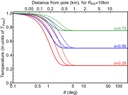
Figure 1: Synthetic profiles of the temperature (in units of $T_{\rm pole}$) on the surface of the NS as a function of the angle from the magnetic pole ($\theta=0\hbox{${}^{\circ}$}$). A range of profiles is shown here, with different values of $\epsilon$ and $n$ (see Equation 1): Red, Blue and Green curves correspond to $\epsilon=$ 0.25, 0.50, 0.75, respectively. The dotted, dashed and solid curves correspond to $n=$ 5000, 10000, 20000, respectively.

Single-pulse profiles with high pulse-fractions (PFs) such as that resulting from the observations of SGR 0418 cannot be readily explained by pairs of antipodal hot spots on the surface of the rotating NS. In fact, Beloborodov (2002) showed that two isotropically emitting, infinitesimal hot spots on the surface of a NS (of 1.4 solar masses and 10 km in radius) cannot produce PFs larger than about 12%. Poutanen & Beloborodov (2006) generalized the calculation to allow for anisotropy in the local emission, and obtained PFs of at most a few tens of percent. Similarly, DeDeo et al. (2001) studied the modulation level of the emitted flux as a function of the hot spot size, for two antipodal spots. They found that, for a NS of $1.4$ solar masses, radius 12.3 km, and a temperature contrast of $9$ between the spots and the rest of the surface, the PF can reach a maximum of $\sim 55$% if the local emission is strongly pencil-beamed, with an intensity $\propto\cos^{3}\delta$, where $\delta$ is the angle of the emitted photon with the normal to the surface. However, a more recent study was performed by Shabaltas & Lai (2012), using a family of parametrized temperature profiles with symmetry with respect to the equator. By employing a new method to efficiently compute the radiation intensity from different patches of a NS surface with arbitrary magnetic fields and effective temperatures, they were able to produce synthetic X-ray light curves for a variety of geometric configurations. In contrast to previous works, they were able to generate single-peaked profiles with PFs as high as $\sim 60\%$. They interpreted their findings as the result of diffuse hot spots of finite size (with varying temperatures), combined with the beaming due to anisotropic photon opacities in magnetic fields. We note that, consistently with previous work, their single pulsed profiles from symmetric temperature distributions displayed a plateau around the flux minimum. Using the same methodology of Shabaltas & Lai (2012), Storch et al. (2014) modelled the high X-ray PFs of the pulsar PSR B0943$+$10 by means of two asymmetric hot spots, a smaller one with stronger $B$ field, and a larger one with smaller $B$ field. Once again, the beaming effect of the atmosphere was found to be a crucial ingredient in producing a high modulation level.

We note that both the source Kes 79 analyzed by Shabaltas & Lai (2012), as well as the pulsar PSR B0943$+$10 modelled by Storch et al. (2014), had relatively well measured distances, and in addition, PSR B0943$+$10 had the viewing geometry constrained by radio observations. As a result, the area of the thermally emitting region could be well determined. On the other hand, the distance to SGR 0418 is rather uncertain. If located in the Perseus arm (which is in its direction), then the distance would be about 2$\,{\rm kpc}$ (van der Horst et al., 2010). However, there is no independent observational link to such an association. Because of this uncertainty, we choose to leave the distance to the source as a free parameter, which, as discussed in the following (see Section 4.1), will turn out to be correlated with the temperature profile on the NS surface, and especially with the size of the spot. In addition, given the characteristics of the source, and in particular its symmetric pulse profile (i.e. no evidence for a plateau around the minimum), as well as the very high PFs ($\sim 80\%$, and even consistent with $\sim 100\%$ above 1.2 keV), we focus our exploration on a family of temperature profiles asymmetric with respect to the equator, with one hemisphere hotter than the other. This choice is less restrictive in that it allows a wider range of sizes for the hotter component (and correspondingly a wider range of distances). However, we will also explore whether, similarly to the cases studied by Shabaltas & Lai (2012) and Storch et al. (2014), the viewing/emission geometry compatible with the data allows for the presence of a second antipodal hot region.

We begin by exploring the following family of temperature profiles

$$T\left(\theta\right)=\epsilon\;\mbox{$T_{\rm pole}$}+\left(1-\epsilon\right)\;\mbox{$T_{\rm pole}$}\;\cos^{n}\left(\frac{\theta}{2}\right),$$ (1)

where $\theta$ is the azimuthal angle, $\epsilon$ represents the fractional temperature difference between the two poles, and $n$ is an integer power which measures the gradient of the temperature decline between the two poles. Some representative profiles from this family are displayed in Figure 1, for different values of the parameters $\epsilon$ and $n$.

Similarly, the symmetric profiles (i.e., a pair of antipodal spots) are parametrized as

$$T\left(\theta\right)=\epsilon\;\mbox{$T_{\rm pole}$}+\left(1-\epsilon\right)\;\mbox{$T_{\rm pole}$}\;\cos^{n}\left({\theta}\right),$$ (2)

with $n$ constrained to be even.

We note that there is a certain degree of degeneracy between the gradient of the temperature profile, the local emission pattern of the radiation, the compactness $\mbox{$M_{\rm NS}$}/\mbox{$R_{\rm NS}$}$ of the NS, and the viewing geometry. For the local emission, we assume blackbody radiation with an analytical prescription for its beaming. We realize that this is an approximation in the case that the star has an atmosphere, which processes the surface radiation creating a distorted blackbody and modifying the emission pattern. The only correct way to approach this problem would be to generate a magnetized atmosphere model for each patch of the star (different $B$ and $T$). To the best of our knowledge, this has been done only with an approximate method to produce realistic pulsed profiles coupled with analytical temperature/magnetic profiles (Shabaltas & Lai, 2012; Storch et al., 2014). However, it is impractical to implement this method while formally fitting data since it would require the computation of a much larger number of atmospheric profiles than done in those papers (we will be minimizing over a wide grid of parameters for both the temperature profile and the viewing geometry). On the other hand, using a single model atmosphere (i.e., a single strength for $B$ and one direction, perpendicular to the normal) on the entire surface – which is reasonably easy to do in a fit – would be generally incorrect, and especially so if the object has a significant non-radial component of the external magnetic field. Therefore, given that the detailed magnetic topology of SGR 0418 is not apriori known, and the fact that, even with a perfect spectral computation there would still remain a degree of degeneracy in the pulsed profiles with the compactness ratio of the star (which we assume fixed at some typical value), and the viewing geometry, which we constrain by fitting the pulse profile, we adopt the simplest approach of assuming local blackbody emission with a parametrized form for the beaming which captures the ’limb-darkening’ effect of magnetized, light-element atmospheres (see also Bogdanov 2014 for a similar approach). However, in order to quantify the dependence of the results we obtain on the presence of beaming, we will also repeat part of the analysis for isotropic emission.

2.2 General-relativistic, phase-dependent spectra

The general relativistic, phase-dependent spectra are calculated using the formalism developed by (Page 1995, see also Pechenick et al. 1983; Pavlov & Zavlin 2000). The intense gravitational field of the star bends the photon trajectories: a photon emitted at an angle $\delta$ with the normal to the NS surface will reach a distant observer if generated at an angle $\theta_{v}$ with respect to the viewing axis, where

$$\theta_{v}(\delta)=\int_{0}^{\frac{R_{s}}{2R}}x\left[\left(1-\frac{R_{s}}{R}\right)\left(\frac{R_{s}}{2R}\right)^{2}-(1-2u)u^{2}x^{2}\right]^{-\frac{1}{2}}\mbox{d}u\,.$$ (3)

In the above equation, $x\equiv\sin\delta$, $R_{s}\equiv 2GM/c^{2}$ is the Schwarzschild radius of the star, and $R$ and $M$ are, respectively, its radius and mass. Here we adopt a canonical mass $M=1.4\mbox{$\,M_{\odot}$}$ and radius $R_{\rm NS}$=10$\,{\rm km}$. These values yield a gravitational redshift $(1-R_{s}/R)^{1/2}=0.766$. Correspondingly, a distant observer would measure a radius of $\mbox{$R_{\infty}$}=R\times({1-{{R_{s}}/{R}}})^{-1/2}=13.1\hbox{$\,{\rm km}$}$, and a surface temperature of $T_{\infty}=T\times(1-R_{s}/R)^{1/2}$. In the following, we will quote fit results for the pole temperature in terms of the redshifted values, $T_{{\rm pole},\infty}$.

Let $\Omega(t)$ be the modulus of the NS angular velocity, and let us define the phase angle $\gamma(t)=\int\Omega(t)dt$ as the azimuthal angle subtended by a reference vector ${\bf\hat{n}}$ around the axis of rotation. As the reference vector, we choose the polar axis, in the coordinate system in which $T(\theta=0)\equiv\mbox{$T_{\rm pole}$}$. For a dipolar component of the magnetic field, this would correspond to the magnetic axis; for the toroidal component of the field, it represents the symmetry axis.

As the star rotates, the angle between the vector ${\bf\hat{n}}$ and the line of sight is given by

$$\alpha(t)=\arccos\left[\cos\psi\cos\xi+\sin\psi\sin\xi\cos\gamma(t)\right]\,,$$ (4)

where we indicated by $\psi$ and $\xi$ the angles that the rotation axis respectively makes with the line of sight and ${\bf\hat{n}}$ (see Figure 1 in Perna & Gotthelf 2008 for a graphical representation of the viewing geometry). Note that there is a degeneracy between the two angles $\psi$ and $\xi$, i.e., they can be exchanged without altering the pulse-profile or the spectra.

The phase-dependent spectrum measured by the observer as the star rotates is obtained by integrating the local emission over the entire observable surface. Accounting for the effect of gravitational redshift of the emitted radiation, this integral takes the form

$$F(E_{\infty},\alpha)=\frac{E_{\infty}^{2}}{c^{2}h^{3}}\frac{R_{\infty}^{2}}{D^{2}}\;\int_{0}^{1}2x\int_{0}^{2\pi}I\{T[\theta_{v}(x),\phi_{v}],E\}\,\mbox{d}\phi_{v}\mbox{d}x\,,$$ (5)

where $D$ is the distance, $E_{\infty}=E({1-{{R_{s}}/{R}}})^{1/2}$ is the energy measured by a distant observer, the spectral function $I[T(\theta_{v},\phi_{v}),E]$ describes the dimensionless distribution of the locally emitted photons (the blackbody function here), and $(\theta_{v},\phi_{v})$ are the coordinates on the surface relative to the line of sight.

As discussed above, to emulate the effect of a magnetized, light-element atmosphere, we assume the local photon intensity to emerge in a pencil-beaming pattern with respect to the normal to the surface, which we model as $f(\delta)\propto\cos^{p}\delta$, with a beaming intensity $p=1$ as a closer match to that of realistic, magnetized atmosphere models (van Adelsberg & Lai, 2006).

From Equation (5), other useful quantities for comparison to observations can then be readily computed. In particular, the phase-averaged spectrum is given by

$$F_{\rm ave}(E_{\infty})=\frac{1}{2\pi}\;\int_{0}^{2\pi}\;F[E_{\infty},\alpha(\gamma)]\;d\gamma\;,$$ (6)

while the pulse profile in a given (observed) energy band, $\{E_{1,\infty},E_{2,\infty}\}$, is

$$F(\gamma)=\int_{E_{1,\infty}}^{E_{2,\infty}}\;F[E_{\infty},\alpha(\gamma)]\;dE_{\infty}.$$ (7)

The PF is defined as

$${\rm PF}=\frac{F_{\rm max}(\gamma)-F_{\rm min}(\gamma)}{F_{\rm max}(\gamma)+F_{\rm min}(\gamma)}\;,$$ (8)

where the phases corresponding to the maximum and minimum of the flux will generally vary depending on the temperature distribution on the NS surface.

Table 1: XMM-Newton Observations of SGR 0418$+$5729

ObsID	Start	Usable time
	Time (TT)	(ksec)
0693100101	2012-08-25 14:18:08	58.7
0723810101	2013-08-15 18:06:25	32.5
0723810201	2013-08-17 20:57:17	36.0

3 Data reduction and description of analyses

3.1 XMM-Newton observations

We use in this work two recent observations of SGR 0418 with XMM-Newton, acquired in August 2012 and August 2013 (see Table LABEL:tab:ObsID), when the source appears to have approached quiescence with a stable flux. All observations were acquired with the EPIC-pn camera (Strüder et al., 2001) in Large Window mode, i.e., with a time frame of 48$\,{\rm ms}$, and with the EPIC-MOS cameras (Turner et al., 2001) in Small Window mode, with a time resolution of 300$\,{\rm ms}$. For the timing analysis, data from both pn and MOS cameras are used, while only the pn spectrum is used for the spectral analysis.

Standard reduction procedures are applied, using epchain in the XMMSAS v13.5 package, together with the latest calibration files. Photon events times of arrival are corrected to the Solar System barycenter, using barycen, before the phases of all events are calculated using the best-fit X-ray timing solution reported in Rea et al. (2013): $P=9.07838822\mbox{$\,{\rm sec}$}$, $\dot{P}=4\mbox{$\times 10^{-15}$}\mbox{$\,{\rm sec}$}\mbox{$\,{\rm s^{-1}}$}$ on MJD 54993.0. The data were checked for background flares, which were removed to limit contamination. The resulting usable exposure times for each observation are listed in Table LABEL:tab:ObsID. Finally, events are filtered in the 0.3–10.0$\,{\rm keV}$ range with the PATTERN $\leq$4 and FLAG = 0 restrictions. The observed flux of both observations is consistent with being constant, confirming that SGR 0418’s luminosity and surface temperatures have not significantly changed between observations.

Figure 2: Phase averaged spectral fit with the model described in Section 2 (see Equation 5), with $n=12783$, $\epsilon=0.08$ and $(\psi,\,\xi)=(13\hbox{${}^{\circ}$},84\hbox{${}^{\circ}$})$, the most likely values from Section 4.2. The spectral shape is mostly driven by the pole temperature $T_{\rm pole}$ and the absorption column density $N_{\rm H}$, while the flux depends on $n$ and $\epsilon$ with weaker dependence on $\psi$ and $\xi$. The fit is statistically acceptable with $\chi^{2}_{\nu}$/dof (prob.) = 1.28/34 (0.13).

3.2 Spectral analysis

Phase-averaged spectra are extracted from the two observations in the 0.3–10$\,{\rm keV}$ range using 20^′′ circular regions. Background spectra are extracted from 90^′′ circular regions devoid of X-ray sources. The response matrices were generated using the tools rmfgen and arfgen. The extracted pn spectra are then combined into a single spectra using epicspeccombine, after verification that the flux was consistent with being constant. Finally, events are binned for the purpose of the phase-averaged spectral analysis with a minimum of 20 counts per bins. For the spectral analysis performed in XSPEC v.12.8 (Arnaud, 1996), 3% systematics are added in each spectral bin to account for uncertainties in the absolute flux calibration of the instrument (Guainizzi, 2014). The spectral model used, described in Section 2, is modulated by X-ray absorption using the wabs model (Morrison & McCammon, 1983). The overall normalization factor of the fit, convoluted with the uncertain distance to the source, is left free to vary. All errors from the spectral analysis are at the 90% confidence level. The spectrum and best-fit model are shown in Figure 2, and the results are presented in Section 4.

3.3 Pulse Profile Analysis

The phases resulting from the folding at the timing solution given above are used to generate the pulse profile. Furthermore, because of the low count rates in the observations, we limit the analysis to 10 phase bins. The errors in the number of counts in each bin are Poisson errors. The average background number of counts is subtracted in each phase bin. For the background subtraction, the background regions used have the same size as the SGR 0418 source regions, and are devoid of any other detected X-ray source.

The PF is calculated according to Equation (8), where $F_{\rm max}(\gamma)$ and $F_{\rm min}(\gamma)$ are the maximum and minimum X-ray fluxes measured in the phase bins. The PF for the cumulative 0.3–10$\,{\rm keV}$ band is $PF=0.78\pm 0.09$. While first using the single 0.3–10$\,{\rm keV}$ band for the computation of the pulsed profile and modelling, we then also considered splitting the full energy range into smaller bands, since this carries a higher constraining power for the underlying model. However, we found that splitting in more than two bands would result in a too low count rate per band. Hence we limited the split to only two bands, 0.3–1.2$\,{\rm keV}$ and 1.2–10.0$\,{\rm keV}$, which were chosen to have approximately similar count rates. We found the PF in the lower energy band to be $PF_{0.3-1.2\,{\rm keV}}=0.62\pm 0.10$, while the higher band $PF_{1.2-10.0\,{\rm keV}}$ was consistent with $1.0$. As expected, the PF in the high-energy band is higher than in the low-energy band.

4 Constraining the surface temperature through spectral and pulse profile modelling

4.1 Iterative fitting of spectra and pulse profiles

Constraining the temperature profile requires a coupled spectral and timing analysis. The pulsed profiles are most sensitive to the run of temperature with angle on the NS surface, while the phase-averaged spectra are most sensitive to the overall flux normalization (reflected in $T_{\rm pole}$ and on the size of the spot, for a fixed NS radius), and to the amount of absorption, quantified by the column density of hydrogen $N_{\rm H}$, noted $N_{H,22}$ hereafter when expressed in units of $10^{22}$$\rm\,{\rm atoms}\mbox{$\,{\rm cm^{-2}}$}$. Once $T_{\rm pole}$ and $N_{\rm H}$ are measured from the spectra, fitting the synthetic pulse profiles (computed via Equation 7) to the observed pulse profiles allows to constrain the system geometry and the temperature profile. Here, we first perform the spectral and timing analysis iteratively rather than simultaneously. We will show that this is a rather good approximation indeed (see also Bernardini et al. 2011). However, Section 4.2 will present and validate a simultaneous analysis using a Markov-Chain Monte-Carlo approach.

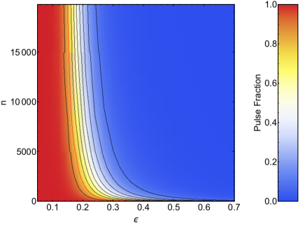
Figure 3: Pulsed fractions (PFs) obtained as a function of the parameters $n$ and $\epsilon$, with the system geometry $(\psi,\,\xi)=(90\hbox{${}^{\circ}$},90\hbox{${}^{\circ}$})$, which maximizes the PF. Contour lines indicate PFs ranging from 0.1 to 0.9, with 0.1 increments; the red line indicates the 0.8 PF contour. Note that while the low range of $n$ values can produce PF such as those observed for SGR 0418, it fails to accomodate reasonable distances of this source (see discussion in Section 4.1).

Using the spectral model described in Section 2, together with the family of temperature profiles defined by Eq. (1), we first obtain an estimate of $T_{\rm pole}$ and $N_{\rm H}$ from a small selection of surface temperature distributions, for a viewing geometry $\left(\psi,\xi\right)=\left(90\hbox{${}^{\circ}$},90\hbox{${}^{\circ}$}\right)$. In the first step of the iteration the viewing geometry is not constrained yet, and the choice of an orthogonal rotator is made as a starting point given the high PF of the source. We find that for a fixed distance (e.g. $2\mbox{$\,{\rm kpc}$}$), the spectra strictly constrain the values of $\epsilon$ and $n$ such that the model produces the flux observed for this source. This is because these parameters relate to the fraction of the NS surface which dominates the emission (see Figure 1), and hence to the fit normalization. In other words, the shape of the observed spectra constrains the average emission temperature and absorption, while the flux normalization restricts the size of the spot and the temperature constrast at the surface. We note, however, that the distance is estimated solely based on the association of the magnetar with the Perseus arm of the Galaxy. This assumption stems from the position of SGR 0418 in the direction of the Perseus arm. Should this association be fortuitous, the distance to SGR 0418 could be mis-estimated to lower or higher values.

Such uncertainties in the distance translate into less constrained parameters $\epsilon$ and $n$. As an example, a spectral fit with $\epsilon=0.1$, $n=10,000$ (i.e., a spot size of $0.275\hbox{$\,{\rm km}$}$, full-width at half-maximum, FHWM, on a 10$\,{\rm km}$ NS) yields a distance of $2.13\mbox{$\,{\rm kpc}$}$, while a fit with $\epsilon=0.15$, $n=5,000$ (spot size of $0.425\hbox{$\,{\rm km}$}$ FWHM) yields $4.9\mbox{$\,{\rm kpc}$}$. However, the parameters $T_{\rm pole}$ and $N_{\rm H}$ appear relatively stable against change in $\epsilon$ and $n$, or in the viewing geometry. We find $\mbox{$T_{{\rm pole},\infty}$}\sim 0.32\mbox{$\,{\rm keV}$}$ and $\mbox{$N_{H,22}$}\sim 0.25$ for a wide range of $\epsilon$ and $n$ that lead to reasonable values of the distance ($d\sim 0.5-4\mbox{$\,{\rm kpc}$}$), i.e., $\epsilon\mbox{$\,{}^{<}_{\sim}\,$}0.10-0.15$ and $n\sim 5000-20000$. Therefore we already have a good starting point in this iterative process to constrain the parameters of the system. Higher values of $\epsilon$ lead to statistically unacceptable fits.

We note the existence of a secondary $\chi^{2}$ minimum, leading to acceptable fit statistics, in which $\mbox{$N_{H,22}$}\sim 1.2$ corresponds to $\epsilon\sim 0.4$, for the same pole temperature. This could be explained by the fact that the larger averaged flux created by the less pronounced contrast (larger $\epsilon$) needs to be heavily absorbed to fit the data. However, we reject such a large value of the absorption, on account of the fitted values of $N_{\rm H}$ from the high signal-to-noise observations obtained during the outbursts (Rea et al., 2013).

With the estimated values of pole temperature and absorption, we can then explore the $\epsilon$–$n$ parameter space for pairs capable of accomodating a PF of $\sim 0.80$. Figure 3 shows the PF as a function of $\epsilon$ and $n$ for $\left(\psi,\xi\right)=\left(90\hbox{${}^{\circ}$},90\hbox{${}^{\circ}$}\right)$. With such angles, a $PF\sim 0.80$ can be reproduced for a wide range of $n$, while $\epsilon$ remains essentially constant at $\sim 0.15$.

We note that the high measured PF of the source is partly due to the effect of X-ray absorption. More specifically, absorption can artificially increase the intrisic (unabsorbed) PF since the low-temperature portion of the NS surface (emitting lower energy, less pulsed X-ray photons) is more affected by absorption than the hotter parts. The artifical increase in PF due to absorption depends both on the geometry $\left(\psi,\xi\right)$ and the temperature gradient on the star. The emission model of this analysis can be used to estimate the intrinsic PF of SGR 0418, i.e., unaffected by absorption. Specifically, for $n=10000$ and $\epsilon=0.15$, the intrinsic PF is 0.36, while it is 0.88 for $\mbox{$N_{H,22}$}=0.25$, hence quite sensitive to $N_{\rm H}$.

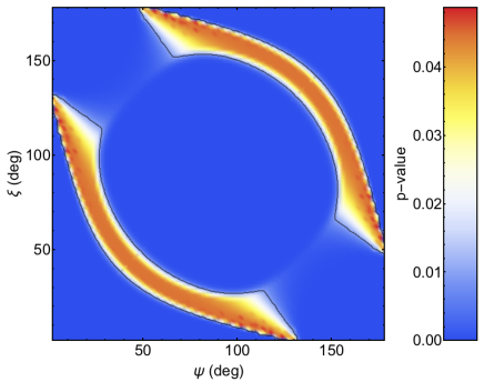
Figure 4: Projected 2D map of maximum p-values when the two angle $\psi$ and $\xi$ vary, in the case of beamed local emission (pencil beam $\propto\cos\delta$). The solid line represents the probability $p=0.01$. The best-fit over the whole 4D-space corresponds to a p-value $p=0.05$.

Next, choosing $\psi=90\hbox{${}^{\circ}$}$ and $\xi=90\hbox{${}^{\circ}$}$ with the temperature distribution profile defined by $\epsilon=0.15$ and $n=10000$, we perform a detailed spectral analysis in order to further refine the value of the pole temperature $T_{\rm pole}$ and the X-ray absorption $N_{\rm H}$. An acceptable fit to the data is obtained with $\mbox{$T_{{\rm pole},\infty}$}=0.33\mbox{${}^{+0.05}_{-0.05}$}\mbox{$\,{\rm keV}$}$ and $\mbox{$N_{H,22}$}=0.36\mbox{${}^{+0.09}_{-0.07}$}$ (see Figure 2). However, a better fit is obtained with $\epsilon=0.10$ and $n=10000$ leading to $\mbox{$T_{{\rm pole},\infty}$}=0.38\mbox{${}^{+0.05}_{-0.05}$}\mbox{$\,{\rm keV}$}$ and $\mbox{$N_{H,22}$}=0.22\mbox{${}^{+0.09}_{-0.07}$}$ for $\chi^{2}_{\nu}$/dof (prob.) = 1.28/34 (0.13). The flux of SGR 0418 is $\mbox{$F_{\rm X}$}=2.0\mbox{${}^{+0.4}_{-0.4}$}\mbox{$\times 10^{-14}$}\mbox{$\,{\rm erg\,\mbox{$\,{\rm cm^{-2}}$}\,\mbox{$\,{\rm s^{-1}}$}}$}$ in the 0.3–3.0$\,{\rm keV}$ range. Although these values of $n$ and $\epsilon$ slightly overpredict the PF (see Figure 3), the best-fit $T_{\rm pole}$ and $N_{\rm H}$ are consistent with those estimated for different values of $\epsilon$ and $n$ in the first step of this iterative process.

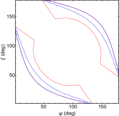
Figure 5: Same as in Figure 4, but for the two bands: 0.3–1.2$\,{\rm keV}$ (red) and 1.2–10.0$\,{\rm keV}$ (blue). Only the $p=0.01$ contours are plotted to allow comparison between the two bands.

With the values of $\mbox{$T_{{\rm pole},\infty}$}=0.38\mbox{$\,{\rm keV}$}$ and $\mbox{$N_{H,22}$}=0.22$ obtained from the spectral analysis, we next proceed to constrain the system geometry and the temperature distribution that best reproduces the pulsed emission from the surface of SGR 0418. For the analysis that we describe in the following, we first consider the pulsed profile in the full energy band 0.3–10$\,{\rm keV}$. Using the model described in Section 2, a grid of pulse profiles is generated for multiple system geometries (varying the angles $\psi$ and $\xi$ between 2^∘and 180^∘, in steps of $2\hbox{${}^{\circ}$}$), and multiple temperature distribution profiles (by varying $n$ between 5000 and 20000 in steps of 500, and $\epsilon$ between 0.05 and 0.15 in steps of 0.01). Each of the synthetic pulse profiles generated for each set of 4 parameters ($\psi$, $\xi$, $n$, $\epsilon$) is then fitted to the observed XMM-Newton pulse profile. From the $\chi^{2}$ values obtained from these fits, projected 2-dimensional maps of maximum p-values are obtained.

Figure 4 shows the maximum p-value maps for the pair of angles $\psi$-$\xi$. The fit to the pulsed profile allowed us to mainly constrain the viewing/inclination geometry. The parameters $n$ and $\epsilon$ were not constrained by the pulse profile fitting any further than what was imposed by the spectral analysis (via the distance requirement). In other words, $n$ and $\epsilon$ were essentially unconstrained by the pulse profile fitting in the range 5000–20000 and 0.05–0.15, respectively.

The best-fit resulting from the grid search in the parameter space is obtained for the following parameters: $\epsilon=0.10$, $n=7500$ for $\left(\psi,\xi\right)=\left(\xi,\psi\right)=\left(124\hbox{${}^{\circ}$},4\hbox{${}^{\circ}$}\right)$, with $\chi^{2}_{\nu}$/dof (prob.) = 1.9/8 (0.05). However, as can be observed in Figure 4, a wide range of angles is permitted by the pulse profile fitting ($p>0.01$), with very different sets of parameters $n$ and $\epsilon$. Figure 4 also shows that the angles $\psi$ and $\xi$ are constrained to two narrow bands. Note the observed symmetry emerges from the symmetry against exchanges between $\psi$ and $\xi$ (see Equation 1). The most conservative constraints on the angles can be summarized by the intervals: $73\hbox{${}^{\circ}$}\mathrel{\hbox{\hbox to0.0pt{\hbox{\lower 4.0pt\hbox{$\sim$}}\hss}\hbox{$<$}}}\psi+\xi\mathrel{\hbox{\hbox to0.0pt{\hbox{\lower 4.0pt\hbox{$\sim$}}\hss}\hbox{$<$}}}140\hbox{${}^{\circ}$}$ and $220\hbox{${}^{\circ}$}\mathrel{\hbox{\hbox to0.0pt{\hbox{\lower 4.0pt\hbox{$\sim$}}\hss}\hbox{$<$}}}\psi+\xi\mathrel{\hbox{\hbox to0.0pt{\hbox{\lower 4.0pt\hbox{$\sim$}}\hss}\hbox{$<$}}}287\hbox{${}^{\circ}$}$.

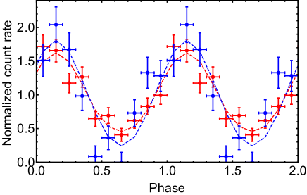
Figure 6: Background subtracted pulse profile of SGR 0418 in the energy range 0.3–1.2$\,{\rm keV}$ (red) and 1.2–10.0$\,{\rm keV}$ (blue). The dashed line corresponds to the best synthetic pulse profiles obtained from the grid search described in Section 4.1 for each of the two energy bands.

A consistency check was then performed by using the values of the best-fit angles $\left(124\hbox{${}^{\circ}$},4\hbox{${}^{\circ}$}\right)$ and temperature distribution parameters ($n=7500$ and $\epsilon=0.10$) in a phase-averaged spectral fit. These parameters lead to a best-fit temperature $\mbox{$T_{{\rm pole},\infty}$}=0.34\mbox{${}^{+0.03}_{-0.03}$}\mbox{$\,{\rm keV}$}$ and a hydrogen column density $\mbox{$N_{H,22}$}=0.30\mbox{${}^{+0.06}_{-0.04}$}$, for a corresponding distance of $0.5\mbox{$\,{\rm kpc}$}$. The pole temperature and the hydrogen column density remain consistent with the best-fit $T_{\rm pole}$ obtained when fixing $\left(\psi,\xi\right)=\left(90\hbox{${}^{\circ}$},90\hbox{${}^{\circ}$}\right)$, as done at the beginning of this iterative analysis. In addition, for the best-fit temperature distribution found above ($n=7500$ and $\epsilon=0.10$), the viewing geometry appears to have an effect on the distance (i.e. flux normalization). For $\left(\psi,\xi\right)=\left(124\hbox{${}^{\circ}$},4\hbox{${}^{\circ}$}\right)$, $d=0.5\mbox{${}^{+0.1}_{-0.1}$}\mbox{$\,{\rm kpc}$}$ and for $\left(\psi,\xi\right)=\left(90\hbox{${}^{\circ}$},20\hbox{${}^{\circ}$}\right)$, $d=2.7\mbox{${}^{+1.0}_{-0.9}$}\mbox{$\,{\rm kpc}$}$ (these uncertainties are essentially flux uncertainties). While this was not suspected initially, this dependence of the distance on the viewing geometry is explained by the fact that a highly contrasted spot, more or less-often visible during a complete phase depending on the viewing angles, will correspondingly generate a larger or smaller flux in the phase averaged spectra.

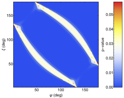
Figure 7: Same as in Figure 4, but in the case of an isotropic local emission.

The grid search described above was then repeated with the pulse profiles computed in the two energy bands 0.3–1.2$\,{\rm keV}$ and 1.2–10.0$\,{\rm keV}$. The resulting best fits pulse profiles are shown in Figure 6, and the 2D projections of maximum p-values are displayed in Figure 5. The analysis of the pulse profiles in the two bands shows that the higher energy bands constrain the angles a little more than the low energy band and this is simply due to the larger pulse fraction (consistent with 1.0) observed in the 1.2–10.0$\,{\rm keV}$ band compared to the 0.3–1.2$\,{\rm keV}$ band. But overall, the parameter space is mostly insensitive to the energy band chosen, given the low signal-to-noise available in these obervations.

Last, with the purpose of quantifying the effect that the uncertain atmospheric beaming has on our results, we repeat the analysis assuming local isotropic emission. This results in a narrower allowed parameter space for the angles $\psi$ or $\xi$. For example, we find that the angles $\psi$ or $\xi$ must lie in the range $104\hbox{${}^{\circ}$}\mathrel{\hbox{\hbox to0.0pt{\hbox{\lower 4.0pt\hbox{$\sim$}}\hss}\hbox{$<$}}}\psi+\xi\mathrel{\hbox{\hbox to0.0pt{\hbox{\lower 4.0pt\hbox{$\sim$}}\hss}\hbox{$<$}}}145\hbox{${}^{\circ}$}$ and $215\hbox{${}^{\circ}$}\mathrel{\hbox{\hbox to0.0pt{\hbox{\lower 4.0pt\hbox{$\sim$}}\hss}\hbox{$<$}}}\psi+\xi\mathrel{\hbox{\hbox to0.0pt{\hbox{\lower 4.0pt\hbox{$\sim$}}\hss}\hbox{$<$}}}256\hbox{${}^{\circ}$}$. Moreover, the contours are less curved in $\psi$–$\xi$ space (Figure 7). These results can be understood since the effect of beaming is that of creating a larger modulation for the same parameters. Hence, to reproduce the same level of observed modulation with a local isotropic emission beaming, smaller viewing angles are not allowed, restricting the angle geometry to larger values.

The best-fit pulse profiles in the locally isotropic [$\chi^{2}_{\nu}$/dof (prob.) = 1.9/8 (0.06)] and pencil-beamed surface emission are compared in Figure 8. As it can be seen, the profiles are almost indistinguishable. This result stems from what just discussed above: when the local emission is beamed, the fit parameters adjust so that smaller viewing angles/temperature contrast are needed to achieve the same observed level of modulation. Therefore, a comparison between Figure 4 and 7 yields a quantitative estimate of the amount by which the uncertain angular distribution of the local emission affects the inferred system parameters.

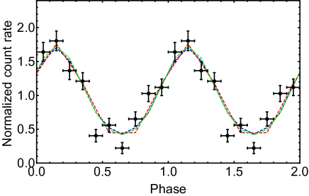
Figure 8: Background subtracted pulse profile of SGR 0418, together with the best fit synthetic pulse profiles obtained from the grid search described in Sections 4.1 and 4.3 (dashed blue: single spot with pencil-beamed surface emission, dashed red: single spot with isotropic surface emission, dashed green: two spots with pencil-beamed surface emission). They are computed in the 0.3–10$\,{\rm keV}$ band.

4.2 Simulateneous fitting of spectra and pulse profiles using a Markov-Chain Monte-Carlo approach

As explained in Section 4.1, the source spectrum is more sensitive to some parameters of the model (e.g.: $T_{\rm pole}$ or the spot size charaterized by $n$ in Equation 1) while the pulse profile is more sensitive to variations in the temperature contrast at the surface or in the system geometry ($\psi$ or $\xi$). Nonetheless, all parameters play a role in modelling the surface emission and its phase- and energy- dependence, and Section 4.1 showed that it was somewhat difficult to predict what variations of a given parameter can have on the modelled pulse profile or spectrum. Iterating between pulse profile and spectral fits proved to be impractical due to the number of parameters. Furthermore, a simultaneous analysis allows us to have a global understanding on the roles of parameters in the model, and to better understand the existing degeneracies between parameters. For these reasons, a Markov-Chain Monte Carlo (MCMC) approach was then employed to sample the parameter space while simultaneously fitting the spectra and pulse profiles. In addition, the method allows to include known priors on some of the parameters.

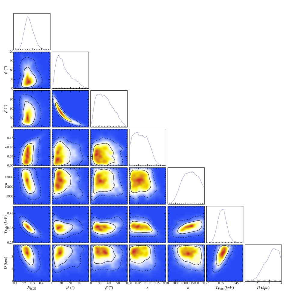
Figure 9: 2-dimensional posterior distributions for each pair of parameters and 1-dimensional posterior distributions for each parameter resulting from the simultaneous fits of the pulse profiles and spectra via the MCMC approach described in Section 4.2. The color scales of the 2-dimensional posterior distributions represent the density of points (i.e., blue means zero-density), compared to other figures of this article where the color scales represent the p-values. The solid and dashed contours are enclosing 68% and 95% of the accepted points. This figure was created with the Mathematica package LevelSchemes (Caprio, 2005).

The implementation of the MCMC algorithm used in this work, the “Stretch-Move” algorithm (also called “Affine Invariant Ensemble Sample”, Goodman & Weare, 2010), was previously employed, described and tested extensively in other works (e.g., Wang et al., 2013; Guillot et al., 2013; Guillot & Rutledge, 2014). It made use of the PyXSPEC package, the python version of XSPEC (Arnaud, 1996), for the comparison of the synthetic spectra to the phase-average spectra. In this algorithm, multiple chains (called “walkers”) are sampling the parameter space and each set of proposed parameters is accepted or rejected based on the likelihood of the model with the proposed sets of parameters. The next proposed step of each chain is then chosen from an affine invariant distribution along a line between the current point of the chain and the current point of a randomly chosen chain.

In this approach, we used a set of seven parameters sampled by the MCMC:

• the two angles of the system geometry $\psi$ and $\xi$ (constrained to $\psi+\xi<180\hbox{${}^{\circ}$}$, as justified by the symmetry, in Eq. (4); this is to reduce the size of the parameter space explored, and the full range can be recovered by symmetry).

• the surface temperature contrast $\epsilon$ (Eq. 1),

• the parameter $n$ characterizing the spot size (Eq. 1),

• the column density of hydrogen $N_{\rm H}$,

• the pole temperature $T_{\rm pole}$,

• the distance $d$, for which we choose a flat prior between 0.5 and 4$\,{\rm kpc}$ (see discussion in Section 4.1).

The neutron star radius, which controls the star’s compactness and therefore the amount of light-bending, could also be sampled in this approach to potentially obtain some constraints on its value. However, it was held fixed here due to the relatively low signal-to-noise ratio of the data. Higher signal-to-noise data could potentially place constraints on the radius, although there exists degeneracies with the angle geometry that would not be fully broken (see e.g., Perna & Gotthelf 2008; Bernardini et al. 2011).

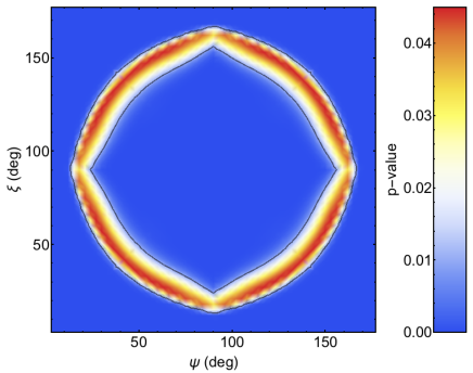
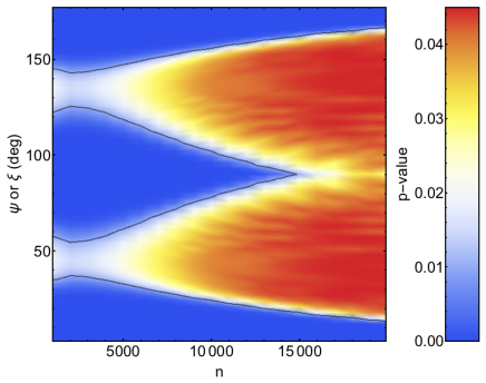
Figure 10: (left) Similar to Figure 4 but for a symmetry temperature distribution representing two antipodal spots. The solid line represents the probability $p=0.01$. (right) Projected map of maximum p-values in a $n$–$\psi$ or $n$–$\xi$ space.

In this MCMC simulation, 50 walkers were run simultaneously for a total of 15000 steps each. After removing 5000 steps of burn-in, an average acceptance rate of 15% was obtained. We also checked for convergence by visually inspecting the trace of each parameter. The results of this simultaneous analysis of the pulse profiles and spectra of SGR 0418 with our model are shown in Figure 9, as the 1-dimensional and 2-dimensional posterior distributions of all parameters.

This simultaneous analysis confirms what has been observed in the iterative method of Section 4.1. In particular, the constraint on the geometry of the system (see the $\psi-\xi$ plot of Figure 9) is well reproduced, albeit with a slightly different shape that results from the coupled constraints from the spectra (as noted in Section 4.1, the distance and the angle geometry are related). The constraints on the two angles are: $65\hbox{${}^{\circ}$}\mathrel{\hbox{\hbox to0.0pt{\hbox{\lower 4.0pt\hbox{$\sim$}}\hss}\hbox{$<$}}}\psi+\xi\mathrel{\hbox{\hbox to0.0pt{\hbox{\lower 4.0pt\hbox{$\sim$}}\hss}\hbox{$<$}}}125\hbox{${}^{\circ}$}$ or $235\hbox{${}^{\circ}$}\mathrel{\hbox{\hbox to0.0pt{\hbox{\lower 4.0pt\hbox{$\sim$}}\hss}\hbox{$<$}}}\psi+\xi\mathrel{\hbox{\hbox to0.0pt{\hbox{\lower 4.0pt\hbox{$\sim$}}\hss}\hbox{$<$}}}295\hbox{${}^{\circ}$}$.

Furthermore, because a conservative prior on the distance was included, the size of the spot (parametrized via $n$) is not particularly well constrained. We find that the spot size is in the range 1.2^∘–3.8^∘, equivalent to $0.2-0.7\hbox{$\,{\rm km}$}$ for the 10-km NS considered here. The spot size distribution peaks at $0.35\hbox{$\,{\rm km}$}$. We note that allowing for larger distances would therefore include larger spot sizes (i.e, smaller values of $n$) in the posterior distributions. Since this is driven by the spectra normalization, it would not affect significantly the posterior distributions of $T_{\rm pole}$ or $N_{\rm H}$. However, a consequence would be a broadening of the “banana”-shape contours of the 2D-distribution of $\psi$–$\xi$, since a larger spot would reproduce the pulse profiles for larger values of the angles $\psi$ and $\xi$. Note also that because of the symmetry arising from the system geometry, the angles in the MCMC run were constrained to $\psi+\xi<180\hbox{${}^{\circ}$}$, and therefore, the $\psi-\xi$ plot only shows one of the “banana” shape contours.

The temperature contrast $\epsilon$ is constrained to similar values as those obtained in the iterative analysis, i.e. $\epsilon\mathrel{\hbox{\hbox to0.0pt{\hbox{\lower 4.0pt\hbox{$\sim$}}\hss}\hbox{$<$}}}0.15$. However, it is important to note that while allowed here, $\epsilon\rightarrow 0.0$ represents an unphysical description of the temperature distribution at the surface of the NS since the cold part cannot have a zero temperature. Furthermore, given the posterior 2D distributions of Figure 9, one can readily see that excluding the lower range of $\epsilon$, say 0.00–0.05, would not significantly affect the other parameters due to the mild correlation between $\epsilon$ in this range and the other parameters.

The posterior distribution of the pole temperature is $\mbox{$T_{{\rm pole},\infty}$}=0.36\pm{0.05}\mbox{$\,{\rm keV}$}$ (90% c.l.) while the hydrogen column density is $\mbox{$N_{H,22}$}=0.25\mbox{${}^{+0.12}_{-0.08}$}$ (90% c.l.). Note that we initially observed the bimodal distribution of $N_{\rm H}$ and therefore $\epsilon$ (leading to the secondary $\chi^{2}$ minimum in the spectral fit described in Section 4.1). We then applied a prior on $N_{\rm H}$ to exclude values $\mbox{$N_{H,22}$}>0.8$ (see Section 4.1). The distance is slightly more constrained than the initially prior range allowed. We find a distribution between 1.5$\,{\rm kpc}$ and 4$\,{\rm kpc}$, skewed toward larger values. Nonetheless, the 2$\,{\rm kpc}$ distance suggested if SGR 0418 indeed resides in the Perseus arm cannot firmly excluded.

Finally, the best-fit is obtained for the following set of parameters: $\mbox{$N_{H,22}$}=0.24$, $\psi=96.8\hbox{${}^{\circ}$}$, $\xi=7.9\hbox{${}^{\circ}$}$, $\epsilon=0.08$, $n=16961$, $\mbox{$T_{{\rm pole},\infty}$}=0.38\mbox{$\,{\rm keV}$}$ and $d=2.27\mbox{$\,{\rm kpc}$}$, corresponding to a fit statistic $\chi^{2}_{\nu}$/dof (prob.) = 58.5/38 (0.02). However, it is crucial to keep in mind that the full posterior distributions are the true representation of the acceptable parameter space given the model chosen and the data.

Overall, this technique is superior to the iterative process of Section 4.1 since it includes all the effects of parameter variations on both the pulse profiles and spectra, which proved too difficult to perform iteratively. Nonetheless, the iterative analysis performed initially provided a validation of the simultaneous analysis via MCMC.

4.3 Can two antipodal spots be responsible for the observed pulse profile of SGR 0418?

We present here an analysis similar to that of Section 4.1 but with a symmetric temperature distribution at the surface of the magnetar (Equation 2), i.e., with two antipodal spots. As can be seen in Figure 10 (left panel), the two-spots temperature distribution is able to accomodate the observed pulse profile for a narrow range of angles. One can note the additional symmetry (compared to the single spot case) since the two spots are identical. The two angles $\psi$ and $\xi$ are constrained to be $\mathrel{\hbox{\hbox to0.0pt{\hbox{\lower 4.0pt\hbox{$\sim$}}\hss}\hbox{$>$}}}15\hbox{${}^{\circ}$}$ and $\mathrel{\hbox{\hbox to0.0pt{\hbox{\lower 4.0pt\hbox{$\sim$}}\hss}\hbox{$<$}}}165\hbox{${}^{\circ}$}$, although the value of one angle strictly constrains the value of the other (and the two angles are symmetric with respect to exchange). As with the single spot case, $\epsilon\mathrel{\hbox{\hbox to0.0pt{\hbox{\lower 4.0pt\hbox{$\sim$}}\hss}\hbox{$<$}}}0.15$, i.e. $\epsilon$ is not constrained more than with the spectral analysis.

However, we observed a strong correlation between the spots size and the angle geometry. Specifically, the larger the two spots, the more restricted the angles (see Figure 10, right panel). This can easily be explained by the fact that two large spots (small $n$) can only reproduce the single-peaked pulse profile observed for angles $\psi$ and $\xi$ with values $\sim 45\hbox{${}^{\circ}$}$ or $\sim 135\hbox{${}^{\circ}$}$. However, as the spots get smaller, they can accommodate the observed pulse fraction and profiles for wider ranges of angles. This results from the combined effect of beamed emission and light bending which allow the observer to see one spot appearing from behind the neutron star while the second spot is still visible.

In this case of symmetric hot spots, the best fit to the pulsed profile is obtained for the parameters $\left(\psi,\xi\right)=\left(57\hbox{${}^{\circ}$},30\hbox{${}^{\circ}$}\right)$, and $\epsilon=0.05$ and $n=18000$. As in Section 4.1, we perform a consistency check using these parameters for a spectral fit. We obtain the best fit $\mbox{$T_{{\rm pole},\infty}$}=0.35\pm 0.05\mbox{$\,{\rm keV}$}$, $\mbox{$N_{H,22}$}=0.27\mbox{${}^{+0.10}_{-0.08}$}$, a corresponding distance $d=1.5\mbox{${}^{+0.7}_{-0.5}$}\mbox{$\,{\rm kpc}$}$, and a fit statistic $\chi^{2}_{\nu}$/dof (prob.) = 1.26/34 (0.15). Figure 8 shows the best-fit pulse profile obtained with the symmetric temperature distribution at the surface of SGR 0418, alongside with the best-fit synthetic pulse profiles for the one-spot models (beaming and isotropic local emissions).

Overall, we find that two identical small spots with a beamed local emission can produce high PFs and single peaked pulse profiles. Therefore, observed pulse profiles can be fitted equally well with a symmetric temperature distribution (two spots) as with asymmetric models (single spots), hence making the two situations equivalent. This result is similar to that derived for other sources (Shabaltas & Lai, 2012; Storch et al., 2014).

5 Interpretation of our findings within the context of heating models

The strongest constraint of our modelling is the presence of a high contrast in the temperature distribution on the surface of the star. The hottest point on the star, $T_{{\rm pole},\infty}$, is inferred to be at a value of about 0.35$\,{\rm keV}$. The temperature then declines to an antipoidal minimum which has been constrained to be at least a factor of $\sim 6$ smaller than the maximum, but which can be much smaller (note that emission from the coolest part of the star is not detectable in our observations). The precise rate of decline between the maximum and minimum values is not well determined by the current data. However, for the range of acceptable temperature profiles and distances, there is a region around the pole with an angular size of a few degrees for which the temperature hovers above $\sim 0.3\mbox{$\,{\rm keV}$}$.

The inferred high temperature of the region dominating the emission is difficult to reconcile with the standard cooling model of NSs, even considering magneto-thermal evolutionary models with extra heating by magnetic field decay. The estimated age of the star, consistent with its luminosity and spin evolution, is about half a million years (Rea et al., 2013). At that age, the temperatures of the hottest regions in a normal pulsar are expected to be below 0.1$\,{\rm keV}$, with some dependence on the equation of state, NS mass, superfluid gap, envelope model, etc. This result also holds for the available models with very strong initial poloidal fields $B_{p}\sim 10^{15}\mbox{$\,G$}$ (Viganò et al., 2013), or weak dipolar field with extremely strong initial toroidal fields, $B_{t}\sim 10^{16}\mbox{$\,G$}$ (Geppert & Viganò, 2014), which is qualitatively more compatible with the timing properties and the outburst activity of SGR 0418. With some tuning of the microphysics parameters, the expected temperature of the hot spot at 0.5 Myr may be increased up to a 50% (say 0.15$\,{\rm keV}$). The mismatch between theory and observation could be somewhat compensated by atmospheric effects, which may give a color correction by about a factor $\sim 2$ (e.g. Lloyd 2003), and hence could possibly account for inferred temperatures up to 0.3$\,{\rm keV}$. However, the innermost region of the spot, of about a degree in size and temperature above 0.3$\,{\rm keV}$  cannot be explained by residual cooling and internal heating in a 0.5 Myr old NS. We note that rather high temperatures accompanied by small inferred radii of the emitting regions are a common issue to most magnetars. In relatively young objects with strong toroidal fields and high $N_{\rm H}$, magnetothermal simulations show that km-sized hot spots can in fact be produced (Perna et al., 2013), but this is problematic in the case of SGR 0418 since it is much older than the rest of the sources, and the size of the hottest region is especially small.

There are different possibilities to explain the anomalously high temperature. The first one is simply that the object has not reached its quiescence state yet; however, since the observations have showed a steady flux for more than a year, we believe that quiescence has indeed been reached. Therefore, unless something is missing from our theoretical understanding of magnetized NS cooling (Pons et al., 2009) or from the physics of the NS crust and envelope, we conclude that the hotspot must be maintained by an external heating source, attributed to energetic particles carried by magnetospheric currents and falling into the polar cap. The bombardment of these particles could account for the large, persistent temperature with the caveat of how to maintain stable current systems on a timescale of years. At present only analytical estimates of the bombardment energetics are available, without any detailed numerical simulation. Thus, deeper investigations are needed to conclude in favour of one or another option.

6 Conclusions

We have modelled the post-outburst surface emission of SGR 0418+5729. The low-luminosity emission, observed with XMM-Newton in 2012 and 2013 is consistent with being constant on this time-scale, hence indicating that the source has reached quiescence. Using a general-relativistic, phase-dependent thermal spectral model, we have fit the spectrum and pulse profile of SGR 0418 to constrain the geometry of the system as well as the temperature distribution profile on the surface of the NS.

This analysis was performed using two independent analyses: one approach which requires iteration between spectral analysis and pulse profile fitting to constrain the parameters of the model; a second method using a Markov-Chain Monte Carlo approch that simultanesously fitted the pulse profile and spectra of SGR 0418. The two methods led to consistent results.

We have found that SGR 0418 has a high temperature contrast on the surface, with differences between the maximum and the minimum temperature of a factor of at least $\sim 6$. Despite the single-peaked pulse profile, the possibility of a symmetric temperature distribution at the surface of SGR 0418 (i.e., two antipodal spots) cannot however be excluded. The small size of the spots, combined with radiation beaming and the absorption of soft X-rays, allow for a high PF single-peak pulse profile observed for SGR 0418. Significant constraints were also placed on the viewing/emission geometry. While each angle can take any value between 0 and 180^∘, we constrained $\psi$ and $\xi$ in a correlated manner such that $65\hbox{${}^{\circ}$}\mathrel{\hbox{\hbox to0.0pt{\hbox{\lower 4.0pt\hbox{$\sim$}}\hss}\hbox{$<$}}}\psi+\xi\mathrel{\hbox{\hbox to0.0pt{\hbox{\lower 4.0pt\hbox{$\sim$}}\hss}\hbox{$<$}}}125\hbox{${}^{\circ}$}$ or $235\hbox{${}^{\circ}$}\mathrel{\hbox{\hbox to0.0pt{\hbox{\lower 4.0pt\hbox{$\sim$}}\hss}\hbox{$<$}}}\psi+\xi\mathrel{\hbox{\hbox to0.0pt{\hbox{\lower 4.0pt\hbox{$\sim$}}\hss}\hbox{$<$}}}295\hbox{${}^{\circ}$}$ (with a mild dependence on the radiation beaming; for isotropic emission the requirement would be more constraining: $104\hbox{${}^{\circ}$}\mathrel{\hbox{\hbox to0.0pt{\hbox{\lower 4.0pt\hbox{$\sim$}}\hss}\hbox{$<$}}}\psi+\xi\mathrel{\hbox{\hbox to0.0pt{\hbox{\lower 4.0pt\hbox{$\sim$}}\hss}\hbox{$<$}}}145\hbox{${}^{\circ}$}$ or $215\hbox{${}^{\circ}$}\mathrel{\hbox{\hbox to0.0pt{\hbox{\lower 4.0pt\hbox{$\sim$}}\hss}\hbox{$<$}}}\psi+\xi\mathrel{\hbox{\hbox to0.0pt{\hbox{\lower 4.0pt\hbox{$\sim$}}\hss}\hbox{$<$}}}256\hbox{${}^{\circ}$}$).

The inferred value of the NS surface temperature, exceeding 0.3$\,{\rm keV}$ in a region of about a few degrees in size, is very difficult to explain in a source of about 0.5 Myr with standard cooling models, even accounting for possible color corrections due to atmospheric processing of the emitted radiation, and varying the micro and macro physics parameters of the currently available cooling models. While a contribution from internal heating in the cooler region of the star cannot be excluded, we believe that the dominant, small hot spot must be maintained by the bombardament of energetic particles carried by magnetospheric currents.

Acknowledgements. We thank the anonymous referee for a careful reading of our manuscript and insightful comments. SG acknowledges the hospitality of Joint Institute for Laboratory Astrophysics (JILA, at the University of Colorado) where this work was initiated. SG is funded by the FONDECYT postdoctoral grant 3150428. During the preparation of this work, SG was partially funded at McGill University by NSERC via the Vanier Canada Graduate Scholarship program, and by the Fonds de Recherche du Québec - Nature et Technologies. RP acknowledges support by NSF grant No. AST 1414246 and Chandra-Smithsonian Awards No. GO3-14060A and No. AR5-16005X. NR acknowledges support via an NWO Vidi Award. NR and DV are supported by grants AYA2012-39303 and SGR2009-811. Partial support comes from NewCompStar, COST Action MP1304. JP is supported by the grant AYA2013-42184-P.

References

- Aguilera et al. (2008a) Aguilera, D. N., Pons, J. A., & Miralles, J. A. 2008a, A&A, 486, 255
- Aguilera et al. (2008b) — 2008b, ApJL, 673, L167
- Arnaud (1996) Arnaud, K. A. 1996, in Astronomical Society of the Pacific Conference Series, Vol. 101, Astronomical Data Analysis Software and Systems V, ed. G. H. Jacoby & J. Barnes, 17–+
- Beloborodov (2002) Beloborodov, A. M. 2002, ApJL, 566, L85
- Beloborodov & Levin (2014) Beloborodov, A. M. & Levin, Y. 2014, ApJL, 794, L24
- Bernardini et al. (2011) Bernardini, F., Perna, R., Gotthelf, E. V., Israel, G. L., Rea, N., & Stella, L. 2011, M.N.R.A.S., 418, 638
- Bogdanov (2014) Bogdanov, S. 2014, ApJ, 790, 94
- Caprio (2005) Caprio, M. A. 2005, Computer Physics Communications, 171, 107
- Cumming et al. (2004) Cumming, A., Arras, P., & Zweibel, E. 2004, ApJ, 609, 999
- DeDeo et al. (2001) DeDeo, S., Psaltis, D., & Narayan, R. 2001, ApJ, 559, 346
- Esposito et al. (2010) Esposito, P. et al. 2010, M.N.R.A.S., 405, 1787
- Geppert & Viganò (2014) Geppert, U. & Viganò, D. 2014, M.N.R.A.S., 444, 3198
- Goldreich & Reisenegger (1992) Goldreich, P. & Reisenegger, A. 1992, ApJ, 395, 250
- Goodman & Weare (2010) Goodman, J. & Weare, J. 2010, CAMCoS, 5, 65
- Gourgouliatos & Cumming (2014) Gourgouliatos, K. N. & Cumming, A. 2014, M.N.R.A.S., 438, 1618
- Guainizzi (2014) Guainizzi, M. 2014, XMM-Newton Calibration Technical Note, available at http://xmm2.esac.esa.int/docs/documents/CAL-TN-0018.pdf
- Guillot & Rutledge (2014) Guillot, S. & Rutledge, R. E. 2014, ApJL, 796, L3
- Guillot et al. (2013) Guillot, S., Servillat, M., Webb, N. A., & Rutledge, R. E. 2013, ApJ, 772, 7
- Hollerbach & Rüdiger (2002) Hollerbach, R. & Rüdiger, G. 2002, M.N.R.A.S., 337, 216
- Hollerbach & Rüdiger (2004) — 2004, M.N.R.A.S., 347, 1273
- Kaspi (2010) Kaspi, V. M. 2010, Proceedings of the National Academy of Science, 107, 7147
- Kouveliotou et al. (1998) Kouveliotou, C. et al. 1998, Nat., 393, 235
- Link (2014) Link, B. 2014, M.N.R.A.S., 441, 2676
- Lloyd (2003) Lloyd, D. A. 2003, PhD thesis, HARVARD UNIVERSITY
- Lyutikov (2015) Lyutikov, M. 2015, M.N.R.A.S., 447, 1407
- Mereghetti (2008) Mereghetti, S. 2008, A&A Rev., 15, 225
- Morrison & McCammon (1983) Morrison, R. & McCammon, D. 1983, ApJ, 270, 119
- Olausen & Kaspi (2014) Olausen, S. A. & Kaspi, V. M. 2014, ApJ Supp., 212, 6
- Page (1995) Page, D. 1995, ApJ, 442, 273
- Pavlov & Zavlin (2000) Pavlov, G. G. & Zavlin, V. E. 2000, ApJ, 529, 1011
- Pechenick et al. (1983) Pechenick, K. R., Ftaclas, C., & Cohen, J. M. 1983, ApJ, 274, 846
- Perna & Gotthelf (2008) Perna, R. & Gotthelf, E. V. 2008, ApJ, 681, 522
- Perna et al. (2000) Perna, R., Heyl, J., & Hernquist, L. 2000, ApJL, 538, L159
- Perna & Pons (2011) Perna, R. & Pons, J. A. 2011, ApJL, 727, L51
- Perna et al. (2013) Perna, R., Viganò, D., Pons, J. A., & Rea, N. 2013, M.N.R.A.S., 434, 2362
- Pons et al. (2007) Pons, J. A., Link, B., Miralles, J. A., & Geppert, U. 2007, Physical Review Letters, 98, 071101
- Pons et al. (2009) Pons, J. A., Miralles, J. A., & Geppert, U. 2009, A&A, 496, 207
- Pons & Perna (2011) Pons, J. A. & Perna, R. 2011, ApJ, 741, 123
- Poutanen & Beloborodov (2006) Poutanen, J. & Beloborodov, A. M. 2006, M.N.R.A.S., 373, 836
- Rea & Esposito (2011) Rea, N. & Esposito, P. 2011, in High-Energy Emission from Pulsars and their Systems, ed. D. F. Torres & N. Rea, 247
- Rea et al. (2010) Rea, N. et al. 2010, Science, 330, 944
- Rea et al. (2012) — 2012, ApJ, 754, 27
- Rea et al. (2013) — 2013, ApJ, 770, 65
- Rea et al. (2014) Rea, N., Viganò, D., Israel, G. L., Pons, J. A., & Torres, D. F. 2014, ApJL, 781, L17
- Read et al. (2014) Read, A. M., Guainazzi, M., & Sembay, S. 2014, A&A, 564, A75
- Scholz et al. (2012) Scholz, P., Ng, C.-Y., Livingstone, M. A., Kaspi, V. M., Cumming, A., & Archibald, R. F. 2012, ApJ, 761, 66
- Shabaltas & Lai (2012) Shabaltas, N. & Lai, D. 2012, ApJ, 748, 148
- Storch et al. (2014) Storch, N. I., Ho, W. C. G., Lai, D., Bogdanov, S., & Heinke, C. O. 2014, ApJL, 789, L27
- Strüder et al. (2001) Strüder, L. et al. 2001, A&A, 365, L18
- Tendulkar et al. (2015) Tendulkar, S. P. et al. 2015, ArXiv e-prints astro-ph:1506.03098
- Thompson & Duncan (1995) Thompson, C. & Duncan, R. C. 1995, M.N.R.A.S., 275, 255
- Thompson & Duncan (1996) — 1996, ApJ, 473, 322
- Turner et al. (2001) Turner, M. J. L. et al. 2001, A&A, 365, L27
- Turolla et al. (2011) Turolla, R., Zane, S., Pons, J. A., Esposito, P., & Rea, N. 2011, ApJ, 740, 105
- van Adelsberg & Lai (2006) van Adelsberg, M. & Lai, D. 2006, M.N.R.A.S., 373, 1495
- van der Horst et al. (2010) van der Horst, A. J. et al. 2010, ApJL, 711, L1
- Viganò et al. (2012) Viganò, D., Pons, J. A., & Miralles, J. A. 2012, Computer Physics Communications, 183, 2042
- Viganò et al. (2013) Viganò, D., Rea, N., Pons, J. A., Perna, R., Aguilera, D. N., & Miralles, J. A. 2013, M.N.R.A.S., 434, 123
- Vogel et al. (2014) Vogel, J. K. et al. 2014, ApJ, 789, 75
- Wang et al. (2013) Wang, Z., Breton, R. P., Heinke, C. O., Deloye, C. J., & Zhong, J. 2013, ApJ, 765, 151
- Zhou et al. (2014) Zhou, P., Chen, Y., Li, X.-D., Safi-Harb, S., Mendez, M., Terada, Y., Sun, W., & Ge, M.-Y. 2014, ApJL, 781, L16