Non-strange Weird Resampling for Complex Survival Data

Abstract

This paper introduces the new data-dependent multiplier bootstrap for non-parametric analysis of survival data, possibly subject to competing risks. The new resampling procedure includes both the general wild bootstrap and the weird bootstrap as special cases. The data may be subject to independent right-censoring and left-truncation. We rigorously prove asymptotic correctness which has in particular been pending for the weird bootstrap. As a consequence, pointwise as well as time-simultaneous inference procedures for, amongst others, the classical survival setting are deduced. We report simulation results and a real data analysis of the cumulative cardiovascular event probability. The simulation results suggest that both the weird bootstrap and use of non-standard multipliers in the wild bootstrap may perform preferably.

Keywords: Aalen-Johansen estimator; Confidence bands; Counting processes; Cramér-von Mises; Cumulative incidence function; Kaplan-Meier estimator; Kolmogorov-Smirnov

^∗ University of Ulm, Institute of Statistics, Germany
¹ Corresponding author’s email: dennis.dobler@uni-ulm.de

1 Introduction

Non-parametric inference for time-to-event data is often hindered by asymptotic non-pivotality. The Nelson-Aalen (NAE) and Aalen-Johansen estimators (AJE) converge weakly to Gaussian processes on a Skorohod space, but their covariance functions depend on unknown quantities. This problem is attacked by plug-in of estimates and, in the absence of competing risks, transformation of the limit distribution towards a Brownian bridge (e.g.,  Andersen et al., 1993, Section IV.1.3.2). The latter approach, however, fails if interest lies in the cumulative event probability of a competing risk, and resampling techniques are needed. Moreover, even if asymptotic pivotal approximations are available, resampling is well known to often perform advantageously in small samples.

In an i.i.d. setting, resampling typically uses the classical bootstrap of Efron (1979), extended to the Kaplan-Meier estimator by repeatedly taking random samples with replacement from the randomly censored observations (Efron, 1981). Theoretical justifications were provided by Akritas (1986) and Lo and Singh (1986). The latter authors also suggested that their method of proof extends to the situation of competing risks. In an article about weak convergence for quantile processes and their bootstrap versions, Doss and Gill (1992) briefly discussed resampling inference for the latent failure time of a competing risk.

Another popular resampling method traces back to Lin (1997), see also the textbook treatment by Martinussen and Scheike (2006). Lin’s idea was to consider the martingale representation of the AJE which originates from the Doob-Meyer decomposition for counting processes and does not necessarily require an i.i.d. setup (e.g.,  Andersen et al., 1993). Lin suggested to replace the martingale increments by the increments of the observed counting processes, reweighted by standard normal variates. The approach has recently been recognized as a special case of the wild bootstrap (e.g.,  Beyersmann et al., 2013), where the weights are required to have mean zero and variance one, but need not be normal.

Yet another, earlier suggestion for a general resampling procedure for time-to-event data is the weird bootstrap due to Andersen et al. (1993, Sec. IV.1.4), but it has slightly fallen into oblivion. Andersen et al. formulated their ideas for approximating the empirical distribution of the standardized NAE, say $V_{n}=\sqrt{n}(\widehat{A}-A)$. Since the counting process increments ${\rm d}N(t)$ that enter the NAE $\widehat{A}(t)$ have the same conditional variance as $B(Y(t),{\rm d}A(t))$-distributed binomial random variables, given the risk set $Y(t)$ at $t-$, it seems natural to consider a corresponding weird jump process $N^{*}$ with independent and $B(Y(t),{\rm d}\widehat{A}(t))$-distributed increments at the jump times of $N$. This results in a so-called weird bootstrap NAE version $\widehat{V}_{n}=\sqrt{n}(\widehat{A}^{*}-\widehat{A})=\sqrt{n}\int 1/{Y}({\rm d}N^{*}-{\rm d}N)$. At first sight, this bootstrap is ‘weird’ in that the number at risk is not changed in the bootstrap step and thus each individual may cause several simulated events. At second sight, however, the weird bootstrap is a very natural approach as discussed in Section 7 below. Andersen et al. sketched a theoretical justification for weird bootstrapping the NAE, but — as also Freitag (2000, p. 38) pointed out — a rigorous proof has not been given.

Although the weird bootstrap has been implemented in the functions censboot and coxreg of the R packages boot and eha, respectively, (for the latter, see Appendix D.2 of Broström, 2012), Efron’s bootstrap and the wild bootstrap with standard normal weights are the most popular resampling schemes in the survival literature. Exceptions using the weird bootstrap are Dudek et al. (2008) and Fledelius et al. (2004). Dudek et al. empirically found superiority of some weird bootstrap confidence bands for the cumulative hazard rate compared to using Efron’s approach. Fledelius et al. studied residual lifetimes and proposed the weird bootstrap for a kernel density estimator of the hazard rate. These authors accounted for both the age of individuals under study and calendar time, leading to a two-dimensional time parameter. Weak convergence is shown for arbitrary single points of time, but not time-simultaneously, yielding confidence intervals rather than confidence bands. For another brief textbook treatment of the weird bootstrap, see also Davison and Hinkley (1997, Sections 3.5 and 7.3).

The aim of this paper is to introduce and rigorously justify a new resampling procedure, the data-dependent multiplier bootstrap (DDMB) for non-parametric analysis of survival data, possibly subject to competing risks, that includes both the general wild bootstrap and the weird bootstrap as special cases. The data are assumed to be subject to independent right-censoring and left-truncation, but a strict i.i.d. setup is not required. (In fact, all that is really needed is the multiplicative intensity model, see, e.g., Aalen et al. (2008, Section 3.1.2)). As a byproduct, our development includes a rigorous proof for the original weird bootstrap. In contrast to the classical wild bootstrap, the new procedure allows for both non-i.i.d. weights and data-dependent weights. Expressing the weird bootstrap as a DDMB, the corresponding multipliers approximately correspond to independent $Poi(1)$ variates for large numbers of individuals at risk, arriving at a special wild bootstrap version as studied in Beyersmann et al. (2013).

For ease of presentation, we formulate our developments for the AJE of the cumulative incidence functions (CIFs) in a competing risks setting. This includes the standard survival scenario in which there is only one event type. For applications of the DDMB, we study the testing problem of equality of CIFs from two independent groups (see also, e.g., Bajorunaite and Klein, 2007, 2008; Dobler and Pauly, 2014, 2015), and we construct asymptotically valid confidence bands for CIFs (see also, e.g., Lin, 1997; Beyersmann et al., 2013).

This article is organized as follows. Section 2 recaps the properties of the competing risks model under consideration, the quantity of interest (the CIF) and its canonical estimators. The DDMB and its special forms are introduced and analyzed in Section 3 and applications for the two-sample testing problem as well as for time-simultaneous confidence bands are given in Section 4. Small sample performance of confidence bands is assessed in a simulation study in Section 5. The simulation setup has been chosen similar to a randomized clinical trial on cardiovascular events in diabetes patients (Wanner et al., 2005), and real data from this trial are then analyzed in Section 6. Finally, we give some concluding remarks in Section 7. All proofs are deferred to the Appendix.

2 Notation, Model and Estimators

The ordinary survival setup is generalized to a competing risks process $(X_{t})_{t\geq 0}$ with $m\in\mathbb{N}$ competing risks. This is a non-homogeneous Markov process with state space $\{0,1,\dots,m\}$ and initial state $0$, i.e., ${P}(X_{0}=0)=1$. All other states $1,\dots,m$ represent absorbing competing risks. For ease of notation we only discuss the case $m=2$ with two absorbing states since generalizations to $m\geq 3$ are obvious. The event time ${T}=\inf\{t>0\mid\ X_{t}\neq 0\}$ is assumed to be finite a.s.. The process behaviour is regulated by the transition intensities (or cause-specific hazard functions) between states $0$ and $j=1,2,$ denoted by

$$\alpha_{j}(t)=\lim_{\Delta t\searrow 0}\frac{{P}({T}\in[t,t+\Delta t),X_{{T}}=j\,\mid\,{T}\geq t)}{\Delta t},\ \,j=1,2.$$ (2.1)

Throughout we assume that $\alpha_{1}$ and $\alpha_{2}$ exist. One is often interested in the development of the competing risks process in time on a given compact interval $I\subseteq[0,\tau)$. Here $\tau$ is an arbitrary terminal time such that $\tau\leq\sup\{u:\int_{0}^{u}(\alpha_{1}(s)+\alpha_{2}(s)){\rm d}s<\infty\}$ whence ${P}({T}>\cdot)>0$ on $[0,\tau)$. For a detailed motivation and more practical examples for occurrences of competing risks designs we refer to Andersen et al. (1993), Allignol et al. (2010) as well as Beyersmann et al. (2012).

For $n$ independent replicates of the competing risks process, i.e. $n$ individuals under study, we now consider the associated bivariate counting process $\bm{N}=(N_{1},N_{2})$. Here $N_{j}=\sum_{i=1}^{n}N_{j;i},j=1,2,$ with

$$N_{j;i}(t)=\mathbf{1}\left(\text{ Subject i has an observed }(0\rightarrow j)\text{ -- transition in }[0,t]\right),$$ (2.2)

counts the number of observed transitions into state $j\in\{1,2\}$, where $\mathbf{1}(\cdot)$ denotes the indicator function. As usual, it is postulated that the processes $N_{1}$ and $N_{2}$ are càdlàg and do not jump simultaneously. Moreover, we assume that $\bm{N}$ fulfills the multiplicative intensity model given in Andersen et al. (1993), i.e., its intensity process $\mbox{\boldmath$\lambda$}=(\lambda_{1},\lambda_{2})$ is given by

$$\lambda_{j}(t)=Y(t)\alpha_{j}(t),\quad j=1,2.$$ (2.3)

Here $Y=\sum_{i=1}^{n}Y_{i}$ and

$$Y_{i}(t)=\mathbf{1}\left(\text{ Subject i is in state }0\text{ at time }t-\right),$$ (2.4)

i.e. $Y$ counts the number at risk immediately before time $t$. It is worth to note that the multiplicative intensity model holds, for instance, in the context of independent right-censoring or left-truncation; see Chapter III and IV in Andersen et al. (1993). Moreover, even different censoring distributions are possible; see Example IV.1.6 in the same textbook. For the explicit modelling of these incomplete observations in various settings we again refer to the monograph of Andersen et al. (1993). Other kinds of multiplicative intensity models are also conceivable in combination with the present theory such that the number at risk process $Y$ may be replaced with a more general predictable process depending on the model that describes the data; see the examples in Section 3.1.2 of Aalen et al. (2008).

We are now interested in the cumulative incidence functions (CIFs), or sub-distribution functions, given by

$$F_{j}(t)={P}({T}\leq t,X_{T}=j)=\int_{0}^{t}{P}({T}>u-)\alpha_{j}(u){\rm d}u,\quad j=1,2,$$

which depend only on the cause-specific transition intensities $\alpha_{1}$ and $\alpha_{2}$. The corresponding sub-survival functions are denoted $S_{j}(t)=1-F_{j}(t)$, $j=1,2$ and the Aalen-Johansen estimators for the CIFs are

$$\widehat{F}_{j}(t)=\int_{0}^{t}\frac{\widehat{{P}}(T>u-)}{Y(u)}J(u)\ {\rm d}N_{j}(u),\quad j=1,2.$$ (2.5)

Here $J(u)=\mathbf{1}(Y(u)>0)$ (such that $\frac{0}{0}:=0$) and $\widehat{{P}}(T>u)$ denotes the Kaplan-Meier estimator. As above we denote the estimator for the sub-survival function by $\widehat{S}_{j}(t)=1-\widehat{F}_{j}(t)$. Note that the usual survival scenario is obtained by letting $\alpha_{2}\equiv N_{2}\equiv 0$ so that $\widehat{S}_{1}(t)$ reduces to the Kaplan-Meier estimator.

Simultaneous confidence bands for a CIF, say $F_{1}$, are typically based on the Aalen-Johansen process via

$$W_{n}(\cdot)=n^{1/2}\{\widehat{F}_{1}(\cdot)-{F}_{1}(\cdot)\}.$$ (2.6)

Under the following throughout assumed regularity assumption (where $y:I\rightarrow\mathbb{R}$ is a deterministic function)

$$\sup_{u\in I}\left|\frac{Y(u)}{n}-y(u)\right|\mbox{$\,\stackrel{{\scriptstyle p}}{{\longrightarrow}}\,$}0\quad\text{with}\quad\inf_{u\in I}y(u)>0,$$ (2.7)

$W_{n}$ converges in distribution on the Skorohod space $\mathcal{D}(I)$ to a zero-mean Gaussian process $U$; see e.g. Theorem IV.4.2 in Andersen et al. (1993). Here and throughout the paper, “$\,\stackrel{{\scriptstyle p}}{{\longrightarrow}}\,$” denotes convergence in probability, whereas “$\,\stackrel{{\scriptstyle d}}{{\longrightarrow}}\,$” stands for convergence in distribution as $n\rightarrow\infty$. In particular, we have

$$W_{n}\mbox{$\,\stackrel{{\scriptstyle d}}{{\longrightarrow}}\,$}U\quad\text{on}\quad\mathcal{D}(I),$$ (2.8)

where $U$ is a zero-mean Gaussian process with covariance function given by

$$\zeta({s_{1}},{s_{2}}) = \int_{0}^{s_{1}}\frac{\{S_{2}(u)-F_{1}({s_{2}})\}\{S_{2}(u)-F_{1}(s_{1})\}\alpha_{1}(u)}{y(u)}{\rm d}u$$ (2.9)

$$+ \int_{0}^{s_{1}}\frac{\{F_{1}(u)-F_{1}({s_{2}})\}\{F_{1}(u)-F_{1}({s_{1}})\}\alpha_{2}(u)}{y(u)}{\rm d}u$$

for $s_{1}<s_{2}$. This martingale-based weak convergence result follows from the representation

$$W_{n}(t)=\sqrt{n}\sum_{i=1}^{n}\Big{(}\int_{0}^{t}\frac{S_{2}(u)-F_{1}(t)}{{Y}(u)}{\rm d}{M}_{1;i}(u){+\int_{0}^{t}\frac{F_{1}(u)-F_{1}(t)}{{Y}(u)}}{\rm d}{M}_{2;i}(u)\Big{)}+o_{p}(1),$$ (2.10)

where for $1\leq i\leq n,j=1,2,$

$$M_{j;i}(s)=N_{j;i}(s)-\int_{0}^{s}Y_{i}(u)\alpha_{j}(u)\,{\rm d}u$$

are square integrable martingales. For ease of notation the dependency on $n$ and the appearance of the indicator $J(u)$ is suppressed in both integrals in (2.10). The convergence in (2.8) finally follows from (2.7) in combination with Rebolledo’s martingale central limit theorem (see Andersen et al., 1993, Theorem II.5.1). Note, that the main assumption (2.7) is satisfied in most relevant situations, e.g., for right-censored and left-truncated or even filtered data; see Sections III and IV in Andersen et al. (1993).

Since the covariance function $\zeta$ is unknown and lacks independent increments, resampling techniques are essential for approximating the distribution $\mathcal{L}(W_{n})$ of $W_{n}$. Therefore, we introduce a general DDMB method.

3 The Data-Dependent Multiplier Bootstrap

The last mentioned covariance problem is typically attacked using a computationally convenient resampling technique which is due to Lin et al. (1993) and Lin (1994, 1997). Their idea is to replace the unobservable martingales ${M}_{j;i}$ in the representation (2.10) with i.i.d. standard normal variates $G_{j;i},\,i\in\mathbb{N},\,j=1,2$, (which are independent from the data) times the observable counting processes ${N}_{j;i}$. Moreover, all remaining unknown quantities in (2.10) are replaced with their estimators. This leads to the following resampling version of $W_{n}$ according to Lin (1997):

$$\widehat{W}_{n}(t)=\sqrt{n}\sum_{i=1}^{n}\big{(}\int_{0}^{t}\frac{G_{1;i}(\widehat{S}_{2}(u)-\widehat{F}_{1}(t))}{Y(u)}\ {\rm d}N_{1;i}(u)+\int_{0}^{t}\frac{G_{2;i}(\widehat{F}_{1}(u)-\widehat{F}_{1}(t))}{Y(u)}\ {\rm d}N_{2;i}(u)\big{)};$$

see also Beyersmann et al. (2013) where the validity of this approach is proven for the even more general wild bootstrap with i.i.d. zero-mean random variables $G_{j;i},\,i\in\mathbb{N},\,j=1,2,$ with variance $1$ and finite fourth moments. This means that the conditional distribution of $\widehat{W}_{n}$ asymptotically coincides with that of $W_{n}$. Hence its law may be approximated via a large number of realizations, repeatedly generating i.i.d. multipliers $G_{j;i}$. In the following we show how to generalize this method to the case of data-dependent multiplier weights $(D_{n;i})_{i,n}$ which are only supposed to be conditionally independent given the data. An advantage of this approach is the possibility to weight the individual subjects in diverse ways. For example, certain preferences (e.g. depending on the time under study) can be taken into account, specifically arriving at the weird bootstrap from Andersen et al. (1993); see Examples 1 below. To this end we rewrite $\widehat{W}_{n}$ as

$$\widehat{W}_{n}(t)=\sqrt{n}\sum_{i=1}^{n}\Big{(}G_{1;i}X_{n;1;i}(t)+G_{2;i}X_{n;2;i}(t)\Big{)}=\sqrt{n}\sum_{i=1}^{2n}G_{i}Z_{2n;i}(t),$$ (3.1)

where for $s\in I$ and $i=1,\dots,n$

$$X_{n;1;i}(s)=\int_{0}^{s}\frac{\widehat{S}_{2}(u)-\widehat{F}_{1}(s)}{Y(u)}J(u)\ {\rm d}N_{1;i}(u),\qquad X_{n;2;i}(s)=\int_{0}^{s}\frac{\widehat{F}_{1}(u)-\widehat{F}_{1}(s)}{Y(u)}J(u)\ {\rm d}N_{2;i}(u),$$

$G_{i}=G_{1;i}\mathbf{1}(i\leq n)+G_{2;i-n}\mathbf{1}(i>n)$ and $Z_{2n;i}:=X_{n;1;i}\mathbf{1}(i\leq n)+X_{n;2;i-n}\mathbf{1}(i>n)$. That is, we obtain a linear weighted representation as in Dobler and Pauly (2014).

Now replacing the i.i.d. weights $G_{i}$ in (3.1) with data-dependent multipliers $(D_{2n;i})_{i,n}$, we arrive at the so-called DDMB version of the normalized Aalen-Johansen estimator

$$\widehat{W}_{n}^{D}=\sqrt{n}\sum_{i=1}^{2n}D_{2n;i}Z_{2n;i}.$$ (3.2)

These bootstrap weights also need to fulfill regularity conditions concerning their conditional moments in order to induce conditional finite-dimensional convergence and tightness. In particular, the Conditions (3.3)-(3.7) below guarantee the validity of this approach, i.e. the weak convergence on the Skorohod space $\mathcal{D}(I)$ to the Gaussian process $U$. Its proof depends on an application of Theorem 13.5 of Billingsley (1999) and is split up into two parts; see Lemma 8.1 and 8.2 in the Appendix.

For the purpose of applying the theory developed in this paper, we again stress that only the multiplicative intensity model (2.3) and Condition (2.7) are required. Hence, all available information is given by the processes $t\mapsto(Y_{i}(t),N_{1;i}(t),N_{2;i}(t))$ for all $i=1,\dots,n$ and the $\sigma$-field containing (at least) all this information is denoted $\mathcal{A}_{n}$. This scenario includes, for example, independent left-truncation and right-censoring in which case we can equivalently write $\mathcal{A}_{n}=\sigma(L_{i},\tilde{T}_{i},\delta_{i}:i=1,\dots,n)$. Here $L_{i}$ denotes the entry time into the study for individual $i$, $\tilde{T}_{i}>L_{i}$ is its event or censoring time, whichever comes first, and $\delta_{i}$ indicates the type of event in case of $\delta_{i}\in\{1,2\}$ or a censored observation for $\delta_{i}=0$.

Further, the product measure of (conditional) distributions $P_{i},i=1,\dots,n,$ is indicated by $\bigotimes_{i=1}^{n}P_{i}$ and the notation $V_{n}\in\mathcal{O}_{p}(r_{n})$ describes the following boundedness property in probability: there exists a constant $C>0$ such that $r_{n}^{-1}|V_{n}|+o_{p}(1)\leq C$ a.s. for all $n$.

Theorem 1.

Suppose that (2.7) holds and that the DDMB weights $(D_{2n;i})_{i,n}$ fulfill

$$\max_{1\leq i\leq 2n}|\mu_{n;i}|:=\max_{1\leq i\leq 2n}|\mathbb{E}[D_{2n;i}|\mathcal{A}_{n}]|\in o_{p}(n^{-1/2}),$$ (3.3)

$$\max_{1\leq i\leq 2n}|\sigma_{n;i}^{2}-1|:=\max_{1\leq i\leq 2n}|\textnormal{var}(D_{2n;i}|\mathcal{A}_{n})-1|\in o_{p}(1),$$ (3.4)

$$\max_{1\leq i\leq 2n}\mathbb{E}[D^{4}_{2n;i}|\mathcal{A}_{n}]\in\mathcal{O}_{p}(n),$$ (3.5)

$$\mathcal{L}(D_{2n;i},i=1,\dots,2n\;|\;\mathcal{A}_{n})=\bigotimes_{i=1,\dots,2n}\mathcal{L}(D_{2n;i}\;|\;\mathcal{A}_{n}).$$ (3.6)

If in addition $(D_{2n;i})_{i,n}$ satisfy the following conditional Lindeberg condition in probability given $\mathcal{A}_{n}$

$$\sum_{i=1}^{n}\mathbb{E}\Big{[}\frac{(D_{2n;i}-\mu_{n;i})^{2}}{\sum_{j=1}^{n}\sigma_{n;j}^{2}}\textnormal{{1}}\Big{(}\frac{(D_{2n;i}-\mu_{n;i})^{2}}{\sum_{j=1}^{n}\sigma_{n;j}^{2}}>\varepsilon\Big{)}\Big{|}\mathcal{A}_{n}\Big{]}\stackrel{{\scriptstyle p}}{{\longrightarrow}}0\qquad\text{for all }\varepsilon>0,$$ (3.7)

then the DDMB version of the AJE converges in distribution on the Skorohod space $\mathcal{D}(I)$ to the Gaussian process $U$ given in (2.8). I.e., given $\mathcal{A}_{n}$ we have

$$\widehat{W}_{n}^{D}=\sqrt{n}\sum_{i=1}^{2n}D_{2n;i}Z_{2n;i}\stackrel{{\scriptstyle d}}{{\longrightarrow}}U\quad\text{in probability}.$$

Remark 1.

(a) The involved Lindeberg condition (3.7) is implied by (3.4) combined with

$$\max_{1\leq i\leq 2n}\mathbb{E}[D^{4}_{2n;i}|\mathcal{A}_{n}]\in\mathcal{O}_{p}(n^{\varepsilon})\qquad\text{for some }\varepsilon\in(0,1),$$

instead of Condition (3.5) since the multipliers $D_{2n;i}$ then induce a conditional Lyapunov central limit theorem.
(b) In Theorem 1 it is important that the DDMB weights are not influenced by the data in the limit. For example, the asymptotic variances $\sigma_{i;n}^{2}$ should be $1$ regardless of the actual data. In this way DDMB weights and (non-identically distributed) wild bootstrap weights are seen to be equivalent asymptotically.

The conditions of Theorem 1 are satisfied for the following resampling schemes.

Examples 1.

(a) The wild bootstrap as in Beyersmann et al. (2013) with i.i.d. multipliers $D_{2n;i}=G_{i}$ having mean zero, variance $1$ and finite fourth moment falls under our approach.
(b) As special cases of (a) we obtain the resampling technique of Lin (1997) with i.i.d. standard normal weights $G_{i}$ as well as the Poisson-wild bootstrap with data-independent weights $D_{2n;i}\stackrel{{\scriptstyle i.i.d.}}{{\sim}}Poi(1)-1$.
(c) Moreover, even a wild bootstrap with non-identically distributed random variates $G_{i}$, all having mean zero, variance $1$ and finite fourth moment, is covered.
(d) Another example is the weird bootstrap of (Andersen et al., 1993, Section IV.1.4). For simplicity, we abbreviate $(M_{i})_{i}:=(M_{j;i})_{i,j}$ and $(N_{i})_{i}:=(N_{j;i})_{i,j}$. Applying the procedure from above, we replace the individual- and transition-specific martingales $\mathrm{d}M_{i}$ with $B_{i}\mathrm{d}N_{i}$. Here the random variable $B_{i}$ is given by

$$B_{i}=\mathcal{B}\Big{(}Y(\tilde{T}_{i}),\frac{1}{Y(\tilde{T}_{i})}\Big{)}-1$$ (3.8)

with $\tilde{T}_{i}$ as above and all binomially-$\mathcal{B}(Y(\tilde{T}_{i}),1/Y(\tilde{T}_{i}))$ distributed random variables are assumed to be independent given the data. Note that the subtraction of $1$ in (3.8) corresponds to a centering at $\sum_{i=1}^{2n}Z_{2n;i}$; in Andersen et al. (1993) this is done by subtracting the Nelson-Aalen estimator. The centering by 1 can also be deemed as $\mathbb{E}[B_{i}|\mathcal{A}_{n}]=0$; note here that $Y(\tilde{T}_{i})>0$ for all $i$. Further, the variances are given by $\textnormal{var}(B_{i}|\mathcal{A}_{n})=1-Y(\tilde{T}_{i})^{-1}\stackrel{{\scriptstyle p}}{{\longrightarrow}}1$, cf. Condition (2.7). This again shows the close connection between weird and wild bootstrap (with Poisson weights). However, these binomial objects are in general unconditionally dependent of the data since the above parameters depend on $Y$ and $\tilde{T}_{i}$.
(e) Moreover, other data-dependent multipliers that put different weights on observations depending on their time under study are conceivable. A special example is given at the end of the next section.

4 Deduced Inference Procedures

In this section we exemplify some inferential applications of the developed methodology. Throughout, let $I=[t_{1},t_{2}]\subseteq[0,\tau)$ again be any compact interval.

4.1 Simultaneous Confidence Bands, One-Sample Tests and Confidence Intervals

Following Lin (1997) and Beyersmann et al. (2013) time-simultaneous confidence bands can be constructed by the functional delta method as follows:

1. We consider the transformed Aalen-Johansen estimator $\gamma_{n}(t)=\sqrt{n}g(t)\{\phi(\widehat{F}_{1}(t))-\phi(F_{1}(t))\}$

2. with transformation $\phi$ (such as $\phi_{1}(t)=\log(-\log(1-t))$),

3. weight function $g$ (such as $g_{1}(t)=\log(1-\widehat{F}_{1}(t))/\widehat{\sigma}(t)$ or $g_{2}(t)=\log(1-\widehat{F}_{1}(t))/(1+\widehat{\sigma}^{2}(t))$),

4. variance estimator $\widehat{\sigma}^{2}(t)=n\widehat{\textnormal{var}}(\widehat{F}_{1}(t))/(1-\widehat{F}_{1}(t))^{2}$,

5. and its corresponding resampling version $\widehat{\gamma}_{n}(t)=g(t)\phi^{\prime}(\widehat{F}_{1}(t))\widehat{W}_{n}^{D}$.

The variance $n\widehat{\textnormal{var}}(\widehat{F}_{1}(t))$ in the DDMB resampling version $\widehat{\gamma}_{n}$ is similar to the wild bootstrap variance estimator of Dobler and Pauly (2014), where we now use the same DDMB weights as in $\widehat{W}_{n}^{D}$. Again following Lin (1997) and Beyersmann et al. (2013) we call the bands resulting from $g_{1}$ and $g_{2}$ equal precision and Hall-Wellner bands, respectively. Simulating the 95% quantile $q_{.95}$ of $\sup_{t\in I}|\widehat{\gamma}_{n}(t)|$ (thereby keeping the data fixed) and using the transformation $\phi_{1}$, approximate 95% confidence bands for $(F_{1}(t))_{t\in I}$ are obtained as

$$1-(1-\widehat{F}_{1}(t))^{\exp(\pm q_{.95}/(\sqrt{n}g(t)))},\quad t\in I.$$ (4.1)

Equivalent Kolmogorov-Smirnov-type tests $\varphi$ for the null hypothesis $H_{=}:\{F_{1}=F\text{ on }I\}$ for a prespecified function $F$ are given as $\varphi=0$ if and only if $F$ is completely contained in the above confidence band.

Finally, pointwise confidence intervals for the binomial probability $F_{1}(s)=P(X_{s}=1)$ for each $s\in I$ are immediately obtained by letting $t_{1}=t_{2}=s$ so that $I=\{s\}$.

4.2 Two-Sample Resampling Tests for Equal CIFs

Another topic of interest is the comparison of two CIFs for the same risk but from independent sample groups with sample sizes $n_{1}$ and $n_{2}$, respectively. For this reason we introduce all quantities of the previous sections sample-specifically and denote them with a superscript ^(k), $k=1,2$. For example, $F_{1}^{(2)}$ is the second group’s CIF for the first risk, $\tau^{(1)}$ is the terminal point for observations in the first group and $D_{2n;i}^{(k)}$ is the DDMB weight for $Z_{2n;i}^{(k)}$, where $n=n_{1}+n_{2}$. Further, we define $\tau=\tau^{(1)}\wedge\tau^{(2)}$ and $\mathcal{A}_{n}=\sigma(\mathcal{A}_{n_{1}}^{(1)},\mathcal{A}_{n_{2}}^{(2)})$. We would now like to construct non-parametric resampling tests for the hypotheses

$$H_{=}:\{F_{1}^{(1)}=F_{1}^{(2)}\text{ on }[t_{1},t_{2}]\}\text{ versus }K_{\neq}:\{F_{1}^{(1)}\neq F_{1}^{(2)}\text{ on a subset }A\subseteq[t_{1},t_{2}]\text{ such that }\lambda\!\!\lambda(A)>0\},$$

where $\lambda\!\!\lambda$ denotes Lebesgue measure. To this end we first introduce the two-sample version of (2.6) as a scaled difference of Aalen-Johansen estimators, namely

$$W_{n_{1},n_{2}}=\sqrt{\frac{n_{1}n_{2}}{n}}(\widehat{F}_{1}^{(1)}-\widehat{F}_{1}^{(2)})=\sqrt{\frac{n_{2}}{n}}W_{n_{1}}^{(1)}-\sqrt{\frac{n_{1}}{n}}W_{n_{2}}^{(2)}+\sqrt{\frac{n_{1}n_{2}}{n}}(F_{1}^{(1)}-F_{1}^{(2)}).$$

Based on a similar martingale representation as in Equation (2.10), we arrive at a DDMB version of $W_{n_{1},n_{2}}$,

$$\widehat{W}^{D}_{n_{1},n_{2}}=\sqrt{\frac{n_{1}n_{2}}{n}}\Big{(}\sum_{i=1}^{2n_{1}}D_{2n;i}^{(1)}Z_{2n;i}^{(1)}+\sum_{i=1}^{2n_{2}}D_{2n;i}^{(2)}Z_{2n;i}^{(2)}\Big{)},$$ (4.2)

see (3.2) for the corresponding one-sample case. This gives us a generalization of the two-sample wild bootstrap statistic of Dobler and Pauly (2015) where such resampling tests based on i.i.d. multipliers are compared to computationally less expensive approximate tests.

Following the lines of Dobler and Pauly (2015), we now construct several resampling tests for $H_{=}$ versus $K_{\neq}$. This is accomplished by plugging the statistic $W_{n_{1},n_{2}}$ and its resampled version $\widehat{W}^{D}_{n_{1},n_{2}}$ into a continuous functional $\psi:\mathcal{D}[0,\tau]\rightarrow\mathbb{R}$ such that $\psi(W_{n_{1},n_{2}})$ tends to infinity in probability if the alternative hypothesis $K_{\neq}$ is true. In this subsection the asymptotic statements are referred to as $n\rightarrow\infty$ and $n_{1}/n\rightarrow\kappa\in(0,1)$. Since $W_{n_{1},n_{2}}$ and $\widehat{W}^{D}_{n_{1},n_{2}}$ possess the same Gaussian limit distribution, the resulting test depending on $\psi(W_{n_{1},n_{2}})$ (as test statistic) and $\psi(\widehat{W}^{D}_{n_{1},n_{2}})$ (yielding a data-dependent critical value) is of asymptotic level $\alpha$. Furthermore, the test is consistent, that is, it rejects the alternative hypothesis $K_{\neq}$ with probability tending to 1 as $n\rightarrow\infty$. Thus, the following two theorems follow immediately from the weak convergence results of the preceding theorem for $W_{n_{1},n_{2}}$ and $\widehat{W}^{D}_{n_{1},n_{2}}$ and from applications of the continuous mapping theorem.

Theorem 2 (A Kolmogorov-Smirnov-type test).

Choose a triangular array of DDMB weights $D_{2n;i}^{(k)},i=1,\dots,2n_{k},\\ k=1,2,$ satisfying (3.3) – (3.7) and let $w:[t_{1},t_{2}]\rightarrow(0,\infty)$ be a bounded weight function. A consistent, asymptotic level $\alpha$ resampling test for $H_{=}$ vs. $K_{\neq}$ is given by

$$\varphi^{KS}=\left\{\begin{array}[]{rlc}1&&>c^{KS}\\ &\sup_{u\in[t_{1},t_{2}]}w(u)|W_{n_{1},n_{2}}(u)|&\\ 0&&\leq c^{KS}\end{array}\right.$$

where $c^{KS}(\cdot)$ is the $(1-\alpha)$-quantile of the conditional distribution

$$\mathcal{L}\Big{(}\sup_{u\in[t_{1},t_{2}]}w(u)|\widehat{W}_{n_{1},n_{2}}^{D}(u)|\;\Big{|}\;\mathcal{A}_{n}\Big{)}.$$

Theorem 3 (A Cramér-von Mises-type test).

Choose a triangular array of DDMB weights $D_{2n;i}^{(k)},i=1,\dots,2n_{k},\\ k=1,2,$ satisfying (3.3) – (3.7) and let $w:[t_{1},t_{2}]\rightarrow(0,\infty)$ be an integrable weight function. A consistent, asymptotic level $\alpha$ resampling test for $H_{=}$ vs. $K_{\neq}$ is given by

$$\varphi^{CvM}=\left\{\begin{array}[]{rlc}1&&>c^{CvM}\\ &\int_{t_{1}}^{t_{2}}w(u)W^{2}_{n_{1},n_{2}}(u)\mathrm{d}u&\\ 0&&\leq c^{CvM}\end{array}\right.$$

where $c^{CvM}(\cdot)$ is the $(1-\alpha)$-quantile of the conditional distribution

$$\mathcal{L}\Big{(}\int_{t_{1}}^{t_{2}}w(u)(\widehat{W}_{n_{1},n_{2}}^{D})^{2}(u)\mathrm{d}u\;\Big{|}\;\mathcal{A}_{n}\Big{)}.$$

Remark 2.

For given $(D_{2n;i}^{(k)})_{i,k}$ we could also choose the DDMB weights as the slightly modified variables $\tilde{D}_{2n;i}^{(k)}=(1+o_{p}(1))D_{2n;i}^{(k)}$ for asymptotically negligible terms $o_{p}(1)$ which are supposed to be measurable w.r.t. $\mathcal{A}_{n}$. In the article of Dobler and Pauly (2014) it is seen that wild bootstrap tests may tend to be slightly too liberal for strongly unequal sample sizes or when censoring is present. Therefore, the choice of, for instance, $o_{p}(1)=o(1)=\frac{|n_{1}-n_{2}|}{n_{1}n_{2}}$ or its square root leads to slightly more conservative versions of the above tests in case of unequal sample sizes. In order to additionally account for censoring, we could even choose the rather bigger $o_{p}(1)=\frac{|Y^{(1)}-Y^{(2)}|}{Y^{(1)}Y^{(2)}}(t_{2})$ (assuming approximately equal censoring rates in both groups) since the denominator tends to be smaller the more individuals are censored.

5 Simulations

The aim of the present simulation study is to assess the coverage probabilities of confidence bands for the first CIF in a situation similar to the real data example which is introduced and analyzed in Section 6. To this end, ties in the original data set have been broken. Data have been simulated from smoothed versions of the non-parametric estimators; see Allignol et al. (2011) for a similar approach. Table 1 reports comparable percentages of type 1 and type 2 events as well as of censorings for both the original data set and 50,000 simulated individuals.

	data-set	simulations
type 1 events	38.21	38.68
type 2 events	20.28	20.06
censorings	41.51	41.26

Table 1: Percentages of types of observations.

The simulations were conducted using the R-computing environment, version 3.1.3 (R Development Core Team, 2015), each with $N_{sim}=10,000$ simulation runs for simulations with up to 100 individuals under study. For larger groups of individuals, we have chosen $\tilde{N}_{sim}=1000$ simulation runs due to the enormously increasing computational efforts. For determination of the random quantile $q_{.95}$ we have run $B=999$ bootstrap runs in each simulation step. We constructed both Hall-Wellner and equal precision bands on the time interval $[.5,5]$, each based on either standard normal, centered $Poi(1)$ or weird bootstrap weights within the DDMB approach. Table 2 gives the resulting coverage probability estimates for $n\in\{50,60,\dots,100,200,300,636\}$ simulated individuals under study in each simulation run, where $n=636$ is the sample size of the data example studied in Section 6.

All coverage probabilities in Table 2 are too small for sample sizes $n\leq 200$, but with a tendency of better coverage probabilities for Poisson multipliers and the weird bootstrap. For these two resampling procedures, there is also a preference for equal precision bands. This is also the scenario which draws near to the nominal level for $n=300$, while standard normal multipliers lead to a coverage probability less than $91\%$ for both types of bands. All bootstrap variants approach the nominal level for $n=636$. Finally, Figure 1 in the subsequent section shows an empirical probability of $51/636\approx 8.0\%$ for being at risk at $t=5-$ which reinforces the impression that the construction of bands was an ambitious aim for sample sizes of $n\leq 100$.

n	normal	Poisson	weird
50	79.4	80.77	79.84
60	82.45	82.68	82.67
70	84.86	85.59	85.44
80	86.2	86.74	86.86
90	87.9	88.21	88.49
100	88.22	89.07	89.50
200	89.9	91.5	92.1
300	90.9	93.6	93.1
636	94.8	94.1	94.9

(a) Hall-Wellner bands

n	normal	Poisson	weird
50	76.49	80.11	79.72
60	80.44	84.22	83.43
70	82.89	86.34	86.49
80	85.36	87.93	88.22
90	86.05	89.67	89.38
100	87.68	90.55	91.06
200	91.1	93.3	93.9
300	90.6	95.2	95.1
636	94.1	95.7	94.4

(b) Equal precision bands

Table 2: Per cent coverage probabilities of confidence bands.

6 A Real Data Example

We consider data from the 4D study (Wanner et al., 2005), which was a prospective randomized controlled trial evaluating the effect of lipid lowering with atorvastatin in diabetic patients receiving hemodialysis. The primary outcome was a composite of death from cardiac causes, stroke, and non-fatal myocardial infarction, subject to the competing risk of death from other causes. The motivation of the trial was that statins are protective with respect to cardiovascular events for persons with type 2 diabetes mellitus without kidney disease, but a possible benefit in patients receiving hemodialysis had until then not been assessed. Schulgen et al. (2005) have discussed sample size planning with competing risks outcomes for the 4D study, and Allignol et al. (2011) have used the 4D study to advocate a simulation point of view for the interpretation of competing risks.

Wanner et al. (2005) found a non-significant protective effect of atorvastatin on the cause-specific hazard of the primary outcome (hazard ratio $0.92$ with 95%-confidence interval [0.77, 1.10]). There was essentially no difference between groups for the competing cause-specific hazard, implying similar CIFs in the groups; see Allignol et al. (2011) for an in-depth discussion. Hence, we restrict ourselves in this section to a one sample scenario and re-analyze the control group data ($636$ patients). The data have been made available in the R-package etm (Beyersmann et al., 2012), and our results may therefore be checked for reproducibility. Ties have been broken as in Section 5.

Figure 1 shows Hall-Wellner (left panel) and equal precision (right panel) bands for the CIF of the primary outcome, using the weird bootstrap and the wild bootstrap with both, standard normal and centered $Poi(1)$ weights. Within each panel, differences between the bands are invisible to the naked eye. Table 3 additionally shows the areas between upper and lower boundary of the confidence bands; differences are again negligible.

The only notable difference is the form of both types of bands: While the Hall-Wellner bands’ boundaries seem to have almost the same distances for all points of time, the equal precision bands start with a narrower band at $t=.5$ which clearly becomes wider as time progresses. But eventually, the areas of both types of bands are again comparable.

Figure 1 additionally shows pointwise, log-log-transformed confidence intervals. As expected, the pointwise intervals are narrower than the simultaneous bands, but the bands do perform competitively.

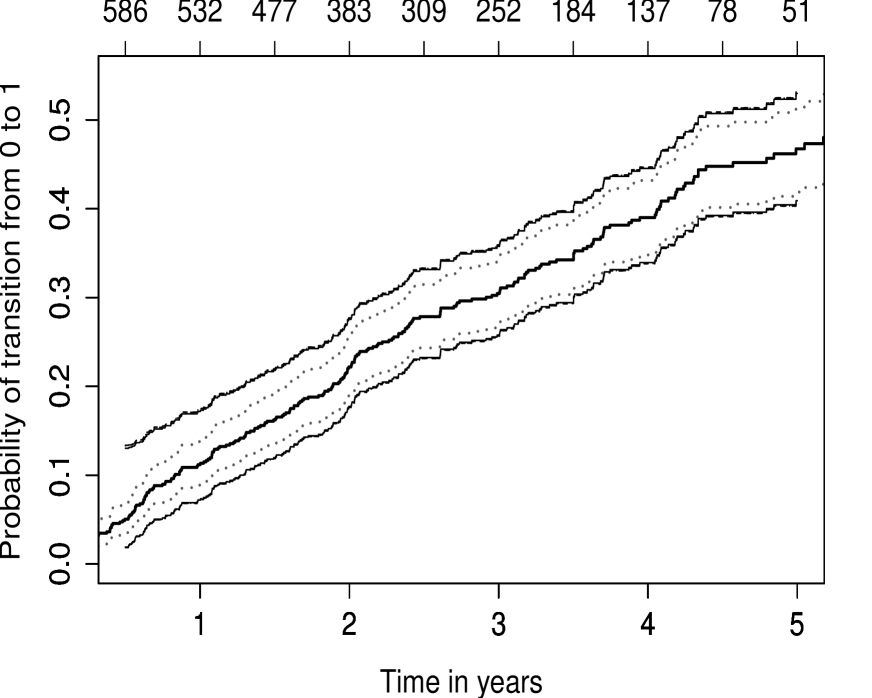
(a) Hall-Wellner bands for $n=636$

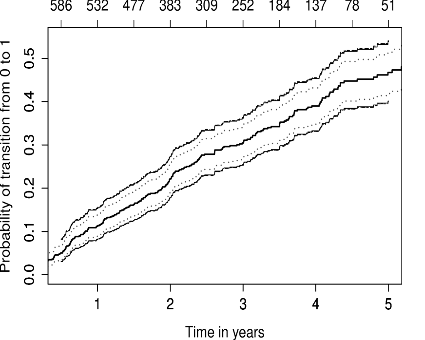
(b) Equal precision bands for $n=636$

Figure 1: Approximate 95% confidence bands for $F_{1}$ using different DDMB weights: standard normal (—-),
centered Poi(1) (- - -), weird bootstrap ($\cdot-\cdot$) multipliers. The solid line in the middle is the corresponding Aalen-Johansen estimator. Pointwise 95% confidence intervals ($\cdots\cdot$) for $F_{1}$ also based on a $\log-\log$ transformation, plotted in dark grey, have been calculated using the R-package etm. Above of the plots the number of individuals under risk shortly before each half-year is indicated.

	Hall-Wellner	Equal precision
normal	.4655	.4621
Poisson	.4783	.4770
weird	.4764	.4746

Table 3: Areas covered by the confidence bands in Figure 1 for different resampling schemes.

We also performed analogous analyses in a data subsample with 200 and 300 individuals. In line with our simulation results, the wild bootstrap with standard normal multipliers produced narrower bands, but - similar to the complete cohort - the differences between the different bands were of little practical importance in this example. In the analyses of the subsample, the bands again performed competetively when compared to pointwise confidence intervals. (Results not shown.)

7 Discussion and Outlook

We have introduced and rigorously justified the new data-dependent multiplier bootstrap for non-parametric analysis of survival data. Observation may be restricted by independent right-censoring and left-truncation, but a strict i.i.d. setup is not required. Our developments have included the case where failure may be due to several competing risks, where resampling is particularly attractive due to lack of asymptotic pivotal approximations. Our general framework includes both the wild bootstrap and the weird bootstrap as special cases. The wild bootstrap with standard normal multipliers is a popular and computationally convenient technique (e.g., Martinussen and Scheike, 2006). The weird bootstrap, introduced by Andersen et al. (1993) in their essential book on Statistical Models Based on Counting Processes, appears to be rarely used, if at all, although it has been implemented in software. To the best of our knowledge, our paper is the first to rigorously show asymptotic correctness of the weird bootstrap in the present context. The variety of available resampling techniques raises the question of which bootstrap to use. Efron’s original proposal of repeatedly taking random samples with replacement from the randomly censored observations (Efron, 1981) is arguably closest to his original approach (Efron, 1979), but does rely on a strict i.i.d. setup; see also the discussion in Andersen et al. (1993, Section IV.1.4). The wild bootstrap with standard normal multipliers is motivated by the martingale representations used in the proofs of weak convergence of the original estimators. In a nutshell, the idea is to replace asymptotic normality by finite sample normality (because of normal multipliers, keeping the data fixed) with approximately the right covariance. The general wild bootstrap allows for non-normal multipliers, replacing finite sample normality by approximate normality. But the weird bootstrap is perhaps the most natural resampling scheme for survival data. To see this, recall that one major reason for basing survival analysis on hazards is censoring. In our setting, and assuming for the time being independent random censorship by $C$, we have that

$$\alpha_{j}(t){\rm d}t=P(T\in[t,t+{\rm d}t),X_{T}=j\,|\,T\geq t)=P(T\in[t,t+{\rm d}t),X_{T}=j,T\leq C\,|\,T\geq t,C\geq t),$$

where the first equality is the definition from Equation (2.1) and the second equality follows because of random censoring. Independent censoring now essentially requires the last equation (reformulated using counting processes and at-risk processes) to hold rather than the existence of a latent censoring time, which is assumed to be stochastically independent of $(T,X_{T})$. It is the second equality that, first of all, motivates the increments of the cause-specific NAE, say ${\rm d}\widehat{A}_{j}(t)={\rm d}N_{j}(t)/Y(t)$. The weird bootstrap continues from this point by sampling $B(Y(t),{\rm d}\widehat{A}_{j}(t))$-distributed increments at the jump times of $N$. The fact that sampling is performed independently at the jump times is justified by the asymptotic distribution of $\sqrt{n}(\widehat{A}_{j}-A_{j})$ having independent increments.

Our simulation results have shown that one should keep alternatives to the wild bootstrap with the almost exclusively used standard normal multipliers in mind. In the scenarios that we have considered, we found a preference for Poisson multipliers and for the weird bootstrap. Beyersmann et al. (2013) who only considered the wild bootstrap also found a preference for Poisson multipliers, but the differences in the present paper were more pronounced. We did not find noticeable differences between the approaches in the real data example, but our analysis illustrated that simultaneous confidence bands may perform competitively when compared to only pointwise confidence intervals. Such bands should be reported more often, because subject matter interest often does lie in survival curves rather than probabilities at fixed time points.

We are currently investigating extensions of the new DDMB approach to multi-state and regression models, see e.g. Lin et al. (2000) or Scheike and Zhang (2003) for a normal multiplier application. In particular, the weird bootstrap naturally extends to these situations.

8 Appendix

The conditional convergence of the finite-dimensional marginal distributions of a linear, resampled process statistic with DDMB weights can be concluded with the following lemma which generalizes Theorem A.1 in Beyersmann et al. (2013). To this end let $\|\cdot\|$ be a norm on $\mathbb{R}^{d}$, $d\in\mathbb{N}$, and define $\widehat{\textbf{S}}_{n}^{D}=\sum_{i=1}^{n}D_{n;i}\bm{\xi}_{n;i}$. In the following let $\mathcal{C}_{n}$ be a $\sigma$-field which contains $\sigma(\bm{\xi}_{n;i}:i=1,\dots,n)$. $\bm{\xi}_{n;i}$ and $D_{n;i}$ are specified in the following lemma.

Lemma 8.1.

Let the triangular array of random variables $(D_{n;i})_{i=1,\dots,n}:\Omega\rightarrow\mathbb{R}^{n}$ with finite second moments and the triangular array of $\mathbb{R}^{d}$-valued random vectors $(\bm{\xi}_{n;i})_{i=1,\dots,n}$ fulfill the following six conditions:

$$\sum_{i=1}^{n}\bm{\xi}_{n;i}\bm{\xi}_{n;i}^{T}\stackrel{{\scriptstyle p}}{{\longrightarrow}}\Gamma,\quad\text{where $\Gamma$ is a positive definite covariance matrix,}$$ (8.1)

$$\max_{i=1,\dots,n}\|\bm{\xi}_{n;i}\|\stackrel{{\scriptstyle p}}{{\longrightarrow}}0,$$ (8.2)

$$\sqrt{n}\max_{i=1,\dots,n}|\mu_{n;i}|:=\sqrt{n}\max_{i=1,\dots,n}|\mathbb{E}[D_{n;i}|\mathcal{C}_{n}]|\stackrel{{\scriptstyle p}}{{\longrightarrow}}0,$$ (8.3)

$$\max_{i=1,\dots,n}|\sigma_{n;i}^{2}-1|:=\max_{i=1,\dots,n}|\textnormal{var}(D_{n;i}|\mathcal{C}_{n})-1|\stackrel{{\scriptstyle p}}{{\longrightarrow}}0\text{ as }n\rightarrow\infty,$$ (8.4)

$$\mathcal{L}(D_{n;i},i=1,\dots,n\;|\;\mathcal{C}_{n})=\bigotimes_{i=1,\dots,n}\mathcal{L}(D_{n;i}\;|\;\mathcal{C}_{n}).$$ (8.5)

In addition, the weights $(D_{n;i})_{i=1,\dots,n}$ may satisfy the Lindeberg condition in probability given $\mathcal{C}_{n}$, that is

$$\sum_{i=1}^{n}\mathbb{E}\Big{[}\frac{(D_{n;i}-\mu_{n;i})^{2}}{\sum_{j=1}^{n}\sigma_{n;j}^{2}}\textnormal{{1}}\Big{(}\frac{(D_{n;i}-\mu_{n;i})^{2}}{\sum_{j=1}^{n}\sigma_{n;j}^{2}}>\varepsilon\Big{)}\Big{|}\mathcal{C}_{n}\Big{]}\stackrel{{\scriptstyle p}}{{\longrightarrow}}0\qquad\text{ for all }\varepsilon>0.$$ (8.6)

Then the conditional weak convergence $\widehat{\textbf{S}}_{n}^{D}\stackrel{{\scriptstyle d}}{{\longrightarrow}}N(0,\Gamma)$ given $\mathcal{C}_{n}$ holds in probability.

Proof. Following the proof in Beyersmann et al. (2013) we only need to show that $\widehat{S}_{n}^{D}$ satisfies the conditional Lindeberg condition for dimension $d=1$. The case for general $d\in\mathbb{N}$ follows from a modified Cramér-Wold Theorem; see (Pauly, 2011, Theorem 4.1) for details. Thus, we calculate

$$\Gamma^{D}_{n}:=\textnormal{var}(\widehat{S}_{n}^{D}|\mathcal{C}_{n})=\sum_{i=1}^{n}\textnormal{var}(D_{n;i}\xi_{n;i}|\mathcal{C}_{n})=\sum_{i=1}^{n}\xi_{n;i}^{2}\sigma_{n;i}^{2}\stackrel{{\scriptstyle p}}{{\longrightarrow}}\Gamma>0$$ (8.7)

by (8.1) and (8.4). Further, we write $\widehat{S}_{n}^{D}=\sum_{i=1}^{n}(D_{n;i}-\mu_{n;i})\xi_{n;i}+\sum_{i=1}^{n}\mu_{n;i}\xi_{n;i}=:S_{n}^{D}+R_{n}^{D}$ of which $R_{n}^{D}$ is asymptotically negligible by Cauchy-Schwarz’ inequality, Conditions (8.1) and (8.3) and Slutzky’s theorem:

$$|R_{n}^{D}|=\Big{|}\sum_{i=1}^{n}\mu_{n;i}\xi_{n;i}\Big{|}\leq\max_{i=1,\dots,n}|\mu_{n;i}|\sum_{i=1}^{n}|\xi_{n;i}|\leq\max_{i=1,\dots,n}|\mu_{n;i}|\sqrt{n}\Big{(}\sum_{i=1}^{n}\xi_{n;i}^{2}\Big{)}^{1/2}\stackrel{{\scriptstyle p}}{{\longrightarrow}}0\cdot\sqrt{\Gamma}.$$

It remains to verify the conditional Lindeberg condition for $S_{n}^{D}$ in probability where we let $\mathbb{E}[D_{n;i}|\mathcal{C}_{n}]=0$ without loss of generality. For this last step we need that $\sum_{i=1}^{n}(\xi^{2}_{n;i}-\Gamma)\sigma_{n;i}^{2}\stackrel{{\scriptstyle p}}{{\longrightarrow}}0$ which can be easily shown using Condition (8.4) and the convergence in (8.7). Thus, it follows that for all $\delta>0$,

$$P\Big{(}-\delta+\Gamma\sum_{j=1}^{n}\sigma_{n;j}^{2}\leq\Gamma^{D}_{n}\leq\delta+\Gamma\sum_{j=1}^{n}\sigma_{n;j}^{2}\Big{)}\stackrel{{\scriptstyle p}}{{\longrightarrow}}1.$$

Now, for all $\delta,\varepsilon,\eta>0$ sufficiently small and $n$ sufficiently large we have

$$(\Gamma^{D}_{n})^{-1}\sum_{i=1}^{n}\mathbb{E}\left[\left.D_{n;i}^{2}\xi_{n;i}^{2}\textbf{1}((D_{n;i}\xi_{n;i})^{2}>\Gamma^{D}_{n}\varepsilon)\right|\mathcal{C}_{n}\right]$$

$$\leq\Big{(}\Gamma\sum_{j=1}^{n}\sigma_{n;j}^{2}-\delta\Big{)}^{-1}\max_{i=1,\dots,n}\xi_{n;i}^{2}\sum_{i=1}^{n}\mathbb{E}\Big{[}D_{n;i}^{2}\textbf{1}\Big{(}(D_{n;i}\xi_{n;i})^{2}>\Big{(}\Gamma\sum_{j=1}^{n}\sigma_{n;j}^{2}-\delta\Big{)}\varepsilon\Big{)}\;\Big{|}\;\mathcal{C}_{n}\Big{]}+o_{p}(1)$$

$$\leq\Big{(}\frac{\Gamma}{2}\sum_{j=1}^{n}\sigma_{n;j}^{2}\Big{)}^{-1}\textbf{1}\big{(}\max_{i=1,\dots,n}|\xi_{n;i}|<\eta\big{)}\eta^{2}\sum_{i=1}^{n}\mathbb{E}\Big{[}D_{n;i}^{2}\textbf{1}\Big{(}\eta^{2}D_{n;i}^{2}>\Big{(}\frac{\Gamma}{2}\sum_{j=1}^{n}\sigma_{n;j}^{2}\Big{)}\varepsilon\Big{)}\;\Big{|}\;\mathcal{C}_{n}\Big{]}+o_{p}(1)$$

which is $o_{p}(1)$ by (8.6). Therefore, $\widehat{S}_{n}^{D}$ satisfies the Lindeberg condition given $\mathcal{C}_{n}$ in probability. $\Box$

Remark 3.

See Beyersmann et al. (2013) to note that Conditions (8.1) and (8.2) are fulfilled for the triangular array $\bm{\xi}_{n}=\sqrt{\frac{n_{1}n_{2}}{n}}(\textbf{Z}_{2n}^{(k)}(t_{j}))_{j,k}$ and $\mathcal{C}_{n}=\mathcal{A}_{n}$ where, for each $j=1,\dots,\ell,k=1,2,$ the vector $\textbf{Z}_{2n}^{(k)}(t_{j})=(Z_{2n;1}^{(k)}(t_{j}),\dots,Z_{2n;2n_{k}}^{(k)}(t_{j}))$ consists of the integrals w.r.t. counting processes given by (3.1) and (4.2) evaluated at arbitrary times $t_{1},\dots,t_{\ell}\in I$. Moreover, this choice for $\bm{\xi}_{n}$ also fulfills the conditions of Lemma 8.2 below.

Let us now give a criterion for the tightness of linear, resampled process statistics in terms of the DDMB weights $(D_{n;i})_{i=1,\dots,n}$ and the data vectors $(\bm{\xi}_{n;i})_{i=1,\dots,n}$. Since tightness of a family of multivariate processes is equivalent to the tightness in each dimension, we here only consider the case of $d=1$. Recall the $\mathcal{O}_{p}$-notation introduced above Theorem 1.

Lemma 8.2.

Let each $\xi_{n;i}:\Omega\times I\rightarrow\mathbb{R},i=1,\dots,n,$ be a stochastic process and suppose that, as $n\rightarrow\infty$,

$$\max_{i=1,\dots,n}|\mathbb{E}[D_{n;i}|\mathcal{C}_{n}]|\in\mathcal{O}_{p}(n^{-1/2}),$$ (8.8)

$$\max_{i=1,\dots,n}\mathbb{E}[D^{2}_{n;i}|\mathcal{C}_{n}]\in\mathcal{O}_{p}(1),$$ (8.9)

$$\max_{i=1,\dots,n}|\mathbb{E}[D^{3}_{n;i}|\mathcal{C}_{n}]|\in\mathcal{O}_{p}(\sqrt{n/r_{n}}),$$ (8.10)

$$\max_{i=1,\dots,n}\mathbb{E}[D^{4}_{n;i}|\mathcal{C}_{n}]\in\mathcal{O}_{p}(r_{n}^{-1}),$$ (8.11)

$$\mathcal{L}(D_{n;i},i=1,\dots,n\;|\;\mathcal{C}_{n})=\bigotimes_{i=1,\dots,n}\mathcal{L}(D_{n;i}\;|\;\mathcal{C}_{n}),$$ (8.12)

$$\sum_{i=1}^{n}(\xi_{n;i}(s)-\xi_{n;i}(r))^{2}\leq H_{n}(s)-H_{n}(r)\stackrel{{\scriptstyle p}}{{\longrightarrow}}H(s)-H(r),\quad 0\leq r\leq s,\;r,s\in I,$$ (8.13)

where $H,H_{n}:\Omega\times I\rightarrow[0,\infty)$ are nondecreasing functions of which $H$ is continuous and deterministic and where $r_{n}=\max_{i=1,\dots,n}\max_{s,t\in I}\frac{(\xi_{n;i}(t)-\xi_{n;i}(s))^{2}}{\sum_{j=1}^{n}(\xi_{n;j}(t)-\xi_{n;j}(s))^{2}}\in(0,1)$. Then the family of probability measures $\mathcal{L}\big{(}\widehat{S}_{n}^{D}|\mathcal{C}_{n}\big{)}$ is tight in probability.

Proof.

By its analogy to the proof of tightness for the exchangeably weighted bootstrapped Aalen-Johansen process in Dobler and Pauly (2014), where the moment conditions for the (mixed) moments are now replaced by (8.8) – (8.12), we only need to consider the asymptotics of the involved moments therein; see the proof of their Theorem 3.1. In fact, moving on to the conditional expectations essentially does not effect the arguments of the referred proof. It is sufficient to verify that the existing proof holds with these modifications.

Note that we here analyze the conditional moments of $\widehat{S}_{n}^{D}$ without previously centering the DDMB weights at their arithmetic mean which had been necessary in the article by Dobler and Pauly (2014).

Two of those five cases emerging in the referred proof require a separate consideration since our Lemma 8.2 is formulated in a greater generality. Therefore, we begin to note that, in the first sum on the right-hand side of (A.3) in Dobler and Pauly (2014), where $\mathbb{E}[D^{4}_{n;i}|\mathcal{C}_{n}]$ occurs, we also have factors like

$$\sum_{i=1}^{n}(\xi_{n;i}(t)-\xi_{n;i}(s))^{2}(\xi_{n;i}(s)-\xi_{n;i}(r))^{2}$$

$$=\sum_{i=1}^{n}\frac{(\xi_{n;i}(t)-\xi_{n;i}(s))^{2}}{\sum_{j=1}^{n}(\xi_{n;j}(t)-\xi_{n;j}(s))^{2}}(\xi_{n;i}(s)-\xi_{n;i}(r))^{2}\sum_{j=1}^{n}(\xi_{n;j}(t)-\xi_{n;j}(s))^{2}$$

$$\leq r_{n}\sum_{j=1}^{n}(\xi_{n;j}(t)-\xi_{n;j}(s))^{2}\sum_{i=1}^{n}(\xi_{n;i}(s)-\xi_{n;i}(r))^{2}.$$

This is why (8.11) is sufficient for having reasonable upper bounds of this first sum. A similar argument is required for those sums where third moments occur, i.e.,

$$\sum_{i=1}^{n}(\xi_{n;i}(t)-\xi_{n;i}(s))(\xi_{n;i}(s)-\xi_{n;i}(r))^{2}$$

$$=\sum_{i=1}^{n}\frac{(\xi_{n;i}(t)-\xi_{n;i}(s))}{(\sum_{j=1}^{n}(\xi_{n;j}(t)-\xi_{n;j}(s))^{2})^{1/2}}(\xi_{n;i}(s)-\xi_{n;i}(r))^{2}\Big{(}\sum_{j=1}^{n}(\xi_{n;j}(t)-\xi_{n;j}(s))^{2}\Big{)}^{1/2}$$

$$\leq\sqrt{r_{n}}\Big{(}\sum_{j=1}^{n}(\xi_{n;j}(t)-\xi_{n;j}(s))^{2}\Big{)}^{1/2}\sum_{k=1}^{n}(\xi_{n;k}(s)-\xi_{n;k}(r))^{2}.$$

Hence, Conditions (8.8) and (8.10) are sufficient for bounds of these sums. It remains to inspect

$$\max_{i\neq j}\mathbb{E}[D^{2}_{n;i}D^{2}_{n;j}|\mathcal{C}_{n}]\leq \max_{i=1,\dots,n}\mathbb{E}[D^{2}_{n;i}|\mathcal{C}_{n}]^{2}\in\mathcal{O}_{p}(1),$$

$$n\max_{i\neq j\neq k\neq i}|\mathbb{E}[D^{2}_{n;i}D_{n;j}D_{n;k}|\mathcal{C}_{n}]|\leq \max_{i,j=1,\dots,n}\mathbb{E}[D^{2}_{n;i}|\mathcal{C}_{n}]n\mathbb{E}[D_{n;j}|\mathcal{C}_{n}]^{2}\in\mathcal{O}_{p}(1),$$

$$n^{2}\max_{i,j,k,l\text{ pairwise different}}|\mathbb{E}[D_{n;i}D_{n;j}D_{n;k}D_{n;l}|\mathcal{C}_{n}]|\leq \max_{i=1,\dots,n}(\sqrt{n}\mathbb{E}[D_{n;i}|\mathcal{C}_{n}])^{4}\in\mathcal{O}_{p}(1).$$

It is also worth to mention that in fact a modified version of Billingsley (1999), Theorem 13.5, is applied here such that the non-decreasing function therein may be replaced with a sequence of non-decreasing functions converging pointwise to a continuous one; see the remark in Jacod and Shiryaev (2003), p. 356. Since we are considering conditional expectations, this condition was translated into the convergence in probability in (8.13) by applying the subsequence principle. $\Box$

Proof of Theorem 1.

The result follows from Lemmas 8.1 and 8.2 taken into account Remark 3 and the calculations in the proof of Theorem 2 in Beyersmann et al. (2013) to see that $nr_{n}\in\mathcal{O}_{p}(1)$. Also, note that the condition

$$\max_{1\leq i\leq 2n}|\mathbb{E}[D^{3}_{2n;i}|\mathcal{A}_{n}]|\in\mathcal{O}_{p}(n)$$

is already fulfilled by (3.5) in combination with Jensen’s inequality applied with $g:x\mapsto x^{4/3}$. $\Box$

Proof of Example 1.

Only (d) needs to be proven. The other examples are obviously special cases of the proposed DDMB of Theorem 1. For the weird bootstrap, the limits of conditional mean and variance are given as

$$\sqrt{n}|\mathbb{E}\left[\left.B_{i}\right|\mathcal{A}_{n}\right]|=\sqrt{n}\Big{(}1-Y(\tilde{T}_{i})\frac{1}{Y(\tilde{T}_{i})}\Big{)}=0$$

and $$|\textnormal{var}(B_{i}|\mathcal{A}_{n})-1|=\Big{|}Y(\tilde{T}_{i})\frac{1}{Y(\tilde{T}_{i})}\Big{(}1-\frac{1}{Y(\tilde{T}_{i})}\Big{)}-1\Big{|}\leq\sup_{s\in[0,t]}\frac{1}{Y(s)}\stackrel{{\scriptstyle p}}{{\longrightarrow}}0$$

and the convergence is due to Condition (2.7). Obviously, the Lyapunov condition in Remark 1(a) holds too and (3.6) holds per definition of the $B_{i}$. Thus, we have shown that (3.3) – (3.7) are fulfilled. $\Box$

References

- Aalen et al. (2008) O. O. Aalen, Ø. Borgan, and H. K. Gjessing. Survival and Event History Analysis: A Process Point of View. Springer Science & Business Media, 2008.
- Akritas (1986) M. G. Akritas. Bootstrapping the Kaplan-Meier Estimator. Journal of the American Statistical Association, 81(396):1032–1038, 1986.
- Allignol et al. (2010) A. Allignol, M. Schumacher, and J. Beyersmann. A note on variance estimation of the Aalen-Johansen estimator of the cumulative incidence function in competing risks, with a view towards left-truncated data. Biom. J., 52(1):126–137, 2010.
- Allignol et al. (2011) A. Allignol, M. Schumacher, C. Wanner, C. Drechsler, and J. Beyersmann. Understanding competing risks: a simulation point of view. BMC Medical Research Methodology, 11:86, 2011.
- Andersen et al. (1993) P. K. Andersen, Ø. Borgan, R. D. Gill, and N. Keiding. Statistical Models Based on Counting Processes. Springer, New York, 1993.
- Bajorunaite and Klein (2007) R. Bajorunaite and J. P. Klein. Two-sample tests of the equality of two cumulative incidence functions. Computational Statistics Data Analysis, 51:4269–4281, 2007.
- Bajorunaite and Klein (2008) R. Bajorunaite and J. P. Klein. Comparison of failure probabilities in the presence of competing risks. J. Stat. Comput. Simul., 78:951–966, 2008.
- Beyersmann et al. (2012) J. Beyersmann, A. Allignol, and M. Schumacher. Competing risks and multistate models with R. Springer, New York, 2012.
- Beyersmann et al. (2013) J. Beyersmann, M. Pauly, and S. Di Termini. Weak Convergence of the Wild Bootstrap for the Aalen-Johansen Estimator of the Cumulative Incidence Function of a Competing Risk. Scandinavian Journal of Statistics, 2013.
- Billingsley (1999) P. Billingsley. Convergence of probability measures. Wiley, New York, second edition, 1999.
- Broström (2012) G. Broström. Event History Analysis with R. CRC Press, 2012.
- Davison and Hinkley (1997) A. C. Davison and D. V. Hinkley. Bootstrap Methods and their Applications. Cambridge University Press Cambridge, first edition, 1997.
- Dobler and Pauly (2014) D. Dobler and M. Pauly. Bootstrapping Aalen-Johansen processes for competing risks: Handicaps, solutions, and limitations. Electronic Journal of Statistics, 8:2779–2803, 2014.
- Dobler and Pauly (2015) D. Dobler and M Pauly. Approximative Tests for the Equality of two Cumulative Incidence Functions of a Competing Risk. preprint arXiv:1402.2209, 2015.
- Doss and Gill (1992) H. Doss and R. D. Gill. An Elementary Approach to Weak Convergence for Quantile Processes, with Applications to Censored Survival Data. Journal of the American Statistical Association, 87(419):869–877, 1992.
- Dudek et al. (2008) A. Dudek, M. Goćwin, and J. Leśkow. Simultaneous confidence bands for the integrated hazard function. Computational Statistics, 23(1):41–62, 2008. ISSN 0943-4062.
- Efron (1979) B. Efron. Bootstrap methods: another look at the jackknife. Ann. Statist., 7(1):1–26, 1979. ISSN 0090-5364.
- Efron (1981) B. Efron. Censored Data and the Bootstrap. Journal of the American Statistical Association, 76(374):312–319, 1981.
- Fledelius et al. (2004) P. Fledelius, M. Guillen, J. P. Nielsen, and M. Vogelius. Two-dimensional Hazard Estimation for Longevity Analysis. Scandinavian Actuarial Journal, 2004(2):133–156, 2004.
- Freitag (2000) G. Freitag. Validierung von Modellen in der Überlebenszeitanalyse. PhD thesis, Ruhr-Universität Bochum, 2000.
- Jacod and Shiryaev (2003) J. Jacod and A. N. Shiryaev. Limit Theorems for Stochastic Processes. Springer, Berlin, second edition, 2003.
- Lin (1994) D. Y. Lin. Cox regression analysis of multivariate failure time data: the marginal approach. Statistics in Medicine, 13(21):2233–2247, 1994.
- Lin (1997) D. Y. Lin. Non-parametric inference for cumulative incidence functions in competing risks studies. Statistics and Medicine, 16:901–910, 1997.
- Lin et al. (1993) D. Y. Lin, L. J. Wei, and Z. Ying. Checking the Cox model with cumulative sums of martingale-based residuals. Biometrika, 80(3):557–572, 1993.
- Lin et al. (2000) D. Y. Lin, L. J. Wei, I. Yang, and Z. Ying. Semiparametric regression for the mean and rate functions of recurrent events. Journal of the Royal Statistical Society. Series B, Statistical Methodology, pages 711–730, 2000.
- Lo and Singh (1986) S.-H. Lo and K. Singh. The Product-Limit Estimator and the Bootstrap: Some Asymptotic Representations. Probability Theory and Related Fields, 71(3):455–465, 1986.
- Martinussen and Scheike (2006) T. Martinussen and T. H. Scheike. Dynamic Regression Models for Survival Data. New York, NY: Springer, 2006.
- Pauly (2011) M. Pauly. Weighted resampling of martingale difference arrays with applications. Electronic Journal of Statistics, 5:41–52, 2011.
- Scheike and Zhang (2003) T. H. Scheike and M.-J. Zhang. Extensions and applications of the cox-aalen survival model. Biometrics, 59(4):1036–1045, 2003.
- Schulgen et al. (2005) G. Schulgen, M. Olschewski, V. Krane, C. Wanner, G. Ruf, and M. Schumacher. Sample sizes for clinical trials with time-to-event endpoints and competing risks. Contemporary Clinical Trials, 26:386–395, 2005.
- Wanner et al. (2005) C. Wanner, V. Krane, W. März, M. Olschewski, J. F. E. Mann, G. Ruf, and E. Ritz. Atorvastatin in Patients with Type 2 Diabetes Mellitus Undergoing Hemodialysis. New England Journal of Medicine, 353(3):238–248, 2005.