Non-Hermitian propagation of Hagedorn wavepackets

Abstract

We investigate the time evolution of Hagedorn wavepackets by non-Hermitian quadratic Hamiltonians. We state a direct connection between coherent states and Lagrangian frames. For the time evolution a multivariate polynomial recursion is derived that describes the activation of lower lying excited states, a phenomenon unprecedented for Hermitian propagation. Finally we apply the propagation of excited states to the Davies–Swanson oscillator.

Keywords: non-Hermitian dynamics, Hagedorn wavepackets, complex Lagrangian subspaces, ladder operators

Mathematics Subject Classification: 42C05, 81Q12, 81S10

1 Introduction

In the last two decades considerable interest in non-selfadjoint operators has developed, and even the simplest examples have provided phenomena that greatly differ from what is established in the familiar Hermitian context. This pronounced deviation is at the core of the theory of quantum physical resonances [Moi11] and has strongly motivated the research on the pseudospectrum of non-selfadjoint operators [TE05]. Our investigation of non-Hermiticity will concentrate on the initial value problem

$$\mathrm{i}\varepsilon\partial_{t}\psi(t)=\operatorname{Op}[{\mathcal{H}}_{t}]\psi(t)\ ,\qquad\psi(0)=\psi_{0}\ ,$$ (1.1)

where $\varepsilon>0$ is a fixed positive parameter, $\psi_{0}\in L^{2}(\mathds{R}^{n})$, and $\operatorname{Op}[{\mathcal{H}}_{t}]$ is the Weyl quantised operator of the quadratic function

$${\mathcal{H}}_{t}(z)=\tfrac{1}{2}z\cdot H_{t}z\ ,\qquad z\in\mathds{R}^{2n}\ ,$$

associated with a possibly time-dependent complex symmetric matrix $H_{t}\in\mathds{C}^{2n\times 2n}$. This seemingly simple model problem already encorporates several non-Hermitian challenges and clearly hints at the behaviour of more general systems in the semiclassical limit $\varepsilon\to 0$.

So far, non-Hermitian harmonic systems have been mostly analysed from the spectral point of view or in the context of $\mathcal{P}T$ symmetry, see for example [Sjö74, §3],[Dav99b] or more recently [CGHS12, KSTV15]. It has been proven that the condition number of the eigenvalues of non-Hermitian harmonic systems grows rapidly with respect to their size [DK04, Hen14], while spectral asymptotics have been obtained for skew-symmetric perturbations of harmonic oscillators as well as for non-selfadjoint system with double characteristics [GGN09, HP13, HSV13]. The semigroup of non-selfadjoint quadratic operators has been analysed in [Pra08] and [AV15, Vio16]. A complementary line of research [GS11, GS12] has emphasised the new, unexpected geometrical structures that emerge for the non-Hermitian propagation of Gaussian coherent states. Our aim here is to extend these geometrical findings to the larger class of Hagedorn wavepackets and to add the explicit description of additional non-Hermitian signatures of the dynamics.

Over decades, the Hermitian time evolution of Gaussian and Hagedorn wavepackets has evolved into a very versatile tool with wide-ranging application in many areas. It was realised by Hepp and Heller [Hep74, Hel75, Hel76] that in order to compute the propagation in the semiclassical limit one only needs one classical trajectory $t\mapsto z_{t}$ through the centre of the wavepacket and the linearisation of the classical flow around it,

$$\dot{S}_{t}=\Omega D^{2}{\mathcal{H}}_{t}(z_{t})S_{t}\ ,\qquad S_{t}\in\mathds{C}^{2n\times 2n}\ ,\qquad\Omega=\begin{pmatrix}0&-\mathrm{Id}_{n}\\ \mathrm{Id}_{n}&0\end{pmatrix}\ ,$$

where $D^{2}{\mathcal{H}}_{t}(z_{t})$ denotes the Hessian matrix of ${\mathcal{H}}_{t}$ evaluated in $z_{t}$. This method was widely used in applications, in particular in chemistry [Lit86, YU00]. More recently Gaussian wavepackets have been more systematically used as a tool for the numerical analysis of highly oscillatory initial value problems, either within the wide framework of Gaussian beams methods, see for example [LRT13], or for Hermitian quantum dynamics with Hagedorn wavepackets [Lub08, GH14]. Let us give a brief overview of the concepts we develop in this work.

A Gaussian coherent state is parametrised by a phase space point $z_{0}\in\mathds{R}^{2n}$ and a normalised Lagrangian frame, that is a rectangular matrix $Z_{0}\in\mathds{C}^{2n\times n}$ satisfying the conditions

$$Z_{0}^{T}\Omega Z_{0}=0\quad\text{and}\quad\tfrac{1}{2\mathrm{i}}\,Z_{0}^{*}\Omega Z_{0}=\mathrm{Id}_{n}\ .$$ (1.2)

Assuming $z_{0}=0$ for the ease of notation, we introduce the associated lowering operator

$${A(Z_{0})=\frac{\mathrm{i}}{\sqrt{2\varepsilon}}Z_{0}^{T}\Omega\hat{z}}\ ,\qquad\hat{z}=\begin{pmatrix}-\mathrm{i}\varepsilon\nabla_{x}\\ x\end{pmatrix}\ ,$$

and the raising operator

$$A^{\dagger}(Z_{0})=-A(\bar{Z}_{0})$$

as its formal adjoint, where $\bar{Z}_{0}$ denotes the complex conjugate of the matrix $Z_{0}$. The wavepacket $\varphi_{0}(Z_{0})$ is defined as an element in the kernel of the lowering operator $A(Z_{0})$, i.e. by $A(Z_{0})\varphi_{0}(Z_{0})=0$, and it is normalised according to

$$\|\varphi_{0}(Z_{0})\|^{2}=\int_{\mathds{R}^{n}}|\varphi_{0}(Z_{0})(x)|^{2}dx=1.$$

This determines $\varphi_{0}(Z_{0})$ up to a phase factor. The Gaussian wavepacket $\varphi_{0}(Z_{0})$ is the zeroth element of an orthonormal basis of $L^{2}(\mathds{R}^{n})$ constructed by the repeated application of the components of the raising operator to the coherent state. The definition

$$\varphi_{\alpha}(Z_{0})=\frac{1}{\sqrt{\alpha!}}A^{\dagger}(Z)^{\alpha}\varphi_{0}(Z_{0})\ ,\qquad\alpha\in\mathds{N}_{0}^{n}\ ,$$

is due to Hagedorn [Hag98], who called the basis elements semiclassical wavepackets, simplifying his earlier construction that was based on a less transparent polynomial recursion [Hag85]. The generalised coherent states [CR12, §4.1], that are obtained by applying a unitary squeezing transformation to the $n$-fold product of univariate harmonic oscillator eigenfunctions, only differ by a phase factor from the semiclassical wavepackets. For our study of non-Hermitian dynamics we follow Hagedorn’s ladder approach and use the time evolution of both the raising and lowering operators to explicitly describe the propagation of the basis functions.

We concern the propagation of an excited initial wavepacket

$$\psi(0)=\varphi_{\alpha}(Z_{0})\ ,\qquad\alpha\in\mathds{N}_{0}^{n}\ .$$

In the Hermitian situation the evolution is simply given by $\psi(t)=\varphi_{\alpha}(S_{t}Z_{0})$ where the flow matrix $S_{t}\in{\rm Sp}(n,\mathds{R})$ is real symplectic, and $S_{t}Z_{0}$ is a normalised Lagrangian frame for all times $t\in\mathds{R}$. In the non-Hermitian case, $S_{t}\in{\rm Sp}(n,\mathds{C})$ is a complex symplectic matrix, and we have to expect that

$$S_{t}^{*}\Omega S_{t}\neq\Omega.$$

In particular, the rectangular matrix $S_{t}Z_{0}$ violates the second, normalising, condition of (1.2), and we have to restrict our analysis to time intervals $[0,T[$ such that

$$\tfrac{1}{2\mathrm{i}}(S_{t}Z_{0})^{*}\Omega(S_{t}Z_{0})>0,\qquad t\in[0,T[\ .$$

We use the Hermitian, positive definite matrix

$$N_{t}:=\left(\tfrac{1}{2\mathrm{i}}(S_{t}Z_{0})^{*}\Omega(S_{t}Z_{0})\right)^{-1/2}$$

to construct a normalised Lagrangian frame $Z_{t}:=S_{t}Z_{0}N_{t}$ with the same range as $S_{t}Z_{0}$. We then obtain that for an initial coherent state $\psi(0)=\varphi_{0}(Z_{0})$, the corresponding solution of the initial value problem (1.1) is of the form

$$\psi(t)=\mathrm{e}^{\beta_{t}}\varphi_{0}(Z_{t})$$

with $\|\varphi_{0}(Z_{t})\|=1$, where the real-valued gain or loss parameter

$$\beta_{t}=\tfrac{1}{4}\int_{0}^{t}\operatorname{tr}(G_{\tau}^{-1}\operatorname{Im}H_{\tau})d\tau$$

is determined by the symplectic metric $G_{t}=\Omega^{T}\operatorname{Re}(Z_{t}Z_{t}^{*})\Omega\in\mathrm{Sp}(n,\mathds{R})$ associated with the normalised Lagrangian frame $Z_{t}$, see also [GS12, §3]. Our main new result states the expansion of the time-evolved wavepacket $\psi(t)$ with respect to the orthonormal basis $\varphi_{k}(Z_{t})$, $k\in\mathds{N}_{0}^{n}$, that is parametrised by the normalised Lagrangian frame $Z_{t}$.

For non-Hermitian dynamics, however, the propagated excited states are utterly different. The two Lagrangian frames $S_{t}Z_{0}$ and $\bar{S}_{t}Z_{0}$ do not only lose normalisation but also have different ranges. Therefore, the dynamics also activate lower lying excited states and we obtain

$$\psi(t)=\mathrm{e}^{\beta_{t}}\sum_{|k|\leq|\alpha|}a_{k}(t)\varphi_{k}(Z_{t})\ ,\qquad t\in[0,T[\ ,$$

with expansion coefficients $a_{k}(t)\in\mathds{C}$ for $|k|\leq|\alpha|$. These coefficients can be explicitly inferred from Theorem 4.5, that proves

$$\psi(t)=\frac{\mathrm{e}^{\beta_{t}}}{\sqrt{\alpha!}}\,q_{\alpha}({N_{t}}A^{\dagger}(Z_{t}))\varphi_{0}(Z_{t})\ ,$$

where the multivariate polynomials $q_{\alpha}$ satisfy the recursion relation

$$q_{0}(x)=1\ ,\qquad q_{\alpha+e_{j}}(x)=x_{j}q_{\alpha}(x)-e_{j}\cdot M_{t}\nabla q_{\alpha}(x)\ ,\qquad j=1,\ldots,n\ .$$

The complex symmetric matrix

$${M_{t}=\tfrac{1}{4}(S_{t}\bar{Z}_{0})^{T}G_{t}(S_{t}\bar{Z}_{0})}\in\mathds{C}^{n\times n}$$

governing the recursion is determined by the symplectic metric $G_{t}$ and the complex flow $S_{t}$. In general, the complex symmetric $M_{t}$ does not have a specific sparsity pattern so that all the $n$ dimensions are coupled within the polynomial recursion.

We have organised the paper as follows: Section 2 develops the symplectic linear algebra of complex Lagrangian subspaces required for the parametrisation of the Hagedorn wavepackets. Section 3 constructs coherent states, ladder operators and Hagedorn wavepackets parametrised by positive Lagrangian frames. Section 4 is the core of our manuscript. It analyses the non-Hermitian time evolution of Hagedorn wavepackets, and in particular proves our main result Theorem 4.5. Section 5 illustrates our results for the one-dimensional Davies–Swanson oscillator and the heat equation. The four appendices summarise elementary facts on Weyl calculus, present a proof of the Riccati equation for the symplectic metric $G_{t}$, and discuss basic properties of the multivariate polynomials $q_{\alpha}$, $\alpha\in\mathds{N}_{0}^{n}$ and the wavepackets in one and two dimensions.

2 Lagrangian subspaces

We start by discussing some symplectic linear algebra with a focus on complex vector spaces and complex matrices. We endow the real vector space $\mathds{R}^{2n}$ with the standard symplectic form $\mathds{R}^{2n}\times\mathds{R}^{2n}\to\mathds{R}$, $(x,y)\mapsto x\cdot\Omega y$, using the invertible skew-symmetric matrix

$$\Omega=\begin{pmatrix}0&-\mathrm{Id}_{n}\\ \mathrm{Id}_{n}&0\end{pmatrix}\in\mathds{R}^{2n\times 2n}\ .$$

Matrices $S\in\mathds{R}^{2n\times 2n}$ respecting the standard symplectic structure satisfy $S^{T}\Omega S=\Omega$ and consequently $S^{-1}=\Omega^{T}S^{T}\Omega$. They are called symplectic and constitute the symplectic group $\mathrm{Sp}(n,\mathds{R})$, see also [MS98, §I.2]. Writing a symplectic matrix as $S=(U,V)$ with $U,V\in\mathds{R}^{2n\times n}$, the complex rectangular matrix $Z=U-\mathrm{i}V\in\mathds{C}^{2n\times n}$ satisfies

$$Z^{T}\Omega Z=0\ ,\qquad Z^{*}\Omega Z=2\mathrm{i}\mathrm{Id}_{n}\ ,$$ (2.1)

where $Z^{*}=\overline{Z}^{T}$ denotes the Hermitian adjoint. We see from the first property of $Z$ that all vectors $l,l^{\prime}\in\operatorname{range}Z$ satisfy

$$l\cdot\Omega l^{\prime}=0\ .$$

Such vectors are called skew-orthogonal, and a subspace $L\subset\mathds{C}^{n}\oplus\mathds{C}^{n}$ is called isotropic, if all vectors in $L$ are skew-orthogonal to each other. Moreover, $L$ is called Lagrangian, if it is isotropic and has dimension $n$, which is the maximal dimension an isotropic subspace can have (by the non-degeneracy of $\Omega$). From the second property of the matrix $Z$, we see that all vectors $l\in\operatorname{range}Z\setminus\{0\}$ satisfy

$$\tfrac{\mathrm{i}}{2}(\Omega\bar{l})\cdot l>0\ .$$

That is, the quadratic form

$$h(z,z^{\prime}):=\tfrac{\mathrm{i}}{2}(\Omega\bar{z})\cdot z^{\prime}=\tfrac{\mathrm{i}}{2}\bar{z}\cdot\Omega^{T}z^{\prime},\qquad z,z^{\prime}\in\mathds{C}^{n}\oplus\mathds{C}^{n}\ ,$$

is positive on $\operatorname{range}Z$. Such a Lagrangian subspace is called positive.

Remark 2.1.

In the literature, [Lub08], the choice $Z=U+iV$ is more common, but for our purposes the complex conjugate is more natural, since it matches with Hagedorn’s notation, [Hag98]. However, the main results hold true for both definitions.

2.1 Lagrangian frames

Rectangular matrices satisfying conditions (2.1) are convenient tools when working with Lagrangian subspaces. In particular, the normalisation condition $Z^{*}\Omega Z=2\mathrm{i}\mathrm{Id}_{n}$ will be crucial later on when studying the effects of non-Hermitian dynamics.

Definition 2.2 (Lagrangian frame).

We say that a matrix $Z\in\mathds{C}^{2n\times n}$ is isotropic, if

$$Z^{T}\Omega Z=0\ ,$$

and it is called normalised, if

$$Z^{*}\Omega Z=2\mathrm{i}\mathrm{Id}_{n}\ .$$

An isotropic matrix of rank $n$ is called a Lagrangian frame.

As indicated before, normalised Lagrangian frames are in one-to-one correspondence with symplectic matrices: Writing $S\in\mathrm{Sp}(n,\mathds{R})$ as $S=(U,V)$ with $U,V\in\mathds{R}^{2n\times n}$, then $Z=U-\mathrm{i}V$ is isotropic and normalised. Vice versa, if $Z\in\mathds{C}^{2n\times n}$ is a normalised Lagrangian frame, then $S=(\operatorname{Re}(Z),-\operatorname{Im}(Z))$ is symplectic. For a positive Lagrangian subspace $L\subset\mathds{C}^{n}\oplus\mathds{C}^{n}$ there are plenty of normalised Lagrangian frames spanning $L$. Denoting by

$$F_{\rm n}(L)=\left\{Z\in\mathds{C}^{2n\times n};\;\operatorname{range}Z=L,Z^{*}\Omega Z=2\mathrm{i}\mathrm{Id}_{n}\right\}$$

the set of normalised Lagrangian frames spanning $L$, we observe that all its elements are related by unitary transformations. Indeed, since any $Z_{0},Z_{1}\in F_{\rm n}(L)$ have the same range, there exists an invertible matrix $C\in\mathds{C}^{n\times n}$ so that $Z_{1}=Z_{0}C$, and the normalisation requires that $C$ is unitary.

2.2 Orthogonal projections

The complex conjugate $\bar{L}$ of a positive Lagrangian subspace $L\subset\mathds{C}^{n}\oplus\mathds{C}^{n}$ is Lagrangian, too, and all vectors $l\in\bar{L}\setminus\{0\}$ satisfy

$$h(l,l)=\tfrac{\mathrm{i}}{2}\bar{l}\cdot\Omega^{T}l<0\ ,$$

so that $\bar{L}$ is called a negative Lagrangian. It is clear that $L\cap\bar{L}=\{0\}$, because if $l\in L\cap\bar{L}$, then $l$ is real, and hence $h(l,l)=\mathrm{i}l\cdot\Omega l/2=0$, so that $l=0$. Therefore,

$$\mathds{C}^{n}\oplus\mathds{C}^{n}=L\oplus\bar{L}\ .$$

This decomposition of $\mathds{C}^{n}\oplus\mathds{C}^{n}$ is orthogonal in the sense that

$$h(l,l^{\prime})=0\quad\mbox{for all}\quad l\in L,l^{\prime}\in\bar{L}\ .$$

Proposition 2.3 (Projections).

Let $L\subset\mathds{C}^{n}\oplus\mathds{C}^{n}$ be a positive Lagrangian and $Z\in F_{\rm n}(L)$. Then,

$$\pi_{L}=\tfrac{\mathrm{i}}{2}ZZ^{*}\Omega^{T}\quad\mbox{and}\quad\pi_{\bar{L}}=-\tfrac{\mathrm{i}}{2}\bar{Z}Z^{T}\Omega^{T}$$

are the orthogonal projections onto $L$ and $\bar{L}$, respectively, that is,

• $\pi_{L}\mid_{L}=\mathrm{Id}_{2n}$, $\pi_{L}\mid_{\bar{L}}=0$ and $\pi_{\bar{L}}\mid_{\bar{L}}=\mathrm{Id}_{2n}$, $\pi_{\bar{L}}\mid_{L}=0$  ,

• $\pi_{L}^{2}=\pi_{L}$ and $\pi_{\bar{L}}^{2}=\pi_{\bar{L}}$  ,

• $h(\pi_{L}z,z^{\prime})=h(z,\pi_{L}z^{\prime})$ and $h(\pi_{\bar{L}}z,z^{\prime})=h(z,\pi_{\bar{L}}z^{\prime})$ for all $z,z^{\prime}\in\mathds{C}^{n}\oplus\mathds{C}^{n}$  ,

Proof.

To prove $\pi_{L}\mid_{L}=\mathrm{Id}_{2n}$ and $\pi_{L}\mid_{\bar{L}}=0$, we observe

$$\pi_{L}Z=\tfrac{\mathrm{i}}{2}ZZ^{*}\Omega^{T}Z=Z\ ,\qquad\pi_{L}\bar{Z}=\tfrac{\mathrm{i}}{2}ZZ^{*}\Omega^{T}\bar{Z}=0\ .$$

The other properties of $\pi_{L}$ and $\pi_{\bar{L}}$ are also proved by short calculations using that $Z$ is isotropic and normalised. ∎

2.3 Siegel half space

A large set of Lagrangian subspaces can be naturally parametrised by complex symmetric matrices. If the Lagrangian is positive or negative, then we encounter complex symmetric matrices with positive or negative definite imaginary part, that is, elements of the upper or lower Siegel half space.

Lemma 2.4 (Siegel half space).

Assume that $L\subset\mathds{C}^{n}\oplus\mathds{C}^{n}$ is a Lagrangian subspace so that the projection $\mathds{C}^{n}\oplus\mathds{C}^{n}\to\mathds{C}^{n}$, $(p,q)\mapsto p$ is non-singular on $L$. Then there exists a unique symmetric $B\in\mathds{C}^{n\times n}$ such that

$$L=\{(Bq,q)\,;\,q\in\mathds{C}^{n}\}\ .$$

The matrix $B$ can be written as $B=PQ^{-1}$, where $P,Q\in\mathds{C}^{n\times n}$ are the components of any Lagrangian frame $Z\in\mathds{C}^{2n\times n}$ spanning $L$, that is,

$$Z=\begin{pmatrix}P\\ Q\end{pmatrix}\ ,\qquad\operatorname{range}Z=L\ .$$

Furthermore, $L$ is positive (negative) if and only if $\operatorname{Im}B$ is positive (negative) definite.

Proof.

That the projection of $L$ to $\mathds{C}^{n}$ is non-singular means that there is a function $f(q)$ such that $L=\{(f(q),q)\,;\,q\in\mathds{C}^{n}\}$ and since $L$ is linear $f$ has to be of the form $f(q)=Bq$ for a uniquely determined matrix $B\in\mathds{C}^{n\times n}$. Now let us denote $l_{B}(q)=(Bq,q)$ for $q\in\mathds{C}^{n}$. Since $L$ is isotropic, we must have

$$0=l_{B}(q)\cdot\Omega l_{B}(q^{\prime})=q\cdot(B-B^{T})q^{\prime}$$

for all $q,q^{\prime}\in\mathds{C}^{n}$, hence $B=B^{T}$. If $Z=(P;Q)$ and $Z_{1}=(P_{1};Q_{1})$ are Lagrangian frames spanning $L$, then there is an invertible matrix $C\in\mathds{C}^{n\times n}$ with $Z_{1}=ZC$, so that

$$P_{1}Q_{1}^{-1}=PQ^{-1}=B\ .$$

Furthermore,

$$h(l_{B}(q),l_{B}(q))=\tfrac{\mathrm{i}}{2}\,l_{B}(q)^{*}\Omega^{T}l_{B}(q)=\tfrac{\mathrm{i}}{2}q^{*}(\overline{B}-B)q=q^{*}\operatorname{Im}Bq$$

for all $q\in\mathds{C}^{n}$, so that $L$ is positive (negative) if and only if $\operatorname{Im}B$ is positive (negative). ∎

2.4 Metric and complex structure

The Hermitian squares of normalised Lagrangian frames have been useful for writing projections on Lagrangian subspaces. We now examine their real and imaginary parts to see more of their geometric information unfolding.

Proposition 2.5 (Hermitian square).

Let $Z\in\mathds{C}^{2n\times n}$ be a normalised Lagrangian frame. Then,

$$ZZ^{*}=\operatorname{Re}(ZZ^{*})-i\Omega\ ,$$

where $\operatorname{Re}(ZZ^{*})\in\mathrm{Sp}(n,\mathds{R})$ is a real symmetric, positive definite, symplectic matrix. In particular, $\operatorname{Re}(ZZ^{*})^{-1}=\Omega^{T}\operatorname{Re}(ZZ^{*})\Omega$. Moreover,

$$\operatorname{Re}(ZZ^{*})\Omega Z=\mathrm{i}Z\ ,\qquad\operatorname{Re}(ZZ^{*})\Omega\bar{Z}=-\mathrm{i}\bar{Z}\ ,$$

so that $(\operatorname{Re}(ZZ^{*})\Omega)^{2}=-\mathrm{Id}_{2n}$.

Proof.

Writing $\pi_{L}+\pi_{\bar{L}}=\mathrm{Id}_{2n}$ in terms of $Z$, we obtain $-\operatorname{Im}(ZZ^{*})\Omega^{T}=\mathrm{Id}_{2n}$. Hence, $\operatorname{Im}(ZZ^{*})=\Omega^{T}$. This implies symplecticity of the real part, since

$$\operatorname{Re}(ZZ^{*})^{T}\Omega\operatorname{Re}(ZZ^{*}) = \tfrac{1}{4}(\bar{Z}Z^{T}+ZZ^{*})\Omega(\bar{Z}Z^{T}+ZZ^{*})$$

$$= \tfrac{1}{4}(2i\,ZZ^{*}-2i\,\bar{Z}Z^{T})=-\operatorname{Im}(ZZ^{*})=\Omega\ .$$

Checking positive definiteness, we see

$$z\cdot\operatorname{Re}(ZZ^{*})z=\tfrac{1}{2}z\cdot(ZZ^{*}z+\bar{Z}Z^{T}z)=|Z^{*}z|\geq 0$$

for all $z\in\mathds{R}^{2n}$. If $Z^{*}z=0$, then $ZZ^{*}z=0$ and $\operatorname{Im}(ZZ^{*})z=0$, which means $z=0$. Finally we compute $\mathrm{i}\operatorname{Re}(ZZ^{*})\Omega Z=\tfrac{\mathrm{i}}{2}(ZZ^{*}+\bar{Z}Z^{T})\Omega Z=-Z$. ∎

We have already observed that two normalised Lagrangian frames $Z_{0},Z_{1}\in F_{\rm n}(L)$ are related by a unitary matrix $C\in\mathds{C}^{n\times n}$ with $Z_{1}=Z_{0}C$. Therefore the Hermitian squares $Z_{0}Z_{0}^{*}=Z_{1}Z_{1}^{*}$ are the same and can be used for defining two key signatures of the Lagrangian $L$.

Definition 2.6 (Metric & complex structure).

Let $L\subset\mathds{C}^{n}\oplus\mathds{C}^{n}$ be a positive Lagrangian subspace and $Z\in F_{\rm n}(L)$.

• We call the symmetric, positive definite, symplectic matrix

  $$G=\Omega^{T}\operatorname{Re}(ZZ^{*})\Omega$$

  the symplectic metric of $L$.

• We call the symplectic matrix

  $$J=-\Omega G$$

  with $J^{2}=-\mathrm{Id}_{2n}$ the complex structure of $L$.

The complex structure $J$ is a symplectic matrix so that $\Omega J$ is symmetric and positive definite. Such complex structures are called $\Omega$-compatible. That positive Lagrangian subspaces and $\Omega$-compatible complex structures are isomorphic to each other, has been observed and proven in [GS12, Lemma 2.3]. The complex structure can also be used for concisely writing the orthogonal projections.

Corollary 2.7 (Orthogonal projections).

Let $L\subset\mathds{C}^{n}\oplus\mathds{C}^{n}$ be a positive Lagrangian and $J\in\mathrm{Sp}(n,\mathds{R})$ its complex structure. Then the orthogonal projections on $L$ and $\bar{L}$ can be written as

$$\pi_{L}=\tfrac{1}{2}(\mathrm{Id}_{2n}+\mathrm{i}J)\ ,\qquad\pi_{\bar{L}}=\tfrac{1}{2}(\mathrm{Id}_{2n}-\mathrm{i}J)\ .$$

Proof.

Propositions 2.3 and 2.5 yield

$$\pi_{L}=\tfrac{\mathrm{i}}{2}ZZ^{*}\Omega^{T}=\tfrac{\mathrm{i}}{2}\operatorname{Re}(ZZ^{*})\Omega^{T}+\tfrac{1}{2}\mathrm{Id}_{2n}=\tfrac{1}{2}(\mathrm{Id}_{2n}+\mathrm{i}J)\ .$$

∎

We can construct a normalised Lagrangian frame from the eigenvectors of the matrix $G\in\mathrm{Sp}(n,\mathds{R})$ representing the symplectic metric. To this end recall the basic structure of the spectral decomposition of a positive definite symplectic matrix $G$.

Lemma 2.8 (Spectrum of symplectic metric).

Suppose $G\in\mathrm{Sp}(n,\mathds{R})$ is symmetric and positive, then there exists a basis $u_{1},\ldots,u_{n},v_{1},\ldots,v_{n}\in\mathds{R}^{2n}$ such that

$$Gu_{k}=\lambda_{k}u_{k}\,\,,\quad Gv_{k}=\lambda^{-1}_{k}v_{k}\,\,,$$

where $\lambda_{k}\geq 1$, for $k=1,\cdots,n$, and for all $j,k=1,\cdots,n$ we have $u_{j}\cdot u_{k}=v_{j}\cdot v_{k}=v_{j}\cdot\Omega u_{k}=\delta_{jk}$ and $u_{j}\cdot\Omega u_{k}=v_{j}\cdot\Omega v_{k}=0$.

Proof.

This result is in principal well known, see e.g., [MS98, Lemma 2.42] for a similar statement, but it is hard to locate this exact form of it, so let us indicate the basic idea. Since $G$ is symplectic we have $G\Omega=\Omega G^{-1}$, and since $G$ is symmetric there exists a basis of eigenvectors. Now let $u_{1}$ be an eigenvector with eigenvalue $\lambda_{1}>0$, then $v_{1}:=\Omega u_{1}$ satisfies $Gv_{1}=G\Omega u_{1}=\Omega G^{-1}u_{1}=\lambda_{1}^{-1}\Omega u_{1}=\lambda_{1}^{-1}v_{1}$, and hence is an eigenvector with eigenvalue $\lambda_{1}^{-1}$. So we can assume $\lambda_{1}\geq 1$, and $u_{1}\cdot v_{1}=0$ since $G$ is symmetric, and if we normalise $u_{1}$ as $u_{1}\cdot u_{1}=1$ then $v_{1}\cdot\Omega u_{1}=1$. Let $V_{1}$ be the span of $u_{1},v_{1}$, then $V_{1}^{\perp}=V_{1}^{\Omega}$, where $V_{1}^{\Omega}:=\{v\in V\,:\,v^{T}\Omega u=0\,\forall\,u\in V_{1}\}$, this follows since with $v_{1}=\Omega u_{1}$ and $u_{1}=-\Omega v_{1}$ the conditions $v\cdot u_{1}=0$ and $v\cdot v_{1}=$ are equivalent to $v\cdot\Omega v_{1}=0$ and $v\cdot\Omega u_{1}=0$. Therefore $\mathds{R}^{2n}=V_{1}\oplus V_{1}^{\perp}$ and $V_{1}^{\perp}$ is symplectic and invariant under $G$, hence we can repeat the previous step in $V_{1}^{\perp}$ and arrive after $k$ steps at a basis with the properties claimed in the lemma. ∎

Lemma 2.9 (Normalised Lagrangian frame).

Let $G\in\mathrm{Sp}(n,\mathds{R})$ be symmetric and positive definite. Consider an eigenbasis $u_{1},\ldots,u_{n},v_{1},\ldots,v_{n}\in\mathds{R}^{2n}$ of $G$ as described above in Lemma 2.8 and denote

$$l_{k}:=\tfrac{1}{\sqrt{\lambda_{k}}}u_{k}-\mathrm{i}\sqrt{\lambda_{k}}v_{k}\ ,\qquad k=1,\ldots,n\ .$$

Then, the matrix $Z\in\mathds{C}^{2n\times n}$ with column vectors $l_{1},\ldots,l_{n}$ is a normalised Lagrangian frame so that $G=\Omega^{T}\operatorname{Re}(ZZ^{*})\Omega$.

Proof.

Using the properties of the basis $u_{1},\cdots,u_{n},v_{1},\cdots,v_{n}$ from Lemma 2.8 we find $l_{j}\cdot\Omega l_{k}=0$ and $l_{j}^{*}\cdot\Omega l_{k}=2\mathrm{i}\delta_{jk}$, so $Z$ is a normalised Lagrangian frame. Furthermore, again using Lemma 2.8, we obtain

$$\operatorname{Re}(ZZ^{*})=\sum_{k=1}^{n}\operatorname{Re}(l_{k}l_{k}^{*})=\sum_{k=1}^{n}\left(\tfrac{1}{\lambda_{k}}u_{k}u_{k}^{T}+\lambda_{k}v_{k}v_{k}^{T}\right)=G^{-1}\,\,.$$

∎

3 Raising and lowering operators

Coherent states can be characterised by their lowering operators, or annihilators. These are operators with linear symbols, so let us briefly define them and review some of their properties. We will denote

$$\hat{z}=\begin{pmatrix}\hat{p}\\ \hat{q}\end{pmatrix}\ ,$$

where $(\hat{p}\psi)(x)=-\mathrm{i}\varepsilon\nabla_{x}\psi(x)$ is the momentum operator and $(\hat{q}\psi)(x)=x\psi(x)$ the position operator.

Definition 3.1 (Ladder operators).

Let $l\in\mathds{C}^{n}\oplus\mathds{C}^{n}$, then we will set

$$A(l):=\frac{\mathrm{i}}{\sqrt{2\varepsilon}}\,l\cdot\Omega\hat{z}\ ,\qquad A^{\dagger}(l):=-A(\bar{l})\ ,$$ (3.1)

$A(l)$ is called a lowering operator, while $A^{\dagger}(l)$ is called a raising operator.

The following properties are important but easy to prove.

Lemma 3.2 (Commutator relations).

We have for all $l,l^{\prime}\in\mathds{C}^{n}\oplus\mathds{C}^{n}$

1. $[A(l),A(l^{\prime})]=-\frac{\mathrm{i}}{2}\,l\cdot\Omega l^{\prime}$  ,

2. $[A(l),A^{\dagger}(l^{\prime})]=\frac{\mathrm{i}}{2}\,l\cdot\Omega\bar{l}^{\prime}=h(l^{\prime},l)$  .

$A^{\dagger}(l)$ is (formally) the adjoint operator of $A(l)$.

Proof.

We use the phase space gradient $\nabla=\nabla_{p,q}$. Basic Weyl calculus, see appendix A, implies for any symbol $b$

$$[A(l),\operatorname{Op}[b]]=\mathrm{i}\varepsilon\operatorname{Op}[\nabla A(l)\cdot\Omega\nabla b]=\sqrt{\varepsilon/2}\,\,\operatorname{Op}[l\cdot\nabla b]\ ,$$

since

$$\nabla A(l)\cdot\Omega\nabla b=\frac{-\mathrm{i}}{\sqrt{2\varepsilon}}\Omega l\cdot\Omega\nabla b=\frac{-\mathrm{i}}{\sqrt{2\varepsilon}}l\cdot\nabla b\ .$$

Choosing $b=\frac{\mathrm{i}}{\sqrt{2\varepsilon}}l^{\prime}\cdot\Omega z$, we have $\nabla b=-\frac{\mathrm{i}}{\sqrt{2\varepsilon}}\Omega l^{\prime}$ and this gives us $(i)$. Part $(ii)$ follows with choosing $b=-\frac{\mathrm{i}}{\sqrt{2\varepsilon}}\bar{l}^{\prime}\cdot\Omega z$ instead. ∎

We see in particular from the first property that we can create a set of commuting lowering operators if we choose a set of $l$’s which are skew-orthogonal to each other. Moreover, a Lagrangian subspace parametrises a maximal family of commuting lowering $A(l)$’s. Following Hagedorn [Hag98], we combine them as an operator vector.

Definition 3.3 (Ladder vectors).

For an isotropic matrix $Z\in\mathds{C}^{2n\times n}$ with columns $l_{1},\ldots,l_{n}$ we will denote by $A(Z)$ and $A^{\dagger}(Z)$, the vectors of annihilation and creation operators, respectively,

$$A(Z) := (A(l_{1}),\cdots,A(l_{n}))^{T}=\frac{\mathrm{i}}{\sqrt{2\varepsilon}}Z^{T}\Omega\hat{z}\ ,$$

$$A^{\dagger}(Z) := (A^{\dagger}(l_{1}),\cdots,A^{\dagger}(l_{n}))^{T}=\frac{-\mathrm{i}}{\sqrt{2\varepsilon}}Z^{*}\Omega\hat{z}\ .$$

For any multi-index $\alpha\in\mathds{N}^{n}_{0}$, we set

$$A_{\alpha}(Z) := A(l_{1})^{\alpha_{1}}A(l_{2})^{\alpha_{2}}\cdots A(l_{n})^{\alpha_{n}}\ ,$$

$$A^{\dagger}_{\alpha}(Z) := A^{\dagger}(l_{1})^{\alpha_{1}}A^{\dagger}(l_{2})^{\alpha_{2}}\cdots A^{\dagger}(l_{n})^{\alpha_{n}}\ .$$

Since all the columns of an isotropic matrix are mutually skew-orthogonal, all the components of the annihilation vector $A(Z)$ commute. The same is true for the creation vector $A^{\dagger}(Z)$. Therefore, the operator products $A_{\alpha}(Z)$ and $A_{\alpha}^{\dagger}(Z)$ do not depend on the ordering of their individual factors.

Remark 3.4 (Hagedorn’s parametrisation).

The ladder parametrisation coincides with the original one of Hagedorn [Hag98]. Considering matrices $A,B\in\mathds{C}^{n\times n}$ with $A^{T}B-B^{T}A=0$ and $A^{*}B+B^{*}A=2\mathrm{Id}_{n}$, he sets

$${\mathcal{A}}_{\rm Hag}(A,B) = \frac{1}{\sqrt{2\varepsilon}}\left(B^{T}\hat{q}+\mathrm{i}A^{T}\hat{p}\right)\ ,$$

$${\mathcal{A}}_{\rm Hag}^{\dagger}(A,B) = \frac{1}{\sqrt{2\varepsilon}}\left(B^{*}\hat{q}-\mathrm{i}A^{*}\hat{p}\right)\ .$$

We can write

$${\mathcal{A}}_{\rm Hag}(A,B)=\frac{\mathrm{i}}{\sqrt{2\varepsilon}}\left(-\mathrm{i}B^{T}\hat{q}+A^{T}\hat{p}\right)=\frac{\mathrm{i}}{\sqrt{2\varepsilon}}Z^{T}\Omega\hat{z}\quad\text{with}\quad Z=\begin{pmatrix}\mathrm{i}B\\ A\end{pmatrix}\ ,$$

and quickly convince ourselves that $Z$ is isotropic and normalised as well.

3.1 Coherent states

Coherent states emerge as a joint eigenfunction with eigenvalue $0$ of a family of commuting operators parametrised by a Lagrangian subspace $L\subset\mathds{C}^{n}\oplus\mathds{C}^{n}$. We set

$$I(L):=\{\varphi\in\mathcal{D}^{\prime}(\mathds{R}^{n})\,;\,A(l)\varphi=0\,\,\text{for all}\,\,l\in L\}\ ,$$

and observe that

$$\varphi\in I(L)\quad\mbox{if and only if}\quad A(Z)\varphi=0$$

for any Lagrangian frame $Z\in F_{\rm n}(L)$. The following characterisation of $I(L)$ is quite standard. For instance one can find a similar statement in [Hör95, Proposition 5.1], but let us sketch the proof to elucidate how the Lagrangian property implies the Gaussian form.

Proposition 3.5.

Consider a Lagrangian subspace $L=\{(Bq,q)\,;\,q\in\mathds{C}^{n}\}$ parametrised by a symmetric matrix $B\in\mathds{C}^{n\times n}$. Then, every element in $I(L)$ is of the form

$$\varphi(x)=c\;\mathrm{e}^{\frac{\mathrm{i}}{2\varepsilon}x\cdot Bx}\ ,$$ (3.2)

for some constant $c\in\mathds{C}$. Furthermore, $L$ is positive if and only if $I(L)\subset L^{2}(\mathds{R}^{n})$.

Proof.

As in the proof of Lemma 2.4 we denote $l_{B}(x)=(Bx,x)$ for $x\in\mathds{C}^{n}$. Let $l\in L$. Then,

$$A(l)\mathrm{e}^{\frac{\mathrm{i}}{\varepsilon}x\cdot Bx/2}=\frac{\mathrm{i}}{\sqrt{2\varepsilon}}l\cdot\Omega l_{B}(x)\mathrm{e}^{\frac{\mathrm{i}}{2\varepsilon}x\cdot Bx}=0$$

using that $l_{B}(x)\in L$ implies $l\cdot\Omega l_{B}(x)=0$. Hence $\mathrm{e}^{\frac{\mathrm{i}}{2\varepsilon}x\cdot Bx}\in I(L)$, and $\mathrm{e}^{\frac{\mathrm{i}}{2\varepsilon}x\cdot Bx}\in L^{2}(\mathds{R}^{n})$ if and only if $\operatorname{Im}B>0$, which is equivalent to the positivity of $L$. To show uniqueness we use that

$$\frac{\mathrm{i}}{\sqrt{2\varepsilon}}\mathrm{e}^{\frac{\mathrm{i}}{2\varepsilon}x\cdot Bx}\;\hat{p}_{i}\;\mathrm{e}^{-\frac{\mathrm{i}}{2\varepsilon}x\cdot Bx}=A(l_{B}(e_{i}))\ .$$

If $\varphi\in I(L)$, then we find

$$\partial_{i}\big{(}\mathrm{e}^{-\frac{\mathrm{i}}{2\varepsilon}x\cdot Bx}\varphi(x)\big{)}=\mathrm{e}^{-\frac{\mathrm{i}}{2\varepsilon}x\cdot Bx}\sqrt{\frac{2}{\varepsilon}}\,A(l_{B}(e_{i}))\varphi(x)=0$$

for $i=1,\ldots,n$, therefore $\varphi(x)=c\,\mathrm{e}^{\frac{\mathrm{i}}{2\varepsilon}x\cdot Bx}$ for some $c\in\mathds{C}$. Here we used that $L$ has dimension $n$. ∎

Hagedorn’s raising and lowering operators [Hag98] originate from his earlier parametrisation of coherent states [Hag85], which can be conveniently expressed in terms of Lagrangian frames.

Lemma 3.6 (Coherent states).

Let $L\subset\mathds{C}^{n}\oplus\mathds{C}^{n}$ be a positive Lagrangian and consider a Lagrangian frame $Z\in\mathds{C}^{2n\times n}$ spanning $L$. Define $P,Q\in\mathds{C}^{n\times n}$ by

$$Z=\begin{pmatrix}P\\ Q\end{pmatrix}\ .$$

Then, $Q$ and $P$ are invertible and

$$\varphi_{0}(Z;x):=(\pi\varepsilon)^{-n/4}(\det Q)^{-1/2}\mathrm{e}^{\frac{\mathrm{i}}{2\varepsilon}x\cdot PQ^{-1}x}\in I(L)\ .$$ (3.3)

Furthermore, $Z$ is a normalised Lagrangian frame if and only if

$$\lVert\varphi_{0}(Z)\rVert^{2}=\int_{\mathds{R}^{n}}|\varphi_{0}(Z;x)|^{2}dx=1.$$

If $C\in\mathds{C}^{n\times n}$ is non-degenerate then

$$\varphi_{0}(ZC)=(\det C)^{-1/2}\varphi_{0}(Z)\ .$$ (3.4)

Proof.

Rewriting positivity of the Lagrangian $L$ in terms of $P$ and $Q$ gives

$$\tfrac{1}{2\mathrm{i}}Z^{*}\Omega Z=\tfrac{\mathrm{i}}{2}(P^{*}Q-Q^{*}P)>0\ .$$

Hence, $\tfrac{\mathrm{i}}{2}((Py)^{*}(Qy)-(Qy)^{*}(Py))>0$ for all $y\in\mathds{C}^{n}$ so that $P$ and $Q$ are invertible. Then Lemma 2.4 and Proposition 3.5 imply that the Gaussian wave packet of (3.3) is an element of $I(L)$. The normalisation of $Z$ is equivalent to $\tfrac{\mathrm{i}}{2}(P^{*}Q-Q^{*}P)=I$, and multiplying from the left by ${Q^{*}}^{-1}$ and from the right with $Q^{-1}$ gives

$$\frac{1}{2\mathrm{i}}(PQ^{-1}-{Q^{*}}^{-1}P^{*})=(QQ^{*})^{-1}$$

which is the same as

$$\operatorname{Im}(PQ^{-1})=(QQ^{*})^{-1}\,\,.$$

This implies that $\varphi_{0}(Z)$ is normalised, since then

$$\begin{split}\int\lvert\varphi_{0}(Z;x)\rvert^{2}\,dx&=(\pi\varepsilon)^{-n/2}\lvert\det Q\rvert^{-1}\int\mathrm{e}^{-\frac{1}{\varepsilon}x\cdot\operatorname{Im}PQ^{-1}x}\,dx\\ &=\lvert\det Q\rvert^{-1}(\det\operatorname{Im}PQ^{-1})^{-1/2}=1\,\,.\end{split}$$

The relation between the states $\varphi_{0}(Z_{1})$ with $Z_{1}=ZC$ and $\varphi_{0}(Z)$ follows by observing that $P_{1}=PC$ and $Q_{1}=QC$, hence $Q_{1}P^{-1}_{1}=QP^{-1}$ and $\det Q_{1}=\det Q\det C$. ∎

Notice that (3.3) defines $\varphi_{0}(Z;x)$ only up to a phase, because we have not specified the branch of the square root of $\det Q$. In practice it will typically be determined by continuity requirements.

3.2 Orthonormal basis sets

Let $L\subset\mathds{C}^{n}\oplus\mathds{C}^{n}$ be Lagrangian. Applying the operators $A^{\dagger}(l)$ multiple times to an element in $I(L)$ will be used to create a basis. To see the basic idea assume $L$ is positive and $\varphi_{0}\in I(L)$ has norm one,

$$\|\varphi_{0}\|^{2}=\langle\varphi_{0},\varphi_{0}\rangle=\int_{\mathds{R}^{n}}\overline{\varphi_{0}(x)}\varphi_{0}(x)dx=1\ .$$

Then we can use the relation

$$A(l)A^{\dagger}(l^{\prime})=[A(l),A^{\dagger}(l^{\prime})]+A^{\dagger}(l)A(l^{\prime})=h(l^{\prime},l)+A^{\dagger}(l)A(l^{\prime})$$

to obtain

$$\begin{split}\langle A^{\dagger}(l)\varphi_{0},A^{\dagger}(l^{\prime})\varphi_{0}\rangle&=\langle\varphi_{0},A(l)A^{\dagger}(l^{\prime})\varphi_{0}\rangle\\ &=h(l^{\prime},l)\langle\varphi_{0},\varphi_{0}\rangle+\langle\varphi_{0},A^{\dagger}(l)A(l^{\prime})\varphi_{0}\rangle\\ &=h(l^{\prime},l)\ ,\end{split}$$

where we have used that $A(l^{\prime})\varphi_{0}=0$. So if $h(l^{\prime},l)=0$, then the states $A^{\dagger}(l)\varphi_{0}$ and $A^{\dagger}(l^{\prime})\varphi_{0}$ will be orthogonal to each other. It is easy to check that they are both orthogonal to $\varphi_{0}$ and that $\|A^{\dagger}(l)\varphi_{0}\|=1$ if $h(l,l)=1$. Iterating this construction yields an orthonormal basis.

Theorem 3.7 (Orthonormal basis).

Let $L\subset\mathds{C}^{n}\oplus\mathds{C}^{n}$ be a positive Lagrangian subspace and $Z\in F_{\rm n}(L)$. Then for any normalized $\varphi_{0}\in I(L)$ the set

$$\varphi_{\alpha}(Z):=\frac{1}{\sqrt{\alpha!}}\,A_{\alpha}^{\dagger}(Z)\varphi_{0}\ ,\qquad\alpha\in\mathds{N}^{n}_{0}\ ,$$ (3.5)

is an orthonormal basis of $L^{2}(\mathds{R}^{n})$.

This result is due to Hagedorn [Hag98, Theorem 3.3]: The normalisation and orthogonality follows from commutator arguments similar to the simple case we discussed. Completeness can be derived from the fact that the functions $\varphi_{\alpha}(Z)$ are the eigenfunctions of the number operator

$$N(Z)=A(Z)\cdot A^{\dagger}(Z)=A(l_{1})A^{\dagger}(l_{1})+\cdots+A(l_{n})A^{\dagger}(l_{n})\ ,$$

which is selfadjoint and has a complete basis of eigenfunctions due to the following Lemma.

Lemma 3.8 (Number operator).

Let $L\subset\mathds{C}^{n}\oplus\mathds{C}^{n}$ be a positive Lagrangian subspace. Let $Z\in F_{\rm n}(L)$ and $G\in\mathrm{Sp}(n,\mathds{R})$ be the symplectic metric of $L$. Then we can write $N(Z)=A(Z)\cdot A^{\dagger}(Z)$ as Weyl operator $N(Z)=\operatorname{Op}[\nu]$ with symbol

$$\nu(z)=\frac{1}{2\varepsilon}(z\cdot Gz+n\varepsilon)\ ,\qquad z\in\mathds{R}^{2n}\ .$$

Proof.

By Lemma A.1,

$$A(Z)\cdot A^{\dagger}(Z)=\tfrac{1}{2\varepsilon}\left(\hat{z}\cdot\Omega^{T}ZZ^{*}\Omega\hat{z}+\tfrac{\mathrm{i}\varepsilon}{2}(-2\mathrm{i}n)\right)=\tfrac{1}{2\varepsilon}\left(\hat{z}\cdot G\hat{z}+\varepsilon n\right)\ ,$$

where we have also used that Proposition 2.5 implies $\Omega^{T}ZZ^{*}\Omega=G-\mathrm{i}\Omega$. ∎

Returning to the previous remark, by Lemma 3.8, $N(Z)$ is the Weyl quantisation of a positive definite quadratic form. By symplectic classification of quadratic forms, see [Hör94, Theorem 21.5.3], such a form is symplectically equivalent to a sum of harmonic oscillators, and using the quantisation of linear symplectic transformations as metaplectic operators, see [CR12, §2.1.1], $N(Z)$ is therefore unitary equivalent to a sum of standard harmonic oscillators.

The orthogonality and normalisation of the basis functions $\varphi_{\alpha}(Z)$ depend on the normalisation of the matrix $Z$. Let us examine the creation process with parameter matrix $ZC$, where $C$ is non-degenerate. Then, $\varphi_{0}(ZC)\in I(L)$. However, the next creation step provides orthogonality if and only if $C$ is unitary, since

$$\langle\varphi_{e_{j}}(ZC),\varphi_{e_{k}}(ZC)\rangle=h(ZCe_{j},ZCe_{k})=e^{T}_{k}C^{*}Ce_{j}\ .$$

Let us expand $\varphi_{\beta}(CZ)$, a member of the possibly non-orthogonal function set, with respect to the orthonormal basis $\varphi_{\alpha}(Z)$, $\alpha\in\mathds{N}^{n}_{0}$.

Theorem 3.9 (Expansion coefficients).

Assume $Z\in\mathds{C}^{2n\times n}$ is isotropic and normalised, and let $C\in\mathds{C}^{n\times n}$ be non-degenerate, then for all $\alpha,\beta\in\mathds{N}^{n}_{0}$

$$\langle\varphi_{\beta}(ZC),\varphi_{\alpha}(Z)\rangle=\frac{\sqrt{\alpha!\beta!}}{(\det\overline{C})^{\frac{1}{2}}}\sum_{\Lambda\in m(\alpha,\beta)}\frac{C^{\Lambda}}{\Lambda!}\ ,$$ (3.6)

where we denote

$$m(\alpha,\beta):=\left\{\Lambda=(\lambda_{ij})\in\mathds{N}_{0}^{n\times n}\,\,;\,\,{\textstyle\sum_{i=1}^{n}\lambda_{ij}=\beta_{j}\,,\,\sum_{j=1}^{n}\lambda_{ij}=\alpha_{i}}\right\}\ ,$$

as well as $\Lambda!:=\prod_{ij}\lambda_{ij}!$ and $C^{\Lambda}:=\prod_{ij}c_{ij}^{\lambda_{ij}}$.

Proof.

We have $A^{\dagger}(ZC)=C^{*}A^{\dagger}(Z)$ by definition of $A^{\dagger}(Z)$. So if we write $\mathbf{y}=A^{\dagger}(ZC)$ and $\mathbf{x}=A^{\dagger}(Z)$, then we have $\mathbf{y}=C^{*}\mathbf{x}$ and

$$\varphi_{\beta}(ZC)=\frac{1}{\sqrt{\beta!}}\mathbf{y}^{\beta}\varphi_{0}(ZC)=\frac{1}{\sqrt{\beta!}(\det C)^{1/2}}\mathbf{y}^{\beta}\varphi_{0}(Z)\ .$$

To proceed we have to expand $\mathbf{y}^{\beta}$ in terms of $\mathbf{x}$. Since $y_{i}=\overline{\mathbf{c}}_{i}\cdot\mathbf{x}$, where $\mathbf{c}_{i}$ is the $i$’th column vector of $C$, we obtain $\mathbf{y}^{\beta}=(\overline{\mathbf{c}}_{1}\cdot\mathbf{x})^{\beta_{1}}\cdots(\overline{\mathbf{c}}_{n}\cdot\mathbf{x})^{\beta_{n}}$, and for the individual terms we use the multinomial expansion,

$$(\overline{\mathbf{c}}_{j}\cdot\mathbf{x})^{\beta_{j}}=\sum_{\lvert\lambda^{j}\rvert=\beta_{j}}\frac{\beta_{j}!}{\lambda^{j}!}\,\overline{\mathbf{c}}_{j}^{\lambda^{j}}{\mathbf{x}}^{\beta^{j}}\ ,$$

where the $\lambda^{j}\in\mathds{N}_{0}^{n}$ are multi-indices and for any vector $\mathbf{x}=(x_{1},\cdots,x_{n})^{T}\in\mathds{C}^{n}$ we set $\mathbf{x}^{\lambda^{j}}:=\prod_{i}x_{i}^{\lambda_{i}^{j}}$. Multiplying the terms for different $j$ gives

$$\mathbf{y}^{\beta}=\sum_{\lvert\lambda^{j}\rvert=\beta_{j},\,j=1,\ldots,n}\frac{\beta!}{\lambda^{1}!\cdots\lambda^{n}!}\overline{\mathbf{c}}_{1}^{\lambda^{1}}\cdots\overline{\mathbf{c}}_{n}^{\lambda^{n}}\mathbf{x}^{\lambda^{1}+\cdots+\lambda^{n}}\ .$$

Therefore we found

$$\varphi_{\beta}(ZC)=(\det C)^{-1/2}\sum_{\lvert\lambda^{j}\rvert=\beta_{j},\,j=1,\ldots,n}\frac{\sqrt{\beta!}}{\lambda^{1}!\cdots\lambda^{n}!}\overline{\mathbf{c}}_{1}^{\lambda^{1}}\cdots\overline{\mathbf{c}}_{n}^{\lambda^{n}}\sqrt{(\lambda^{1}+\cdots+\lambda^{n})!}\varphi_{\lambda^{1}+\cdots+\lambda^{n}}(Z)$$

and taking the overlap with $\varphi_{\alpha}(Z,z)$ and using orthogonality gives

$$\langle\varphi_{\beta}(ZC),\varphi_{\alpha}(Z)\rangle=(\det{\overline{C}})^{-1/2}\sum_{\lvert\lambda^{j}\rvert=\beta_{j},\,j=1,\cdots,n}\frac{\sqrt{\beta!}}{\lambda^{1}!\cdots\lambda^{n}!}\mathbf{c}_{1}^{\lambda^{1}}\cdots\mathbf{c}_{n}^{\lambda^{n}}\sqrt{\alpha!}\,\delta_{\alpha,\lambda^{1}+\cdots+\lambda^{n}}\ .$$

If we introduce the matrix $\Lambda$ with columns $\lambda^{1},\ldots,\lambda^{n}$, then this formula can be rewritten as in the statement. ∎

3.3 Phase space centers

Sofar we have focused on positive Lagrangian subspaces $L$ and Lagrangian frames $Z\in F_{\rm n}(L)$ and have discussed coherent states $\varphi_{0}(Z)$ centered at the phase space origin. Now we extend this framework to formal complex centers $z\in\mathds{C}^{n}\oplus\mathds{C}^{n}$. This generalisation is motivated by the choice of complex Hamiltonians. To give a physically meaningful interpretation of the associated position and momentum further investigation is needed.

Definition 3.10 (Centered ladders).

For $l,z\in\mathds{C}^{n}\oplus\mathds{C}^{n}$ we define the ladder operators

$$A(l,z):=\frac{\mathrm{i}}{\sqrt{2\varepsilon}}l\cdot\Omega(\hat{z}-z)\ ,\qquad A^{\dagger}(l,z):=-A(\bar{l},\bar{z})\ .$$

We note that $A(l,0)=A(l)$ and $A^{\dagger}(l,0)=A^{\dagger}(l)$.

Adding a constant to an operator does not change its commutation properties so that Lemma 3.2 also applies to $A(l,z)$ with $z\neq 0$, and each of the ladder vectors

$$A(Z,z):=\frac{\mathrm{i}}{\sqrt{2\varepsilon}}Z^{T}\Omega(\hat{z}-z)\ ,\qquad A^{\dagger}(Z,z):=\frac{-\mathrm{i}}{\sqrt{2\varepsilon}}Z^{*}\Omega(\hat{z}-\bar{z})\ ,$$

has commuting components, if $Z\in\mathds{C}^{2n\times n}$ is an isotropic matrix. One can change the center of ladder operators by conjugating with the (Heisenberg–Weyl) translation operator

$$T(z)=\exp(-\tfrac{\mathrm{i}}{\varepsilon}z\cdot\Omega\hat{z})\ ,\qquad z=(p,q)\in\mathds{C}^{n}\oplus\mathds{C}^{n}\ ,$$

that acts as $(T(z)\psi)(x)=\mathrm{e}^{\frac{\mathrm{i}}{\varepsilon}p\cdot(x-\frac{1}{2}q)}\psi(x-q)$ on square integrable functions $\psi\in L^{2}(\mathds{R}^{n})$, which have a well-defined extension to $\mathds{C}^{n}$. Indeed, it follows easily from the definition that $T(w)\hat{z}\,T(w)^{-1}=\hat{z}-w$, which directly yields

$$T(w)A(l,z)T(w)^{-1}=A(l,z+w)$$ (3.7)

for all $w,z\in\mathds{C}^{n}\oplus\mathds{C}^{n}$. Therefore, all the previous results can be translated away from the origin. We have:

Theorem 3.11 (Orthonormal basis).

Let $L\subset\mathds{C}^{n}\oplus\mathds{C}^{n}$ be a positive Lagrangian subspace and $Z\in F_{\rm n}(L)$. Let $z=(p,q)\in\mathds{C}^{n}\oplus\mathds{C}^{n}$. Then every element in

$$I(L,z):=\{\varphi\in{\mathcal{D}}^{\prime}(\mathds{R}^{n});\;A(l,z)\varphi=0\;\text{for all}\;l\in L\}$$

is a constant multiple of the normalised coherent state

$$\varphi_{0}(Z,z;x):=(\pi\varepsilon)^{-n/4}(\det Q)^{-1/2}\mathrm{e}^{\frac{\mathrm{i}}{2\varepsilon}(x-q)\cdot PQ^{-1}(x-q)+\frac{\mathrm{i}}{\varepsilon}p\cdot(x-q)}\ ,$$ (3.8)

and the set

$$\varphi_{\alpha}(Z,z):=\frac{1}{\sqrt{\alpha!}}A_{\alpha}^{\dagger}(Z,z)\varphi_{0}(Z,z)\ ,\qquad\alpha\in\mathds{N}^{n}_{0}\ ,$$

is an orthonormal basis of $L^{2}(\mathds{R}^{n})$.

Proof.

We use the translation property (3.7) to lift the results of Proposition 3.5 and Theorem 3.7, that apply for

$$I(L,0)=I(L)\quad\text{and}\quad\varphi_{\alpha}(Z,0)=\varphi_{\alpha}(Z)\ ,$$

to general centers $z\neq 0$. ∎

It turns out that one can always reduce to the case with real center $z$. To understand why let us ask which conditions on $z,w\in\mathds{C}^{n}\oplus\mathds{C}^{n}$ must hold so that $I(L,z)=I(L,w)$. In terms of the annihilation operators this means that for all $l\in L$ and $\varphi\in I(L,z)$

$$A(l,z)\varphi=A(l,w)\varphi\ .$$

Since

$$A(l,z)-A(l,w)=\frac{\mathrm{i}}{\sqrt{2\varepsilon}}\,l\cdot\Omega(w-z)\ ,$$

this is equivalent to the condition that $l\cdot\Omega(z-w)=0$ for all $l\in L$. So $z-w$ has to be skew orthogonal to $L$, but since $L$ is Lagrangian this means that

$$z-w\in L\ .$$

So any two complex centers whose difference is in $L$ define the same ladder operators, and we just have to find $v\in\mathds{C}^{n}\oplus\mathds{C}^{n}$ so that $w=z+\pi_{L}v$ is real. Now we use Corollary 2.7 and write $\pi_{L}v=\tfrac{1}{2}(v+\mathrm{i}Jv)$. Then we immediately see that $v=-2\mathrm{i}\operatorname{Im}z$ provides the real center

$$w=\operatorname{Re}z+J\operatorname{Im}z\ ,\qquad w-z\in L\ .$$

In summary we have reproduced the linear algebra part of [GS12, Theorem 2.1] that also provides the associated coherent states.

Theorem 3.12 (Real centers).

Let $L\subset\mathds{C}^{n}\oplus\mathds{C}^{n}$ be a positive Lagrangian and $Z\in F_{\rm n}(L)$. Let $J\in\mathrm{Sp}(n,\mathds{R})$ be the complex structure of $L$ and define $P_{J}:\mathds{C}^{n}\oplus\mathds{C}^{n}\to\mathds{R}^{n}\oplus\mathds{R}^{n}$, $P_{J}(z)=\operatorname{Re}z+J\operatorname{Im}z$. Then, for any $z=(p,q)\in\mathds{C}^{n}\oplus\mathds{C}^{n}$

$$A(Z,z)=A(Z,P_{J}(z))\ ,\qquad I(L,z)=I(L,P_{J}(z))$$

and the coherent states are related by

$$\varphi_{0}(Z,z)=\mathrm{e}^{\frac{\mathrm{i}}{2\varepsilon}(\eta+p)\cdot(y-q)}\varphi_{0}(Z,P_{J}(z))\ ,\qquad(\eta,y)=P_{J}(z)\ .$$

4 Time evolution

We will now explore how the ladder operators, coherent states, and the associated basis behave when we propagate them in time according to a non-Hermitian operator. Let $H_{t}\in\mathds{C}^{2n\times 2n}$ be a symmetric matrix, which depends continuously on $t$, and denote by $\hat{\mathcal{H}}_{t}=\operatorname{Op}[{\mathcal{H}}_{t}]$ the Weyl quantisation of the quadratic function

$${\mathcal{H}}_{t}(z)=\tfrac{1}{2}z\cdot H_{t}z\ ,\qquad z\in\mathds{R}^{2n}\ .$$

We are interested in the time-dependent Schrödinger equation

$$\mathrm{i}\varepsilon\partial_{t}\psi(t)=\hat{\mathcal{H}}_{t}\psi(t)$$ (4.1)

with initial data $\psi(0)$ that are Hagedorn wavepackets. If $H_{t}$ is a real symmetric matrix, then we are in the standard setting. $\hat{\mathcal{H}}_{t}$ is a self-adjoint operator on some dense domain of $L^{2}(\mathds{R}^{n})$ and defines for all $t\in\mathds{R}$ a unitary time evolution, see for example [CR12, §3.1]. In the time-independent case with $\operatorname{Im}H\leq 0$, one defines the evolution as a contraction semigroup on $L^{2}(\mathds{R}^{n})$, see the discussion before [Hör95, Theorem 4.2] or [Pra08, Theorem 1]. In the more general case that $\operatorname{Im}H_{t}$ depends continuously on time and $\operatorname{Im}H_{t}\leq 0$ the well-posedness of the evolution problem (4.1) in $L^{2}(\mathds{R}^{n})$ follows from the time-independent case and Kato’s results on hyperbolic evolution systems, see [Paz83, §5.3]. If $\operatorname{Im}H>0$, then the time evolution might cease to be well-defined after some finite time $T>0$, as shown by the examples in Section 5 or [GS12]. However, we will determine time intervals here such that the propagation of Hagedorn wavepackets is well-defined and explore the non-unitary evolution of ladder operators, coherent states and excited states. We first investigate how a non-vanishing imaginary part changes the geometrical structure.

4.1 Metriplectic structure

We decompose the Hamiltonian function ${\mathcal{H}}_{t}(z)$ into its real and imaginary part and first consider the Schrödinger equation for the real part,

$$\mathrm{i}\varepsilon\partial_{t}\psi(t)=\operatorname{Op}[\operatorname{Re}{\mathcal{H}}_{t}]\psi(t)\ .$$ (4.2)

Since $\operatorname{Op}[\operatorname{Re}{\mathcal{H}}_{t}]$ is a self-adjoint operator, the conventional Schrödinger equation (4.2) can be reformulated as the Hamiltonian equation

$$\partial_{t}\psi(t)=X_{{\cal E}_{t}}(\psi(t))\ ,$$

where $X_{{\cal E}_{t}}$ denotes the Hamiltonian vector field for the energy function

$${\cal E}_{t}(\psi):=\langle\psi,iK\psi\rangle\ ,\qquad\psi\in H^{2}(\mathds{R}^{n})\ ,$$

with $K=\tfrac{1}{\mathrm{i}\varepsilon}\operatorname{Op}[\operatorname{Re}{\mathcal{H}}_{t}]$, see for example [MR99, Corollary 2.5.2]. Indeed, one equips the complex Hilbert space $L^{2}(\mathds{R}^{n})$ with the symplectic form

$$\omega(\varphi,\psi):=2\operatorname{Im}\langle\varphi,\psi\rangle\ ,\qquad\varphi,\psi\in L^{2}(\mathds{R}^{n})\ ,$$

and computes for the derivative of the energy

$$\langle{\cal E}_{t}^{\prime}(\psi),\varphi\rangle = \lim_{h\to 0}\tfrac{1}{h}\left({\cal E}_{t}(\psi+h\varphi)-{\cal E}_{t}(\psi)\right)$$

$$= \langle\psi,iK\varphi\rangle+\langle\varphi,iK\psi\rangle$$

$$= -i\langle K\psi,\varphi\rangle+i\,\overline{\langle K\psi,\varphi\rangle}=\omega(K\psi,\varphi)$$

for all $\varphi,\psi\in H^{2}(\mathds{R}^{n})$, so that

$$\tfrac{1}{\mathrm{i}\varepsilon}\operatorname{Op}[\operatorname{Re}{\mathcal{H}}_{t}]\psi=X_{{\cal E}_{t}}(\psi)\ .$$

Now let us consider the more general case of non-Hermitian time evolution, which is not captured by symplecticity alone but requires additional metric structure. We set

$$g(\varphi,\psi):=2\operatorname{Re}\langle\varphi,\psi\rangle\ ,\qquad\varphi,\psi\in L^{2}(\mathds{R}^{n})\ ,$$ (4.3)

and observe that $g$ is a symmetric and positive definite $\mathds{R}$-bilinear form. This metric defines the gradient flow contribution generated by the imaginary part. Indeed, setting

$${\cal F}_{t}(\psi):=\langle\psi,\tfrac{1}{\varepsilon}\operatorname{Op}[\operatorname{Im}{\mathcal{H}}_{t}]\psi\rangle\ ,\qquad\psi\in H^{2}(\mathds{R}^{n})\ ,$$

we have

$$\langle{\cal F}_{t}^{\prime}(\psi),\varphi\rangle=\langle\psi,\tfrac{1}{\varepsilon}\operatorname{Op}[\operatorname{Im}{\mathcal{H}}_{t}]\varphi\rangle+\langle\varphi,\tfrac{1}{\varepsilon}\operatorname{Op}[\operatorname{Im}{\mathcal{H}}_{t}]\psi\rangle=g(\tfrac{1}{\varepsilon}\operatorname{Op}[\operatorname{Im}{\mathcal{H}}_{t}]\psi,\varphi)$$

for all $\varphi,\psi\in H^{2}(\mathds{R}^{n})$, since $\operatorname{Op}[\operatorname{Im}{\mathcal{H}}_{t}]$ is self-adjoint. In summary, we can rewrite the non-Hermitian Schrödinger equation (4.1) as

$$\partial_{t}\psi(t)=X_{{\cal E}_{t}}(\psi(t))+\mathrm{grad}\,{\cal F}_{t}(\psi(t))\ ,$$ (4.4)

and we note that such an additive combination of Hamiltonian and gradient structure defines a metriplectic system in the sense of [BMR13, §15.4.1], if additional compatibility conditions on the energies ${\cal E}_{t}(\psi)$ and ${\cal F}_{t}(\psi)$ are satisfied.

In the following we will see how a similar metriplectic structure emerges as well in the semiclassical limit of the propagation of coherent and excited states.

4.2 Ladder evolution

Let $S_{t}\in\mathds{C}^{2n\times 2n}$ be the matrix defined as the solution to

$$\dot{S}_{t}=\Omega H_{t}S_{t}\ ,\quad S_{0}=\mathrm{Id}_{2n}\ ,$$ (4.5)

for some time-interval $[0,T[$. It is easy to check that $S_{t}$ is a complex symplectic matrix, i.e.,

$$S_{t}^{T}\Omega S_{t}=\Omega\ ,$$

and if $H_{t}=H$ does not depend on time, then $S_{t}=\exp(t\Omega H)$ exists for all $t\in\mathds{R}$. If $H_{t}$ is a real matrix, then $S_{t}$ will be a real symplectic matrix. Otherwise, the matrix $S_{t}$ is complex. We first examine the dynamics of the ladder operators with initial center at the origin.

Lemma 4.1 (Ladder evolution).

For all $l\in\mathds{C}^{n}\oplus\mathds{C}^{n}$, the ladder operators satisfy

$$\mathrm{i}\varepsilon\partial_{t}A(S_{t}l) =[\hat{\mathcal{H}}_{t},A(S_{t}l)]\ ,$$

$$\mathrm{i}\varepsilon\partial_{t}A^{\dagger}(\bar{S}_{t}l) =[\hat{\mathcal{H}}_{t},A^{\dagger}(\bar{S}_{t}l)]\ .$$

Proof.

We recall that

$$A(S_{t}l)=\frac{\mathrm{i}}{\sqrt{2\varepsilon}}\,S_{t}l\cdot\Omega\,\widehat{z}\quad\text{and}\quad A^{\dagger}(\bar{S}_{t}l)=-\frac{\mathrm{i}}{\sqrt{2\varepsilon}}\,S_{t}\bar{l}\cdot\Omega\,\widehat{z}\ .$$

Since $\partial_{t}S_{t}=\Omega H_{t}S_{t}$, we obtain

$$\mathrm{i}\varepsilon\partial_{t}A(S_{t}l)=-\sqrt{\frac{\varepsilon}{2}}S_{t}l\cdot H_{t}\hat{z}\quad\text{and}\quad\mathrm{i}\varepsilon\partial_{t}A^{\dagger}(\bar{S}_{t}l)=\sqrt{\frac{\varepsilon}{2}}S_{t}\bar{l}\cdot H_{t}\hat{z}\ .$$

By Weyl calculus, see appendix A, we furthermore find for the commutators

$$[\hat{\mathcal{H}}_{t},A(S_{t}l)]=-\sqrt{\frac{\varepsilon}{2}}\operatorname{Op}[(H_{t}z)\cdot\Omega\Omega^{T}S_{t}l]=-\sqrt{\frac{\varepsilon}{2}}S_{t}l\cdot H_{t}\hat{z}$$

and

$$[\hat{\mathcal{H}}_{t},A^{\dagger}(\bar{S}_{t}l)]=\sqrt{\frac{\varepsilon}{2}}S_{t}\bar{l}\cdot H_{t}\hat{z}\ .$$

∎

The previous Lemma implies that for any isotropic matrix $Z_{0}\in\mathds{C}^{2n\times n}$ the lowering and raising operators evolve according to

$$t\mapsto A(S_{t}Z_{0})\quad\text{and}\quad t\mapsto A^{\dagger}(\bar{S}_{t}Z_{0})\ ,$$

and we observe that both matrices $S_{t}Z_{0}$ and $\bar{S}_{t}Z_{0}$ inherit isotropy, since $S_{t}$ and $\bar{S}_{t}$ are symplectic. However, even if $Z_{0}$ is normalised, neither $S_{t}Z_{0}$ nor $\bar{S}_{t}Z_{0}$ need to be normalised, since in general

$$S_{t}^{*}\Omega S_{t}\neq\Omega\ .$$

Furthermore, the raising operator is no more the adjoint of the lowering operator,

$$A^{\dagger}(\bar{S}_{t}Z_{0})\neq A^{*}(S_{t}Z_{0})\ ,$$

and if $L_{0}=\operatorname{range}Z_{0}$ is the initial Lagrangian subspace, then $A(S_{t}Z_{0})$ and $A^{\dagger}(\bar{S}_{t}Z_{0})$ belong to the different Lagrangian subspaces $S_{t}L_{0}$ and $\bar{S}_{t}L_{0}$, respectively. Only if $H_{t}$ is a real matrix, then $S_{t}Z_{0}$ stays normalised, while both the raising and the lowering operators are adjoint to each other and belong to the same Lagrangian subspace $S_{t}L_{0}$.

4.3 Coherent state propagation

Let us next consider the evolution of coherent states on time intervals $[0,T[$ so that

$$L_{t}:=S_{t}L_{0}$$

is a positive Lagrangian subspace. Such intervals exist by continuity of $t\mapsto S_{t}$, if the initial Lagrangian $L_{0}$ is positive. If we propagate a normalised Lagrangian frame $Z_{0}\in F_{\rm n}(L_{0})$ by the complex flow matrix $S_{t}$, then $S_{t}Z_{0}$ is in general not normalised and the associated coherent state $\varphi_{0}(S_{t}Z_{0})$ is not normalised either. Hence, we look for a normalised replacement of $S_{t}Z_{0}$. Since $L_{t}$ is positive by assumption, the matrix

$$N_{t}:=\left(\tfrac{1}{2\mathrm{i}}(S_{t}Z_{0})^{*}\Omega(S_{t}Z_{0})\right)^{-1/2}$$

is well-defined, in particular Hermitian and positive definite, so that

$$Z_{t}:=S_{t}Z_{0}N_{t}\in F_{\rm n}(L_{t})\ .$$

We note that for every normalised Lagrangian frame $W_{t}\in F_{\rm n}(L_{t})$ there exists a complex, invertible matrix $C_{t}\in\mathds{C}^{n\times n}$ such that $W_{t}=S_{t}Z_{0}C_{t}$. The Lagrangian frame $Z_{t}$ is a particular one in the sense that $N_{t}$ is Hermitian and positive definite. This property will allow us to explicity write the time evolved coherent state in terms of a normalised coherent state accompanied by a positive loss or gain factor.

Proposition 4.2 (Coherent state evolution).

Let $L_{0}\subset\mathds{C}^{n}\oplus\mathds{C}^{n}$ and $L_{t}=S_{t}L_{0}$ be positive Lagrangian subspaces for $t\in[0,T[$. Let $G_{t}\in\mathrm{Sp}(n,\mathds{R})$ be the symplectic metric of $L_{t}$ and consider $Z_{t}\in F_{\rm n}(L_{t})$ so that $Z_{t}=S_{t}Z_{0}N_{t}$ for a Hermitian positive definite matrix $N_{t}\in\mathds{C}^{n\times n}$. If the initial state is given by the coherent state $\varphi_{0}(Z_{0})$ from (3.3), then

$$\varphi_{0}(t)=\varphi_{0}(S_{t}Z_{0})=\mathrm{e}^{\beta_{t}}\varphi_{0}(Z_{t})\ ,\qquad t\in[0,T[\ ,$$

with

$$\beta_{t}=\tfrac{1}{4}\int_{0}^{t}\operatorname{tr}(G_{\tau}^{-1}\operatorname{Im}H_{\tau})d\tau\ .$$

Proof.

The proof for real matrices $H_{t}$ is well known and goes back to Hagedorn [Hag80]. It can be extended without any changes to the complex case to obtain

$$\varphi_{0}(t)=\varphi_{0}(S_{t}Z_{0})\ ,$$

see the proof of Proposition 4.8 later on. Switching to the normalised Lagrangian frame $Z_{t}$, Lemma 3.6 implies

$$\varphi_{0}(S_{t}Z_{0})=\det(N_{t})^{1/2}\varphi_{0}(Z_{t})\ .$$

By Jacobi’s determinant formula $\partial_{t}\det(N_{t})=\det(N_{t})\operatorname{tr}(\partial_{t}N_{t}N_{t}^{-1})$ we have

$$\partial_{t}\det(N_{t})^{1/2}=\tfrac{1}{2}\det(N_{t})^{1/2}\operatorname{tr}(\partial_{t}N_{t}N_{t}^{-1})\ .$$

We now use the Hamiltonian systems

$$\partial_{t}S_{t}=\Omega H_{t}S_{t}\ ,\qquad\partial_{t}S_{t}^{*}=S_{t}^{*}\bar{H}_{t}\Omega^{T}\ ,$$

to differentiate the normalisation property $\frac{1}{2\mathrm{i}}(S_{t}Z_{0}N_{t})^{*}\Omega(S_{t}Z_{0}N_{t})=\mathrm{Id}_{n}$. We obtain

$$0 = \partial_{t}N_{t}^{*}N_{t}^{-*}+\tfrac{\mathrm{i}}{2}N_{t}^{*}(S_{t}Z_{0})^{*}(H_{t}-\bar{H}_{t})(S_{t}Z_{0})N_{t}+N_{t}^{-1}\partial_{t}N_{t}$$

$$= \partial_{t}N_{t}N_{t}^{-1}-Z_{t}^{*}\operatorname{Im}H_{t}Z_{t}+N_{t}^{-1}\partial_{t}N_{t}\ ,$$

and by Proposition 2.5

$$\operatorname{tr}(\partial_{t}N_{t}N_{t}^{-1})=\tfrac{1}{2}\operatorname{tr}(Z_{t}^{*}\operatorname{Im}H_{t}Z_{t})=\tfrac{1}{2}\operatorname{tr}\left(\operatorname{Im}H_{t}(G_{t}^{-1}-\mathrm{i}\Omega)\right)=\tfrac{1}{2}\operatorname{tr}(\operatorname{Im}H_{t}\,G_{t}^{-1})\ .$$

It remains to write $\det(N_{t})^{1/2}=:\mathrm{e}^{\beta_{t}}$ and to observe that

$$\partial_{t}\beta_{t}=\tfrac{1}{4}\operatorname{tr}(G_{t}^{-1}\operatorname{Im}H_{t})\ ,\qquad\beta_{0}=0\ .$$

∎

The real-valued scalar $\beta_{t}$ can either be determined via the normalising matrix,

$$\mathrm{e}^{\beta_{t}}=\det(N_{t})^{1/2}\ ,$$

or via the imaginary part $\operatorname{Im}H_{t}$ of the Hamiltonian matrix together with the symplectic metric $G_{t}\in\mathrm{Sp}(n,\mathds{R})$ according to

$$\beta_{t}=\tfrac{1}{4}\int_{0}^{t}\operatorname{tr}(G_{\tau}^{-1}\operatorname{Im}H_{\tau})d\tau.$$

It describes the norm of the propagated coherent state,

$$\|\varphi_{0}(t)\|=\|\mathrm{e}^{\beta_{t}}\varphi_{0}(Z_{t})\|=\mathrm{e}^{\beta_{t}}\ .$$

The evolution of the symplectic metric $G_{t}$ and the corresponding complex structure $J_{t}=-\Omega G_{t}$ are governed by the following Riccati equations.

Theorem 4.3 (Riccati equations).

Let $L_{0}$ and $L_{t}=S_{t}L_{0}$ be positive Lagrangian subspaces. Denote by $G_{t},J_{t}\in\mathrm{Sp}(n,\mathds{R})$ the symplectic metric and the complex structure of $L_{t}$, respectively. Then,

$$\dot{G}_{t} = \operatorname{Re}H_{t}\Omega G_{t}-G_{t}\Omega\operatorname{Re}H_{t}-\operatorname{Im}H_{t}-G_{t}\Omega\operatorname{Im}H_{t}\Omega G\ ,$$

$$\dot{J}_{t} = \Omega\operatorname{Re}H_{t}J_{t}-J_{t}\Omega\operatorname{Re}H_{t}+\Omega\operatorname{Im}H_{t}+J_{t}\Omega\operatorname{Im}H_{t}J_{t}\ .$$

Proof.

The equations of motion for $G_{t}$ and $J_{t}$ have been derived in [GS12, Theorem 3.3] using the Siegel half space and rational relations. The appendix B provides an alternative proof based on Lagrangian frames. ∎

4.4 Excited state propagation

Next let us consider the propagation of first order excited states $A^{\dagger}(l)\varphi_{0}(Z_{0})$ for $l\in L_{0}$. By Lemma 4.1 and Proposition 4.2 we obtain that

$$\varphi_{1}(t):=A^{\dagger}(\bar{S}_{t}l)\varphi_{0}(t)=\mathrm{e}^{\beta_{t}}A^{\dagger}(\bar{S}_{t}l)\varphi_{0}(Z_{t})$$

satisfies

$$\mathrm{i}\varepsilon\partial_{t}\varphi_{1}(t) =[\hat{\mathcal{H}}_{t},A^{\dagger}(\bar{S}_{t}l)]\varphi_{0}(t)+A^{\dagger}(\bar{S}_{t}l)\hat{\mathcal{H}}_{t}\varphi_{0}(t)$$

$$=\hat{\mathcal{H}}_{t}\ \varphi_{1}(t)$$

subject to the initial condition $\varphi_{1}(0)=A^{\dagger}(l)\varphi_{0}(Z_{0})$. If $S_{t}$ is a complex matrix, then $\bar{S}_{t}l\notin L_{t}=S_{t}L_{0}$ so that $A^{\dagger}(\bar{S}_{t}l)$ is not a creation operator associated with $L_{t}$. We therefore use Proposition 2.3 and decompose

$$\bar{S}_{t}l=\pi_{L_{t}}\bar{S}_{t}l+\pi_{\bar{L}_{t}}\bar{S}_{t}l=\pi_{L_{t}}\bar{S}_{t}l+\overline{\pi_{L_{t}}}\bar{S}_{t}l\ ,$$

which leads to

$$A^{\dagger}(\bar{S}_{t}l)=A^{\dagger}(\pi_{L_{t}}\bar{S}_{t}l)+A^{\dagger}(\overline{\pi_{L_{t}}}\bar{S}_{t}l)=A^{\dagger}(\pi_{L_{t}}\bar{S}_{t}l)-A(\pi_{L_{t}}S_{t}\bar{l})\ .$$ (4.6)

Therefore,

$$A^{\dagger}(\bar{S}_{t}l)\varphi_{0}(Z_{t})=A^{\dagger}(\pi_{L_{t}}\bar{S}_{t}l)\varphi_{0}(Z_{t})\ ,$$

since $A(\pi_{L_{t}}S_{t}\bar{l})\varphi_{0}(Z_{t})=0$. The following Lemma and Theorem extend this line of argument to vectors of excited states.

Lemma 4.4 (Ladder decomposition).

Let $L_{0}$ and $L_{t}=S_{t}L_{0}$ be positive Lagrangian subspaces and $Z_{t}\in F_{\rm n}(L_{t})$. Then,

$$A^{\dagger}(\bar{S}_{t}Z_{0})=C_{t}^{*}A^{\dagger}(Z_{t})-D_{t}^{T}A(Z_{t})\ ,$$

where $C_{t}=\tfrac{\mathrm{i}}{2}Z_{t}^{*}\Omega^{T}\bar{S}_{t}Z_{0}$ and $D_{t}=\tfrac{\mathrm{i}}{2}Z_{t}^{*}\Omega^{T}S_{t}\bar{Z}_{0}$ are the unique matrices in $\mathds{C}^{n\times n}$ so that

$$\bar{S}_{t}Z_{0}=Z_{t}C_{t}+\bar{Z}_{t}\bar{D}_{t}\ .$$

Proof.

We apply the decomposition (4.6) to the column vectors $l_{1},\ldots,l_{n}$ of $Z_{0}$ and obtain

$$A^{\dagger}(\bar{S}_{t}Z_{0})=A^{\dagger}(\pi_{L_{t}}\bar{S}_{t}Z_{0})-A(\pi_{L_{t}}S_{t}\bar{Z}_{0})\ .$$

Now we want to find $C_{t}$ and $D_{t}$ such that

$$\pi_{L_{t}}\bar{S}_{t}Z_{0}=Z_{t}C_{t}\,\,\quad\text{and}\quad\pi_{L_{t}}S_{t}\bar{Z}_{0}=Z_{t}D_{t}$$ (4.7)

because then $A^{\dagger}(\pi_{L_{t}}\bar{S}_{t}Z_{0})=C_{t}^{*}A^{\dagger}(Z_{t})$ and $A(\pi_{L_{t}}S_{t}\bar{Z}_{0})=D_{t}^{T}A(Z_{t})$, which will give the result. We just multiply the equations in (4.7) from the left by $\frac{\mathrm{i}}{2}Z_{t}^{*}\Omega^{T}$ and use the normalisation of $Z_{t}$, which gives

$$C_{t}=\frac{\mathrm{i}}{2}Z_{t}^{*}\Omega^{T}\pi_{L_{t}}\bar{S}_{t}Z_{0}\,\,\quad\text{and}\quad D_{t}=\frac{\mathrm{i}}{2}Z_{t}^{*}\Omega^{T}\pi_{L_{t}}S_{t}\bar{Z}_{0}\ .$$

Now it remains to compute $\frac{\mathrm{i}}{2}Z_{t}^{*}\Omega^{T}\pi_{L_{t}}=\frac{\mathrm{i}}{2}Z_{t}^{*}\Omega^{T}\frac{\mathrm{i}}{2}Z_{t}Z_{t}^{*}\Omega^{T}=\frac{\mathrm{i}}{2}Z_{t}^{*}\Omega^{T}$, and this leads to the claimed expressions for $C_{t}$ and $D_{t}$. Adding the defining equations in (4.7), we finally obtain

$$Z_{t}C_{t}+\bar{Z}_{t}\bar{D}_{t}=\pi_{L_{t}}\bar{S}_{t}Z_{0}+\overline{\pi_{L_{t}}}\bar{S}_{t}Z_{0}=\bar{S}_{t}Z_{0}\ .$$

∎

Since $A(Z_{t})\varphi_{0}(Z_{t})=0$, the Lemma implies

$$\mathrm{e}^{\beta_{t}}A^{\dagger}(\bar{S}_{t}Z_{0})\varphi_{0}(Z_{t})=\mathrm{e}^{\beta_{t}}\,C_{t}^{*}A^{\dagger}(Z_{t})\varphi_{0}(Z_{t})\ .$$ (4.8)

Let us next consider more highly excited states and expand $\varphi_{\gamma}(t)$, $|\gamma|>1$, with

$$\varphi_{\gamma}(0)=\varphi_{\gamma}(Z_{0})=\frac{1}{\sqrt{k!}}A^{\dagger}_{\gamma}(Z_{0})\varphi_{0}(Z_{0})$$

in terms of the orthonormal basis $\varphi_{\alpha}(Z_{t})$, $\alpha\in\mathds{N}_{0}^{n}$. Now the annihilation part of the decomposition

$$A^{\dagger}(\bar{S}_{t}Z_{0})=C_{t}^{*}A^{\dagger}(Z_{t})-D_{t}^{T}A(Z_{t})$$

becomes more visible and we encounter commutators between $C_{t}^{*}A^{\dagger}(Z_{t})$ and $D_{t}^{T}A(Z_{t})$. In this situation, the term handling is facilitated by multivariate polynomial recursions that are governed by a complex symmetric matrix.

Theorem 4.5 (Excited state evolution).

Let $L_{0}$ and $L_{t}=S_{t}L_{0}$ be positive Lagrangian subspaces. Consider $Z_{t}\in F_{\rm n}(L_{t})$ so that $Z_{t}=S_{t}Z_{0}N_{t}$ for a Hermitian positive definite matrix $N_{t}\in\mathds{C}^{n\times n}$, and denote by $G_{t}\in\mathrm{Sp}(n,\mathds{R})$ the symplectic metric of $L_{t}$. Define

$$M_{t}=\tfrac{1}{4}(S_{t}\bar{Z}_{0})^{T}G_{t}(S_{t}\bar{Z}_{0})$$

and the polynomials $q_{\alpha}(x)$, $x\in\mathds{C}^{n}$, $\alpha\in\mathds{N}_{0}^{n}$, via the recursion relation

$$q_{0}(x)=1\ ,\qquad q_{\alpha+e_{j}}(x)=x_{j}q_{\alpha}(x)-e_{j}\cdot M_{t}\nabla q_{\alpha}(x)\ ,\qquad j=1,\ldots,n\ .$$ (4.9)

Then, we have for any $\alpha\in\mathds{N}_{0}^{n}$

$$\varphi_{\alpha}(t)=\frac{\mathrm{e}^{\beta_{t}}}{\sqrt{\alpha!}}\,q_{\alpha}(N_{t}A^{\dagger}(Z_{t}))\varphi_{0}(Z_{t})\ ,$$ (4.10)

where $\varphi_{\alpha}(0)=\varphi_{\alpha}(Z_{0})$.

Before entering the proof, we briefly examine the special case of Hermitian time evolution. In this case $S_{t}$ is real and we can choose $Z_{t}=S_{t}Z_{0}$. Then, $N_{t}=\mathrm{Id}_{n}$ and $\beta_{t}=0$, and Proposition 2.5 implies $M_{t}=\frac{1}{4}Z_{t}^{T}G_{t}Z_{t}=\tfrac{\mathrm{i}}{4}Z_{t}^{T}\Omega Z_{t}=0$. In summary,

$$\varphi_{\alpha}(t)=\frac{1}{\sqrt{\alpha!}}A_{\alpha}^{\dagger}(Z_{t})\varphi_{0}(Z_{t})=\varphi_{\alpha}(Z_{t})\ ,$$

which is of course also directly implied by $A^{\dagger}(\bar{S}_{t}Z_{0})=A^{\dagger}(Z_{t})$, see Lemma 4.1 or [Hag80] and [Hag98]. In the more general non-Hermitian case we observe that the time evolution activates lower order states. Equation (4.10) can be interpreted as an expansion of the propagated state into the basis defined by $Z_{t}$,

$$\varphi_{\alpha}(t)=\mathrm{e}^{\beta_{t}}\sum_{|k|\leq|\alpha|}a_{k}(t)\varphi_{k}(Z_{t})\ ,$$

where the time-dependent coefficients $a_{k}(t)\in\mathds{C}$ can be computed in terms of $N_{t}$ and the polynomial $q_{\alpha}$. It is worth emphasising the prominent role played by the matrices $N_{t}$ and $M_{t}$. All the information about the effects of the non-Hermiticity on the propagation are encoded in those two matrices.

Proof.

We have by Lemma 4.4

$$e_{j}^{T}A^{\dagger}(\bar{S}_{t}Z_{0})=e_{j}^{T}C_{t}^{*}A^{\dagger}(Z_{t})-e_{j}^{T}D_{t}^{T}A(Z_{t})=:\hat{u}_{j}-\hat{v}_{j}\ .$$

Then,

$$A_{\alpha}^{\dagger}(\bar{S}_{t}Z_{0})=\prod_{j=1}^{n}(\hat{u}_{j}-\hat{v}_{j})^{\alpha_{j}}\ ,$$

and in particular $A_{\alpha+e_{j}}^{\dagger}(\bar{S}_{t}Z_{0})=(\hat{u}_{j}-\hat{v}_{j})A_{\alpha}^{\dagger}(\bar{S}_{t}Z_{0})$. If we apply $A_{\alpha}^{\dagger}(\bar{S}_{t}Z_{0})$ to $\varphi_{0}(Z_{t})\in I(L_{t})$, then we can use that $\hat{v}_{j}\varphi_{0}(Z_{t})=0$. We then commute all $\hat{v}_{j}$ to the right of the $\hat{u}_{j}$ and obtain that

$$A_{\alpha}^{\dagger}(\bar{S}_{t}Z_{0})\varphi_{0}(Z_{t})=q_{\alpha}(\hat{u}_{1},\cdots,\hat{u}_{n})\varphi_{0}(Z_{t})\ ,$$

where $q_{\alpha}(x)$ is a polynomial in $n$ variables. Our aim is now to derive a recursion relation for $q_{\alpha}(x)$. Let us define a matrix $M=M_{t}\in\mathds{C}^{n\times n}$ by

$$M_{ij}:=[\hat{v}_{i},\hat{u}_{j}]\ .$$

Then we have $\hat{v}_{j}\hat{u}_{i}^{k}=[\hat{v}_{j},\hat{u}_{i}^{k}]+\hat{u}_{i}^{k}\hat{v}_{j}=M_{j,i}k\hat{u}_{i}^{k-1}+\hat{u}_{i}^{k}\hat{v}_{j}$ and for any polynomial $p(\hat{u}_{1},\cdots,\hat{u}_{n})$

$$[\hat{v}_{j},p(\hat{u}_{1},\cdots,\hat{u}_{n})]=(e_{j}^{T}M_{t}\nabla p)(\hat{u}_{1},\cdots,\hat{u}_{n})\ .$$

We therefore find

$$\hat{v}_{j}q_{\alpha}(\hat{u}_{1},\cdots,\hat{u}_{n})=e_{j}^{T}M_{t}\nabla q_{\alpha}(\hat{u}_{1},\cdots,\hat{u}_{n})+q_{\alpha}(\hat{u}_{1},\cdots,\hat{u}_{n})\hat{v}_{j}\ .$$

Using $q_{\alpha+e_{j}}(\hat{u}_{1},\cdots,\hat{u}_{n})=(\hat{u}_{j}-\hat{v}_{j})q_{\alpha}(\hat{u}_{1},\cdots,\hat{u}_{n})$ and $\hat{v}_{j}\varphi_{0}(Z_{t})=0$ we get

$$q_{\alpha+e_{j}}(\hat{u}_{1},\cdots,\hat{u}_{n})\varphi_{0}(Z_{t})=\hat{u}_{j}q_{\alpha}(\hat{u}_{1},\cdots,\hat{u}_{n})\varphi_{0}(Z_{t})-e_{j}^{T}M_{t}\nabla q_{\alpha}(\hat{u}_{1},\cdots,\hat{u}_{n})\varphi_{0}(Z_{t})\ ,$$

which is the recursion relation (4.9). It remains to compute $M_{t}$. We obtain from Lemma 3.2 that

$$[\hat{v}_{i},\hat{u}_{j}]=[A(Z_{t}D_{t}e_{i}),A^{\dagger}(Z_{t}C_{t}e_{j})]=\tfrac{\mathrm{i}}{2}(Z_{t}D_{t}e_{i})^{T}\Omega(\overline{Z_{t}C_{t}e_{j}})=e_{i}^{T}(D_{t}^{T}\bar{C}_{t})e_{j}\ .$$

Hence, by Lemma 4.4 and Proposition 2.5

$$M_{t} = D_{t}^{T}\bar{C}_{t}=\tfrac{1}{4}Z_{0}^{*}S_{t}^{T}\Omega\bar{Z}_{t}Z_{t}^{T}\Omega^{T}S_{t}\bar{Z}_{0}=\tfrac{1}{4}(S_{t}\bar{Z}_{0})^{T}(G_{t}+\mathrm{i}\Omega)(S_{t}\bar{Z}_{0})$$

$$= \tfrac{1}{4}(S_{t}\bar{Z}_{0})^{T}G_{t}(S_{t}\bar{Z}_{0})\ .$$

We observe that $M_{t}=M_{t}^{T}$ and notice that $(\hat{u}_{1},\cdots,\hat{u}_{n})^{T}=C_{t}^{*}A^{\dagger}(Z_{t})$. Moreover,

$$C_{t}=\tfrac{\mathrm{i}}{2}N_{t}^{*}Z_{0}^{*}(S_{t}^{*}\Omega^{T}\bar{S}_{t})Z_{0}=\frac{\mathrm{i}}{2}N_{t}Z_{0}^{*}\Omega^{T}Z_{0}=N_{t}\ ,$$

since $S_{t}$ is symplectic and $Z_{0}$ normalised. ∎

Applying a linear combination of powers of $A^{\dagger}(Z_{t})$ to the normalised Gaussian $\varphi_{0}(Z_{t};x)$ produces multivariate polynomials in $x$ that can be described by a recursion relation of the type encountered above.

Corollary 4.6 (Polynomial prefactor).

Let $L_{0}$ and $L_{t}:=S_{t}L_{0}$ be positive Lagrangian subspaces. Let $Z_{t}\in F_{\rm n}(L_{t})$ so that $Z_{t}=S_{t}Z_{0}N_{t}$ for a Hermitian positive definite matrix $N_{t}\in\mathds{C}^{n\times n}$ and set

$$Z_{t}=\begin{pmatrix}P_{t}\\ Q_{t}\end{pmatrix}\ .$$

Denote by $G_{t}\in\mathrm{Sp}(n,\mathds{R})$ the symplectic metric of $L_{t}$. Define

$$M_{t}=\tfrac{1}{4}(S_{t}\bar{Z}_{0})^{T}G_{t}(S_{t}\bar{Z}_{0})\quad\text{and}\quad\widetilde{M}_{t}=M_{t}+N_{t}Q_{t}^{-1}\overline{Q}_{t}\overline{N}_{t}\ .$$

We then have for any $\alpha\in\mathds{N}_{0}^{n}$

$$\varphi_{\alpha}(t;x)=\frac{\mathrm{e}^{\beta_{t}}}{\sqrt{\alpha!}}\,p_{\alpha}\left(\sqrt{\tfrac{2}{\varepsilon}}\,N_{t}Q_{t}^{-1}x\right)\,\varphi_{0}(Z_{t};x)$$ (4.11)

where the polynomials $p_{\alpha}(x)$, $x\in\mathds{C}^{n}$, satisfy the recursion relation

$$p_{0}(x)=1\ ,\qquad p_{\alpha+e_{j}}(x)=x_{j}p_{\alpha}(x)-e_{j}\cdot\widetilde{M}_{t}\nabla p_{\alpha}(x)\ ,\qquad j=1,\ldots,n\ .$$

Proof.

We first compute

$$N_{t}A^{\dagger}(Z_{t})\varphi_{0}(Z_{t};x) = \tfrac{\mathrm{i}}{\sqrt{2\varepsilon}}N_{t}\left(P_{t}^{*}Q_{t}-Q_{t}^{*}P_{t}\right)Q_{t}^{-1}x\varphi_{0}(Z_{t};x)$$

$$= \sqrt{\tfrac{2}{\varepsilon}}N_{t}Q_{t}^{-1}x\varphi_{0}(Z_{t};x)$$

$$= y_{t}\varphi_{0}(Z_{t};x)\ ,$$

with $y_{t}=\sqrt{\tfrac{2}{\varepsilon}}\,N_{t}Q_{t}^{-1}x$ and where we have used the normalisation $Z_{t}^{*}\Omega Z_{t}=Q_{t}^{*}P_{t}-P_{t}^{*}Q_{t}=2\mathrm{i}\mathrm{Id}_{n}$. This motivates the ansatz

$$q_{\alpha}(N_{t}A^{\dagger}(Z_{t}))\varphi_{0}(Z_{t};x)=:p_{\alpha}(y_{t})\varphi_{0}(Z_{t};x)\ .$$

The gradient formula of Lemma C.3 implies

$$p_{\alpha+e_{j}}(y_{t})\varphi_{0}(Z_{t};x)=e_{j}\cdot N_{t}A^{\dagger}(Z_{t})\left(p_{\alpha}(y_{t})\varphi_{0}(Z_{t};x)\right)-e_{j}\cdot M_{t}(\alpha_{j}p_{\alpha-e_{j}}(y_{t}))_{j=1}^{n}\varphi_{0}(Z_{t};x)\ .$$

We compute

$$N_{t}A^{\dagger}(Z_{t})(p_{\alpha}(y_{t})\varphi_{0}(Z_{t};x)) = p_{\alpha}(y_{t})N_{t}A^{\dagger}(Z_{t})\varphi_{0}(Z_{t};x)-\tfrac{\mathrm{i}}{\sqrt{2\varepsilon}}\varphi_{0}(Z_{t};x)N_{t}Q_{t}^{*}\hat{p}\,p_{\alpha}(y_{t})$$

$$= y_{t}p_{\alpha}(y_{t})\varphi_{0}(Z_{t};x)-N_{t}Q_{t}^{*}Q_{t}^{-T}N_{t}^{T}(\nabla p_{\alpha})(y_{t})\varphi_{0}(Z_{t};x)$$

so that

$$p_{\alpha+e_{j}}(y_{t})={y_{t}}_{j}p_{\alpha}(y_{t})-e_{j}\cdot(M_{t}+N_{t}Q_{t}^{*}Q_{t}^{-T}N_{t}^{T})(\alpha_{j}p_{\alpha-e_{j}}(y_{t}))_{j=1}^{n}\ .$$

Since $Q_{t}Q_{t}^{*}$ is real symmetric, we have $Q_{t}^{*}Q_{t}^{-T}=Q_{t}^{-1}\overline{Q}_{t}$ and $\widetilde{M}_{t}$ is symmetric. ∎

4.5 Dynamics of the center

Repeating the calculations of Lemma 4.1, the time-evolution of the centered ladder operators reads

$$t\mapsto A(S_{t}l,S_{t}z)\quad\text{and}\quad t\mapsto A^{\dagger}(\bar{S}_{t}l,\bar{S}_{t}z)$$ (4.12)

for all $l,z\in\mathds{C}^{n}\oplus\mathds{C}^{n}$. We assume that $L_{0}$ and $L_{t}=S_{t}L_{0}$ are positive Lagrangian subspaces and consider the complex structure $J_{t}\in\mathrm{Sp}(n,\mathds{R})$ of the Lagrangian $L_{t}$. We then know by Theorem 3.12 that a real projection of the center $S_{t}z$ does not change the ladder operator if we parametrise by the Lagrangian $L_{t}$, that is,

$$A(S_{t}l,S_{t}z)=A(S_{t}l,P_{J_{t}}(S_{t}z))$$

for all $l\in L_{0}$ and $z\in\mathds{C}^{n}\oplus\mathds{C}^{n}$. The dynamics of the projected center are easily inferred from the Riccati equations for the complex structure $J_{t}$. They reflect the metriplectic structure of equation (4.4) on the finite dimensional level.

Corollary 4.7 (Projected dynamics).

Let $L_{0}$ and $L_{t}=S_{t}L_{0}$ be positive Lagrangian subspaces. Denote by $G_{t},J_{t}\in\mathrm{Sp}(n,\mathds{R})$ the symplectic metric and the complex structure of $L_{t}$, respectively. Let $z_{0}\in\mathds{R}^{n}\oplus\mathds{R}^{n}$. Then, $z_{t}:=P_{J_{t}}(S_{t}z_{0})\in\mathds{R}^{n}\oplus\mathds{R}^{n}$ satisfies

$$\dot{z}_{t}=\Omega\operatorname{Re}H_{t}z_{t}+G_{t}^{-1}\operatorname{Im}H_{t}z_{t}\ .$$ (4.13)

Proof.

We differentiate $z_{t}=\operatorname{Re}(S_{t}z)+J_{t}\operatorname{Im}(S_{t}z)$ so that Theorem 4.3 implies

$$\dot{z}_{t} = \operatorname{Re}(\Omega H_{t}S_{t}z)+\dot{J}_{t}\operatorname{Im}(S_{t}z)+J_{t}\operatorname{Im}(\Omega H_{t}S_{t}z)$$

$$= \Omega\operatorname{Re}H_{t}\operatorname{Re}(S_{t}z)-\Omega\operatorname{Im}H_{t}\operatorname{Im}(S_{t}z)$$

$$+\left(\Omega\operatorname{Re}H_{t}J_{t}-J_{t}\Omega\operatorname{Re}H_{t}+\Omega\operatorname{Im}H_{t}+J_{t}\Omega\operatorname{Im}H_{t}J_{t}\right)\operatorname{Im}(S_{t}z)$$

$$+\,J_{t}\Omega\operatorname{Im}H_{t}\operatorname{Re}(S_{t}z)+J_{t}\Omega\operatorname{Re}(H_{t})\operatorname{Im}(S_{t}z)$$

$$= \Omega\operatorname{Re}H_{t}z_{t}+J_{t}\Omega\operatorname{Im}H_{t}z_{t}\ .$$

Moreover, $\Omega J_{t}=G_{t}$ gives $J_{t}\Omega=\Omega^{T}G_{t}\Omega=G_{t}^{-1}$. ∎

The time evolution of coherent states with real projected center resembles the one of Hermitian dynamics, however, with a phase factor determined by the action integral of the Hamiltonian ${\mathcal{H}}_{t}$ along the real projected trajectory.

Proposition 4.8 (Coherent state evolution).

Let $L_{0}\subset\mathds{C}^{n}\oplus\mathds{C}^{n}$ be a positive Lagrangian subspace, $Z_{0}\in F_{\rm n}(L_{0})$ and $z_{0}\in\mathds{R}^{n}\oplus\mathds{R}^{n}$. Let the coherent state $\varphi_{0}(Z_{0},z_{0})=:\varphi_{0}(0)$ be given by (3.8). If the Lagrangian $L_{t}=S_{t}L_{0}$ is positive for $t\in[0,T[$, then

$$\varphi_{0}(t)=\mathrm{e}^{\frac{\mathrm{i}}{\varepsilon}\alpha_{t}(z_{0})}\ \varphi_{0}(S_{t}Z_{0},z_{t})=\mathrm{e}^{\frac{\mathrm{i}}{\varepsilon}\alpha_{t}(z_{0})+\beta_{t}}\varphi_{0}(Z_{t},z_{t})$$

for all $t\in[0,T[$, where $z_{t}=:(p_{t},q_{t})\in\mathds{R}^{d}\oplus\mathds{R}^{d}$ is defined by (4.13), $\beta_{t}$ is the factor derived in Proposition 4.2 and

$$\alpha_{t}(z_{0}):=\int_{0}^{t}\left(\dot{q}_{\tau}\cdot p_{\tau}-{\mathcal{H}}_{\tau}(z_{\tau})\right)d\tau$$ (4.14)

denotes the associated action integral of the Hamiltonian ${\mathcal{H}}_{t}$ along $z_{t}$.

Proof.

Starting from the initial value $0=A(Z_{0},z_{0})\varphi_{0}(Z_{0},z_{0})$, we find for the time evolution using the propagated lowering operator (4.12),

$$0=A(S_{t}Z_{0},z_{t})\varphi_{0}(t)\ .$$

Therefore, $\varphi_{0}(Z_{0},z_{0})\in I(L_{0},z_{0})$ implies $\varphi_{0}(t)\in I(L_{t},z_{t})$, and hence there exists $c_{t}\in\mathds{C}$ with $\varphi_{0}(t)=c_{t}\cdot\varphi_{0}(S_{t}Z_{0},z_{t})$. It remains to determine $c_{t}$. We denote

$$S_{t}Z_{0}=\begin{pmatrix}P_{t}\\ Q_{t}\end{pmatrix}\ ,\qquad H_{t}=\begin{pmatrix}H_{pp}&H_{pq}\\ H_{qp}&H_{qq}\end{pmatrix}\ .$$

Computing $\mathrm{i}\varepsilon\partial_{t}\varphi_{0}(t)$ we obtain

$$\mathrm{i}\varepsilon\dot{c}_{t}/c_{t}+\mathrm{i}\varepsilon\left(\partial_{t}\det(Q_{t})^{-1/2}\right)\det(Q_{t})^{1/2}+\mathrm{i}\varepsilon\partial_{t}\left(\tfrac{\mathrm{i}}{2\varepsilon}(x-q_{t})\cdot B_{t}(x-q_{t})+\tfrac{\mathrm{i}}{\varepsilon}p_{t}\cdot(x-q_{t})\right)$$

times $\varphi_{0}(t)$. We sort this second order polynomial in powers of $(x-q_{t})$ and keep the constant terms, that is,

$$\mathrm{i}\varepsilon\dot{c}_{t}/c_{t}-\tfrac{\mathrm{i}\varepsilon}{2}\operatorname{tr}(\partial_{t}Q_{t}Q_{t}^{-1})+p_{t}\cdot\dot{q}_{t}\ ,$$ (4.15)

where we have used Jacobi’s determinant formula $(\partial_{t}\det Q_{t})/\det Q_{t}=\operatorname{tr}(\partial_{t}Q_{t}Q_{t}^{-1})$. Next we compute

$$\hat{\mathcal{H}}_{t}\varphi_{0}(t) = \tfrac{1}{2}(\hat{z}\cdot H_{t}\hat{z})\varphi_{0}(t)\;=\;\tfrac{1}{2}\hat{p}\cdot\left(\left(H_{pp}B_{t}(x-q_{t})+H_{pp}p_{t}+H_{pq}x\right)\varphi_{0}(t)\right)$$

$$+\tfrac{1}{2}x\cdot\left(H_{qp}B_{t}(x-q_{t})+H_{qp}p_{t}+H_{qq}x)\right)\varphi_{0}(t)$$

Therefore $\hat{\mathcal{H}}_{t}\varphi_{0}(t)$ is a second order polynomial in $(x-q_{t})$ times $\varphi_{0}(t)$, and the constant terms amount to

$$\tfrac{\varepsilon}{2\mathrm{i}}\operatorname{tr}(H_{pp}P_{t}Q_{t}^{-1}+H_{pq})+{\mathcal{H}}_{t}(z_{t})\ .$$ (4.16)

Since $\partial_{t}Q_{t}=H_{pq}Q_{t}+H_{pp}P_{t}$ and $\partial_{t}Q_{t}Q_{t}^{-1}=H_{pq}+H_{pp}P_{t}Q_{t}^{-1}$, the matching of the terms in (4.15) and (4.16) gives

$$\mathrm{i}\varepsilon\dot{c}_{t}/c_{t}+p_{t}\cdot\dot{q}_{t}={\mathcal{H}}_{t}(z_{t})\ ,$$

which is solved by the exponential of the action integral $c_{t}=\mathrm{e}^{\frac{\mathrm{i}}{\varepsilon}\alpha_{t}(z_{0})}$. ∎

Our previous results on excited state propagation, that is, Theorem 4.5 and Corollary 4.6, describe the time evolution of $\varphi_{\alpha}(t)$ with

$$\varphi_{\alpha}(0)=\varphi_{\alpha}(Z_{0},z_{0})\ ,\qquad\alpha\in\mathds{N}_{0}^{n}\ ,$$

for the case $z_{0}=0$ in terms of multivariate polynomials. Essentially, these results stay the same when considering nonzero $z_{0}\in\mathds{R}^{n}\oplus\mathds{R}^{n}$. We only have to record the evolution of the center and add the corresponding action integral.

Theorem 4.9 (Excited state evolution).

Let $L_{0}$ and $L_{t}=S_{t}L_{0}$ be positive Lagrangian subspaces. Let $z_{0}\in\mathds{R}^{n}\oplus\mathds{R}^{n}$ and $Z_{t}\in F_{\rm n}(L_{t})$ so that $Z_{t}=S_{t}Z_{0}N_{t}$ for a Hermitian positive definite matrix $N_{t}\in\mathds{C}^{n\times n}$. Set

$$Z_{t}=\begin{pmatrix}P_{t}\\ Q_{t}\end{pmatrix}$$

and denote by $G_{t}\in\mathrm{Sp}(n,\mathds{R})$ the symplectic metric of $L_{t}$. Define

$$M_{t}=\tfrac{1}{4}(S_{t}\bar{Z}_{0})^{T}G_{t}(S_{t}\bar{Z}_{0})\quad\text{and}\quad\widetilde{M}_{t}=M_{t}+N_{t}Q_{t}^{-1}\overline{Q}_{t}\overline{N}_{t}\ .$$

Then, we have for any $\alpha\in\mathds{N}_{0}^{n}$

$$\varphi_{\alpha}(t;x) = \frac{\mathrm{e}^{\frac{\mathrm{i}}{\varepsilon}\alpha_{t}(z_{0})+\beta_{t}}}{\sqrt{\alpha!}}\,q_{\alpha}(N_{t}A^{\dagger}(Z_{t},z_{t}))\,\varphi_{0}(Z_{t},z_{t};x)$$

$$= \frac{\mathrm{e}^{\frac{\mathrm{i}}{\varepsilon}\alpha_{t}(z_{0})+\beta_{t}}}{\sqrt{\alpha!}}\,p_{\alpha}\left(\sqrt{\tfrac{2}{\varepsilon}}\,N_{t}Q_{t}^{-1}(x-q_{t})\right)\,\varphi_{0}(Z_{t},z_{t};x)$$

where $z_{t}=(p_{t},q_{t})\in\mathds{R}^{n}\oplus\mathds{R}^{n}$ is defined by (4.13) and $\alpha_{t}(z_{0})$ is the action integral (4.14) of ${\mathcal{H}}_{t}$ along the trajectory $z_{t}$. The polynomials $q_{\alpha}(x)=r_{\alpha}(x;M_{t})$ and $p_{\alpha}(x)=r_{\alpha}(x;\widetilde{M}_{t})$ satisfy the recursion relations

$$r_{0}(x;M)=1\ ,\qquad r_{\alpha+\mathrm{e}_{j}}(x;M)=x_{j}r_{\alpha}(x;M)-e_{j}\cdot M\nabla r_{\alpha}(x;M)\ ,\qquad j=1,\ldots,n\ ,$$

with $M=M_{t}$ and $M=\widetilde{M}_{t}$, respectively.

The time evolution of almost all the constitutive elements of Theorem 4.9 can be described by ordinary differential equations: First, there is the Riccati equation of Theorem 4.3 for the symplectic metric $G_{t}$, that can be solved together with the equation for the loss or gain parameter $\beta_{t}$,

$$\partial_{t}\beta_{t}=\tfrac{1}{4}\operatorname{tr}(G_{t}^{-1}\operatorname{Im}H_{t})\ ,\qquad\beta_{0}=0\ .$$

Second, there is the metricplectic equation of Corollary 4.7 for the real center $z_{t}$, together with the corresponding action integral $\alpha_{t}(z_{0})$. Finally, for the normalised Lagrangian frame $Z_{t}=S_{t}Z_{0}N_{t}$, we find the equation

$$\partial_{t}Z_{t}=\Omega H_{t}Z_{t}+Z_{t}N^{-1}_{t}\partial_{t}N_{t}\ .$$

which contains the time derivative of the normalising matrix $N_{t}$. We will illustrate in the following section how one can determine $N_{t}$ for explicit one-dimensional examples.

5 Examples

As examples we investigate the dynamics of the following model systems: the one-dimensional Davies–Swanson oscillator

$$\hat{\mathcal{H}}_{S}=\frac{\omega_{0}}{2}(\hat{p}^{2}+\hat{q}^{2})-\frac{\mathrm{i}\delta}{2}(\hat{p}\hat{q}+\hat{q}\hat{p})=\tfrac{1}{2}\operatorname{Op}[z\cdot H_{S}z]$$

defined by the complex symmetric matrix

$$H_{S}=\begin{pmatrix}\omega_{0}&-\mathrm{i}\delta\\ -\mathrm{i}\delta&\omega_{0}\end{pmatrix},\qquad\omega_{0},\delta>0\ ,$$

whose imaginary part is a real symmetric matrix with eigenvalues $\pm\delta$ and a diffusion equation of the form

$$\partial_{t}\rho=\alpha\Delta\rho\ ,\qquad H_{D}=-2\mathrm{i}\alpha\begin{pmatrix}\mathrm{Id}_{n}&0\\ 0&0\end{pmatrix},\qquad\alpha\in\mathds{C}\$$

in dimension $n=1$ and $n=2$. For the Davies–Swanson oscillator the spectrum and transition elements have been computed [Dav99a, Swa04] as well as the dynamics of coherent states [GKRS14]. It is our aim here to complement the picture by propagating excited wavepackets. Our general approach for the diffusion equation, i.e. taking complex $\alpha$ into account, allows us to compare in particular the dynamics of the free Schrödinger equation ($\alpha=-\mathrm{i}$) and the heat equation ($\alpha=1$).

5.1 One-dimensional systems

For one-dimensional systems, the results of Theorem 4.5 simplify, since the normalisation of Lagrangian frames just involves the inversion of a positive real number. Starting with a positive Lagrangian subspace $L_{0}=\operatorname{span}\{l_{0}\}$ spanned by a normalised vector $l_{0}\in\mathds{C}\oplus\mathds{C}$, we set

$$l_{t}:=S_{t}l_{0}n_{t}=\begin{pmatrix}p_{t}\\ q_{t}\end{pmatrix}\quad\text{with}\quad n_{t}^{-2}=h(S_{t}l_{0},S_{t}l_{0})>0$$

to obtain a normalised Lagrangian frame $l_{t}\in\mathds{C}\oplus\mathds{C}$ of the time evolved subspace $L_{t}=\bar{S}_{t}L_{0}$. The gain or loss parameter $\beta_{t}$ is then simply given by

$$\mathrm{e}^{\beta_{t}}=\sqrt{n_{t}}\ .$$

In order to describe the propagation of excited wavepackets we use

$$m_{t}=d_{t}\overline{c}_{t}=n_{t}^{2}\,h(S_{t}l_{0},S_{t}\bar{l}_{0})\ .$$

For notational convenience, we restrict ourselves to the case $z_{0}=0$. For non-vanishing centers $z_{0}\in\mathds{R}\oplus\mathds{R}$, there is an additional multiplicative factor due to the complex-valued action integral $\alpha_{t}(z_{0})$. According to Proposition 4.2 and equation (4.8), we obtain

$$\varphi_{0}(t) = \mathrm{e}^{\beta_{t}}\varphi_{0}(l_{t})\ ,$$

$$\varphi_{1}(t) = \mathrm{e}^{\beta_{t}}n_{t}\varphi_{1}(l_{t})\ ,$$

$$\varphi_{2}(t) = \mathrm{e}^{\beta_{t}}\left(n_{t}^{2}\varphi_{2}(l_{t})-\tfrac{1}{\sqrt{2}}m_{t}\varphi_{0}(l_{t})\right)\ ,$$

$$\varphi_{3}(t) = \mathrm{e}^{\beta_{t}}\left(n_{t}^{3}\varphi_{3}(l_{t})-\tfrac{3}{\sqrt{6}}m_{t}n_{t}\varphi_{1}(l_{t})\right)$$

for the coherent and the first three excited state, respectively. Their norms evolve according to

$$\|\varphi_{0}(t)\| =\mathrm{e}^{\beta_{t}}\ ,$$ (5.1)

$$\|\varphi_{1}(t)\| =\mathrm{e}^{\beta_{t}}n_{t}\ ,$$

$$\|\varphi_{2}(t)\| =\mathrm{e}^{\beta_{t}}\sqrt{n_{t}^{4}+\tfrac{1}{2}|m_{t}|^{2}}\ ,$$

$$\|\varphi_{3}(t)\| =\mathrm{e}^{\beta_{t}}n_{t}\sqrt{n_{t}^{4}+\tfrac{3}{2}|m_{t}|^{2}}\ .$$

For the whole orthonormal basis Theorem 4.5 provides

$$\varphi_{k}(t)=\frac{\mathrm{e}^{\beta_{t}}}{\sqrt{k!}}q_{k}(n_{t}A^{\dagger}(l_{t}))\varphi_{0}(l_{t})\ ,\qquad k\in\mathds{N}_{0}\ ,$$ (5.2)

where the univariate polynomials $q_{k}$ satisfy the recursion relation

$$q_{0}(x)=1\ ,\qquad q_{k+1}(x)=xq_{k}(x)-m_{t}\,q_{k}^{\prime}(x)\ ,\quad k\in\mathds{N}_{0}\ .$$ (5.3)

These polynomials are Hermite polynomials with time dependent scaling according to the complex number $m_{t}$. Using the monomial expansion of these polynomials, we can rewrite the expansion in (5.2) explicitly in terms of the propagated basis functions $\varphi_{k}(l_{t})$.

Corollary 5.1 (Explicit expansion).

Let $l_{0}\in\mathds{C}\oplus\mathds{C}$ so that $L_{0}=\operatorname{span}\{l_{0}\}$ and $L_{t}=\bar{S}_{t}L_{0}$ are positive Lagrangian subspaces. Let $n_{t}>0$ so that $l_{t}=S_{t}l_{0}n_{t}$ is normalised according to $h(l_{t},l_{t})=1$. Then, for all $k\in\mathds{N}_{0}$,

$$\varphi_{k}(t)=\mathrm{e}^{\beta_{t}}\sum_{j=0}^{k}\sqrt{\frac{j!}{k!}}a_{kj}n_{t}^{j}\varphi_{j}(l_{t})\ ,$$

where $a_{kj}\in\mathds{C}$ are the coefficients of the monomial expansion $q_{k}(x)=\sum_{j=0}^{k}a_{kj}x^{j}$ of the polynomials $q_{k}(x)$ defined by the recursion relation (5.3).

Proof.

Since $\frac{1}{\sqrt{j!}}A^{\dagger}_{j}(l_{t})\varphi_{0}(l_{t})=\varphi_{j}(l_{t})$ for all $j$, we have

$$\varphi_{k}(t)=\frac{\mathrm{e}^{\beta_{t}}}{\sqrt{k!}}\sum_{j=0}^{k}a_{kj}n_{t}^{j}A_{j}^{\dagger}(l_{t})\varphi_{0}(l_{t})=\mathrm{e}^{\beta_{t}}\sum_{j=0}^{k}\sqrt{\frac{j!}{k!}}a_{kj}n_{t}^{j}\varphi_{j}(l_{t})\ .$$

∎

Since all Hermite functions $\varphi_{j}(l_{t})$, $j=1,\ldots,k$, can be written as a polynomial of degree $j$ times the coherent state $\varphi_{0}(l_{t})$, the above expansion exhibits the same structure. Due to Corollary 4.6 the polynomial part of $\varphi_{k}(t)$ is again a Hermite polynomial scaled by the factor

$$\widetilde{m}_{t}=m_{t}+n_{t}^{2}\,q^{-1}_{t}\bar{q}_{t}\ .$$

An explicit calculation shows that

$$\varphi_{1}(t,x) = y_{t}\,\varphi_{0}(t,x)\ ,$$

$$\varphi_{2}(t,x) = \tfrac{1}{\sqrt{2}}\left(y^{2}_{t}-\widetilde{m}_{t}\right)\varphi_{0}(t,x)\ ,$$

$$\varphi_{3}(t,x) = \tfrac{1}{\sqrt{6}}\left(y^{3}_{t}-3\widetilde{m}_{t}y_{t}\right)\varphi_{0}(t,x)$$

with the scaled variable

$$y_{t}=\sqrt{\tfrac{2}{\varepsilon}}n_{t}q^{-1}_{t}x\ .$$

In particular, we find that the roots of $\varphi_{2}$ and $\varphi_{3}$, except for the origin, depend on $n^{-1}_{t}q_{t}\widetilde{m}_{t}^{1/2}$. In Appendix D.1 we present a similar study of the roots of one-dimensional wavepackets in the stationary case.

5.2 Norm evolution for the Davies–Swanson oscillator

Applying the one-dimensional formulas to our first example, the Davies–Swanson oscillator, we start by examining the classical Hamiltonian system

$$\dot{S}_{t}=\Omega H_{S}S_{t}\ ,\qquad S_{0}=\mathrm{Id}_{2}\ .$$

Its solution $S_{t}=\exp(t\Omega H_{S})$ exists for all times $t\in\mathds{R}$. Setting $\omega^{2}:=\omega^{2}_{0}+\delta^{2}$, we observe $(\Omega H_{S})^{2}=-\omega^{2}\mathrm{Id}_{2}$ and consequently

$$(\Omega H_{S})^{2k}=(-1)^{k}\omega^{2k}\mathrm{Id}_{2}\ ,\qquad(\Omega H_{S})^{2k+1}=(-1)^{k}\omega^{2k}\Omega H_{S}\ ,\qquad k\geq 0\ .$$

Therefore,

$$S_{t} = \sum^{\infty}_{k=0}(-1)^{k}\frac{t^{2k}}{(2k)!}\omega^{2k}\mathrm{Id}_{2}+\sum^{\infty}_{k=0}(-1)^{k}\frac{t^{2k+1}}{(2k+1)!}\omega^{2k}\Omega H_{S}$$

$$= \cos(t\omega)\mathrm{Id}_{2}+\tfrac{1}{\omega}\sin(t\omega)\Omega H_{S}\ .$$

This formula for $S_{t}$ allows to explicity compute the time-intervals for which a particular initial Lagrangian subspace stays positive.

Lemma 5.2 (Positive Lagrangian subspace).

Let $L_{0}=\operatorname{span}\{l_{0}\}$ with $l_{0}=(1,-\mathrm{i})\in\mathds{C}\oplus\mathds{C}$ and consider $L_{t}=S_{t}L_{0}$. If $\omega_{0}>\delta$, then $L_{t}$ is a positive Lagrangian subspace for all $t\in\mathds{R}$. Otherwise, $L_{t}$ is positive for $t\in[0,T[$ with

$$T:=\frac{1}{2\omega}\arccos\!\left(-\frac{\omega_{0}^{2}}{\delta^{2}}\right)\ .$$

Proof.

We first compute

$$S_{t}^{*}\Omega S_{t} = \left(\cos(t\omega)\mathrm{Id}_{2}+\tfrac{1}{\omega}\sin(t\omega)\Omega H_{S}\right)^{*}\Omega\left(\cos(t\omega)\mathrm{Id}_{2}+\tfrac{1}{\omega}\sin(t\omega)\Omega\bar{H}_{S}\right)$$

$$= \cos^{2}(t\omega)\Omega+\tfrac{1}{\omega^{2}}\sin^{2}(t\omega)\bar{H}_{S}\Omega H_{S}-\tfrac{2\mathrm{i}}{\omega}\cos(t\omega)\sin(t\omega)\operatorname{Im}H_{S}\ .$$

and

$$\bar{H}_{S}\Omega H_{S}=\begin{pmatrix}2\mathrm{i}\delta\omega_{0}&\delta^{2}-\omega_{0}^{2}\\ \omega_{0}^{2}-\delta^{2}&-2\mathrm{i}\delta\omega_{0}\end{pmatrix},\qquad\operatorname{Im}H_{S}=\begin{pmatrix}0&-\delta\\ -\delta&0\end{pmatrix}\ .$$

This implies for all normalised vectors $l\in\mathds{C}\oplus\mathds{C}$ with $h(l,l)=\frac{\mathrm{i}}{2}l^{*}\Omega^{T}l=1$ that

$$h(S_{t}l,S_{t}l) = \cos^{2}(t\omega)-\tfrac{\mathrm{i}}{2\omega^{2}}\sin^{2}(t\omega)l^{*}\bar{H}_{S}\Omega H_{S}l-\tfrac{1}{\omega}\cos(t\omega)\sin(t\omega)l^{*}\operatorname{Im}H_{S}l\ .$$

With $l=(l_{1},l_{2})$

$$l^{*}\bar{H}_{S}\Omega H_{S}l = 2\mathrm{i}\delta\omega_{0}(|l_{1}|^{2}-|l_{2}|^{2})-2\mathrm{i}(\omega_{0}^{2}-\delta^{2})\operatorname{Im}(\overline{l}_{1}l_{2})\ ,$$

$$l^{*}\operatorname{Im}H_{S}l = -2\delta\operatorname{Re}(\overline{l}_{1}l_{2})\ ,$$

In one dimensional systems the normalisation of $l$ is equivalent to $\operatorname{Im}(l_{1}\bar{l}_{2})=1$, so we can replace imaginary part in the equation above. However, there is no relation between $l_{1}$ and $l_{2}$ in general, so we cannot simplify this further.

For the particular vector $l_{0}=(1,-\mathrm{i})$ we obtain

$$h(S_{t}l_{0},S_{t}l_{0})=\cos^{2}(t\omega)+\frac{\omega_{0}^{2}-\delta^{2}}{\omega_{0}^{2}+\delta^{2}}\sin^{2}(t\omega)=1-\frac{\delta^{2}}{\omega^{2}}\left(1-\cos(2t\omega)\right)\ .$$

This function is positive for all $t\in\mathds{R}$, if $\omega_{0}\geq\delta$. Otherwise positivity holds on $[0,T[$. ∎

We consider $l_{0}=(1,-\mathrm{i})$ and work for times $t$ so that the Lagrangian subspace $L_{t}=S_{t}L_{0}$ is positive. We obtain the normalisation factor $n_{t}>0$ with

$$n_{t}^{-2} =h(S_{t}l_{0},S_{t}l_{0})=1-\frac{\delta^{2}}{\omega^{2}}\left(1-\cos(2t\omega)\right)$$

$$=\omega^{-2}\left(\omega_{0}^{2}+\delta^{2}\cos(2t\omega)\right)$$

and the real-valued gain or loss factor $\beta_{t}$ according to

$$\mathrm{e}^{\beta_{t}}=n_{t}^{1/2}=\omega^{1/2}\left(\omega_{0}^{2}+\delta^{2}\cos(2t\omega)\right)^{-1/4}\ .$$

For the polynomial recursion (5.3) we also have to compute

$$m_{t}=n_{t}^{2}\,h(S_{t}l_{0},S_{t}\bar{l}_{0})\ .$$

Repeating a part of the calculations of the proof of Lemma 5.2, we obtain for all $l\in\mathds{C}\oplus\mathds{C}$

$$l^{*}\bar{H}_{S}\Omega H_{S}\bar{l}=2\mathrm{i}\delta\omega_{0}\left(\overline{l}_{1}^{2}-\overline{l}_{2}^{2}\right)\quad\text{and}\quad l^{*}\operatorname{Im}H_{S}\bar{l}=-2\delta\,\overline{l}_{1}\overline{l}_{2}$$

so that

$$m_{t}=\frac{2\delta}{\omega}n_{t}^{2}\sin(t\omega)\left(\frac{\omega_{0}}{\omega}\sin(t\omega)+\mathrm{i}\cos(t\omega)\right)\ .$$

Having derived explicit formulas for the time evolution of the parameters, we now use the formulas of (5.1) for the norm evolution for the coherent state and the first three excited states. As expected, all four norms considerably depart from unity, the more highly excited the state, the stronger the deviation, see Figure 1.

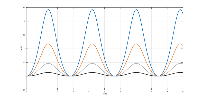
Figure 1: Time evolution of $\|\varphi_{k}(t)\|$ governed by the Davies–Swanson oscillator with initial data defined by $\l_{0}=(1,-\mathrm{i})$. The color coding is black for $k=0$, grey for $k=1$, orange for $k=2$ and blue for $k=3$. The parameters of the oscillator are chosen as $\omega_{0}=1$ and $\delta=0.5$ such that the solution $\varphi_{k}(t)$ exists for all $t\in\mathds{R}$. In all four cases the norms considerably depart from unity, the larger $k$ is, the stronger they deviate.

5.3 Evolution of the roots for the diffusion equation

Our proceeding for the one-dimensional diffusion equation is analogue to the Davies–Swanson oscillator,

$$H_{D}=-2\mathrm{i}\alpha\begin{pmatrix}1&0\\  0&0\end{pmatrix},\qquad\alpha\in\mathds{C}\,.$$

Since $(\Omega H_{D})^{2}=0$ we find for the Hamiltonian system $\dot{S}_{t}=\Omega H_{D}S_{t}$ with $S_{0}=\mathrm{Id}_{2}$ that

$$S_{t}=\exp(t\Omega H_{D})=\mathrm{Id}_{2}+t\,\Omega H_{D}=\begin{pmatrix}1&0\\ -2\mathrm{i}\alpha t&1\end{pmatrix}\ .$$

for all times $t\in\mathds{R}$. Since the spectrum of $\operatorname{Im}(H_{D})$ is $\sigma=\{-2\operatorname{Re}(\alpha),0\}$ an initial positive Lagrangian subspace stays positive for all $t\geq 0$ if $\operatorname{Re}(\alpha)\geq 0$. In practice $\operatorname{Re}(\alpha)$ measures the directed transfer rate of the medium, i.e. the larger $\operatorname{Re}(\alpha)$ the more transmissible our system is. If $\operatorname{Re}(\alpha)\geq 0$ we study the standard setting where particles are transferred from regions with higher concentration to regions with lower concentration. However, to provide a full theoretical description we investigate also the case $\operatorname{Re}(\alpha)<0$ in the following result.

Lemma 5.3 (Positive Lagrangian subspace).

Let $L_{0}=\operatorname{span}\{l_{0}\}$ be a positive Lagrangian subspace spanned by a normalised Lagrangian frame $l_{0}=(p_{0},q_{0})\in\mathds{C}\oplus\mathds{C}$. Then, $L_{t}=S_{t}L_{0}$ is positive for all $t\in\mathds{R}$ if $\operatorname{Re}(\alpha)\geq 0$ and for $t\in[0,T[$ with

$$T:=\left(-2\operatorname{Re}(\alpha)|p_{0}|^{2}\right)^{-1}$$

if $\operatorname{Re}(\alpha)<0$.

Proof.

A direct calculation yields

$$S^{*}_{t}\Omega S_{t}=\begin{pmatrix}1&2\mathrm{i}\bar{\alpha}t\\ 0&1\end{pmatrix}\begin{pmatrix}2\mathrm{i}\alpha t&-1\\ 1&0\end{pmatrix}=\begin{pmatrix}4\mathrm{i}\operatorname{Re}(\alpha)t&-1\\ 1&0\end{pmatrix}$$

and thus

$$n^{-2}_{t}=h(S_{t}l_{0},S_{t}l_{0})=\frac{1}{2i}\begin{pmatrix}\bar{p}_{0}&\bar{q}_{0}\end{pmatrix}\begin{pmatrix}4\mathrm{i}\operatorname{Re}(\alpha)t&-1\\ 1&0\end{pmatrix}\begin{pmatrix}p_{0}\\ q_{0}\end{pmatrix}=1+2\operatorname{Re}(\alpha)|p_{0}|^{2}t$$

where we used that the normalisation of $l_{0}$ implies $\operatorname{Im}(p_{0}\bar{q}_{0})=1$. ∎

In the following we only consider times $t$ such that $L_{t}$ is a positive Lagrangian subspace. The calculation of the normalisation in the previous proof gives

$$e^{\beta_{t}}=n^{1/2}_{t}=\left(1+2\operatorname{Re}(\alpha)|p_{0}|^{2}t\right)^{-1/4}.$$

It remains to determine the factors for the polynomial recursion,

$$m_{t}=n_{t}^{2}\,h(S_{t}l_{0},S_{t}\bar{l}_{0})=2n_{t}^{2}\operatorname{Re}(\alpha)\bar{p}_{0}^{2}t,\qquad\widetilde{m}_{t}=m_{t}+n^{2}_{t}q^{-1}_{t}\bar{q}_{t}=\frac{\bar{q}_{0}-2\mathrm{i}\alpha t\bar{p}_{0}}{q_{0}-2\mathrm{i}\alpha tp_{0}}\ .$$

As direct example we investigate the heat equation, $\alpha=1$, again with the special initial value $l_{0}=(1,-\mathrm{i})$. One can easily derive the explicit formulas

$$n^{-2}_{t}=1+2t,\qquad m_{t}=\frac{2t}{1+2t}\ .$$

Moreover, $\tilde{m}_{t}=\frac{2t-1}{2t+1}$ and the evolution of the roots of the second excited state $\varphi_{2}(t)$ is given by

$$x_{1/2}(t) =\pm\,n^{-1}_{t}q_{t}\sqrt{\tfrac{1}{2}\widetilde{m}_{t}}$$

$$=\pm\sqrt{\tfrac{1}{2}(1+2t)(1-2t)}\,.$$

Hence, the roots are propagated towards the origin and vanish at $t=0.5$. The behaviour for the roots of the third excited states follows similarly. Figures 2 below displays the evolution of the absolute value of the first three excited states $|\varphi_{k}(t)|$, $k=0,1,2,3$, in the described setting.

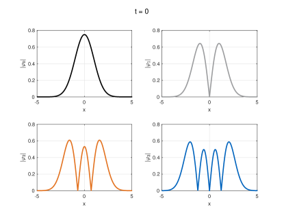
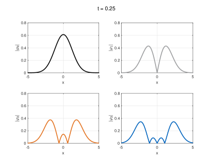
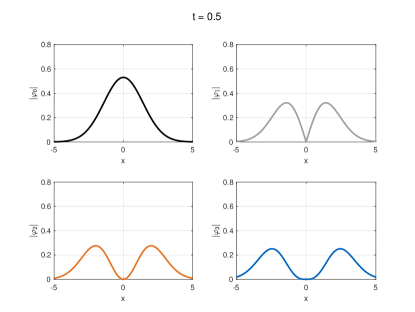
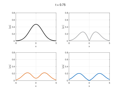
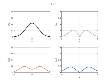
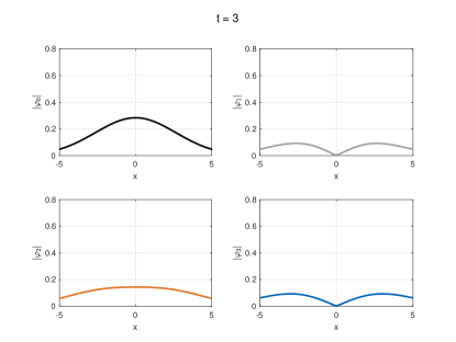
Figure 2: Time evolution of the state $|\varphi_{k}(t)|$ governed by the heat equation with initial data defined by $\l_{0}=(1,-\mathrm{i})$ at times $t=0$ (upper left), $t=0.25$ (upper right), $t=0.5$ (middle left), $t=0.75$ (middle right), $t=1$ (lower left) and $t=3$ (lower right). The color coding is black for $k=0$, grey for $k=1$, orange for $k=2$ and blue for $k=3$. We find the predicted behaviour, the roots of $\varphi_{2}$ and $\varphi_{3}$ are vanishing at $t=0.5$, the coherent state $\varphi_{0}$ is slowly damped due to the factor $e^{\beta_{t}}$.

5.4 Multivariate diffusion equation

Our findings for the diffusion equation can easily be generalised to several dimensions. Let

$$\partial_{t}\rho=\alpha\Delta\rho\quad\text{with}\quad H_{D}=-2\mathrm{i}\alpha\begin{pmatrix}\mathrm{Id}_{n}&0\\ 0&0\end{pmatrix}$$

and $\alpha\in\mathds{C}$. The flow emerges again as the matrix exponential

$$S_{t}=\exp(t\Omega H_{D})=\mathrm{Id}_{n}+t\,\Omega H_{D}=\begin{pmatrix}\mathrm{Id}_{n}&0\\ -2\mathrm{i}\alpha t\,\mathrm{Id}_{n}&\mathrm{Id}_{n}\end{pmatrix}$$

satisfying

$$S^{*}_{t}\Omega S_{t}=\begin{pmatrix}4\mathrm{i}\operatorname{Re}(\alpha)t\,\mathrm{Id}_{n}&-\mathrm{Id}_{n}\\ \mathrm{Id}_{n}&0\end{pmatrix}\ .$$

Hence, our statements of Lemma 5.3 on positive Lagrangian subspaces and the existence of the time evolution can immediately be lifted to several dimensions as follows:

Lemma 5.4 (Positive Lagrangian subspace).

Let $L_{0}=\operatorname{span}\{Z_{0}\}$ be a positive Lagrangian subspace spanned by a normalised Lagrangian frame $Z_{0}=(P_{0};Q_{0})\in\mathds{C}^{2n\times n}$. Then, the normalisation is given by

$$N^{-2}_{t}=\mathrm{Id}_{n}+2\operatorname{Re}(\alpha)t\,P^{*}_{0}P_{0}$$

and $L_{t}=S_{t}L_{0}$ is positive for all $t\in\mathds{R}$ if $\operatorname{Re}(\alpha)\geq 0$. Otherwise, denote by $\lambda_{\mathrm{max}}$ the eigenvalue of $P_{0}$ with the largest absolute value. Then, $L_{t}$ is positive for all $t\in[0,T[$ with $T=(-2\operatorname{Re}(\alpha)|\lambda_{\mathrm{max}}|^{2})^{-1}$.

For our futher investigations we consider two dimensions and choose as an anisotropic initial value

$$P_{0}=\tfrac{1}{2\sqrt{2}}\begin{pmatrix}-1+\mathrm{i}&1+\mathrm{i}\\ 1+\mathrm{i}&-1+\mathrm{i}\end{pmatrix},\quad Q_{0}=\tfrac{1}{\sqrt{2}}\begin{pmatrix}1+\mathrm{i}&1-\mathrm{i}\\ 1-\mathrm{i}&1+\mathrm{i}\end{pmatrix}\ .$$

The corresponding wavepacket $\varphi_{k}(Z_{0})$, $k\in\mathds{N}^{2}$ and $Z_{0}=(P_{0};Q_{0})$, is determined by the width matrix of the coherent state $P_{0}Q^{-1}_{0}=\tfrac{\mathrm{i}}{2}\mathrm{Id}_{2}$ and the recursion matrix of the polynomial prefactor

$$M_{0}=Q^{-1}_{0}\bar{Q}_{0}=\begin{pmatrix}0&1\\ 1&0\end{pmatrix}\ .$$

Since $M_{0}$ is not a diagonal matrix the wavepackets are not simple tensor products of one-dimensional Hermite functions, but can be expressed by means of the Laguerre polynomials, see Appendix  D. For the time evolution we can infer from $P^{*}_{0}P_{0}=\tfrac{1}{2}\mathrm{Id}_{2}$,

$$N_{t}=\left(\mathrm{Id}_{2}+2\operatorname{Re}(\alpha)t\,P^{*}_{0}P_{0}\right)^{-1/2}=(1+\operatorname{Re}(\alpha)t)^{-1/2}\,\mathrm{Id}_{2}\ ,$$

and $e^{\beta_{t}}=(\det N_{t})^{1/2}=(1+\operatorname{Re}(\alpha)t)^{-n/4}$. This information fully describes the propagated coherent state for $t\geq 0$ if $\operatorname{Re}(\alpha)\geq 0$ or $t\in[0;-\frac{1}{\operatorname{Re}(\alpha)}[$ otherwise.

For the evolution of the excited states we moreover need to determine the recursion matrix $\widetilde{M}_{t}$ defined in Corollary 4.6. We find

$$\widetilde{M}_{t}=N^{2}_{t}\left(-\operatorname{Re}(\alpha)t+\frac{1+\bar{\alpha}t}{1+\alpha t}\right)\,\begin{pmatrix}0&1\\ 1&0\end{pmatrix}\ ,$$

so that the circular structure of the wavepackets discussed in Appendix D is preserved.

Depending on the sign of the real part of $\alpha$ we can distinguish two different cases for the diffusion. Our results thereby agree with the basic mathematical theory of diffusion: the diffusion rate $\operatorname{Re}(\alpha)$ is proportional to the gradient of the concentration that is modelled. In more detail, diffusion occurs in the opposite direction of the increasing concentration, see [C75, §1.2]. Hence, $\operatorname{Re}(\alpha)>0$ corresponds to a diffusion to the outside and a spreading coherent state. In this case our model is well-defined for all times $t\geq 0$ and the norm is slowly decaying. We illustrate this case by means of the classical heat equation, $\alpha=1$. Then,

$$N_{t}=(1+t)^{-1/2}\,\mathrm{Id}_{2}\ ,\quad\widetilde{M}_{t}=\frac{1-t}{1+t}\begin{pmatrix}0&1\\ 1&0\end{pmatrix}\ ,$$

the wavepackets are damped. This behaviour is displayed in Figure 3.

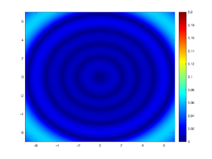
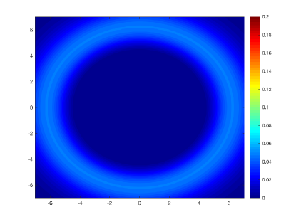
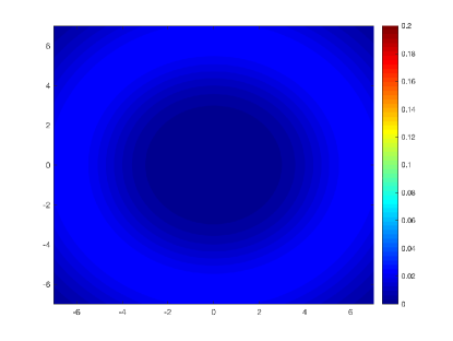
Figure 3: Time evolution of the state $|\varphi_{k}(t)|$ governed by the heat equation for $k=(4,6)$ at times $t=0$ (upper left), $t=0.25$ (upper right), $t=0.5$ (lower left) and $t=1.5$ (lower right). As $\operatorname{Re}(\alpha)>0$ the wavepacket is damped. Although the circular structure stays unaltered, real roots are vanishing due to the change of sign of the entries of $\widetilde{M}_{t}$.

On the other side $\operatorname{Re}(\alpha)<0$ models a diffusion to the origin. In our model the norm is increasing and the propagation collapses at $T=-\operatorname{Re}(\alpha)^{-1}$. We examine this case for $\alpha=-1+\tfrac{\mathrm{i}}{4}$. Then,

$$N_{t}=(1-t)^{-1/2}\,\mathrm{Id}_{2}\quad\text{and}\quad\widetilde{M}_{t}=\frac{1}{1-t}\left(t+\frac{1-t-\tfrac{\mathrm{i}}{4}t}{1-t+\tfrac{\mathrm{i}}{4}t}\right)\begin{pmatrix}0&1\\ 1&0\end{pmatrix}\ ,$$

what corresponds to an increasing norm of the wavepackets. By taking $\operatorname{Im}(\alpha)\neq 0$ we additionally include dynamics induced by the Schrödinger part of the equation. Consequentially, the wavepackets tend to the origin at the beginning, but are then broadened again. Figure 4 shows the propagation for this setting.

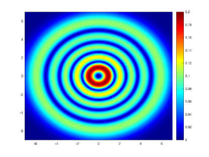
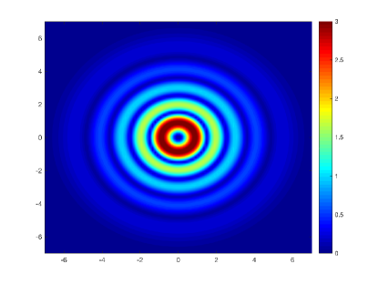
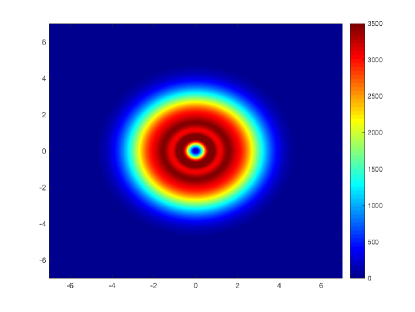
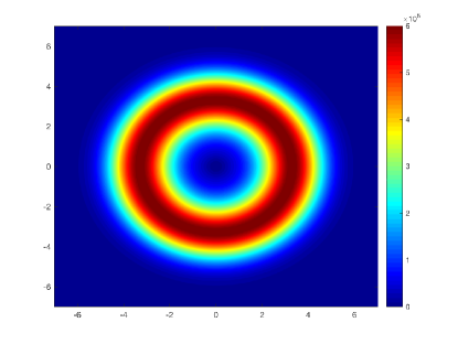
Figure 4: Time evolution of the state $|\varphi_{k}(t)|$, $k=(4,6)$, for $\alpha=-1+\tfrac{\mathrm{i}}{4}$ at times $t=0$ (upper left), $t=0.25$ (upper right), $t=0.75$ (lower left) and $t=0.9$ (lower right). The norm of the wavepackets is significantly increasing over time. The circles first tend to the origin as $\operatorname{Re}(\alpha)<0$, but then the imaginary part of $\alpha$ encounters and broadens the evolution.

Appendix A Weyl calculus

Let us recall a few standard results about products and Weyl quantisation, see [CR12, Chapter 2] for background. We consider smooth phase space functions $a,b$ so that

$$\operatorname{Op}[a]\psi(x)=(2\pi\varepsilon)^{-n}\int_{\mathds{R}^{2n}}a(\xi,\tfrac{1}{2}(x+y))\mathrm{e}^{\frac{\mathrm{i}}{\varepsilon}\xi\cdot(x-y)}\psi(y)d\xi dy$$

together with the compositions $\operatorname{Op}[a]\operatorname{Op}[b]$ and $\operatorname{Op}[b]\operatorname{Op}[a]$ are well-defined linear operators on dense subsets of $L^{2}(\mathds{R}^{n})$. The symbol of the operator product is the so-called Moyal product of $a$ and $b$,

$$\operatorname{Op}[a]\operatorname{Op}[b]=\operatorname{Op}[a\sharp b]\ .$$

If one of the two symbols $a$ or $b$ is a polynomial of degree $\leq 2$, then

$$a\sharp b=ab+\frac{\mathrm{i}\varepsilon}{2}\nabla a\cdot\Omega\nabla b-\frac{\varepsilon^{2}}{8}\operatorname{tr}\left(D^{2}a\Omega D^{2}b\Omega^{T}\right)\ ,$$

where $\nabla=\nabla_{p,q}$ and

$$\Omega=\begin{pmatrix}0&-\mathrm{Id}_{n}\\ \mathrm{Id}_{n}&0\end{pmatrix}\in\mathds{R}^{2n\times 2n}\ .$$

Consequently, the commutator can be written as

$$[\operatorname{Op}[a],\operatorname{Op}[b]]=\mathrm{i}\varepsilon\operatorname{Op}[\nabla a\cdot\Omega\nabla b]\ .$$ (A.1)

In particular, the canonical commutation relations can be quickly verified as

$$[\hat{q}_{j},\hat{p}_{k}]=\mathrm{i}\varepsilon\nabla q_{j}\cdot\Omega\nabla p_{k}=\mathrm{i}\varepsilon\begin{pmatrix}0\\ e_{j}\end{pmatrix}\cdot\begin{pmatrix}0\\ e_{k}\end{pmatrix}=\mathrm{i}\varepsilon\delta_{jk}\ .$$

Another application of the product rule yields that the Weyl quantisation of a symmetric quadratic form equals the quadratic form in $\hat{z}$.

Lemma A.1 (Quadratic symbol).

We consider

$$H=\begin{pmatrix}H_{pp}&H_{pq}\\ H_{qp}&H_{qq}\end{pmatrix}\in\mathds{C}^{2n\times 2n}\ .$$

Then, $\operatorname{Op}[z\cdot Hz]=\hat{z}\cdot H\hat{z}+\frac{\mathrm{i}\varepsilon}{2}\operatorname{tr}(H_{qp}-H_{pq})$. In particular,

$$\operatorname{Op}[z\cdot Hz]=\hat{z}\cdot H\hat{z}\ ,\quad\text{if}\quad H=H^{T}\ .$$

Proof.

We compute

$$\hat{z}\cdot H\hat{z}=\operatorname{Op}[z\cdot Hz]+\frac{\mathrm{i}\varepsilon}{2}\sum_{j,k=1}^{2n}\nabla z_{j}\cdot\Omega H_{jk}\nabla z_{k}=\operatorname{Op}[z\cdot Hz]+\frac{\mathrm{i}\varepsilon}{2}\operatorname{tr}(-H_{pq}+H_{qp})\ ,$$

since $\sum_{j,k=1}^{2n}H_{jk}(e_{j}\cdot\Omega e_{k})=-H_{1n}-\cdots-H_{n,2n}+H_{n1}+\cdots+H_{2n,n}=\operatorname{tr}(-H_{pq}+H_{qp})$  . ∎

Appendix B Dynamics of the metric and the complex structure

We provide a Lagrangian frame’s proof for Theorem 4.3, that states the Riccati equations for the symplectic metric and the complex structure of the positive Lagrangian $L_{t}=S_{t}L_{0}$, that is,

$$\dot{G}_{t} = \operatorname{Re}H_{t}\Omega G_{t}-G_{t}\Omega\operatorname{Re}H_{t}-\operatorname{Im}H_{t}-G_{t}\Omega\operatorname{Im}H_{t}\Omega G\ ,$$

$$\dot{J}_{t} = \Omega\operatorname{Re}H_{t}J_{t}-J_{t}\Omega\operatorname{Re}H_{t}+\Omega\operatorname{Im}H_{t}+J_{t}\Omega\operatorname{Im}H_{t}J_{t}\ .$$

Proof.

We only work for $J_{t}$, since $G_{t}=\Omega J_{t}$. Let $Z_{0}\in F_{\rm n}(L_{0})$ and consider an invertible matrix $N_{t}\in\mathds{C}^{n\times n}$ so that $Z_{t}=S_{t}Z_{0}N_{t}\in F_{\rm n}(L_{t})$. We then have $J_{t}=-\operatorname{Re}(Z_{t}Z_{t}^{*})\Omega$. As in the proof of Propositon 4.2 we obtain

$$0 = \partial_{t}N_{t}^{*}N_{t}^{-*}+\tfrac{\mathrm{i}}{2}N_{t}(S_{t}Z_{0})^{*}(H_{t}-\bar{H}_{t})(S_{t}Z_{0})N_{t}+N_{t}^{-1}\partial_{t}N_{t}$$

$$= \partial_{t}N_{t}^{*}N_{t}^{-*}-Z_{t}^{*}\operatorname{Im}H_{t}Z_{t}+N_{t}^{-1}\partial_{t}N_{t}\ .$$

Next we differentiate $Z_{t}$ so that

$$\dot{Z}_{t}=\Omega H_{t}S_{t}Z_{0}N_{t}+S_{t}Z_{0}\partial_{t}N_{t}=\Omega H_{t}Z_{t}+Z_{t}N_{t}^{-1}\partial_{t}N_{t}\ .$$

Therefore,

$$\partial_{t}(Z_{t}Z_{t}^{*}) = \Omega H_{t}Z_{t}Z_{t}^{*}+Z_{t}N_{t}^{-1}\partial_{t}N_{t}Z_{t}^{*}+Z_{t}Z_{t}^{*}\bar{H}_{t}\Omega^{T}+Z_{t}\partial_{t}N_{t}^{*}N_{t}^{-*}Z_{t}^{*}$$

$$= \Omega H_{t}Z_{t}Z_{t}^{*}+Z_{t}Z_{t}^{*}\bar{H}_{t}\Omega^{T}+Z_{t}Z_{t}^{*}\operatorname{Im}H_{t}Z_{t}Z_{t}^{*}\ .$$

Since $\operatorname{Im}(Z_{t}Z_{t}^{*})=-\Omega$, we then have

$$\partial_{t}\operatorname{Re}(Z_{t}Z_{t}^{*}) = \Omega\operatorname{Re}H_{t}\operatorname{Re}(Z_{t}Z_{t}^{*})+\Omega\operatorname{Im}H_{t}\Omega-\operatorname{Re}(Z_{t}Z_{t}^{*})\operatorname{Re}H_{t}\Omega$$

$$+\operatorname{Re}(Z_{t}Z_{t}^{*})\operatorname{Im}H_{t}\operatorname{Re}(Z_{t}Z_{t}^{*})$$

and the claimed equation $\dot{J}_{t}=\Omega\operatorname{Re}H_{t}J_{t}+\Omega\operatorname{Im}H_{t}-J_{t}\Omega\operatorname{Re}H_{t}+J_{t}\Omega\operatorname{Im}H_{t}J_{t}\ .$ ∎

Appendix C Multivariate polynomials

Analysing Hagedorn wave packets and their dynamics, we have encountered multivariate polynomials generated by the following type of recursion relation.

Definition C.1 (Polynomial recursion).

Let $M\in\mathds{C}^{n\times n}$ be symmetric and $c\in\mathds{C}$. We define a set of multivariate polynomials $p_{\alpha}(x)$ by the recursion relation

$$p_{0}(x)=c\ ,\qquad\left(p_{\alpha+e_{j}}(x)\right)^{n}_{j=1}=xp_{\alpha}(x)-M\nabla p_{\alpha}(x)$$ (C.1)

with $x\in\mathds{C}^{n}$ and $\alpha\in\mathds{N}_{0}^{n}$.

Together with $c=1$ the matrix $M=0$ generates the monomials $p_{\alpha}(x)=x^{\alpha}$, while the identity matrix $M=\mathrm{Id}$ determines tensor products of simple Hermite polynomials.
If $Q\in\mathds{C}^{n\times n}$ is the lower block of a normalised Lagrangian frame

$$Z=\begin{pmatrix}P\\ Q\end{pmatrix}\in\mathds{C}^{2n\times n}\ ,$$

then the matrix $M=Q^{-1}\bar{Q}$ generates the polynomial prefactor $p^{M}_{\alpha}$ of the Hagedorn wave packets, that is,

$$\varphi_{\alpha}(Z;x)=\tfrac{1}{\sqrt{\alpha!}}p^{M}_{\alpha}\left(\sqrt{\tfrac{2}{\varepsilon}}\,Q^{-1}x\right)\,\varphi_{0}(Z;x)\ ,\qquad\alpha\in\mathds{N}^{n}\ .$$ (C.2)

Lemma C.2 (Properties of the recursion matrix).

Let $Z=(P;Q)\in\mathds{C}^{2n\times n}$ be a normalised Lagrangian frame. Then, $M=Q^{-1}\bar{Q}$ is unitary and symmetric.

Proof.

As argued in Corollary 4.6 the symmetry of $M$ follows since $QQ^{*}=\left(\operatorname{Im}(PQ^{-1})\right)^{-1}$ is real symmetric,

$$M-M^{T}=Q^{-1}\bar{Q}-Q^{*}Q^{-T}=Q^{-1}\left(\bar{Q}Q^{T}-QQ^{*}\right)Q^{-T}=0\,.$$

The unitarity is a direct consequence,

$$MM^{*}=M\bar{M}=Q^{-1}\bar{Q}\bar{Q}^{-1}Q=\mathrm{Id}_{n}\,.$$

∎

All the polynomials sequences of Definition C.1 are multivariate versions of orthogonal polynomials determined by Favard’s theorem. In the univariate setting, a polynomial sequence $p_{n}(x)$, $n\in\mathds{N}_{0}$, is called an Appell sequences, if $p_{n}^{\prime}(x)=np_{n-1}(x)$ for all $n\geq 1$. The Hermite polynomials are prominent examples and the only orthogonal Appell sequence. In several dimensions this property generalises to the following gradient formula, which is due to [DKT15, Lemma 6].

Lemma C.3 (Gradient formula).

Let $M\in\mathds{C}^{n\times n}$ be symmetric and $c\in\mathds{C}$. The polynomials defined by the recursion relation (C.1) satisfy

$$\nabla_{x}p_{\alpha}(x)=\left(\alpha_{j}p_{\alpha-e_{j}}(x)\right)^{n}_{j=1}$$

for all $\alpha\in\mathds{N}_{0}^{n}$ and $x\in\mathds{C}^{n}$.

Proof.

We argue by induction and assume that the gradient formula holds for a fixed $\alpha\in\mathds{N}_{0}^{n}$. Differentiating the recursion relation, we get

$$\partial_{k}p_{\alpha+e_{j}} = \delta_{kj}p_{\alpha}+x_{j}\partial_{k}p_{\alpha}-e_{j}\cdot M\nabla\partial_{k}p_{\alpha}=\delta_{kj}p_{\alpha}+\alpha_{k}(x_{j}p_{\alpha-e_{k}}-e_{j}\cdot M\nabla p_{\alpha-e_{k}})$$

$$= \delta_{kj}p_{\alpha}+\alpha_{k}p_{\alpha+e_{j}-e_{k}}=(\alpha+e_{j})_{k}p_{\alpha+e_{j}-e_{k}}\ .$$

∎

Appendix D Wavepackets in one and two dimensions

The examples in Section 5 focus on Hagedorn wavepackets in one or two dimensions. To explain the varying forms we encounter we briefly discuss their roots. Let $Z=(P;Q)\in\mathds{C}^{2n\times n}$ be a normalised Lagrangian frame and $M=Q^{-1}\bar{Q}$. The corresponding wavepackets then emerge as (C.2). Hence, the roots of the wavepackets can be directly deduced from the roots of the polynomial $p^{M}_{\alpha}$.

D.1 One dimension

For a positive Lagrangian subspace $L=\operatorname{span}\{l\}$, $l\in\mathds{C}\oplus\mathds{C}$, the corresponding states are simply rescaled Hermite functions, i.e. with $l=(p,q)$ we find for all $\alpha\in\mathds{N}$

$$\varphi_{\alpha}(l;x)=\tfrac{m^{\alpha/2}}{\sqrt{\alpha!}}\,h_{\alpha}(\tfrac{2}{\sqrt{\varepsilon}}\tfrac{x}{q\sqrt{m}})\,\varphi_{0}(l;x)\,$$

where $m=q^{-1}\bar{q}\in\mathds{C}$ and $h_{k}$ denotes the $\alpha$-th probabilistic Hermite polynomial defined by

$$h_{-1}(x)=0,\qquad h_{0}(x)=1,\qquad h_{\alpha+1}(x)=xh_{\alpha}(x)-\alpha h_{\alpha-1}(x)\quad\forall\alpha\geq 0\,.$$

The roots of the wavepacket therefore depend on $q\sqrt{m}=q\left(\frac{\bar{q}}{q}\right)^{1/2}$. If this value is real, the wavepacket shows $\alpha$ distinct roots, otherwise the roots vanish, see Section 5.3.

D.2 Two dimensions

In two dimensions, the wavepackets relate to the Hermite functions only in special cases. The following result is a special case of [DKT15, Corollary 9]. We provide a proof here for a self-contained reading.

Lemma D.1.

Let

$$M=\begin{pmatrix}m_{1}&m_{3}\\ m_{3}&m_{2}\end{pmatrix}\in\mathds{C}^{2\times 2}\,.$$

and consider polynomials $(p^{M}_{\alpha})_{\alpha\in\mathds{N}^{2}}$ generated by $M$ via the recursion relation $p^{M}_{\alpha}(x)=0$ if $\alpha\notin\mathds{N}^{2}$,

$$p_{0}^{M}(x)=1,\qquad\begin{pmatrix}p_{(\alpha_{1}+1,\alpha_{2})}\\ p_{(\alpha_{1},\alpha_{2}+1)}\end{pmatrix}(x)=xp_{\alpha}(x)-M\begin{pmatrix}\alpha_{1}p_{(\alpha_{1}-1,\alpha_{2})}\\ \alpha_{2}p_{(\alpha_{1},\alpha_{2}-1)}\end{pmatrix}(x)\quad\forall x\in\mathds{R}^{2}\,.$$

If $m_{3}=0$ the polynomials $(p^{M}_{\alpha})_{\alpha\in\mathds{N}^{2}}$ can be written as

$$p^{M}_{\alpha}(x)=m^{\alpha_{1}/2}_{1}m^{\alpha_{2}/2}_{2}\,h_{\alpha_{1}}\left(\tfrac{x_{1}}{\sqrt{m_{1}}}\right)h_{\alpha_{2}}\left(\tfrac{x_{2}}{\sqrt{m_{2}}}\right)\,.$$

If $m_{1}=m_{2}=0$ the polynomials appear as

$$p^{M}_{\alpha}(x)=\begin{cases}(-m_{3})^{\alpha_{2}}\alpha_{2}!x_{1}^{\alpha_{1}-\alpha_{2}}L^{(\alpha_{1}-\alpha_{2})}_{\alpha_{2}}\left(\frac{x_{1}x_{2}}{m_{3}}\right)&\text{if}\ \alpha_{1}\geq\alpha_{2}\\ (-m_{3})^{\alpha_{1}}\alpha_{1}!x_{2}^{\alpha_{2}-\alpha_{1}}L^{(\alpha_{2}-\alpha_{1})}_{\alpha_{1}}\left(\frac{x_{1}x_{2}}{m_{3}}\right)&\text{if}\ \alpha_{1}<\alpha_{2}\end{cases}\ ,$$

where $L^{(\gamma)}_{\ell}$ denotes the $\ell$-th associated or generalised Laguerre polynomial.

Proof.

Both cases follow by induction. For $m_{3}=0$, we have

$$p_{(\alpha_{1}+1,\alpha_{2})}(x) =x_{1}p_{(\alpha_{1},\alpha_{2})}(x)-m_{1}\alpha_{1}p_{(\alpha_{1}-1,\alpha_{2})}(x)$$

$$=m^{\alpha_{2}/2}_{2}h_{\alpha_{2}}\left(\tfrac{x_{2}}{\sqrt{m_{2}}}\right)\left(m^{\alpha_{1}/2}_{1}x_{1}h_{\alpha_{1}}\left(\tfrac{x_{1}}{\sqrt{m_{1}}}\right)-m^{(\alpha_{1}+1)/2}_{1}\alpha_{1}h_{\alpha_{1}-1}\left(\tfrac{x_{1}}{\sqrt{m_{1}}}\right)\right)$$

$$=m^{(\alpha_{1}+1)/2}_{1}m^{\alpha_{2}/2}_{2}h_{\alpha_{2}}\left(\tfrac{x_{2}}{\sqrt{m_{2}}}\right)\left(\tfrac{x_{1}}{\sqrt{m_{1}}}h_{\alpha_{1}}\left(\tfrac{x_{1}}{\sqrt{m_{1}}}\right)-\alpha_{1}h_{\alpha_{1}-1}\left(\tfrac{x_{1}}{\sqrt{m_{1}}}\right)\right)$$

$$=m^{(\alpha_{1}+1)/2}_{1}m^{\alpha_{2}/2}_{2}h_{\alpha_{1}+1}\left(\tfrac{x_{1}}{\sqrt{m_{1}}}\right)h_{\alpha_{2}}\left(\tfrac{x_{2}}{\sqrt{m_{2}}}\right)\,.$$

The claim for $p_{(\alpha_{1},\alpha_{2}+1)}$ can be proven similarly. For the generalised Laguerre polynomials we can use

$$L^{(\gamma)}_{\ell}=L^{(\gamma+1)}_{\ell}-L^{(\gamma+1)}_{\ell-1}$$

for all $\gamma,\ell\in\mathds{N}$. Then we find for $m_{1}=m_{2}=0$ if $\alpha_{1}\geq\alpha_{2}$,

$$p_{(\alpha_{1}+1,\alpha_{2})}(x) =x_{1}p_{(\alpha_{1},\alpha_{2})}(x)-m_{3}\alpha_{2}p_{(\alpha_{1},\alpha_{2}-1)}(x)$$

$$=(-m_{3})^{\alpha_{2}}\alpha_{2}!x_{1}^{\alpha_{1}+1-\alpha_{2}}\left(L^{(\alpha_{1}-\alpha_{2})}_{\alpha_{2}}\left(\tfrac{x_{1}x_{2}}{m_{3}}\right)+L^{(\alpha_{1}-\alpha_{2}+1)}_{\alpha_{2}-1}\left(\tfrac{x_{1}x_{2}}{m_{3}}\right)\right)$$

$$=(-m_{3})^{\alpha_{2}}\alpha_{2}!x_{1}^{\alpha_{1}+1-\alpha_{2}}L^{(\alpha_{1}+1-\alpha_{2})}_{\alpha_{2}}\left(\tfrac{x_{1}x_{2}}{m_{3}}\right)$$

and

$$p_{(\alpha_{1},\alpha_{2}+1)}(x) =x_{2}p_{(\alpha_{1},\alpha_{2})}(x)-m_{3}k_{1}p_{(\alpha_{1}-1,\alpha_{2})}(x)$$

$$=(-m_{3})^{\alpha_{2}+1}\alpha_{2}!x_{1}^{\alpha_{1}-\alpha_{2}-1}\left(-\tfrac{x_{1}x_{2}}{m_{3}}L^{(\alpha_{1}-\alpha_{2})}_{\alpha_{2}}\left(\tfrac{x_{1}x_{2}}{m_{3}}\right)+\alpha_{1}L^{(\alpha_{1}-\alpha_{2}-1)}_{\alpha_{2}}\left(\frac{x_{1}x_{2}}{m_{3}}\right)\right)\,.$$

With

$$(\ell+1)L^{(\gamma)}_{\ell+1}(y) =(2\ell+1+\gamma-x)L^{(\gamma)}_{\ell}(y)-(\ell+\gamma)L^{(\gamma)}_{\ell-1}(y)\,,$$

$$\ell L^{(\gamma)}_{\ell}(y) =(\ell+\gamma)L^{(\gamma)}_{\ell-1}(y)-yL^{(\gamma+1)}_{\ell-1}(y)$$

it moreover holds

$$(\alpha_{2}+1)L^{(\alpha_{1}-\alpha_{2}-1)}_{\alpha_{2}+1}(y) =(\alpha_{2}+\alpha_{1}-y)L^{(\alpha_{1}-\alpha_{2}-1)}_{\alpha_{2}}(y)-(\alpha_{1}-1)L^{(\alpha_{1}-k_{2}-1)}_{\alpha_{2}-1}(y)$$

$$=\alpha_{1}L^{(\alpha_{1}-\alpha_{2}-1)}_{\alpha_{2}}(y)-y(L^{(\alpha_{1}-\alpha_{2}-1)}_{\alpha_{2}}+L^{(\alpha_{1}-\alpha_{2})}_{\alpha_{2}-1})$$

$$=-yL^{(\alpha_{1}-\alpha_{2})}_{\alpha_{2}}(y)+\alpha_{1}L^{(\alpha_{1}-\alpha_{2}-1)}_{\alpha_{2}}(y)\,.$$

Inserting $y=\tfrac{x_{1}x_{2}}{m_{3}}$ finishes the proof. ∎

Let

$$Q=\begin{pmatrix}q_{11}&q_{12}\\ q_{21}&q_{22}\end{pmatrix}\in\mathds{C}^{2\times 2}\,.$$

If $m_{3}=0$, the factorisation $M=Q^{-1}\bar{Q}$ implies $m_{1}=\bar{m}_{2}$ with $|m_{1}|=1$ and the Hagedorn wavepacket $\varphi_{\alpha}(Z)$ possesses at most $|\alpha|$-many real roots given by

$$q_{22}x_{1}-q_{12}x_{2} =c_{1}\eta_{1,j}\,,\qquad j=1,\ldots,\alpha_{1}\,,$$

$$-q_{21}x_{1}+q_{11}x_{2} =c_{2}\eta_{2,j}\,,\qquad j=1,\ldots,\alpha_{2}\,,$$

where $\eta_{i,j}$ denotes the $j$-th root of $h_{\alpha_{i}}$ and $c_{i}=\sqrt{\varepsilon m_{i}}\det(Q)$, $i=1,2$. Consequently, the roots form a lattice.

A matrix $Q$ that produces $m_{1}=m_{2}=0$ is of the form $q_{12}=\bar{m}_{3}q_{11}$, $q_{22}=\bar{m}_{3}q_{21}$. The unitarity of $M$ again yields $|m_{3}|=1$. The roots of $\varphi_{\alpha}(Z)$ therefore satisfy for $\alpha_{1}\geq\alpha_{2}$

$$(\bar{q}_{21}x_{1}-\bar{q}_{11}x_{2})^{j}=0\,,\qquad j=1,\ldots,\alpha_{1}-\alpha_{2}\,,$$

and

$$(\bar{q}_{21}x_{1}-\bar{q}_{11}x_{2})(q_{21}x_{1}-q_{11}x_{2}) =c_{3}\theta_{j},\,,\qquad j=1,\ldots,\alpha_{2}\,,$$

$$|q_{21}|^{2}x_{1}-|q_{11}|^{2}x_{2}-2\operatorname{Re}(q_{11}\bar{q}_{12})x_{1}x_{2} =c_{3}\theta_{j},\,,\qquad j=1,\ldots,\alpha_{2}\,,$$

where $\theta_{j}$, $j=1,\ldots,\alpha_{2}$ denotes the $j$-th root of the generalised Laguerre polynomial $L^{(\alpha_{1}-\alpha_{2})}_{\alpha_{2}}$ and $c_{3}=4\varepsilon\operatorname{Im}(q_{11}\bar{q}_{12})$. So, the roots of the wavepackets consist of at most $\alpha_{1}-\alpha_{2}$-many lines through the origin and $\alpha_{2}$-many ellipses whose distances are proportional to the roots of $L^{(\alpha_{1}-\alpha_{2})}_{\alpha_{2}}$, see Figure 3 and 4.

References

- [AV15] A. Aleman and J. Viola, Singular-value decomposition of solution operators to model evolution equations, Int. Math. Res. Not. IMRN (2015), no. 17, 8275–8288.
- [BMR13] A. M. Bloch, P. J. Morrison, and T. S. Ratiu, Gradient flows in the normal and Kähler metrics and triple bracket generated metriplectic systems, Recent trends in dynamical systems, Springer Proc. Math. Stat., vol. 35, Springer, Basel, 2013, 371–415.
- [C75] J. Crank, The mathematics of diffusion, Clarendon Press, Oxford, 1975.
- [CGHS12] E. Caliceti, S. Graffi, M. Hitrik, J. Sjösstrand, Quadratic PT-symmetric operators with real spectrum and similarity to self-adjoint operators, J. Phys. A, 45 (2012) 444007, 20 pp.
- [CR12] M. Combescure and D. Robert, Coherent states and applications in mathematical physics, Theoretical and Mathematical Physics, Springer, Dordrecht, 2012.
- [Dav99a] E. B. Davies, Pseudo-spectra, the harmonic oscillator and complex resonances, R. Soc. Lond. Proc. Ser. A Math. Phys. Eng. Sci. 455 (1999), no. 1982, 585–599.
- [Dav99b] E. B. Davies, Semi-classical states for non-self-adjoint Schrödinger operators, Comm. Math. Phys. 200 (1999).
- [DK04] E. B. Davies and A. B. J. Kuijlaars, Spectral asymptotics of the non-self-adjoint harmonic oscillator, J. London Math. Soc. (2) 70 (2004), no. 2, 420–426.
- [DKT15] H. Dietert, J. Keller, and S. Troppmann, An invariant class of wave packets for the Wigner transform, J. Math. Anal. Appl. 450 (2017), no. 2, 1317–1332.
- [GGN09] I. Gallagher, T, Gallay, F. Nier, Spectral Asymptotics for Large Skew-Symmetric Perturbations of the Harmonic Oscillator, Int. Math. Res. Not. IMRN (2009), no. 12, 2147–-2199.
- [GH14] V. Gradinaru and G. A. Hagedorn, Convergence of a semiclassical wavepacket based time-splitting for the Schrödinger equation, Numer. Math. 126 (2014), no. 1, 53–73.
- [GKRS14] E.-M. Graefe, H. J. Korsch, A. Rush, and R. Schubert, Classical and quantum dynamics in the (non-Hermitian) Swanson oscillator, J. Phys. A 48 (2015), no. 5, 055301, 16 pp.
- [GS11] E.-M. Graefe and R. Schubert, Wave-packet evolution in non-Hermitian quantum systems, Phys. Rev. A 83 (2011).
- [GS12] E.-M. Graefe and R. Schubert, Complexified coherent states and quantum evolution with non-Hermitian Hamiltonians, J. Phys. A 45 (2012), no. 24, 244033, 15 pp.
- [Hag80] G. A. Hagedorn, Semiclassical quantum mechanics. I. The limit for coherent states, Comm. Math. Phys. 71 (1980), no. 1, 77–93.
- [Hag85] G. A. Hagedorn, Semiclassical quantum mechanics. IV. Large order asymptotics and more general states in more than one dimension, Ann. Inst. H. Poincaré Phys. Théor. 42 (1985), no. 4, 363–374.
- [Hag98] G. A. Hagedorn, Raising and lowering operators for semiclassical wave packets, Ann. Physics 269 (1998), no. 1, 77–104.
- [Hel75] E. J. Heller, Time dependent approach to semiclassical dynamics, J. Chem. Phys. 62 (1975), no. 4, 1544–55.
- [Hel76] E. J. Heller, Time dependent variational approach to semiclassical dynamics, J. Chem. Phys. 64 (1976), no. 1, 63–73.
- [Hen14] R. Henry, Spectral instability for even non-selfadjoint anharmonic oscillators, J. Spectr. Theory 4 (2014).
- [Hep74] K. Hepp, The classical limit for quantum mechanical correlation functions, Comm. Math. Phys. 35 (1974), 265–277.
- [HP13] M. Hitrik and K. Pravda-Starov, Eigenvalues and subelliptic estimates for non-selfadjoint semiclassical operators with double characteristics, Ann. Inst. Fourier 63 (2013), no. 3, 985–1032.
- [HSV13] M. Hitrik, J. Sjöstrand, and J. Viola, Resolvent estimates for elliptic quadratic differential operators, Anal. PDE 6 (2013), no. 1, 181–196.
- [Hör94] L. Hörmander, The Analysis of Linear Partial Differential Operators III, Grundlehren der Mathematischen Wissenschaften, Springer, Berlin, Heidelberg, 1994.
- [Hör95] L. Hörmander, Symplectic classification of quadratic forms, and general Mehler formulas, Math. Z. 219 (1995), no. 3, 413–449.
- [KSTV15] D. Krejcirik, P. Siegl, M. Tater, and J. Viola, Pseudospectra in non-Hermitian quantum mechanics, J. Math. Phys. 65 (2015), 103513.
- [Lit86] R. G. Littlejohn, The semiclassical evolution of wave packets, Phys. Rep. 138 (1986), no. 4-5, 193–291.
- [LRT13] H. Liu, O. Runborg, and N. M. Tanushev, Error estimates for Gaussian beam superpositions, Math. Comp. 82 (2013), no. 282, 919–952.
- [Lub08] C. Lubich, From quantum to classical molecular dynamics: reduced models and numerical analysis, Zurich Lectures in Advanced Mathematics, European Mathematical Society (EMS), Zürich, 2008.
- [Moi11] N. Moiseyev, Non-Hermitian quantum mechanics, Cambridge University Press, Cambridge, 2011.
- [MR99] J. E. Marsden and T. S. Ratiu, Introduction to mechanics and symmetry, second ed., Texts in Applied Mathematics, vol. 17, Springer-Verlag, New York, 1999.
- [MS98] D. McDuff and D. Salamon, Introduction to symplectic topology, second ed., Oxford Mathematical Monographs, The Clarendon Press, Oxford University Press, New York, 1998.
- [Paz83] A. Pazy, Semigroups of linear operators and applications to partial differential equations, Springer-Verlag, New York, 1983.
- [Pra08] K. Pravda-Starov, Contraction semigroups of elliptic quadratic differential operators, Math. Z. 259 (2008), 363–391.
- [Sjö74] J. Sjöstrand, Parametrices for pseudodifferential operators with multiple characteristics, Ark. Mat. 12 (1974), 85–130.
- [Swa04] M. S. Swanson, Transition elements for a non-Hermitian quadratic Hamiltonian, J. Math. Phys. 45 (2004), no. 2, 585–601.
- [TE05] L. N. Trefethen and M. Embree, Spectra and pseudospectra, Princeton University Press, Princeton, NJ, 2005.
- [Vio16] J. Viola, The norm of the non-self-adjoint harmonic oscillator semigroup, Integral Equations Operator Theory 85 (2016), no. 4, 513–538
- [YU00] J.A. Yeazell and T. Uzer, The physics and chemistry of wave packets, Wiley, New York, 2000.