Classical lattice spin models involving singular interactions isotropic in spin space

Abstract

We address here a few classical lattice–spin models, involving $n-$component unit vectors ($n=2,3$), associated with a $D-$dimensional lattice $\mathbb{Z}^{D},~{}D=1,2$, and interacting via a pair potential restricted to nearest neighbours and being isotropic in spin space, i.e. defined by a function of the scalar product between the interacting spins. When the potential involves a continuous function of the scalar product, the Mermin–Wagner theorem and its generalizations exclude orientational order at all finite temperatures in the thermodynamic limit, and exclude phase transitions at finite temperatures when $D=1$; on the other hand, we have considered here some comparatively simple functions of the scalar product which are bounded from below, diverge to $+\infty$ for certain mutual orientations, and are continuous almost everywhere with integrable singularities. Exact solutions are presented for $D=1$, showing absence of phase transitions and absence of orientational order at all finite temperatures in the thermodynamic limit; for $D=2$, and in the absence of more stringent mathematical results, extensive simulations carried out on some of them point to the absence of orientational order at all finite temperatures, and suggest the existence of a Berezinskiǐ-Kosterlitz-Thouless transition.

I Introduction

The study of lattice spin models, both classical (on which we shall be concentrating here) and quantum, is an important chapter of Statistical Mechanics, where a number of mathematical results have been obtained, entailing absence or existence, and sometimes type, of phase transitions at finite temperatures, depending on lattice dimension, number of spin components, range and symmetry of the interaction.

The Mermin-Wagner theorem was first proven nearly 50 years ago in a quantum setting, for the isotropic spin Heisenberg model with finite–range exchange interactions Mermin and Wagner (1966a); *rMW001, and later extended by various Authors in a number of directions, e.g. to the classical setting, to other functions of the scalar product, or to longer–ranged interactions Mermin (1969); *rMW02; Thorpe (1971); Nenciu (1971); Vuillermot and Romerio (1975); see also a subsequent Review in Ref. Gelfert and Nolting (2001).

In the classical case, the Mermin–Wagner theorem and its generalizations Sinaǐ (1982); Georgii (1988); Ioffe et al. (2002); Gagnebin and Velenik (2014) hold for lattice–spin models, consisting of $n-$component unit vectors ($n\geq 2$), associated with a $D-$dimensional lattice $\Lambda_{D}$ ($D=1,2$ and typically $\Lambda_{D}=\mathbb{Z}^{D}$), and interacting via pair potentials which are isotropic in spin space, and usually translationally invariant (on the other hand, mathematical results have also been obtained which do not need any translational invariance Pfister (1981); Fröhlich and Pfister (1981); Picco (1983); *ntir04; van Enter and Fröhlich (1985); van Enter (1985); Fröhlich and Ueltschi (2015)); the distance dependence is usually taken to be suitably short-ranged. Their orientational dependences are defined by some functions of the scalar product between interacting spin pairs: the earlier mathematical results were obtained for rather smooth functions (simple polynomials), and conditions were later gradually relaxed, i.e. to the milder request of continuity, and, in some cases, even to less regular functions Ioffe et al. (2002); Gagnebin and Velenik (2014).

More explicitly, continuity is required in Refs. Ioffe et al. (2002); Gagnebin and Velenik (2014), and some singularities are also allowed for in Ref. Ioffe et al. (2002); we are restricting our present discussion to finite–range (actually, nearest–neighbour) interactions, and notice that mathematical results are known for long–range interactions as well (see, e.g., Refs. Georgii (1988); Ioffe et al. (2002); Gagnebin and Velenik (2014), and others quoted therein).

To fix notation and ideas, let $\mathbf{w}_{j}=(w_{j}^{1},w_{j}^{2},\cdots,w_{j}^{n})$ denotes the $n$–component unit vector (spin) associated with the $j-$th lattice site, with dimensionless coordinate vector $\mathbf{x}_{j}\in\mathbb{Z}^{D}$; two–component spins are parameterized by usual polar angles $\varphi_{j}$, and three–component spins are parameterized by usual spherical angles $\left(\theta_{j},~{}\phi_{j}\right)$. Here and in the following the interaction will be restricted to nearest neighbours and defined by

$$\Phi\equiv\Phi(\tau)=\epsilon F(\tau),~{}\tau\equiv\tau_{jk}=\mathbf{w}_{j}\cdot\mathbf{w}_{k},$$ (1)

where $\epsilon>0$ denotes a positive quantity setting energy and temperature scales (i.e. $T=k_{B}\mathcal{T}_{K}/\epsilon$, where $\mathcal{T}_{K}$ denotes the temperature in degrees Kelvin), and to be scaled away from the following formulae. For $2-$component spins, it will prove notationally convenient to define

$$\tau=\cos\Delta,\quad~{}\Delta\equiv\Delta_{jk}=\varphi_{j}-\varphi_{k}.$$ (2)

When $F(\tau)$ is a continuous function of its argument, the above theorems entail absence of orientational order in the thermodynamic limit at all finite temperatures Ioffe et al. (2002); when $D=n=2$, and under additional conditions, a Berezinskiǐ-Kosterlitz-Thouless (BKT), or, in more general terms, a BKT-like transition can be proven to exist Fröhlich and Spencer (1981); Minnhagen (1987); Pierson (1997); Gulácsi and Gulácsi (1998); Romano (2006); José (2013); van Enter and Shlosman (2002, 2005); the term “BKT-like” is used here to indicate a transition to a disordered low-temperature phase possessing slowly decaying correlations resulting in infinite susceptibility; in thermodynamic terms, the transition may be of infinite order (as in the more common, originally studied BKT case Fröhlich and Spencer (1981); Minnhagen (1987); Pierson (1997); Gulácsi and Gulácsi (1998); Romano (2006); José (2013); it was also later proven van Enter and Shlosman (2002, 2005) that it can turn first-order under certain conditions.

Cases where $F(\tau)$ possesses some singularity have been studied far less extensively (see also below). In fact one can envisage a multitude of singular interactions: models involving a finite number of jump discontinuities, as in sign or step models, are discussed in Appendix A; another family, also discussed there, involves constrained models, where whole regions of configuration space are excluded. We have chosen to start our investigation, so to speak, somewhere in between these two cases, from functional forms containing slowly divergent terms which do not disturb thermodynamics, i.e. from functional forms being bounded from below, continuous almost everywhere, slowly diverging to $+\infty$ for one (or a few) mutual orientations, and possessing integrable singularities. Thus the present paper addresses a few models whose functional forms are defined by

$$V(\tau) = -\ln(1+\tau),\quad n=2,$$ (3a)

$$W(\tau) = -\ln(1+\tau),\quad n=3,$$ (3b)

$$X(\tau) = -\ln(|\tau|),\quad n=3.$$ (3c)

In due course, comparisons will also be made with their extensively studied counterparts defined by

$$F(\tau) = -\tau,\quad\qquad~{}n=2,$$ (4a)

$$F(\tau) = -\tau,\quad\qquad n=3,$$ (4b)

$$F(\tau) = -P_{2}(\tau),\quad n=3,$$ (4c)

respectively, and simply referred to as “regular counterparts”.

Some models bearing similarities to ours [Eq. (3b)] have been investigated previously in the literature Niemeijer and Ruijgrok (1977); Ishimori (1982); Arovas et al. (1988); Parameswaran et al. (2009); Daniel and Manivannan (1998); *rsing6. More recent studies showed that such classical models are effective models obtained via mappings from quantum-mechanical treatments Ishimori (1982); Arovas et al. (1988); Parameswaran et al. (2009). The above singular models [Eqs. (3)], as well as some generalizations and linear combinations of them, can be solved exactly when $D=1$, allowing one to obtain thermodynamic and structural quantities in closed form; these are worked out in Appendix A, where other singular models, such as step or sign model and constrained ones are addressed as well. The three models in Eqs. (3) are studied by extensive Monte Carlo (MC) simulation for $D=2$ so as to explore the thermodynamic behavior of these models, on the one hand, and to unveil potential effects of the singularities in comparison with their regular counterparts, on the other hand.

The rest of the paper is organized as follows: in Sec. II we further discuss the singular models; our simulation methodology for $D=2$ is discussed in Section III along with with brief details on the finite-size approach we employ for the analysis of the simulation data. In Sec. IV we present the simulation results and finite-size scaling analysis used to extract the critical behavior for the models under consideration. We conclude the paper with Sec. V where we summarize our results.

II Remarks on the potential models

Both $V$ and $W$ attain their minimum at $\tau_{min}=1$, and slowly diverge to $+\infty$ as $\tau\rightarrow-1$; $X(\tau)$ attains its minima at $\tau_{min}=\pm 1$, and slowly diverges to $+\infty$ as $\tau\rightarrow 0$; the above functions are bounded from below, continuous almost everywhere, and possess integrable singularities; in these cases, an interaction diverging to $+\infty$ is still compatible with the thermodynamics and, by its very functional form, it can be expected to enforce some strengthening of short-range correlations. On the other hand, changing the sign in front of the “$\ln$” from “$-$” to “$+$” in (any of) Eqs. (3) would produce a rather dramatic effect, i.e. it would cause a divergence to $-\infty$ for some mutual orientations, and hence make the modified model not well defined at low temperatures Niemeijer and Ruijgrok (1977).

Series expansions of Eqs. (3) can be written down, i.e.

$$V(\tau) = \ln(2)+\lim_{q\rightarrow\infty}\mathcal{V}_{q},$$

$$\mathcal{V}_{q} = 2\sum_{l=1}^{q}\frac{(-1)^{l}}{l}\cos(l\Delta_{jk}),~{}0\leq\Delta_{jk}<\pi;$$ (5a)

$$W\tau) = \lim_{q\rightarrow\infty}\mathcal{W}_{q},$$

$$\mathcal{W}_{q} = \sum_{l=1}^{q}\frac{(-1)^{l}}{l}\tau^{l},~{}-1<\tau\leq 1;$$ (5b)

$$X(\tau) = \lim_{q\rightarrow\infty}\mathcal{X}_{q},$$

$$\mathcal{X}_{q} = \sum_{l=1}^{q}\frac{1}{l}(1-|\tau|)^{l},~{}0<|\tau|\leq 1;$$ (5c)

each $\mathcal{X}_{q}$ is a polynomial in $|\tau|$, where the coefficient in front of $|\tau|^{l}$ bears the sign $(-1)^{l}$; in other words sign alternation is a common feature of the three above expansions. Any of the above truncated expansions [Eqs. (5)] is a continuous function of $\tau$ which, by the Mermin-Wagner theorem and its generalizations Ioffe et al. (2002); Gagnebin and Velenik (2014), produces orientational disorder at all finite temperatures; let us now consider a generalization of $\mathcal{V}_{q}$, i.e.

$$\mathcal{F}_{q}=\sum_{l=1}^{q}c_{l}\cos(l\Delta),$$ (6)

where $c_{l}$ denote arbitrary real coefficients; the Mermin-Wagner theorem can be applied here as well; moreover, for a general ferromagnetic interaction (where all the coefficients $c_{l}$ are $\leq 0$), one can prove BKT behavior, based on its existence for Eq. (4a) Fröhlich and Spencer (1981) and on correlation inequalities, and also obtain a rigorous lower bound on the BKT transition temperature (see Ref. Romano (2006) and others quoted therein); unfortunately, the alternating signs in $\mathcal{V}_{q}$ prevent us from using this approach in general. Let us also mention in passing a simple specific case of Eq. (6), defined by

$$\mathcal{G}_{2}=c_{1}\cos\Delta+c_{2}\cos(2\Delta),~{}c_{1}<0,$$ (7)

where $c_{2}$ can both be negative or sweep a suitable range of positive values; the model was studied by various Authors in the Literature (see Refs. Costa and Pires (2001); Poderoso et al. (2011) and others quoted therein), also in the equivalent version Fariñas Sánchez et al. (2005); Geng and Selinger (2009) (recall Appendix B)

$$\mathcal{G}_{4}=c_{2}\cos(2\Delta)+c_{4}\cos(4\Delta),~{}c_{2}<0;$$ (8)

simulation or spinwave evidence of BKT behavior was obtained in various cases, and estimates of the BKT transition temperature obtained for cases where the above mathematical treatment applies Costa and Pires (2001); Fariñas Sánchez et al. (2005) were later shown to agree with the named lower bound Romano (2006). It proves convenient to compare each singular interaction potential [Eqs. (3)] with its regular counterpart [Eqs. (4)], and with some truncated expansion [Eqs. (5)]; this is done in FIGs. 1, 2 and 3. These are found to exhibit a common feature: on the one hand, the singular interactions diverge rather slowly for appropriate mutual orientations; on the other hand, in a broad minimum-energy region, the growth of the singular interaction energy as $\tau$ moves away from the corresponding $\tau_{min}$ is recognizably slower than for its regular counterpart, and then it becomes faster and faster outside this region; the changeover takes place about $\tau=0$ ($V$ and $W$ model), or $\tau\approx\tfrac{1}{4}$ ($X$ model); a somewhat similar behavior can also be seen for some (convergent) truncated expansions, and seems to reflect the above sign alternation.

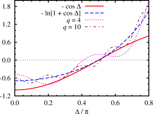
Figure 1: (Color online) Comparison beteween the singular model $V$, its regular counterpart, and some truncated expansions [Eqs. (3a), (4a), (5a)], as functions of the angle $\Delta$ between the two spins. Meaning of symbols: red continuous line: regular counterpart; blue dashed line: model $V$; magenta dotted line: $\mathcal{V}_{4}$; brown dash-dotted line: $\mathcal{V}_{10}$.

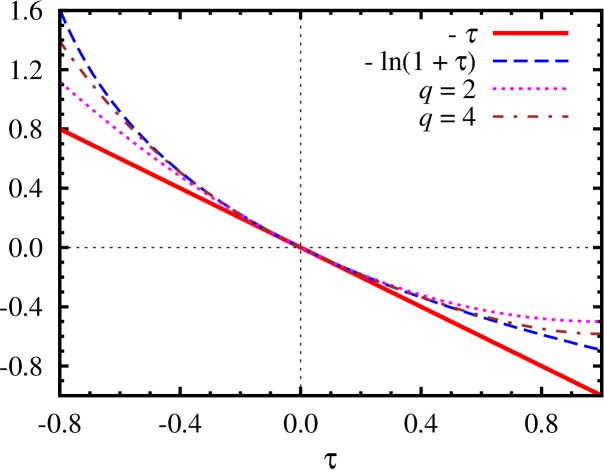
Figure 2: (Color online) Comparison beteween the singular model $W$, its regular counterpart, and some truncated expansions [Eqs. (3b), (4b), (5b)], as functions of the scalar product $\tau$ between the two spins. Meaning of symbols: red continuous line: regular counterpart; blue dashed line: model $W$; magenta dotted line: $\mathcal{W}_{2}$; brown dassh-dotted line: $\mathcal{W}_{4}$.

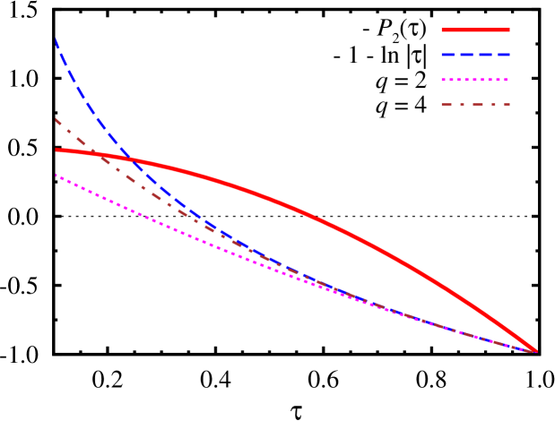
Figure 3: (Color online) Comparison beteween the singular model $X$, its regular counterpart, and some truncated expansions [Eqs. (3c), (4c), (5c)], as functions of the scalar product $\tau$ between the two spins. Meaning of symbols: red continuous line: regular counterpart; blue dashed line: model $X$; magenta dotted line: $\mathcal{X}_{2}$; brown dash-dotted line: $\mathcal{X}_{4}$. Notice that the quantity $-1$ has been added to $X$ as well as to the two truncated expansions, in order to ease comparison.

What happens when the underlying lattice is taken to be 2-dimensional? The functional forms under investigation here [Eqs. (3)] diverge to $+\infty$ for some mutual orientations, and, on the other hand, Refs. Ioffe et al. (2002); Gagnebin and Velenik (2014) address the general case of continuous functions of the scalar product and Ref. Ioffe et al. (2002) can even allow for some singularities; as far as we could check, the divergent behavior of the models under investigation here does not fit into the framework of weak singularity conditions used in section 2.2 of Ref. Ioffe et al. (2002). More explicitly, based on the series expansion in Eq. (5a), one could try to realize a decomposition of $V(\tau)$ along the lines of Ref. Ioffe et al. (2002), (sect. 2.2, around their Eqs. (24) to (26), page 441–443), by choosing a (large) positive integer $q$ and rewriting Eq. (3a) as

$$V(\tau)=\ln(2)+\mathcal{V}_{q}+r_{q};$$ (9)

the divergent term $r_{q}$ would then be positive around $\Delta=\pi$, and its sign would not agree with the hypotheses stipulated for theorem 1, singular case, in Ref. Ioffe et al. (2002), where the small singular term in the interaction is written (their notation)

$$-v(\phi),~{}v(\cdot)\geq 0.$$

Thus there appears to be no available mathematical theorem entailing a Mermin-Wagner-type result in this case, although it has been conjectured (expectation is not calculation) that, in the thermodynamic limit, orientational order is also destroyed at all finite temperatures; (see. e.g. Ref. 13 in Ref. Parameswaran et al. (2009)); on the other hand, at least for the $V$ case, one might expect a BKT behavior, since the singularity of the potential should ultimately strengthen short-range correlations.

III Simulation aspects and finite–size scaling theory

For $D=2$, the three models $V$, $W$ and $X$ [Eqs. (3)] were treated by simulation. Calculations were carried out using periodic boundary conditions, and on samples consisting of $N=L^{2}$ particles, with $L=40,60,80,100,120,160$. Simulations, based on standard Metropolis updating algorithm, were carried out in cascade, in order of increasing temperature $T$; equilibration runs took between 25000 and 50000 cycles, where one cycle corresponds to $2N$ attempted Monte Carlo steps, including sublattice sweeps (checkerboard decomposition Greeff and Lee (1994); Romano (1995); Hashim and Romano (1999); Binder and Heermann (2010)), and production runs took between 500000 and 1500000.

Subaverages for evaluating statistical errors were calculated over macrosteps consisting of 1000 cycles. Calculated quantities include the potential energy (in units $\epsilon$ per particle), and derivative with respect to temperature based on the fluctuation formula

$$U^{*}=\frac{\langle H\rangle}{N},$$ (10)

and

$$C^{*}=\frac{1}{NT^{2}}\left(\langle H^{2}\rangle-\langle H\rangle^{2}\right),$$ (11)

with

$$H=\sum_{\left\{j<k\right\}}F(\tau_{jk}),$$ (12)

where $\sum_{\left\{j<k\right\}}$ denotes sum over all distinct nearest–neighbouring pairs of lattice sites.

As for orientational quantities, such as mean magnetization and corresponding susceptibilities Paauw et al. (1975); Peczak et al. (1991), they can be expressed in general by

$$\mathbf{P}=\sum_{k=1}^{N}\mathbf{w}_{k},$$ (13a)

$$M=\frac{1}{N}\langle|\mathbf{P}|\rangle,$$ (13b)

$$M_{2}=\frac{1}{N}\langle\mathbf{P}\cdot\mathbf{P}\rangle,~{}$$ (13c)

$$\chi_{1}=\left\{\begin{array}[]{ll}\beta\left(M_{2}-NM^{2}\right),&T<T_{c}\\[14.22636pt] \beta M_{2},&T\geq T_{c}\end{array}\right.,$$ (14a)

where $$\beta=1/T T_{c} |\mathbf{P}|\leq N$$, and denotes the critical temperature; since [Eq. (13a)], we have

$$M_{2}\leq N\quad\mathrm{and}\quad~{}\chi_{1}\leq\beta N.$$ (14b)

Notice that Eq. (14a) involves a true ordering transition temperature $T_{c}$: in our case, for models $V$ and $W$, we found consistent evidence of the absence of orientational order at all finite temperatures (see also following Section), i.e. $T_{c}=0$, and selected the definition of $\chi_{1}$ accordingly. Model $X$ [Eq. (3c)], on the other hand, possesses even symmetry, and its second– and fourth–rank order parameters $\overline{P}_{2}$ and $\overline{P}_{4}$, as well as the corresponding susceptibility $\chi_{2}$, were calculated as discussed in Ref. Chamati and Romano (2008); notice that, in this case

$$\chi_{2}\leq\beta N.$$ (15)

We also calculated various short–range order parameters, defined by

$$\sigma_{J}=\langle\mathcal{E}_{J}(\tau_{jk})\rangle,$$ (16)

measuring correlations between corresponding pairs of unit vectors associated with nearest–neighbouring sites; here $\mathcal{E}_{J}(\tau)$ denote appropriate orthogonal polynomials [see Eq. (27) in Appedix A], and we chose $J=1,2$ for both $V$ and $W$ models, and $J=2,4$ for the $X$ model.

In the quest for the possible occurrence of a phase transition in the models investigated here, we will analyse the simulations data via the finite–size scaling (FSS) theory for continuous phase transitions – second order and BKT (infinite order) Binder and Heermann (2010); Newman and Barkema (1999); Chamati (2013). According to FSS hypothesis when a system is restricted to a finite geometry (a square of area $L^{2}$ in the present case) its thermodynamic quantities acquire a size dependence with a behavior that is tightly related to the order of the phase transition. It is worth mentioning that finite-size effects become important when the correlation length is of the same order as the linear size of the system. To be more specific we give details based on the behavior of the susceptibility.

In the vicinity of a bulk critical point $T_{c}$ the (magnetic) susceptibility diverges against the reduced temperature $t=1-\tfrac{T}{T_{c}}\ll 1$ according the scaling law $\chi_{1}\sim|t|^{-\gamma}$ with the critical exponent $\gamma>0$. For a finite-size system it turns into

$$\chi_{1}(L,T)=L^{\gamma/\nu}\Theta_{\chi}(tL^{1/\nu}),$$ (17)

where $\nu$ measures the degree of divergence of the distance over which the spins are correlated, i.e. the correlation length $\xi\sim|t|^{-1/\nu}$ with $\nu>0$. The function $\Theta_{\chi}(x)$ is a universal function depending on the gross features of the system, but not of its microscopic details.

On the other hand, when a BKT transition takes place, the susceptibility of the bulk system diverges exponentially

$$\chi_{BKT}\sim a_{\chi}\exp\left[b_{\chi}\left(T-T_{BKT}\right)^{-\tfrac{1}{2}}\right],\quad T_{BKT}\lesssim T$$ (18)

as we approach $T_{BKT}$ and is infinite in the BKT phase with a quasi–long range order. For a finite system however the divergence is rounded and the susceptibility is finite [Eqs. (14b) and (15)]. In the vicinity of the bulk BKT temperature the correlation length is proportional to the system’s linear size and the susceptibility scales like

$$\chi_{BKT}\sim L^{2-\eta_{BKT}(T)}.$$ (19)

At the transition temperature $\eta_{BKT}=\tfrac{1}{4}$.

Expressions (17) and (19) are valid asymptotically in the vicinity of the transition temperature i.e. when both the sample size $L$ and the correlation length $\xi$ are very large, but their ratio $\tfrac{\xi}{L}$ is finite. In this limit the universal scaling behavior is not affected by the finite-size effects.

IV Simulation results and FSS analysis

Simulation results obtained for the three investigated models turned out to exhibit broad qualitative similarities, to be contrasted to their regular counterparts (see following discussion).

IV.1 The magnetic models $V$ and $W$

Simulation results for various observables, obtained for the two models $V$ and $W$, were found to exhibit a recognizable qualitative similarity over a wide temperature range, so that, in some cases, only $V$ results will be presented in the following.

Simulation data for the potential energies of both models (not shown here) were found to evolve with tempereture in a gradual, monotonic way, and to be essentially independent of sample sizes, to within statistical errors falling below $0.1\%$.

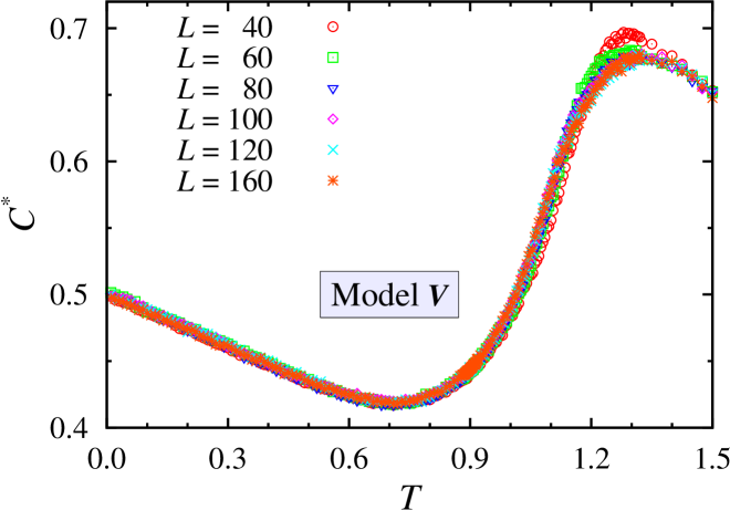
Figure 4: (Color online) The specific heat of model $V$ for different sample sizes against temperature; statistical errors (not shown here) range between $1$ and $5\%$. Meaning of symbols: red circles: $L=40$; green squares: $L=60$; blue triangles: $L=80$; magenta diamonds: $L=100$: cyan crosses, red asterisks: $L=160$.

As for the configurational specific heat $C^{*}$ (see FIG. 4 for model $V$, and FIG. 5, for model $W$), related to thermal fluctuations of the potential energy, the plots showed that $C^{*}$ starts with a maximum at $T=0$, and first decreases to a broad minimum (say at $T^{\prime})$; it then increases to another maximum (say at $T^{\prime\prime}$); here the associated statistical errors range between $1$ and $5\%$, and results are only mildly affected by sample size. We found $T^{\prime}\approx 0.75,~{}T^{\prime\prime}\approx 1.2$ for the $V$ model, and $T^{\prime}\approx 0.4,~{}T^{\prime\prime}\approx 0.62$ for the $W$ counterpart; upon extrapolating the low–temperature results to $T=0$, we estimate the corresponding zero–temperature values to be $\tfrac{1}{2}$ and $1$, respectively; notice also that the zero–temperature value for the $W$ model (but not for the $V$ model) corresponds to the global maximum; on the other hand, $T^{\prime\prime}$ for the $V$ model (but not for the $W$ model) corresponds to the global maximum. The same behaviour was found by estimating the specific heat via numerical differentiation of the internal energy.

Figure 5: (Color online) The specific heat of model $W$ for different sample sizes against temperature; statistical errors (not shown here) range between $1$ and $5\%$; same meaning of symbols as in FIG. 4.

A finite-size analysis of the configurational specific heat according to corresponding scaling behavior compatible with (17) ruled out the existence of a second order phase transition in both models. A similar analysis was performed on the magnetization and the susceptibility for both models, but no scaling was achieved.

Simulation results for the magnetization obtained with both models (see e.g. FIG. 6 for model $V$) showed a decreasing behavior as a function of temperature for a given sample size; at each examined nonzero temperature, they kept decreasing with increasing sample size; low–temperature results appear to extrapolate to $M=1$ at $T=0$ for all examined sample size, as expected.

Low–temperature simulation results for $M$ and for both models $V$ and $W$ were found to exhibit a power–law decay with increasing sample size; recall that the spin–wave analysis worked out in Ref. Tobochnik and Chester (1979) for the regular counterpart [Eq. (4a)] predicts the low–temperature result

$$M\approx\left(2L^{2}\right)^{-\tfrac{T}{8\pi}}.$$ (20)

Our data at a given temperature were well fitted in a log-log scale by the relation

$$\ln M=-a\ln L+b,\qquad~{}a>0,$$ (21)

where the ratio $\tfrac{a(T)}{T}$ was found to increase with temperature, and to become constant in the low–temperature limit.

Figure 6: (Color online) Simulation results for the magnetisation of model $V$ obtained with different sample sizes; same meaning of symbols as in FIG. 4.

The thermal fluctuations of the magnetization for both models $V$ and $W$ i.e. their magnetic susceptibilities (actually $\ln\chi_{1}$) are presented in FIGs. 7 and 8. At low temperatures the susceptibility keeps growing with sample size for both models, within the constraint of (14b), whereas at higher temperatures it becomes independent of sample size; the temperatures $T_{ch}$ where this change of scaling behavior first becomes recognizable are $T_{ch}\approx 1.3>T^{\prime\prime}$ for model $V$, and $T_{ch}\approx 0.56<T^{\prime\prime}$ for model $W$, respectively.

This specific behavior suggests a BKT transition from a quasi-long range ordered phase at low temperatures to a disordered phase at higher ones. Assuming such a transitional behavior, we have fitted the data of the largest sample size ($L=160$) to expression (18) for the bulk susceptibility and found the results of Table 1, as crude estimates (see also below).

Figure 7: (Color online) Simulation results for the susceptibility $\chi_{1}$ of model $V$ obtained with different sample sizes; same meaning of synbols as in FIG. 4; Assuming a BKT transition and fitting the largest sample size $L=160$ (upper continuous orange curve) to the bulk behavior of the susceptibility leads a transition at $T_{BKT}=0.883\pm 0.007$.

Figure 8: (Color online) Simulation results for the susceptibility $\chi_{1}$ of model $W$ obtained with different sample sizes; same meaning of symbols as in FIG. 4.

Table 1: Estimates of the parameters in Eq. (18) obtained by fitting to data for the largest sample size for models $V$, $W$ and $X$ assuming they exhibit a BKT transition.

Model	$\ln(a_{\chi})$	$b_{\chi}$	$T_{BKT}$
V	$-3.21\pm 0.15$	$5.29\pm 0.15$	$0.873\pm 0.007$
W	$-3.93\pm 0.14$	$5.40\pm 0.14$	$0.259\pm 0.007$
X	$-2.33\pm 0.05$	$3.03\pm 0.04$	$0.347\pm 0.003$

We analyzed the behavior of the susceptibility $\chi_{1}$ according to the finite-size scaling ansatz (19) in the vicinity of $T=0.9$ for model $V$ and of $T=0.28$ for model $W$; we first carried out a linear fit of $\ln\chi_{1}$ vs. $\ln L$ and estimated the critical exponent $\eta$ from the slope of the curves corresponding to different temperatures. The values obtained are presented in Tables 2 and 3, for models $V$ and $W$, respectively. A nonlinear fit, based on Eq. (19) was performed as well, and yielded results in agreement with these ones. Thus the transition temperatures are most likely at $T_{BKT}=0.910\pm 0.005$ and $T_{BKT}=0.275\pm 0.005$ for models $V$ and $W$, respectively. The discrepancy between these values and those in Table 1 points to the presence of huge finite-size effects: recall that Eq. (18) holds in the thermodynamic limit only, but was applied here to the largest investigated sample size in the hope to gain insights in the transitional behavior of the models considered here.

For the regular counterpart of model $V$ the configurational specific heat was found to exhibit a sharp maximum at about 15% Tobochnik and Chester (1979) above the BKT transition. In Refs. Chamati and Romano (2006, 2007) we have investigated the impact of diluted random impurities on the transition temperature. In Ref. Chamati and Romano (2006) we have found a broad peaks about 5% above the BKT transition, and in Ref. Chamati and Romano (2007) we found a sharper one about 2% above the transition temperature. Here we find a maximum at about 40% above $T_{BKT}$. All these results show that the maximum of the specific heat is always above the transition temperature. As for $T_{ch}$, we could not find in the Literature any estimate for the regular counterpart [Eq. (4a)]; thus additional simulations were run for the named regular model, carried out with the same sample sizes as for the three singular models, and using overrelaxation Fernández and Streit (1982); Gupta et al. (1988); Li and Teitel (1989); Gupta and Baillie (1992); Kadena and Mori (1994); the estimate $T_{ch}\approx 1.05$ was obtained.

Table 2: Estimates of $\eta$ for model $V$ obtained via a log-log fit according to Eq. (19) for different temperatures along with the corresponding error $\delta\eta$.

$T$	0.890	0.895	0.900	0.905	0.910	0.915	0.920
$\eta$	0.246	0.244	0.248	0.240	0.250	0.251	0.257
$\delta\eta$	0.007	0.006	0.006	0.006	0.005	0.004	0.006

Table 3: Estimates of $\eta$ for model $W$ obtained via a log-log fit according to Eq. (19) for different temperatures along with the corresponding error $\delta\eta$.

$T$	0.265	0.270	0.275	0.280	0.285	0.290	0.295
$\eta$	0.239	0.243	0.249	0.257	0.271	0.273	0.285
$\delta\eta$	0.004	0.004	0.004	0.006	0.006	0.005	0.007

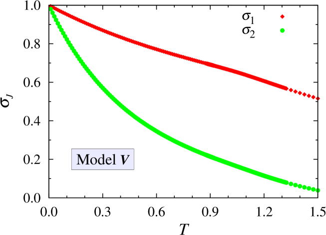
Figure 9: (Color online) Simulation results for the short-range order parameters (16) of model $V$ obtained with the largest sample size; meaning of symbols: red diamonds (upper curve) $\sigma_{1}$; green circles (lower curve): $\sigma_{2}$.

Simulation data for the short–range order parameters defined in (16) were found to be independent of sample size, and to decrease with temperature in a gradual and continuous way, paralleling the potential energy data; results obtained with the largest sample size of model $V$ are collected on FIG. 9.

IV.2 The two-dimensional nematic model $X$

Simulation results for the $X$ model were also found to exhibit a remarkable qualitative similarity with the ones obtained for their magnetic counterparts. Data for the potential energy (not shown) as well as for the short–range order parameters (FIG. 10) were found to be independent of sample size, and to evolve with temperature in a gradual and monotonic way. The temperature dependence of the specific heat corresponded to its magnetic counterpart (FIG. 11); here also the associated statistical errors were found to range between $1$ and $5\%$, and the results appeared to be only mildly affected by sample size. The plot started with the value $1$ at $T=0$, decreased with increasing temperature reaching a broad minimum at $T^{\prime}\approx 0.3$, and then its global maximum at $T^{\prime\prime}\approx 0.5$. it is worth mentioning that a quite similar behavior was obtained by numerical differentiation of the potential energy. Notice also that, in the three cases, sample–size effects on the results become more pronounced about $T^{\prime\prime}$. Here we anticipate that neither the results for the specific heat nor those corresponding to the second–rank order parameter $\overline{P}_{2}$ or to the susceptibility $\chi_{2}$ could obey the scaling behavior characteristic of a second order phase transition.

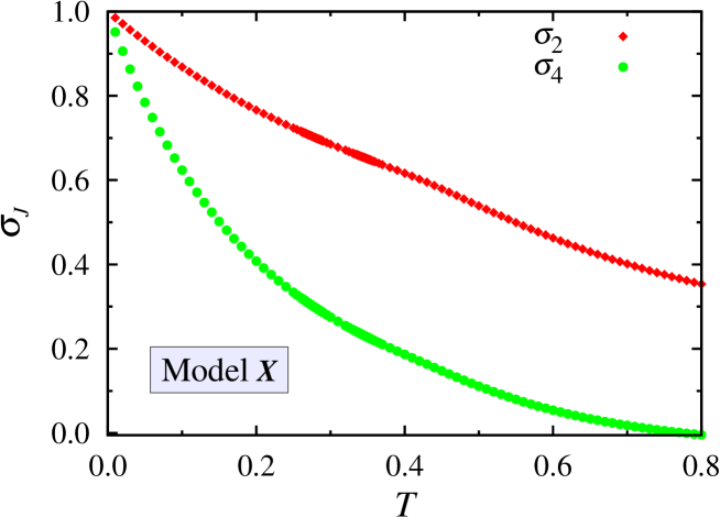
Figure 10: (Color online) Simulation results for the short-range order parameters (16) of model $X$ obtained with the largest sample size; meaning of symbols: red diamonds (upper curve) $\sigma_{2}$; green circles (lower curve): $\sigma_{4}$.

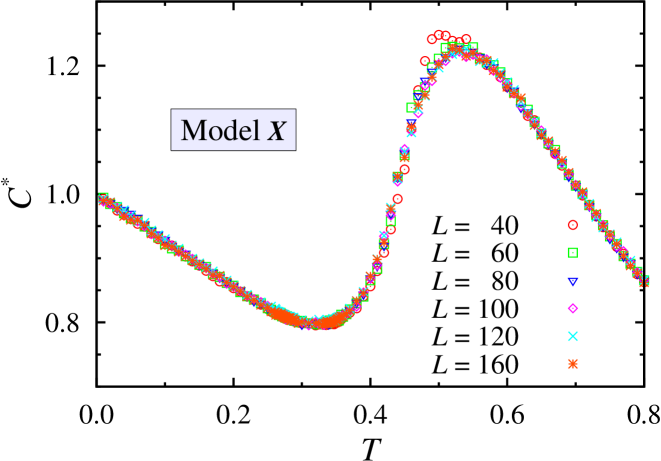
Figure 11: (Color online) The specific heat of model $X$ for different sample sizes against temperature; statistical errors (not shown here) range between $1$ and $5\%$; same meaning of symbols as in FIG. 4.

Simulation results for the order parameters $\overline{P}_{J}$, ($J=2,4$) were also found to decrease with increasing temperature for each sample size, and to decrease with increasing sample size at each nonzero temperature (FIG. 12 and FIG. 13). At all investigated temperatures the results for the nematic order parameters $\overline{P}_{M}$, ($M=2,4$) exhibited a power–law decay with increasing sample size. At a given temperature these were well fitted to the corresponding relations

$$\ln\overline{P}_{J}=-b_{J1}\ln L+b_{J0},\qquad~{}b_{J1}>0.$$ (22)

The coefficients $b_{J1}(T)$ were found to increase with $T$, and to become proportional to $T$ to within statistical errors in the low temperature region. The results obtained from Eq. (22) show that both order parameters vanish in the thermodynamic limit i.e. $L\to\infty$; such a behavior is in agreement with the spin wave theory for magnetic systems discussed above.

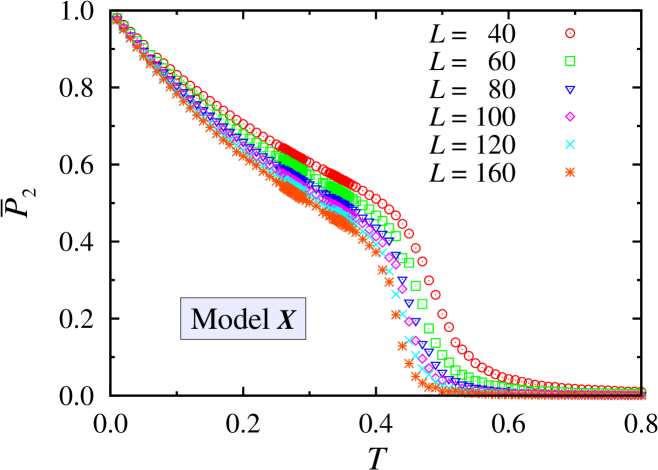
Figure 12: (Color online) Simulation results for the second–rank order parameter $\overline{P}_{2}$ of model $X$ obtained with different sample sizes; same meaning of symbols as in FIG. 4.

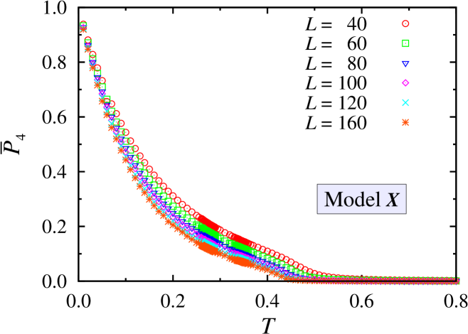
Figure 13: (Color online) Simulation results for the fourth–rank order parameter $\overline{P}_{4}$ of model $X$ obtained with different sample sizes; same meaning of symbols as in FIG. 4.

Simulation results for $\ln\chi_{2}$ versus $T$ (FIG. 14) showed a low-temperature regime where they kept increasing with increasing sample size, and then became independent of sample size at higher temperatures; the temperature $T_{ch}$ where this change of scaling first becomes recognizable was $T_{ch}\approx 0.45<T^{\prime\prime}$; this behavior also parallels the one observed for the two magnetic counterparts.

By fitting the data obtained at high temperatures for our largest sample size ($L=160$) to expression (18) of the susceptibility, we obtain the results reported in Table 1 with a transition temperature $T_{BKT}=0.347\pm 0.003$.

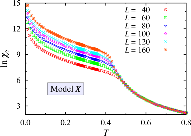
Figure 14: (Color online) Simulation results for the susceptibility $\chi_{2}$ of model $X$ obtained with different sample sizes; same meaning of symbols as in FIG. 4.

Upon applying the finite–size–scaling analysis with data for all sample sizes to the susceptibility given by Eq. (19), we end up with the results of Table 4 with an estimate of the transition temperature $\Theta_{BKT}=0.275\pm 0.005$ for model X. Here again we observe a discrepancy between the result obtained by fitting the bulk expression of the susceptibility to the data for the largest size and the FSS analysis. This may be traced back to the huge finite-size effects.

Table 4: Estimates of $\eta$ for Model $X$ obtained via a log-log fit according to Eq. (19) for different temperatures along with the corresponding error $\delta\eta$.

$T$	0.260	0.265	0.270	0.275	0.280	0.285	0.290
$\eta$	0.237	0.243	0.248	0.250	0.258	0.266	0.269
$\delta\eta$	0.006	0.005	0.005	0.006	0.004	0.006	0.003

IV.3 Comparisons with the regular counterparts

As for the regular counterparts [Eqs. (4)], the existence of a BKT transition is by now a well-known result for planar rotators [Eq. (4a)], and an estimate of the transition temperature to be found in the Literature is $T_{BKT}=0.8929\pm 0.0001$ Hasenbusch (2008); Arisue (2009); $T_{BKT}$ found for the $V$ model is about $2\%$ higher than the corresponding value for the regular counterpart.

On the other hand, available evidence does not seem to support a BKT scenario for the classical $O(3)$ Heisenberg regular counterpart [Eq. (4b)]. Various authors (see, e.g., Ref. Butera et al. (1990)) have argued that the model does not exhibit such a transition; the opposite view has been put forward by Patrascioiu and Seiler, in a series of papers (see e.g. Patrascioiu and Seiler (2002); *Patrascioiu1991173); examples of the resulting debate can be found in or via Refs. Tomita (2014).

The nematic case [Eq. (4c)] has been studied for some 30 years Solomon (1981); Sinclair (1982); Fukugita et al. (1982); Chiccoli et al. (1988); Kogan et al. (1990); Khveshchenko et al. (1991); Kunz and Zumbach (1989); *Kunz1991299; *PhysRevB.46.662; Butera and Comi (1992); Caracciolo et al. (1993); Mukhopadhyay and Roy (1997); Bulgadaev (2001); Mondal and Roy (2003), and a BKT scenario has been proposed by various Authors: a recent estimate of the transition temperature is $T_{BKT}=0.548\pm 0.002$ Mondal and Roy (2003), with the $C^{*}$ maximum at $T^{\prime\prime}\approx 0.57$, and $T_{ch}\approx T^{\prime\prime}$; on the other hand, some other Authors claim that the named model [Eq. (4c)] does not exhibit any critical transition, but its low–temperature behavior is rather characterized by a crossover from a disordered phase to an ordered phase at zero temperature Paredes et al. (2008); Fariñas Sánchez et al. (2010).

Table 5: A summary of characteristic temperatures for the three models examined by simulation in the present work; see text for definitions.

Model	$T^{\prime}$	$T^{\prime\prime}$	$T_{ch}$	$T_{BKT}$
V	$\approx 0.75$	$\approx 1.25$	$\approx 1.3$	$0.910\pm 0.005$
W	$\approx 0.4$	$\approx 0.62$	$\approx 0.56$	$0.275\pm 0.005$
X	$\approx 0.3$	$\approx 0.5$	$\approx 0.45$	$0.275\pm 0.005$

These comparisons (see also Table 5) suggest that, on the one hand, the singular character of the interaction may bring about a BKT behavior where the regular counterpart does not support it (W model); on the other hand, the effect on $T_{BKT}$ appears to be milder where the regular counterparts already support this transitional behavior, and this we interpret as a reflection of the potential features pointed out previously (Sect. II), in the discussion of Eqs. (5) and of FIGS. 1, 2 and 3.

In contrast to the regular counterparts, where the temperature dependence of $C^{*}$ shows a simple maximum, upon increasing temperature from $T=0$, the three singular models investigated here exhibit first a minimum and then a maximum of $C^{*}$; this behavior also appears connected with the potential features discussed in Sect. II.

V Summary and conclusions

We have revisited and generalized a previously studied model Niemeijer and Ruijgrok (1977); Ishimori (1982) and defined a few others, whose pairwise interactions are isotropic in spin space and restricted to nearest neighbours; in contrast to other extensively studied models, their functional forms contains logarithmic singularities which, so to speak, do not disturb the thermodynamics. When $D=1$, the above models could be solved in closed form, in terms of Gamma, Beta and Polygamma functions, and were found to produce orientational disorder and no phase transition, at all finite temperatures, in the thermodynamic limit. Some of the above models have been studied by simulation for $D=2$: among a few candidates (see Section II), we had chosen those functional forms which strongly favour mutual parallel orientations, thus strengthening (at least) short–range correlations; in the absence of more stringent rigorous results, the obtained simulation results point to orientational disorder at all finite temperatures, and suggest a BKT scenario in the three cases; we hope to carry out a more thorough simulation study of the models.

Moreover, the investigated models contain logarithmic singularities, causing them to slowly diverge as $\tau\rightarrow-1$ or $\tau\rightarrow 0$; on the other hand, comparison with the regular counterparts and with the above constrained models (Section II) leads one to speculate as to what happens if the interaction potential is chosen to be more confining, i.e. made more rapidly divergent as $\tau$ moves away from $\tau_{min}$ (actually, a multitude of such functional forms can be envisaged); preliminary work along these lines has been started, and its results will be reported in due course.

Appendix A Exact solutions for $D=1$

Some available exact results in one dimension are recalled here; when $D=1$ (hence $\mathbf{x}_{j}\equiv j\in\mathbb{Z}$), for a linear sample consisting of $N$ spins, the Hamiltonian reads

$$H=\sum_{j=1}^{N}F\left(\mathbf{w}_{j}\cdot\mathbf{w}_{j+1}\right),$$ (23)

where we assume periodic boundary conditions i.e. $\mathbf{w}_{N+1}=\mathbf{w}_{1}$; the corresponding overall partition functions can be calculated exactly, and this is usually realized based on the underlying $O(n)$ symmetry, by means of an appropriate coordinate transformation (i.e., geometrically, by taking each spin $\mathbf{w}_{j}$ as defining the reference axis for the next one $\mathbf{w}_{j+1}$) Fisher (1964); Joyce (1967); Stanley (1969); Thompson (1972); Freasier (1973); Vuillermot and Romerio (1973); the corresponding overall partition function reduces to the $N-$th power [or $(N-1)-$th power if one uses free boundary conditions] of a single-particle quantity, to be denoted here by $q(T)$; in formulae

$$q(T) = \frac{1}{2\pi}p(T),$$ (24a)

$$p(T) = \int_{0}^{2\pi}\exp(-\beta F(\cos s))ds,\quad n=2,$$ (24b)

and

$$q(T) = \frac{1}{2}p(T),$$ (25a)

$$p(T) = \int_{-1}^{+1}\exp(-\beta F(s))ds,\quad n=3,$$ (25b)

where $\beta=1/T$; correlation functions are defined by

$$G_{J}(m)=\langle\mathcal{E}_{J}(\mathbf{w}_{j}\cdot\mathbf{w}_{k})\rangle,~{}\mathrm{as~{}function~{}of}~{}m=|\mathbf{x}_{j}-\mathbf{x}_{k}|;$$ (26)

here $J$ is a strictly positive integer, and $\mathcal{E}_{J}(\tau)$ denote appropriate orthogonal polynomials, i.e.

$$\mathcal{E}_{J}(\tau)=\left\{\begin{array}[]{ll}T_{J}(\tau)=\cos(J\arccos(\tau)),&~{}n=2\\[9.95863pt] P_{J}(\tau),&~{}n=3\end{array}\right.;$$ (27)

here $T_{J}(\ldots)$ denote Chebyshev polynomials of the first kind, and $P_{J}(\ldots)$ denote Legendre polynomials. For general $D$, and when $F(\tau)$ is not an even function of its argument, the simplest correlation function is $G_{1}(r)$; for $D=1$, the definition in Eq. (26) simplify to

$$G_{J}(m)=\langle\mathcal{E}_{J}(\mathbf{w}_{j}\cdot\mathbf{w}_{k})\rangle,~{}\mathrm{as~{}function~{}of}~{}m=|j-k|;$$ (28)

and $G_{1}(m)$ reduces to the $m-$th power of the quantity

$$c_{1}(T)=\frac{r_{1}(T)}{p(T)},$$ (29)

where

$$r_{1}(T) = \int_{0}^{2\pi}\cos s\exp(-\beta F(\cos s))ds,~{}n=2,$$ (30a)

$$r_{1}(T) = \int_{-1}^{+1}s\exp(-\beta F(s))ds,\quad n=3.$$ (30b)

The corresponding susceptibility is given by Paauw et al. (1975); Peczak et al. (1991) [see also the following Eqs. (13c) and (14a)]

$$\chi_{1} = \frac{\beta}{N}\left\langle\sum_{j=1}^{N}\sum_{k=1}^{N}(\mathbf{w}_{j}\cdot\mathbf{w}_{k})\right\rangle$$ (31)

$$= \frac{\beta}{N}\sum_{j=1}^{N}\sum_{k=1}^{N}G_{1}(|j-k|)$$

$$= \frac{\beta}{N}\sum_{j=1}^{N}\sum_{k=1}^{N}c_{1}^{|j-k|};$$

hence, in the large–$N$ limit,

$$\chi_{1}=\beta\frac{1+c_{1}}{1-c_{1}}.$$ (32)

These quantities have been calculated in the Literature in a few cases, where $F(\tau)$ is a simple polynomial of its argument. i.e. $F=\pm\tau~{}(n=2,3),~{}F=\pm P_{2}(\tau)~{}(n=3)$ Fisher (1964); Joyce (1967); Stanley (1969); Thompson (1972); Freasier (1973); Vuillermot and Romerio (1973); Hashim and Romano (1998); in the latter cases $F(\tau)$ is an even function of its argument, so that the simplest relevant correlation function is

$$G_{2}(m)=\langle P_{2}(\mathbf{w}_{j}\cdot\mathbf{w}_{k})\rangle,~{}\mathrm{as~{}function~{}of}~{}m=|j-k|,$$ (33)

which similarly reduces to the $m-$th power of

$$c_{2}(T) = \frac{r_{2}(T)}{p(T)},$$ (34a)

$$r_{2}(T) = \int_{-1}^{+1}P_{2}(s)\exp(-\beta F(s))ds,\quad n=3;$$

in the large–$N$ limit, the corresponding susceptibility reads

$$\chi_{2}=\beta\frac{1+c_{2}}{1-c_{2}}.$$ (35)

Notice that the continuity of $F(\tau)$ implies convergence and regularity of $q(T)$; moreover the definitions entail $|c_{1}(T)|<1$ or $|c_{2}(T)|<1$ at all finite temperatures; thus leading to the well known results related to the absence of phase transitions at all finite temperatures, orientational disorder in the thermodynamic limit at all finite temperatures, and exponential decay with distance for the absolute value of the correlation functions; actually, these results may also hold under weaker conditions on $F(\tau)$.

There also exist in the literature a few lattice–spin models involving mild integrable singularities, i.e. defined by bounded and generally continuous functions of the scalar products, which still allow usage of the method outlined here when $D=1$; one such case is the sign or step model Guttmann et al. (1972); Guttmann and Joyce (1973); Lee and Shrock (1987, 1988); Irving and Kenna (1996); Kenna and Irving (1997); Olsson and Holme (2001), defined by

$$F(\tau)=\pm\ \mathrm{sign}(\tau);$$ (36)

the model was solved exactly for $D=1$ and $n\geq 2$ Lee and Shrock (1987), and proven to remain orientationally disordered even at $T=0$, where calculations in Ref. Lee and Shrock (1987) yield for the ferromagnetic case

$$G_{1}(1)=\frac{1}{\sqrt{\pi}}\,\frac{\Gamma(n/2)}{\Gamma((n+1)/2)};$$ (37)

for $D=n=2$ there is consistent evidence of orientational disorder at all temperatures, as well as of the existence of a BKT transition Irving and Kenna (1996); Kenna and Irving (1997); Olsson and Holme (2001).

We notice in passing that other extensions of Eq. (36) can be envisaged, e. g.

$$F(\tau)=\pm\mathrm{sign}(P_{J}(\tau)),~{}n=3,$$ (38)

where, say, $J=2,3,4$; when $D=1$, the resulting partition functions can be worked out in closed form as well.

The effect of divergences in $F(\tau)$ was seldom investigated, and we shall be considering here some extensions of Eqs. (3a) and (3b), in addition to Eq. (3c),

$$V_{I}(\tau) = -\ln(1+I\tau),\quad n=2,$$ (39a)

$$W_{I}(\tau) = -\ln(1+I\tau),\quad n=3,$$ (39b)

where $I=\pm 1$ defines the ferro- or antiferro-magnetic character of the interaction. Both $V_{I}(\tau)$ and $W_{I}(\tau)$ attain their minimum when $\tau=I$, and slowly diverge to $+\infty$ as $\tau\rightarrow-I$; $X(\tau)$ attains its minima when $\tau=\pm 1$ and slowly diverges to $+\infty$ as $\tau\rightarrow 0$; the above functions are bounded from below, continuous almost everywhere, and possess integrable singularities; moreover, their functional forms turn out to be computationally convenient for $D=1$. Two other related models can be defined as well, by combinining ferro– and antiferro–magnetic cases of $V_{I}(\tau)$ with equal positive weights, and similarly for $W_{I}(\tau)$; in formulae:

$$A_{2}(\tau) = -\ln(2(1-\tau^{2})),\quad n=2,$$ (40a)

$$A_{3}(\tau) = -\ln(1-\tau^{2}),\quad n=3.$$ (40b)

Both $A_{2}(\tau)$ and $A_{3}(\tau)$ are even functions of their argument, attaining their minimum for $\tau=0$ and diverging to $+\infty$ for $|\tau|\rightarrow+1$; the letter $A$ in the names recalls their antinematic character. Actually, further generalizations of the $V_{I}$ models are possible, i.e.

$$V_{I,K}(\tau)=-\ln(1+I\cos(K\Delta_{jk})),\quad n=2$$ (41)

where $K$ is an arbitrary, strictly positive, integer, and $V_{I,1}=V_{I}$. By now it has been known for some time that interaction models only differing in the value of $K$ produce the same partition functions, and that the resulting orientational properties can be defined in a way independent of $K$ Romano (2006); Carmesin (1987); Romano (1987); for more details see Appendix B. A few specific cases are listed here

$$V_{+1,1}(\tau) = -\ln(1+\cos(\Delta_{jk})),$$ (42a)

$$V_{-1,1}(\tau) = -\ln(1-\cos(\Delta_{jk})),$$ (42b)

$$V_{+1,2}(\tau) = -\ln(1+\cos(2\Delta_{jk})),$$ (42c)

$$V_{-1,2}(\tau) = -\ln(1-\cos(2\Delta_{jk})).$$ (42d)

The standard trigonometric identity

$$\cos(2x)=2\cos^{2}x-1$$

entails that

$$V_{+1,2}(\tau) = -\ln(2\cos^{2}\Delta_{jk}),$$ (42e)

$$V_{-1,2}(\tau) = -\ln(2\sin^{2}\Delta_{jk});$$ (42f)

one recognizes that $V_{+1,2}$ defines the $2-$component counterpart of the $X$ model, and that $V_{-1,2}$ essentially coincides with $A_{2}$.

The above models can be solved explicitly, as worked out in the following: notice also that some qualitative results can be obtained in a more direct and elementary way, e.g., for $V_{I,1}(\tau)$,

$$p(T) = \int_{0}^{2\pi}(1+I\cos s)^{\beta}ds$$

$$= \int_{-\pi/2}^{+\pi/2}\left[(1+\cos s)^{\beta}+(1-\cos s)^{\beta}\right]ds;~{}$$

and, for the correlation function,

$$r_{1}(T) = \int_{0}^{2\pi}\cos s(1+I\cos s)^{\beta}ds$$

$$= I\int_{-\pi/2}^{+\pi/2}\cos s\left[(1+\cos s)^{\beta}-(1-\cos s)^{\beta}\right]ds;$$

since $|\cos s|\leq 1$, the above equations entail $|c_{1}(T)|<1$ at all finite temperatures. A similar approach can be used $W_{I}(\tau)$, i.e.

$$p(T) = \int_{-1}^{+1}(1+Is)^{\beta}ds$$ (44a)

$$= \int_{0}^{+1}\left[(1+s)^{\beta}+(1-s)^{\beta}\right]ds;~{}$$

and, for the correlation function,

$$r_{1}(T) = \int_{-1}^{+1}s(1+Is)^{\beta}ds$$ (44b)

$$= I\int_{0}^{+1}s\left[(1+s)^{\beta}-(1-s)^{\beta}\right]ds;$$

since $|s|\leq 1$, the above equations entail $|c_{1}(T)|<1$ at all finite temperatures.

Notice that, for each of the two functional forms (39a) or (39b), and in the absence of an external field, the two possible choices for I define models producing the same partition functions and correlation functions related by appropriate numerical factors (equivalent by spin–flip symmetry).

The above models can be solved explicitly in terms of known special functions with well defined analytic properties, and some of them yield results involving the functions: Gamma

$$\Gamma(z)=\int_{0}^{+\infty}s^{z-1}\exp(-s)ds,$$

Beta

$$B(x,y)=B(y,x)=\frac{\Gamma(x)\Gamma(y)}{\Gamma(x+y)};$$

and Polygamma

$$\Psi(l,z)=\frac{d^{l+1}}{dz^{l+1}}\ln\Gamma(z).$$

Here $x,~{}y,~{}z$ are complex variables with $\Re(x)>0,~{}\Re(y)>0,\Re(z)>0$, and $l$ denotes a nonnegative integer Davis (1972); Gradshteyn and Ryzhik (2007); let us also recall that $\Gamma\left(\frac{1}{2}\right)=\sqrt{\pi}$.

The above properties of $V$ models read

$$p(T) = 2^{\beta}\int_{0}^{2\pi}(\cos^{2}s)^{\beta}ds$$

$$= 2^{\beta}\int_{0}^{2\pi}(\sin^{2}s)^{\beta}ds$$

$$= 2\sqrt{\pi}2^{\beta}\frac{\Gamma(\beta+\tfrac{1}{2})}{\Gamma(\beta+1)}$$ (45a)

$$q(T) = \frac{\sqrt{\pi}}{\pi}2^{\beta}\frac{\Gamma(\beta+\tfrac{1}{2})}{\Gamma(\beta+1)};$$ (45b)

the configurational specific heat (in units $$k_{B}$$ per particle) can be obtained via the appropriate derivatives of the partition function and reads

$$C^{*}=\frac{1}{T^{2}}\left[\Psi\left(1,\frac{1}{T}+\frac{1}{2}\right)-\Psi\left(1,\frac{1}{T}\right)\right]+1$$ (45c)

For $$V_{+1,2}$$

$$c_{2}(T)=\frac{\beta}{\beta+1},$$ (45d)

and in general for $$V_{I,K}$$

$$c_{K}(T)=I\frac{\beta}{\beta+1},$$ (45e)

notice that $c_{2}$ for $V_{+1,2}$ is the same as $c_{1}$ for $V_{+1,1}$.

The corresponding results for $W_{I}(\tau)$ are

$$q(T) = \frac{2^{\beta}}{\beta+1},$$ (46a)

$$C^{*} = \frac{1}{1+T^{2}},$$ (46b)

$$c_{1}(T) = I\frac{\beta}{\beta+2}.$$ (46c)

For $X(\tau)$ one finds

$$p(T)=\frac{2}{\beta+1},$$ (47a)

$$C^{*}=\frac{1}{1+T^{2}},$$ (47b)

$$X(\tau)$$ is an even function of its argument, and the previous Eqs. (34a) and (LABEL:eq05c) specialize to

$$c_{2}(T) = \frac{r_{2}(T)}{p(T)},$$ (47c)

$$r_{2}(T) = \int_{-1}^{+1}P_{2}(s)|s|^{\beta}ds,$$ (47d)

and eventually

$$q(T) = \frac{1}{\beta+1},$$ (47e)

$$c_{2}(T) = \frac{\beta}{\beta+3}.$$ (47f)

Notice also that both $W_{I}(\tau)$ and $X(\tau)$ yield the same expression for the configurational contribution to the specific heat per particle [Eqs. (46b) and (47b)], and produce rather similar expressions for $c_{1}$ [Eq. (46c)] and $c_{2}$ [Eq. (47f)], respectively. As for the four $V$ models in Eqs. (42), let us recall that models with the same $I$ and different $K$ produce the same partition functions, and their orientational properties can be defined in a way independent of $K$, i.e. $G_{m}(r)$ for $V_{I,1}$ is the same as $G_{2m}(r)$ for $V_{I,2}$ Romano (2006); Carmesin (1987); Romano (1987); on the other hand, the above calculations also show that $V_{+1,1}$ and $V_{-1,1}$ produce the same partition functions and correlation functions connected by appropriate sign factors; thus the four named interaction models [Eqs. (42)] produce one and the same partition function, and essentially the same orientational properties.

The corresponding properties for $A_{3}$ model can be obtained in closed form as well;

$$q(T)=\frac{\sqrt{\pi}}{2\pi}\frac{\Gamma(\beta+1)}{\Gamma(\beta+\tfrac{3}{2})}$$ (48a)

$$C^{*}=\frac{1}{{T}^{2}}\left[\Psi\left(1,1+\frac{1}{T}\right)-\Psi\left(1,\frac{3}{2}+\frac{1}{T}\right)\right]$$ (48b)

$$c_{2}(T)=-\frac{\beta}{2\beta+3}.$$ (48c)

Notice that one can combine the potential models $X$ and $A_{3}$ to define

$$Y(\tau)=-\ln[\tau^{2}(1-\tau^{2})],\quad~{}n=3;$$ (49)

in this case the interaction diverges to $+\infty$ when $\tau=0$ and $|\tau|=1$; on the other hand, by standard trigonometric identities, one can recognize that the $n=2$ counterpart corresponds to $V_{-1,4}$ within numerical factors. The partition function of model $Y$ is

$$q(T)=\frac{\sqrt{\pi}}{2}4^{-\beta}\frac{\Gamma(2\beta+1)}{\Gamma(2\beta+\tfrac{3}{2})},$$ (50a)

and the corresponding quantities are given by

$$C^{*}=\frac{4}{T^{2}}\left[\Psi\left(1,1+\frac{2}{T}\right)-\Psi\left(1,\frac{3}{2}+\frac{2}{T}\right)\right]$$ (50b)

$$c_{2}(T)=\frac{1}{4+3T}.$$ (50c)

In all of the above cases, $C^{*}$ was found to be a monotonic decreasing function of temperature, in contrast to the regular counterparts Eqs. (4a) and (4c), which produce a maximum of $C^{*}(T)$; on the other hand, Eq. (4b) also produces a monotonic decreasing behavior for $C^{*}(T)$.

In the main text we are simply referring to $V_{+1,1}$ as $V$ model, and to $W_{+1}$ as $W$ model. For $D=1$, the named models produce no phase transition and no orientational order at finite temperatures in the thermodynamic limit; actually, some non–integrable singularities in $F(\tau)$ can produce the same qualitative behavior as well; this happens, for example, with constrained models, defined as follows: let $s_{0}$ denote a real number, $0<s_{0}<\pi,~{}\tau_{0}=\cos s_{0}$, and let Ioffe et al. (2002); Patrascioiu and Seiler (1992); Aizenman (1994); Bietenholz et al. (2013)

$$F(\tau)=\left\{\begin{array}[]{l l}f(\tau)&,~{}+1\geq\tau>\tau_{0}\\[8.5359pt] +\infty&,~{}-1\leq\tau<\tau_{0}\end{array}\right.,$$ (51)

where $f(\tau)$ denotes some regular function of its argument (see also below); in other words, the absolute value of the angle between the two interacting unit vectors, defined modulo $2\pi$, is constrained to remain below the threshold $s_{0}$. Upon following the previous line of thought and applying Eqs. (24) to (30b), one can recognize that, when $D=1$, functional forms like Eq. (51) also produce no phase transition and no orientational order at finite temperatures in the thermodynamic limit. Models defined by Eq. (51) and $D=n=2$ have also been addressed: for $f(\tau)=-\tau$, it was proven that, when $s_{0}$ is sufficiently small, the correlation function $G_{1}(r)$ never decays exponentially with distance, but obeys an inverse–square lower bound at all temperatures Ioffe et al. (2002); Patrascioiu and Seiler (1992); Aizenman (1994); on the other hand, when $f(\tau)=0$ Bietenholz et al. (2013), the system is athermal, and there is a simulation evidence of a BKT transition with $s_{0}$ as control parameter.

Appendix B Mapping between potential models

Consider the integral

$$\psi=\int_{0}^{2\pi}\Phi(\cos s,\sin s)ds,$$ (52)

where $\Phi$ denotes a sufficiently regular function, and let

$$\Psi_{K}=\int_{0}^{2\pi}\Phi(\cos Ks,\sin Ks)ds,$$ (53)

where $K$ is an arbitrary non–zero integer, and $\Psi_{1}=\psi$; one can immediately verify that

$$\forall K\in\mathbb{Z}\setminus\{{0}\},\Psi_{K}=\psi;$$ (54)

consider now

$$\Xi=\int_{0}^{2\pi}\exp(\pm i\mu s)\Phi(\cos Ks,\sin Ks)ds,$$ (55)

where $\mu>1$ denotes an arbitrary positive integer, and recall the identity

$$\sum_{j=1}^{j=\mu}\exp\left(\pm 2\pi i\frac{j}{\mu}\right)=0.\quad\mu>1.$$ (56)

Thus the value of $\Xi$ in Eq. (55) is zero when $\mu$ is not an integer multiple of $K$; on the other hand, when $\mu$ is an integer multiple of $K$, say $\mu=\lambda K$, the value of $\Xi$ is again independent of $K$

References

- Mermin and Wagner (1966a) N. D. Mermin and H. Wagner, Phys. Rev. Lett. 17, 1133 (1966a).
- Mermin and Wagner (1966b) N. D. Mermin and H. Wagner, Erratum, ibid. 17, 1307 (1966b).
- Mermin (1969) N. D. Mermin, J. Phys. Soc. Japan 26 Suppl., 203 (1969).
- Mermin (1967) N. D. Mermin, J. Math. Phys. 8, 1061 (1967).
- Thorpe (1971) M. F. Thorpe, J. Appl. Phys. 42, 1410 (1971).
- Nenciu (1971) G. Nenciu, Phys. Lett. A 34, 422 (1971).
- Vuillermot and Romerio (1975) P.-A. Vuillermot and M. V. Romerio, Commun. Math. Phys. 41, 281 (1975).
- Gelfert and Nolting (2001) A. Gelfert and W. Nolting, J. Phys.: Condens. Matt. 13, R505 (2001).
- Sinaǐ (1982) Y. G. Sinaǐ, Theory of Phase Transitions: Rigorous Results (Pergamon, Oxford, 1982).
- Georgii (1988) H.-O. Georgii, Gibbs Measures and Phase Transitions, de Gruyter Studies in Mathematics, Vol. 9 (Walter de Gruyter, Berlin, 1988).
- Ioffe et al. (2002) D. Ioffe, S. Shlosman, and Y. Velenik, Commun. Math. Phys. 226, 433 (2002).
- Gagnebin and Velenik (2014) M. Gagnebin and Y. Velenik, Commun. Math. Phys. 332, 1235 (2014).
- Pfister (1981) C. E. Pfister, Comm. Math. Phys. 79, 181 (1981).
- Fröhlich and Pfister (1981) J. Fröhlich and C. Pfister, Commun. Math. Phys. 81, 277 (1981).
- Picco (1983) P. Picco, J. Stat. Phys. 32, 627 (1983).
- Picco (1984) P. Picco, J. Stat. Phys. 36, 489 (1984).
- van Enter and Fröhlich (1985) A. C. D. van Enter and J. Fröhlich, Commun. Math. Phys. 98, 425 (1985).
- van Enter (1985) A. C. D. van Enter, J. Stat. Phys. 41, 315 (1985).
- Fröhlich and Ueltschi (2015) J. Fröhlich and D. Ueltschi, J. Math. Phys 56, 053302 (2015).
- Fröhlich and Spencer (1981) J. Fröhlich and T. Spencer, Commun. Math. Phys. 81, 527 (1981).
- Minnhagen (1987) P. Minnhagen, Rev. Mod. Phys. 59, 1001 (1987).
- Pierson (1997) S. W. Pierson, Phil. Mag. B 76, 715 (1997).
- Gulácsi and Gulácsi (1998) Z. Gulácsi and M. Gulácsi, Adv. Phys. 47, 1 (1998).
- Romano (2006) S. Romano, Phys. Rev. E 73, 042701 (2006).
- José (2013) J. V. José, ed., 40 years of Berezinskii-Kosterlitz-Thouless Theory (World Scientific, Singapore, 2013).
- van Enter and Shlosman (2002) A. C. D. van Enter and S. B. Shlosman, Phys. Rev. Lett. 89, 285702 (2002).
- van Enter and Shlosman (2005) A. C. D. van Enter and S. B. Shlosman, Commun. Math. Phys. 255, 21 (2005).
- Niemeijer and Ruijgrok (1977) T. Niemeijer and T. Ruijgrok, Physica A 86, 200 (1977).
- Ishimori (1982) Y. Ishimori, J. Phys. Soc. Jpn. 51, 3417 (1982).
- Arovas et al. (1988) D. P. Arovas, A. Auerbach, and F. D. M. Haldane, Phys. Rev. Lett. 60, 531 (1988).
- Parameswaran et al. (2009) S. A. Parameswaran, S. L. Sondhi, and D. P. Arovas, Phys. Rev. B 79, 024408 (2009).
- Daniel and Manivannan (1998) M. Daniel and K. Manivannan, Phys. Rev. B 57, 60 (1998).
- Daniel and Manivannan (1999) M. Daniel and K. Manivannan, J. Math. Phys. 40, 2560 (1999).
- Costa and Pires (2001) B. V. Costa and A. S. T. Pires, Phys. Rev. B 64, 092407 (2001).
- Poderoso et al. (2011) F. C. Poderoso, J. J. Arenzon, and Y. Levin, Phys. Rev. Lett 106, 067202 (2011).
- Fariñas Sánchez et al. (2005) A. I. Fariñas Sánchez, R. Paredes, and B. Berche, Phys. Rev. E 72, 031711 (2005).
- Geng and Selinger (2009) J. Geng and J. V. Selinger, Phys. Rev. E 80, 011707 (2009).
- Greeff and Lee (1994) C. W. Greeff and M. A. Lee, Phys. Rev. E 49, 3225 (1994).
- Romano (1995) S. Romano, Int. J. Mod. Phys. B 9, 85 (1995).
- Hashim and Romano (1999) R. Hashim and S. Romano, Int. J. Mod. Phys. B 13, 3879 (1999).
- Binder and Heermann (2010) K. Binder and D. W. Heermann, Monte Carlo Simulation in Statistical Physics: An Introduction, 5th ed., Graduate Texts in Physics (Springer, 2010).
- Paauw et al. (1975) T. T. A. Paauw, A. Compagner, and D. Bedeaux, Physica A 79, 1 (1975).
- Peczak et al. (1991) P. Peczak, A. M. Ferrenberg, and D. P. Landau, Phys. Rev. B 43, 6087 (1991).
- Chamati and Romano (2008) H. Chamati and S. Romano, Phys. Rev. E 77, 051704 (2008).
- Newman and Barkema (1999) M. E. J. Newman and G. T. Barkema, Monte Carlo Methods in Statistical Physics (Oxford University Press, New York, 1999).
- Chamati (2013) H. Chamati, in A Tribute to Marin D. Mitov, Advances in Planar Lipid Bilayers and Liposomes, Vol. 17, edited by A. Iglič and J. Genova (Academic Press, New York, 2013) p. 237.
- Tobochnik and Chester (1979) J. Tobochnik and G. V. Chester, Phys. Rev. B 20, 3761 (1979).
- Chamati and Romano (2006) H. Chamati and S. Romano, Phys. Rev. B 73, 184424 (2006).
- Chamati and Romano (2007) H. Chamati and S. Romano, Phys. Rev. B 75, 184413 (2007).
- Fernández and Streit (1982) J. F. Fernández and T. S. J. Streit, Phys. Rev. B 25, 6910 (1982).
- Gupta et al. (1988) R. Gupta, J. DeLapp, G. G. Batrouni, G. C. Fox, C. F. Baillie, and J. Apostolakis, Phys. Rev. Lett. 61, 1996 (1988).
- Li and Teitel (1989) Y.-H. Li and S. Teitel, Phys. Rev. B 40, 9122 (1989).
- Gupta and Baillie (1992) R. Gupta and C. F. Baillie, Phys. Rev. B 45, 2883 (1992).
- Kadena and Mori (1994) Y. Kadena and J. Mori, Phys. Lett. A 190, 323 (1994).
- Hasenbusch (2008) M. Hasenbusch, J. Stat. Mech. 2008, P08003 (2008).
- Arisue (2009) H. Arisue, Phys. Rev. E 79, 011107 (2009).
- Butera et al. (1990) P. Butera, M. Comi, and G. Marchesini, Phys. Rev. B 41, 11494 (1990).
- Patrascioiu and Seiler (2002) A. Patrascioiu and E. Seiler, J. Stat. Phys. 106, 811 (2002).
- Patrascioiu et al. (1991) A. Patrascioiu, J.-L. Richard, and E. Seiler, Phys. Lett. B 254, 173 (1991).
- Tomita (2014) Y. Tomita, Phys. Rev. E 90, 032109 (2014).
- Solomon (1981) S. Solomon, Phys. Lett. B 100, 492 (1981).
- Sinclair (1982) D. Sinclair, Nucl. Phys. B 205, 173 (1982).
- Fukugita et al. (1982) M. Fukugita, M. Kobayashi, M. Okawa, Y. Oyanagi, and A. Ukawa, Phys. Lett. B 109, 209 (1982).
- Chiccoli et al. (1988) C. Chiccoli, P. Pasini, and C. Zannoni, Physica A 148, 298 (1988).
- Kogan et al. (1990) Y. I. Kogan, S. Nechaev, and D. Khveshchenko, Sov. Phys. JETP 71, 1038 (1990).
- Khveshchenko et al. (1991) D. Khveshchenko, Y. I. Kogan, and S. Nechaev, Int. J. of Mod. Phys. B 5, 647 (1991).
- Kunz and Zumbach (1989) H. Kunz and G. Zumbach, J. Phys. A: Math. Gen. 22, L1043 (1989).
- Kunz and Zumbach (1991) H. Kunz and G. Zumbach, Phys. Lett. B 257, 299 (1991).
- Kunz and Zumbach (1992) H. Kunz and G. Zumbach, Phys. Rev. B 46, 662 (1992).
- Butera and Comi (1992) P. Butera and M. Comi, Phys. Rev. B 46, 11141 (1992).
- Caracciolo et al. (1993) S. Caracciolo, R. G. Edwards, A. Pelissetto, and A. D. Sokal, Nucl. Phys. B (Proc. Suppl.) 30, 815 (1993).
- Mukhopadhyay and Roy (1997) K. Mukhopadhyay and S. K. Roy, Mol. Crpsr. Liq. Cryst. 293, 111 (1997).
- Bulgadaev (2001) S. A. Bulgadaev, Europhys. Lett. 55, 788 (2001).
- Mondal and Roy (2003) E. Mondal and S. K. Roy, Phys. Lett. A 312, 397 (2003).
- Paredes et al. (2008) R. V. Paredes, A. I. Fariñas Sánchez, and R. Botet, Phys. Rev. E 78, 051706 (2008).
- Fariñas Sánchez et al. (2010) A. I. Fariñas Sánchez, R. Botet, B. Berche, and R. Paredes, Condens. Matter Phys. 13, 13601 (2010).
- Fisher (1964) M. E. Fisher, Am. J. Phys. 32, 343 (1964).
- Joyce (1967) G. Joyce, Phys. Rev. 155, 478 (1967).
- Stanley (1969) H. Stanley, Phys. Rev. 179, 570 (1969).
- Thompson (1972) C. J. Thompson, in Exact results, Phase Transitions and Critical Phenomena, Vol. 1, edited by C. Domb and M. S. Green (Academic Press, London, 1972) p. 177.
- Freasier (1973) B. C. Freasier, J. Chem. Phys. 58, 2963 (1973).
- Vuillermot and Romerio (1973) P. A. Vuillermot and M. V. Romerio, J. Phys. C: Solid State Phys. 6, 2922 (1973).
- Hashim and Romano (1998) R. Hashim and S. Romano, Int. J. Mod. Phys. B 12, 697 (1998).
- Guttmann et al. (1972) A. Guttmann, G. Joyce, and C. Thompson, Phys. Lett. A 38, 297 (1972).
- Guttmann and Joyce (1973) A. J. Guttmann and G. S. Joyce, J. Phys. C: Solid State Phys. 6, 2691 (1973).
- Lee and Shrock (1987) I.-H. Lee and R. E. Shrock, Phys. Rev. B 36, 3712 (1987).
- Lee and Shrock (1988) I.-H. Lee and R. E. Shrock, J. Phys. A: Math. Gen. 21, 2111 (1988).
- Irving and Kenna (1996) A. Irving and R. Kenna, Phys. Rev. B 53, 11568 (1996).
- Kenna and Irving (1997) R. Kenna and A. Irving, Nucl. Phys. B 485, 583 (1997).
- Olsson and Holme (2001) P. Olsson and P. Holme, Phys. Rev. B 63, 052407 (2001).
- Carmesin (1987) H.-O. Carmesin, Phys. Lett. A 125, 294 (1987).
- Romano (1987) S. Romano, Nuovo Cim. B 100, 447 (1987).
- Davis (1972) P. J. Davis, in Handbook of Mathematical Functions with Formulas, Graphs, and Mathematical Tables, edited by M. Abramowitz and I. A. Stegun (Dover Publications, New York, 1972) Chap. 6, p. 253.
- Gradshteyn and Ryzhik (2007) I. S. Gradshteyn and I. M. Ryzhik, Table of integrals, series and products, 7th ed., edited by A. Jeffrey and D. Zwillinger (Academic Press, New York, 2007).
- Patrascioiu and Seiler (1992) A. Patrascioiu and E. Seiler, J. Stat. Phys. 69, 573 (1992).
- Aizenman (1994) M. Aizenman, J. Stat. Phys. 77, 351 (1994).
- Bietenholz et al. (2013) W. Bietenholz, U. Gerber, and F. G. Rejón-Barrera, J. Stat. Mech. 2013, P12009 (2013).