Critical Phenomena in Hyperbolic Space

Abstract

In this paper we study the critical behavior of an $N$-component $\bm{\phi}^{4}$-model in hyperbolic space, which serves as a model of uniform frustration. We find that this model exhibits a second-order phase transition with an unusual magnetization texture that results from the lack of global parallelism in hyperbolic space. Angular defects occur on length scales comparable to the radius of curvature. This phase transition is governed by a new strong curvature fixed point that obeys scaling below the upper critical dimension $d_{uc}=4$. The exponents of this fixed point are given by the leading order terms of the $1/N$ expansion. In distinction to flat space no order $1/N$ corrections occur. We conclude that the description of many-particle systems in hyperbolic space is a promising avenue to investigate uniform frustration and non-trivial critical behavior within one theoretical approach.

I Introduction

Field theory and statistical mechanics in geometries with negative curvature are of increasing interest. While a direct application to the spacetime of our universe seems to require a positive cosmological constant, a wide range of many-particle problems are closely tied to problems with negative spatial curvature. For example, field theories in hyperbolic space are increasingly studied because of its direct relation to anti-de Sitter space. The latter is essential for the duality between strong coupling limits of certain quantum field theories and higher-dimensional gravity theoriesMaldacena98 ; Gubser98 ; Witten98 . The scaling behavior near critical points in hyperbolic space, being the Wick-rotated version of anti-de Sitter space, may therefore be of relevance in the analysis of strong coupling theories. On the other hand, networks like the Bethe lattice, that have been studied early on in the statistical mechanics of phase transitions Kurata53 ; Domb60 ; Thorpe82 and that have received renewed interest in the context of the dynamical mean-field theory of correlated fermionsRevModPhys.68.13 ; PhysRevB.71.235119 , quantum spin glassesPhysRevB.78.134424 , or bosonsPhysRevB.80.014524 , can be considered as a regular tiling of the hyperbolic plane mosseri1982bethe . To be precise, if one considers a regular tiling $\left\{p,q\right\}$, where $p$ refers to the degree of a polygon and $q$ to the number of such polygons around each vertex, then the Bethe lattice with coordination number $q$ corresponds to $\left\{\infty,q\right\}$. All regular tilings of the hyperbolic plane with $\left(p-2\right)\left(q-2\right)>4$ are possible mosseri1982bethe . Obviously the square lattice $\left\{4,4\right\}$, the triangular lattice $\left\{3,6\right\}$, and the honeycomb lattice $\left\{6,3\right\}$, i.e. the only possible tilings with regular polygons of the two-dimensional flat space, are just excluded. It was already stressed in Ref.mosseri1982bethe that hyperbolic tiling might be used to interpolate between the mean-field behavior of the Bethe lattice and a lattice that might be close to the square or honeycomb lattice. This may offer an alternative approach to study corrections beyond dynamical mean-field theory. A tiling of three-dimensional hyperbolic space with dodecahedra is shown in Figure 1 (see hyp ).
Finally, effects of uniform frustration are often captured in terms of certain background gauge fields or by embedding a theory in curved space 0953-8984-17-50-R01 ; PhysRevLett.53.1947 . An interesting case of tunable uniform frustration is found by studying a given flat-space problem in curved space with inverse radius of curvature $\kappa$, an idea that was introduced in nelson2002defects ; PhysRevLett.50.982 ; PhysRevB.28.6377 ; PhysRevB.28.5515 .

Figure 1: Tessellation of three-dimensional hyperbolic space by dodecahedra (created with hyp )

Here, the problem of packing identical discs was studied in a hyperbolic plane. While in flat space packing in hexagonal close-packed order is possible, in hyperbolic space this order is frustrated by the fact that gaps open up between neighboring discs. This facilitated the study of packing properties as a function of frustration. The latter can be varied by changing the spatial curvature $\kappa$. Thus one might capture packings that are not allowed in flat space, as it occurs for clusters with icosahedral local order, in terms of a non-frustrated model that is embedded in a curved geometry. These ideas were also employed in studies of glass transitions in hyperbolic space (PhysRevLett.104.065701 ; PhysRevLett.101.155701 ), where the authors performed molecular dynamics simulations on the hyperbolic plane for a Lennard-Jones liquid and found that the fragility of the resulting glass is tunable by varying $\kappa$.
Given these applications of negatively-curved geometries, it is an interesting question to ask how phase transitions of classical and quantum models will behave in such curved spaces. Significant numerical work has been devoted to studies of classical spin models in hyperbolic space. The thermodynamic properties of Ising spins placed on the vertices of lattices in hyperbolic space were studied in 1751-8121-41-12-125001 ; PhysRevE.78.061119 ; PhysRevE.84.032103 ; PhysRevE.86.021105 . In order to perform Monte Carlo simulations on finite two-dimensional lattices a negatively curved background is created by tessellating the hyperbolic plane with regular $n$-gons. All these works have found the phase transition to follow mean-field behaviour. In particular, various critical exponents were measured and found to numerically coincide closely with mean-field exponents. One should, however, keep in mind that the detailed protocol for measuring the critical exponents in these works is somewhat different from the usual flat space protocol. The mean-field behavior is supported by a Ginzburg criterion for $\phi^{4}$-theories in hyperbolic space that was discussed in Ref. 1742-5468-2015-1-P01002 . There this behavior was rationalized by arguing that the Hausdorff dimension of hyperbolic space is infinite.
The problem now arises to address the question of phase transitions in three-dimensional hyperbolic space. In particular, it is natural to ask, whether there is scaling as in flat $d$-dimensional space, or if the transition is genuinely of mean-field type. If phase transitions in hyperbolic space were of mean-field nature, it would imply for systems that are below their upper critical dimension in flat space, that an arbitrarily small curvature $\kappa$ would lead to a violation of scaling. An alternative possibility is that scaling continues to be valid in hyperbolic space with a new fixed point characterized by new exponents. The above numerics would in that case indicate that some exponents take their mean-field values. Because of hyperscaling this cannot be the case for all critical exponents. In the case of a new fixed point there are obvious questions: what is the universality class and what are the critical exponents?

We answer these questions in this paper by studying analytically the problem of an $N$-component continuum $\bm{\phi}^{4}$-theory in three-dimensional hyperbolic space in a large-$N$ expansion. In the discussion section we comment on the generalization to different dimensions. Section II of this paper contains the exposition of the $\bm{\phi}^{4}$ model in hyperbolic space. We find that the theory possesses a second order phase transition, that scaling is obeyed below the upper critical dimension of the flat space and that the exponents are given by the leading order terms of the $1/N$ expansion. To be specific, we find that the leading order $1/N$-corrections to the exponents vanish. In addition we give general arguments that support the conjecture that all higher order $1/N$-corrections should vanish as well. The technical steps of our calculation are as follows: Using the momentum space analysis of section IV, we locate the critical temperature of this phase transition and find the magnetization texture of the ordered phase. In Section III we discuss the character of the phase transition and present the results of the calculations of the exponents $\eta,\ \nu$ and $\gamma$ to lowest order in $1/N$. In order to meaningfully identify the critical point of this model, it is convenient to formulate the problems in momentum space. As this representation in hyperbolic space does not seem to exist in the condensed matter literature, we develop the necessary parts in section IV. With this formalism it is now possible to deal with the order $1/N$ correction to the critical exponents $\eta$ and $\gamma$.
We find that the exponents $\eta,\!\nu$ and $\gamma$ at lowest order are those of three-dimensional flat space and not those of a mean-field transition. However, in distinction to flat space, the $1/N$ corrections vanish. The absence of higher-order corrections is found to be the consequence of the finite curvature of hyperbolic space, which exponentially cuts off fluctuations of wavelengths longer than the curvature radius. This is in agreement with the general remarks on the regulating behavior of hyperbolic space by Callan and Wilczek in Callan1990366 .
The critical exponents satisfy scaling and we discuss in the final section how our results can be understood from the scaling of the free energy in the presence of finite spatial curvature.
As a further result we calculated the magnetization texture of the ordered state of this model. We find that uniform magnetization develops in regions of size $1/\kappa$. Due to the lack of the concept of global parallelism in hyperbolic space (PhysRevB.28.5515 ; PhysRevE.79.060106 ), these regions will necessarily be uncorrelated in their magnetization direction.

II Model and Background Geometry

The model we are considering is an $N$-component $\bm{\phi}^{4}$-theory given by the action

$$S = \int d^{3}x\sqrt{g}\ \frac{1}{2}\left[\mu_{0}\phi_{i}\cdot\phi_{i}+g^{\mu\nu}(\nabla_{\mu}\phi_{i})(\nabla_{\nu}\phi_{i})\right]$$ (1)

$$+\int d^{3}x\sqrt{g}\ \frac{u}{4N}(\phi_{i}\cdot\phi_{i})^{2},$$

with summation over $i,\mu$ and $\nu$ implied. Thus we are considering here the three-dimensional version of $\bm{\phi}^{4}$-theory. Generalizations to different dimensions are straightforward, as we discuss in the final section. In the action, $g_{\mu\nu}$ is the metric of three-dimensional hyperbolic space, which is a maximally symmetric space with negative curvature, characterized by a single parameter, the curvature $\kappa$. The quantity $g$ is the metric determinant and assures the proper transformation property of the action. Hyperbolic space can be defined as one of the two (equivalent) simply-connected three-dimensional manifolds of points satisfying

$$x_{1}^{2}+x_{2}^{2}+x_{3}^{2}-x_{4}^{2}=-\frac{1}{\kappa^{2}}$$ (2)

inside Minkowski space. The coordinates $x_{i}$ are the cartesian coordinates of Minkowski space. To derive a more convenient formulation, the points may be parametrized by

$$x_{1} = \frac{1}{\kappa}\sinh\kappa r\sin\theta\cos\phi$$ (3)

$$x_{2} = \frac{1}{\kappa}\sinh\kappa r\sin\theta\sin\phi$$ (4)

$$x_{3} = \frac{1}{\kappa}\sinh\kappa r\cos\theta$$ (5)

$$x_{4} = \frac{1}{\kappa}\cosh\kappa r.$$ (6)

Minkowski space has a metric that is given by

$$ds^{2}=dx_{1}^{2}+dx_{2}^{2}+dx_{3}^{2}-dx_{4}^{2}.$$ (7)

This induces an intrinsic metric on the hyperbolic space with line-element

$$ds^{2}=dr^{2}+\frac{1}{\kappa^{2}}\sinh^{2}\kappa r\left(d\theta^{2}+\sin^{2}\theta d\phi^{2}\right).$$ (8)

In the limit $\kappa\rightarrow 0$ we regain three-dimensional flat space. An additional length scale, $1/\kappa$, is present in hyperbolic space, which is ultimately responsible for the non-trivial magnetization texture that we derive below. Note that our results can straightforwardly be applied to quantum phase transitions in hyperbolic space, if one of the spatial coordinates is considered as imaginary time after the usual Wick rotation.

III Phase transition and magnetization texture

In three-dimensional flat space the model that we consider is known to possess a second order phase transition, where the ordered state corresponds to a symmetry-broken phase with uniaxial magnetization. Geometrically this is not possible in hyperbolic space (PhysRevB.28.5515 ; PhysRevE.79.060106 ), since here a global direction is not a well-defined concept. Consider, as shown in Fig. 2, three locally magnetized patches $A,B,C$, which are the corners of a hyperbolic planar triangle.

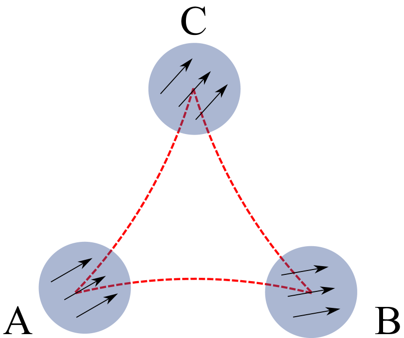
Figure 2: Three magnetized patches in a plane, forming a hyperbolic triangle. It is not possible to give a meaningful definition of the direction of magnetization, since parallel-transport of a vector from A to B and A to C, will not result in vectors that will match upon parallel-transport from B to C or vice versa.

The direction of the order-parameter at $A$ may be parallel-transported to $B$ and $C$ along the geodesics $\overline{AB}$ and $\overline{AC}$, respectively. If now we continue the parallel-transport from $B$ to $C$ along $\overline{BC}$, the two transported magnetization directions will not match. Instead, there will be an angular defect $\theta$ between the two magnetizations that is proportional to the enclosed area $\mathcal{A}$ of the hyperbolic triangle:

$$\theta=\mathcal{A}\kappa^{2}$$ (9)

This formula follows from the fact that the vectors are parallel-transported such that the angle between the geodesic curve and the vector is a constant. Since hyperbolic triangles have angles which sum to $\pi-\mathcal{A}\kappa^{2}$ (coxeter1969introduction ), we are left with the angular defect stated in (9). Thus the ordered state in hyperbolic space will in general be more complicated. Inside the radius of curvature, where $\mathcal{A}<1/\kappa^{2}$, a uniform direction may be meaningfully defined.
In order to determine the nature of the ordered state, we study the symmetry-broken state of the action $S$ at the lowest order in a $1/N$ expansion, i.e. we peform a saddle point analysis of the partition function

$$Z=\int D\bm{\phi}\exp(-S),$$ (10)

and then include higher-order fluctuations in a systematic fashion. Here, the action $S$ is given by:

$$S=\beta\int dV\ \frac{1}{2}\left[\bm{\phi}\left(\mu_{0}-\nabla^{2}\right)\bm{\phi}+\frac{u}{2N}\left(\bm{\phi}\cdot\bm{\phi}\right)^{2}\right].$$ (11)

We rewrite this by performing a Hubbard-Stratonovich decoupling of the $(\bm{\phi}\cdot\bm{\phi})^{2}$ term, whereupon the action becomes

$$S=\frac{\beta}{2}\int dV\left[\bm{\phi}\left(\mu_{0}+i\lambda(\bm{x})-\nabla^{2}\right)\bm{\phi}+\frac{N}{2u}\lambda^{2}(\bm{x})\right].$$

Now we integrate out all $\phi_{i}$ with the exception of the one component, along which the spins near a chosen point order and which we will label $\sigma(\bm{x})$. Moreover, we introduce a source field $h(\bm{x})$ for $\sigma(\bm{x})$. This leads to the action

$$S = \beta\int dV\ \frac{1}{2}\left[\sigma(\bm{x})\left(\mu_{0}+i\lambda(\bm{x})-\nabla^{2}\right)\sigma(\bm{x})+\frac{N}{2u}\lambda^{2}(\bm{x})\right]$$

$$+\frac{N-1}{2}\mathrm{Tr}\left[\log(\mu_{0}+i\lambda(\bm{x})-\nabla^{2})\right]$$

$$-\beta\int dV\ h(\bm{x})\sigma(\bm{x})$$

for the partition function $Z=\int D\sigma D\lambda\exp(-S)$.
The saddle point solutions are determined by the conditions $\frac{\delta S}{\delta\sigma(\bm{x})}=0$ and $\frac{\delta S}{\delta\lambda(\bm{x})}=0$, which result in the two equations

$$\left(\mu(\bm{x})-\nabla^{2}\right)\sigma(\bm{x}) = h(\bm{x})$$ (12)

$$\mu(\bm{x})-\mu_{0} = uT\langle\bm{x}|\frac{1}{\mu(\bm{x})-\nabla^{2}}|\bm{x}\rangle$$ (13)

$$+\frac{u}{N}\sigma^{2}(\bm{x})$$

with $\mu(\bm{x})=\mu_{0}+i\lambda(\bm{x})$.
We will use these equations to work out the critical exponents including higher-order corrections in section IV. Here, we will only analyze equation (12) to find the susceptibility $\chi(\bm{x},\bm{x}^{\prime})=\delta\sigma(\bm{x})/\delta h(\bm{x}^{\prime})|_{h(\bm{x}^{\prime})=0}$, which, by virtue of (12), satisfies

$$\left(\mu(\bm{x})-\nabla^{2}\right)\chi(\bm{x},\bm{x}^{\prime}) = \delta(\bm{x}-\bm{x^{\prime}}).$$ (14)

As we approach the phase transition from high temperatures, $\mu(\bm{x})$ may be assumed to be homogeneous. Using the formalism of the next section, this equation may be transformed into momentum space whereupon it becomes

$$\chi_{p}=\frac{1}{\mu+\kappa^{2}+p^{2}},$$ (15)

where $p\geq 0$ are the eigenvalues of the Laplacian. Note the presence of the ‘mass term’ $\kappa^{2}$ in the denominator. This is a consequence of the fact that the Laplace operator in hyperbolic space has a gapped eigenvalue spectrum, as will be seen below. A criterion for the presence of the phase transition is the condition that $\chi_{p}$ diverge. The highest value of $\mu$ when this happens is $\mu=-\kappa^{2}$, where the $p=0$ mode of the susceptibility diverges. Thus the phase transition takes place at $\mu=-\kappa^{2}$ with an order that is determined by the $p=0$ Fourier mode. In contrast to flat space, the $p=0$ eigenmode of the Laplace operator cannot be one of homogeneous order, in agreement with the foregoing argument about angular defects. Instead, it corresponds to a diminishing of the magnetization $\sigma$ along the one direction, that we chose not to integrate out. In other words, due to the lack of a global direction of magnetization, focussing on one component of the $N$-component vector, entails that one is eventually considering projections of the magnetization vector instead of the full vector. The diminishing of this projection takes place according to the formula

$$\sigma(r)=\sigma_{0}\frac{\kappa r}{\sinh\kappa r},$$ (16)

where $r$ is the geodesic distance from the origin, where the unintegrated component and local magnetization direction coincide and $\sigma_{0}$ is the magnitude of the magnetization at the origin. The phase transition corresponds to the formation of infinitely many patches, more precisely three-dimensional regions, of characteristic sizes $1/\kappa$, which have nearly uniform magnetization. The decay of $\sigma(r)$ in Eq. (16) does not imply a decay of the magnitude of the order parameter, but must be interpreted as the order parameter rotating away from the chosen direction of the vector ${\bm{\phi}}$.

IV Momentum space representation

We come now to the technical part of this paper that will allow us to analyze the saddle point equations (12), (13) and compute critical exponents. In order to make progress with the calculations, it is convenient to obtain the momentum space representation of functions that are translationally invariant in hyperbolic space. Let $\psi(d_{PQ})$ be a given function of the geodesic distance between two points $P$ and $Q$. The functional dependence on the two points will not have an arbitrary form, but will rather be expressed through the geodesic distance $d_{PQ}$ between these two points. This distance is the length of the geodesic curve connecting these points. Explicit computation of this length yields the formula

$$\cosh{\kappa d_{PQ}} = \cosh{\kappa r}\cosh{\kappa r^{\prime}}-\sinh{\kappa r}\sinh{\kappa r^{\prime}}\cos{\gamma}$$

$$\cos{\gamma} = \cos{\theta}\cos{\theta^{\prime}}+\sin{\theta}\sin{\theta^{\prime}}\cos{(\phi-\phi^{\prime})}.$$ (17)

The fact that such a function $\psi$ depends on the six coordinates not in an arbitrary way, but only through the geodesic distance, allows us to expand $\psi(d_{PQ})$ in terms of the eigenstates of the Laplace operator in hyperbolic space. Since hyperbolic space may be defined as the set of all points equidistant from the origin in Minkowski space, this Laplace operator is identical to the one obtained by writing down the 4-dimensional Laplace operator in angular coordinates and restricting the distance from the origin to a constant. A similar situation was considered by Fock Fock:1935kq , who studied the problem on a 3-sphere embedded in 4-dimensional euclidean space. The eigenfunctions of the Laplacian on this 3-sphere are the generalized spherical harmonics of three angles. Their full description was given in Fock:1935kq . We find the eigenfunctions of the Laplacian in hyperbolic space by multiplying one of the angles in Fock’s solution by the imaginary unit, a prescription sketched briefly in an appendix of lifshitz1963investigations .
The hyperbolic Laplacian is given by

$$\Delta = \frac{1}{\sinh^{2}\kappa r}\partial_{r}(\sinh^{2}\kappa r\partial_{r}\psi)+\frac{\kappa^{2}}{\sinh^{2}(\kappa r)}\Delta_{S^{2}}$$

$$\Delta_{S^{2}} = \frac{1}{\sin\theta}\partial_{\theta}\left(\sin\partial_{\theta}\psi\right)+\frac{1}{\sin^{2}\theta}\partial_{\phi}^{2}\psi.$$ (18)

The eigenfunctions are then given by

$$\psi_{qlm}(r,\theta,\phi)=\Pi_{ql}(\kappa r)Y_{lm}(\theta,\phi)$$ (19)

with eigenvalues

$$\Delta\psi_{qlm}(r,\theta,\phi)=-(\kappa^{2}+q^{2})\psi_{qlm}(r,\theta,\phi).$$ (20)

Here the $Y_{lm}$ are the ordinary spherical harmonics on the 2-sphere and the $\Pi_{pl}$ are special functions that solve the radial part of the eigenvalue equation

$$\frac{d^{2}}{dr^{2}}\Pi_{ql}+2\kappa\coth{\kappa r}\frac{d}{dr}\Pi_{ql}-\frac{l(l+1)\kappa^{2}}{\sinh^{2}{\kappa r}}\Pi_{ql}(\kappa r)=-(\kappa^{2}+q^{2})\Pi_{ql}(\kappa r).$$ (21)

The solutions can be expressed in a Rayleigh-type formula

$$\Pi_{pl}(x)=\frac{\sinh^{l}x}{M_{l}}\left(\frac{d^{l+1}}{d(\cosh x){}^{l+1}}\right)\cos(px)$$ (22)

where

$$M_{l}^{2}=\left(\frac{q}{\kappa}\right)^{2}\left[\left(\frac{q}{\kappa}\right)^{2}+1^{2}\right]\dots\left[\left(\frac{q}{\kappa}\right)^{2}+l^{2}\right]$$ (23)

is a normalization constant. The differential equation being of the Sturm-Liouville form, these functions satisfy the orthogonality relation

$$\int\limits_{0}^{\infty}dr\sinh^{2}{(\kappa r)}\ \Pi_{ql}(\kappa r)\Pi_{q^{\prime}l}(\kappa r)=\frac{\pi}{2}\delta(q-q^{\prime}).$$ (24)

IV.1 Addition theorem

The eigenstates $\psi_{plm}(r,\theta,\phi)$ satisfy an addition theorem, which was derived for the 3-sphere by Fock Fock:1935kq . In the latter case of the 3-sphere this formula is fully analogous to the addition theorem for two-dimensional spherical harmonics. Again, by multiplying one of the angles by the imaginary unit, we obtain the corresponding addition theorem valid in hyperbolic space

$$\frac{\sin(qd)}{\sinh(\kappa d)}=\frac{\kappa}{q}\sum_{l=0}^{\infty}(2l+1)\Pi_{ql}(\kappa r)\Pi_{ql}(\kappa r^{\prime})P_{l}(\cos\gamma),$$ (25)

where the $P_{l}(\cos\gamma)$ are the Legendre polynomials in $\cos\gamma$.
As a demonstration of the use of this formula, let us derive the magnetization texture of the $p=0$ eigenmode given in (16). The eigenbasis expansion of $\chi$ reads

$$\chi(\bm{r},\bm{r}^{\prime})=\int dp\sum_{l}(2l+1)\chi_{p}\Pi_{pl}(\kappa r)\Pi_{pl}(\kappa r^{\prime})P_{l}(\cos\gamma).$$ (26)

Insertion of $\chi_{p}$ from (15) into this equation at the critical point $\mu=-\kappa^{2}$, yields the real-space form of $\chi$. Now we construct the real-space form of only the $p=0$ mode, which gives

$$\sigma(d(\bm{r},\bm{r}^{\prime})) = \lim_{p\rightarrow 0}\sum_{l}(2l+1)\frac{\sigma_{p}}{p^{2}}\Pi_{pl}(\kappa r)\Pi_{pl}(\kappa r^{\prime})P_{l}(\cos\gamma)$$ (27)

$$= \sigma_{0}\frac{\kappa d(\bm{r},\bm{r}^{\prime})}{\sinh\kappa d(\bm{r},\bm{r}^{\prime})},$$

as claimed.

IV.2 Extraction of coefficients and inversion formula

The identity (25) will be crucial in obtaining the expansion coefficients of a given function $\psi(d)$ of the geodesic distance. This distance being a non-negative quantity, the value of $\psi$ for negative arguments is irrelevant. In particular we may redefine $\psi$ for negative arguments such that it becomes an even function. This allows us to Fourier expand $\psi$ as follows

$$\psi(d)\sinh\kappa d = \frac{\kappa}{2\pi^{2}}\int\limits_{-\infty}^{+\infty}dp\ \psi_{p}p\sin({pd}),$$ (28)

where we have chosen to split off a factor of $\kappa p/(2\pi^{2})$ in the definition of the expansion coefficient for later convenience. Inserting (25) we obtain

$$\psi(d)=\frac{\kappa}{2\pi^{2}\sinh\kappa d}\int\limits_{-\infty}^{+\infty}dp\ \psi_{p}p\sin({pd})=\frac{\kappa^{2}}{2\pi^{2}}\int\limits_{-\infty}^{+\infty}dp\sum_{l=0}^{\infty}(2l+1)\psi_{p}\Pi_{pl}(\kappa r)\Pi_{pl}(\kappa r^{\prime})P_{l}(\cos\gamma)$$ (29)

and have thereby managed to expand the arbitrary function $\psi$ in the new basis with coefficients

$$\psi_{p}=\frac{\pi i}{\kappa p}\int\limits_{-\infty}^{+\infty}dx\psi(|x|)\sinh(\kappa x)e^{-ipx}.$$ (30)

Let us briefly comment on the structure of the expansion. Note that in (29) the expansion coefficient $\psi_{p}$ has no dependence on $l$. In fact, the statement of (29) is that any function that depends on the set of coordinates $(r,\theta,\phi),(r^{\prime},\theta^{\prime},\phi^{\prime})$ only through the geodesic distance of the two points, can have no explicit $l$ or $m$ dependence of $\psi_{p}$.
Conversely, to find the real-space function $\psi(d)$ from the knowledge of the coefficients $\psi_{p}$ in the expansion (29) we use (28) which results in the inversion formula

$$\psi(d)=\frac{\kappa}{2\pi^{2}i\sinh\kappa d}\int\limits_{-\infty}^{+\infty}dp\ \psi_{p}pe^{ipd}.$$ (31)

IV.3 Convolution theorem

Let $f$ and $g$ be two-point functions that depend on the geodesic distances $d_{PQ}$ and $d_{QR}$, respectively. When we multiply these functions and integrate $Q$ over all of hyperbolic space, the resulting function $h$ can only depend on the geodesic distance between points $P$ and $R$. This convolution will in general be difficult to carry out in real-space. The fact that the $\Pi_{plm}$ and the $Y_{lm}$ are orthogonal functions, however, allows us to reduce the convolution of $f$ and $g$ to a multiplication in momentum-space. This is seen explicitly by rewriting the relation

$$\int dV_{Q}f(d_{PQ})g(d_{QR})=h(d_{PR})$$ (32)

in the momentum representation (29) with expansion coefficients $f_{p},g_{p},h_{p}$ and using the orthogonality relations for the radial functions and the spherical harmonics. Then this convolution formula translates into

$$f_{p}g_{p}=h_{p}.$$ (33)

The solution of the Dyson equation below will require knowledge about the momentum-space representation of the Dirac $\delta$-function in hyperbolic space, which we denote by either $\delta_{PQ}$ or $\delta(\bm{r},\bm{r}^{\prime})$. We define this function by the condition that convolution of an arbitrary function $\psi(d_{PQ})$ with $\delta(d_{QR})$ must yield $\psi(d_{PR})$. Translating this condition into momentum space, we immediately read off from (33) the relation $\delta_{p}=1$ and obtain thereby

$$\delta_{PQ} = \frac{\kappa^{2}}{2\pi^{2}}\int\limits_{-\infty}^{+\infty}dp\sum_{l=0}^{\infty}(2l+1)$$ (34)

$$\times\Pi_{pl}(\kappa r)\Pi_{pl}(\kappa r^{\prime})P_{l}(\cos\gamma).$$

Conversely, however, the multiplication of two functions in real-space does not translate into a simple convolution integral in momentum-space, but rather a double-integral. Given the product

$$f(d_{PQ})g(d_{PQ})=h(d_{PQ})$$ (35)

the corresponding momentum-space equation is found by employing the representation (31)

$$h_{k}=\frac{1}{4\pi^{2}k}\int\limits_{-\infty}^{\infty}dp\int\limits_{-\infty}^{\infty}dqf_{p}g_{q}pq\tanh\left[\frac{p+q-k}{2\kappa}\pi\right]$$ (36)

i.e. instead of a single integral a double integral with kernel is obtained.
In the limit $k\rightarrow 0$ the symmetry properties of $f_{p}$ and $g_{q}$ may be used to rewrite this kernel as

$$\lim_{k\rightarrow 0}h_{k}=\frac{1}{8\pi\kappa}\int\limits_{-\infty}^{\infty}dp\int\limits_{-\infty}^{\infty}dq\ \frac{pqf_{p}g_{q}}{\cosh^{2}\frac{\pi(p-q)}{2\kappa}}.$$ (37)

This formula will be used in section VI in evaluating the corrections to the critical exponent $\gamma$.

V Critical exponents

The previous formalism may now be employed to analyze the saddle point equations (12) and (13). These equations describe the physics of the model at lowest order in $1/N$. Given this fact, all exponents that we derive below represent the lowest order contribution in $1/N$. In principle these are only the lowest order terms in an expansion of the critical exponents in a power series in $1/N$. In flat three-dimensional space there are indeed further corrections. The main result of this paper, derived in section VI, is to establish the absence of such corrections for $\eta$ and $\gamma$ in three-dimensional hyperbolic space.
We begin by computing the bare Green’s function $G^{(0)}(p)$ in momentum space for constant $\mu$ in the action for $\sigma(\bm{x})$. The real-space definition of the bare $G^{(0)}(\bm{r})$ is obtained by inverting the action, i.e.

$$\left(\mu-\nabla^{2}\right)G^{(0)}(\bm{r},\bm{r}^{\prime})=\delta(\bm{r},\bm{r}^{\prime}).$$ (38)

Inserting

$$G^{(0)}(\bm{r},\bm{r}^{\prime}) = \frac{\kappa^{2}}{2\pi^{2}}\int\limits_{-\infty}^{\infty}dp\sum_{l}(2l+1)$$ (39)

$$\times G^{(0)}(p)\Pi_{pl}(\kappa r)\Pi_{pl}(\kappa r^{\prime})P_{l}(\cos\gamma)$$

and the representation of $\delta(\bm{r},\bm{r}^{\prime})$ in (34), it is found that

$$G^{(0)}(p)=\frac{1}{(\mu+\kappa^{2}+p^{2})}.$$ (40)

At the critical point, $\mu=-\kappa^{2}$, we have a power-law dependence on $p$. Employing the inversion formula, we find the real-space dependence

$$G^{(0)}(\bm{r},\bm{r}^{\prime}) = \frac{\kappa}{2\pi^{2}i\sinh\kappa d}\int\limits_{-\infty}^{\infty}dp\frac{pe^{ipd}}{(\mu+\kappa^{2}+p^{2})}$$ (41)

$$= \frac{\kappa}{2\pi}\frac{e^{-\sqrt{\mu+\kappa^{2}}d}}{\sinh\kappa d},$$

where $d$ is the geodesic distance between $\bm{r}$ and $\bm{r}^{\prime}$. Evidently, even at the critical point the Green’s function decays exponentially, in accord with the previous remarks about parallel-transport.

	$\eta$	$\gamma$
$\kappa=0$	$\frac{8}{3\pi^{2}}\frac{1}{N}+\mathrm{O}\left(\frac{1}{N^{2}}\right)$	$2-\frac{24}{\pi^{2}}\frac{1}{N}+\mathrm{O}\left(\frac{1}{N^{2}}\right)$
$\kappa\neq 0$	$0$	$2$

Table 1: Critical exponents in flat and hyperbolic space.

V.1 Critical Exponent $\eta$

Let us now proceed to the evaluation of the exponent $\eta$. At the critical point $\mu=-\kappa^{2}$ the power-law form of the curved-space bare Green’s function in (40) agrees with the flat-space limit. The exponent $\eta$ may therefore be defined through the relation

$$G(p)\propto\frac{\Lambda^{-\eta}}{p^{2-\eta}}.$$ (42)

We see that the bare $G^{(0)}(p)$, i.e. the lowest order form of the Green’s function in an $1/N$ expansion, has $\eta=0$.

V.2 Critical Exponents $\nu$ and $\gamma$

We now study the behavior of the correlation-length as the critical temperature is approached from the disordered regime by examining the saddle point equation (13). In the regime $\mu>-\kappa^{2}$, the magnetization will be zero. We may therefore set $\sigma=0$ and obtain

$$\mu = \mu_{0}+\frac{uT}{2\pi^{2}}\int\limits_{0}^{\Lambda}dq\frac{q^{2}}{\mu+\kappa^{2}+q^{2}}$$ (43)

$$= \mu_{0}+\frac{uT}{2\pi^{2}}\Lambda-\frac{uT}{2\pi^{2}}\sqrt{\mu+\kappa^{2}}\pi.$$

At $T=T_{c}$, where $\mu=-\kappa^{2}$, we have

$$-\kappa^{2}=\mu_{0}+\frac{uT_{c}}{2\pi^{2}}\Lambda,$$ (44)

which allows us to remove $\mu_{0}$ from (43). Now close to $\mu\gtrsim-\kappa^{2}$, the quantity $\sqrt{\mu+\kappa^{2}}$ dominates over $\mu+\kappa^{2}$. Thus we neglect the latter and find

$$\sqrt{\mu+\kappa^{2}} = \frac{1}{\pi}\frac{T-T_{c}}{T_{c}}\Lambda.$$ (45)

The length $\xi$ that diverges at the critical point is defined by

$$\xi=\frac{1}{\sqrt{\mu+\kappa^{2}}},$$ (46)

which is the natural length scale of the problem as follows from the correlation function Eq.(40) in its eigenbasis. At the same time, the real-space form of the correlation function in Eq.(41) shows that $G^{(0)}(d)$ decays exponentially beyond the curvature $1/\kappa$, even for $\xi^{-1}=0$ . However, what matters is the eigenbasis of the correlation function, where $G$ becomes scale invariant at $T_{c}$. The decay of the correlation function in real-space will, however, have impact on the $1/N$ corrections of the critical exponents. Defining a critical exponent $\nu$ through ${\xi}$, we find from (45) and (46) the exponent

$$\xi\sim(T-T_{c})^{-1}\rightarrow\nu=1.$$ (47)

According to (15) the zero-momentum susceptibility is

$$\chi_{q=0}=\frac{1}{\mu+\kappa^{2}}$$ (48)

and by using (45) we find $\gamma=2$.
We emphasize here explicitly the fact that both exponents are not mean-field exponents. The latter are given by $\nu_{\text{MF}}=\frac{1}{2}$ and $\gamma_{\text{MF}}=1$.

VI Corrections to critical exponents

Corrections to the critical exponents $\eta$ and $\gamma$ are found by inspecting the self-energy. In flat space this calculation is described in PhysRevA.7.2172 and we find that the general procedure carries over to hyperbolic space. This procedure consists in first determining how a correction to a critical exponent would manifest itself in the self-energy and calculating the order $O(1/N)$ diagrams to see if such contributions are present.
We start with the action (11). The Dyson equation in real-space reads

$$G(\bm{r}_{P},\bm{r}_{R})=G^{(0)}(\bm{r}_{P},\bm{r}_{R})+\int d\bm{r}_{Q}\int d\bm{r}_{Q^{\prime}}\ G^{(0)}(\bm{r}_{P},\bm{r}_{Q})\Sigma(\bm{r}_{Q},\bm{r}_{Q^{\prime}})G(\bm{r}_{Q^{\prime}},\bm{r}_{R})$$ (49)

and is converted to

$$G^{-1}(p)=G^{(0)-1}(p)+\Sigma(p)$$ (50)

by application of the convolution theorem. We follow PhysRevA.7.2172 in rewriting this equation as

$$G^{-1}(p)=\left(G^{(0)-1}(p)+\Sigma(0)\right)+\Sigma(p)-\Sigma(0)$$ (51)

and redefining the new inverse bare Green’s function $G^{0-1}(p)$ to be the first term, i.e.

$$G^{0-1}(p)=\mu_{0}+\Sigma(0)+\kappa^{2}+p^{2}=\mu+\kappa^{2}+p^{2}.$$ (52)

This has the advantage that at $T=T_{c}$ the ‘mass’ $\mu+\kappa^{2}$ of the bare propagator vanishes. As a consequence of this redefinition, self-energy insertions in diagrams now take the form $\Sigma(p)-\Sigma(0)$ instead of $\Sigma(p)$.
The large-$N$ structure of the model allows us to restrict ourselves to a small number of diagrams. The calculated corrections will be exact to order $1/N$. The coupling constant $u$ in the action is multiplied by a factor $1/N$. Due to the presence of $N$ fields, there is a summation over the field index at every $(\phi\cdot\phi)^{2}$ interaction vertex. We represent this interaction term by a dashed line. On the other hand, a summation over the field index at every vertex produces a factor $N$. Thus the series of bubbles connected by $-u/N$ interaction lines, as shown in Figure 3, are all of order $1/N$ and need to be included for consistency. We denote this sum by a wiggly line and use the symbol $D(p)$. It satisfies the relation

$$D(p)=-\frac{u/N}{1+\frac{u}{2}\Pi(p)}\approx-\frac{2}{N\Pi(p)}$$ (53)

where $\Pi(p)$ is the polarization operator. The approximation comes from the large-$u$ limit, which we will be considering from here on. In real-space $\Pi$ is given by

$$\Pi(\bm{r},\bm{r}^{\prime})=G^{0}(\bm{r},\bm{r}^{\prime})^{2}=\frac{\kappa^{2}}{4\pi^{2}}\frac{e^{-2\sqrt{\mu+\kappa^{2}}d}}{\sinh^{2}\kappa d},$$ (54)

where $d$ is the geodesic distance between $\bm{r}$ and $\bm{r}^{\prime}$. Using (30) we find

$$\Pi_{p}(\mu)=-\frac{1}{2\pi p}\mathrm{Im}\left[\psi\left(\frac{1}{2}-\frac{ip}{2\kappa}+\frac{\sqrt{\mu+\kappa^{2}}}{\kappa}\right)\right],$$ (55)

where $\psi(z)\equiv\frac{d}{dz}\log{\Gamma(z)}$ is the digamma function. With (53) we find

$$D_{p}(\mu)=\frac{2\pi p}{N}\frac{1}{\mathrm{Im}\left[\psi\left(\frac{1}{2}-\frac{ip}{2\kappa}+\frac{\sqrt{\mu+\kappa^{2}}}{\kappa}\right)\right]}.$$ (56)

Figure 3: Dyson equation for the screened interaction $D(p)$

Figure 4: Relevant $O(1/N)$ diagrams. In flat space, diagram (a) contributes to $\eta$ and diagram (b) to $\gamma$.

We present the calculation of the correction to $\eta$ in detail. The calculation of the correction to $\gamma$ is much more tedious and is only sketched. The result in both cases is the absence of any corrections due to the regularizing character of finite curvature.

VI.1 Order $\mathcal{O}(1/N)$ correction of $\eta$

As we have seen $\eta=0$ at lowest order in $1/N$. We now determine the $1/N$ correction to this result. We have defined $\eta$ in (42). Such a correction would manifest itself in the self-energy. For large-$N$ this critical exponent can be expanded and reads

$$G(p)=\frac{\kappa}{4\pi}\frac{\Lambda^{-\eta}}{p^{2-\eta}}=\frac{\kappa}{4\pi}\frac{\Lambda^{-\eta}}{p^{2}-\eta\ p^{2}\log p},$$ (57)

i.e. a correction would lead to a $p^{2}\log p$ term in the self-energy and could be found as the coefficient of such a term. In flat space there is indeed such a correction. We will now show that this $p^{2}\log p$ term of flat space is regularized in hyperbolic space. The polarization operator (55) at the critical point $\mu=-\kappa^{2}$ becomes

$$\Pi(p)=\frac{1}{4p}\tanh\left(\frac{\pi}{2\kappa}p\right).$$ (58)

In flat-space the $p^{2}\log p$ contribution is produced by the diagram in Figure 4a. To write down this term we take the real-space form of $D(p)$, which is obtained from (53) with (30)

$$D(d_{PQ}) = \frac{8\kappa^{4}\cosh(\kappa d_{PQ})}{N\pi^{2}\sinh^{4}(\kappa d_{PQ})}.$$ (59)

The self-energy in real-space is obtained by multiplying $D$ with the bare Green’s function

$$\Sigma(d_{PQ}) = D(d_{PQ})G^{(0)}(d_{PQ})$$ (60)

$$= \frac{8\kappa^{5}}{N\pi^{3}}\frac{\cosh(\kappa d_{PQ})}{\sinh^{5}(\kappa d_{PQ})}.$$ (61)

Using again formula (30), we can write this in momentum space as

$$\Sigma(p) = \frac{8(\kappa^{2}+p^{2})}{3N\pi^{2}}\times$$

$$\left[\text{Re}\psi\left(-\frac{3}{2}+i\frac{p}{2\kappa}\right)+\frac{2/3\ p^{2}}{9\kappa^{2}+p^{2}}+\gamma-\frac{5}{2}\right],$$

where $\gamma$ is the Euler-Mascheroni constant. Taking the flat-space limit $\kappa\rightarrow 0$ with fixed $p$, we obtain the asymptotic relation

$$\Sigma(p)\sim\frac{8}{3\pi^{2}N}p^{2}\left(\log\frac{p}{2\kappa}+\gamma-\frac{11}{6}\right).$$ (63)

The appearance of $\kappa$ in this formula is owed to the fact that we measure all momenta in units of $\kappa$.
In the opposite regime, where $p$ tends to $0$ for fixed curvature, we have instead of a logarithmic divergence the finite value

$$\Sigma(p)\sim\frac{8\kappa^{2}}{3\pi^{2}N}\left(\frac{17}{6}-4\log 2-\gamma\right).$$ (64)

This regularizing behavior of the finite curvature is shown in Figure 5, where we defined a quantity $\eta(p)\equiv\frac{d}{d\log p}\left[\frac{\Sigma(p)-\Sigma(0)}{p^{2}}\right]$, which in flat space would yield a finite $\eta$. In hyperbolic space at sufficiently small $p$, i.e. long length-scales, the log behavior of the self-energy (VI.1) is cut off and $\eta(p)$ is suppressed to $0$.

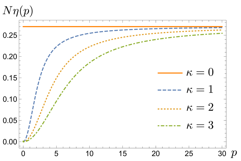
Figure 5: Here we have defined a function $\eta(p)\equiv\frac{d}{d\log p}\left[\frac{\Sigma(p)-\Sigma(0)}{p^{2}}\right]$. In flat space $\eta(p)=\frac{8}{3\pi^{2}N}$, whereas in hyperbolic space it is always regularized by curvature and tends to $0$ at long length-scales.

VI.2 Order $\mathcal{O}(1/N)$ correction of $\gamma$

The exponent $\gamma$ is found from the divergence of the susceptibility at $p=0$. We find at zero-momentum for the full Green’s function

$$G^{-1}\left({\mu(T)}\right) = \mu_{0}(T)+\kappa^{2}+\Sigma\left(\mu(T)\right)$$ (65)

$$= \mu(T)+\kappa^{2}.$$

In the following all calculations will be for zero external momenta, thus we have suppressed the momentum arguments. Subtracting from this equation the same equation evaluated at $T=T_{c}$, we find

$$\mu(T)+\kappa^{2}-\Sigma\left(\mu(T)\right)+\Sigma\left(0\right)=\mu_{0}(T-T_{c}).$$ (66)

We have found $\gamma=2$ at lowest order in section V.2. Writing $1/\gamma=1/2-\Delta$ and using the definition of the exponent via $\mu_{0}(T-T_{c})\sim\left(\mu(T)+\kappa^{2}\right)^{1/\gamma}$ for $T$ near $T_{c}$, we obtain

$$-\Sigma\left(\mu(T)\right)+\Sigma\left(0\right) \sim \sqrt{\mu(T)+\kappa^{2}}$$

$$-\Delta\sqrt{\mu(T)+\kappa^{2}}\log\left({\mu(T)+\kappa^{2}}\right)$$

valid near $T\gtrsim T_{c}$. The first term on the right-hand side is an $O(1)$ term and was already obtained in section V. It is produced by a diagram, which is obtained from diagram 4b by removing the internal wiggly line.
There are two $O(1/N)$ diagrams that have to be considered in computing the correction $\Delta$, shown in Figures 4a and 4b. In flat space it can be shown that the diagram in Figure 4a only gives a $\sim\mu\log\mu$ correction, whereas the diagram in Figure 4b in fact yields a finite $\Delta$. We shall see now that in hyperbolic space neither diagram yields a contribution to $\Delta$, as both logarithmic divergences are regularized by $\kappa$.

VI.2.1 Diagram (a)

We begin with the diagram in Figure 4a. We denote this self-energy part by $\Sigma_{a}(\mu)$. Using eq. (37) we find

$$\Sigma_{a}(\mu)-\Sigma_{a}(0)=\frac{1}{8\pi\kappa}\int\limits_{-\Lambda}^{\Lambda}dq\int\limits_{-\Lambda}^{\Lambda}dp\left[G_{p}(\mu)D_{q}(\mu)-G_{p}(0)D_{q}(0)\right]\frac{pq}{\cosh^{2}\left(\frac{\pi}{2\kappa}(p-q)\right)}.$$ (68)

The hyperbolic cosine effectively cuts off contributions with $|p-q|\gg\kappa$. Hence the $q$-integral may be approximated by limiting the integration to this region. Insertion of $G_{p}(\mu)$ and $D_{q}(\mu)$ from (40) and (56) and subsequent expansion in $\mu$ results in a large number of elementary integrals. All logarithmic terms stemming from these integrals are of the form $\log(c\kappa^{2}+\mu)$, where $c$ is either $1$ or $4$. In other words, for finite $\kappa$ no terms proportional to $\log\mu$ are present.

VI.2.2 Diagram (b)

Similarly the $\sqrt{\mu}\log\mu$ divergence of the diagram 4b in flat-space is regularized. The self-energy expression corresponding to this diagram is obtained by noticing that diagram 4b is the result of attaching to the self-energy in 4a two legs of the interaction vertex. It is correspondingly given by

$$\Sigma_{b}(\mu) = \frac{1}{8\pi\kappa}\int dq\int dq^{\prime}\ qq^{\prime}\ G_{q}(\mu)^{2}\left[\Sigma_{a}(q^{\prime},\mu)-\Sigma_{a}(0,\mu)\right]\frac{1}{\cosh^{2}{\frac{\pi(q-q^{\prime})}{2\kappa}}}$$ (69)

$$\approx \frac{\kappa^{2}}{2\pi^{2}}\int dq^{\prime}\ \frac{q^{\prime 2}}{[(q^{\prime}-2\kappa/\pi)^{2}+\mu+\kappa^{2}][(q^{\prime}+2\kappa/\pi)^{2}+\mu+\kappa^{2}]}\left[\Sigma_{a}(q^{\prime},\mu)-\Sigma_{a}(0,\mu)\right]$$

where the same approximation as before has been made. In the integrand the momentum-dependent self-energy $\Sigma_{a}(q,\mu)$ is required. According to (36) this is given by

$$\Sigma_{a}(q^{\prime},\mu)=\frac{1}{4\pi^{2}q^{\prime}\kappa}\int\limits_{-\Lambda}^{\Lambda}dp^{\prime}\int\limits_{-\Lambda}^{\Lambda}dp\left[G_{p}(\mu)D_{p}^{\prime}(\mu)-G_{p}(0)D_{p}^{\prime}(0)\right]pp^{\prime}\tanh\left(\frac{p+p^{\prime}-q^{\prime}}{2\kappa}\pi\right).$$ (70)

Inside the $p$-integral we approximate the $\tanh$-function in the region $|p+p^{\prime}-q|<\frac{2\kappa}{\pi}$ by its argument and outside this region by the sign-function. Then the $p$-integral may be carried out without a cutoff and we are left with a $p^{\prime}$-integral. Insertion of (70) into (69) and integration over $q^{\prime}$ results in

$$\Sigma_{b}(\mu)=\frac{2\pi^{2}}{\kappa\lambda}\int\limits_{0}^{\Lambda}dq^{\prime}\frac{q^{\prime 2}}{\mathrm{Im}\psi\left(\frac{1}{2}-\frac{iq^{\prime}}{2\kappa}+\frac{\lambda}{\kappa}\right)}\log\frac{(q^{\prime}-2\kappa)^{2}+4\lambda^{2}}{(q^{\prime}+2\kappa)^{2}+4\lambda^{2}}+R(\kappa).$$ (71)

where $R(\kappa)$ denotes terms that tend to $0$ with $\kappa\rightarrow 0$. The first term on the right-hand side reproduces for $\kappa=0$ fully the flat space formula for $\Sigma_{b}$. This self-energy contains the $\sqrt{\mu}\log\mu$ term. For finite $\kappa$, however, the integral in (71) is fully regularized and a $\sqrt{\mu}\log\mu$ term is avoided. Thus, we conclude that no singular correction to the $\mu$ dependence of the self-energy emerges, i.e. the exponent $\gamma$ is also unchanged compared to the leading order $1/N$ expression given above.

VII Discussion

The aim of this paper was to investigate critical phenomena in hyperbolic space. Our key finding is that for a $\bm{\phi}^{4}$-model embedded in hyperbolic space a new fixed point emerges at finite curvature $\kappa$. If $\kappa>0$ the critical exponents are governed by the strong curvature limit. Interestingly, these exponents are given by leading order terms of the $1/N$ expansion. Thus, while the numerical values of the exponents are now simpler, they continue to obey hyperscaling below the upper critical dimension. The physical state in the symmetry-broken regime is characterized by an unusual magnetization texture. This texture consists of regions of size of the order of the radius of curvature $1/\kappa$ where the vector $\bm{\phi}$ has nearly uniform direction. Beyond this region the finite value of the curvature starts to play an important role, since a global direction in hyperbolic space is not a well-defined concept. It is therefore not possible to establish a uniform direction of the magnetization vector. In fact, as we have illustrated in Figure 2, the parallel transport of a local direction from region $A$ to $B$ and then from $B$ to $C$ is not the same as the direct parallel transport from $A$ to $C$. It is this lack of transitivity which is the origin of the resulting magnetization texture.
The fact that the $\kappa\neq 0$ values of exponents are different from the flat space $\kappa=0$ limit may be understood using standard crossover arguments as we now show using the example of magnetic susceptibility. Let $f(t,h,\kappa)$ be the singular part of the free energy density, where $t\propto(T-T_{c})/T_{c}$ measures the distance to the critical point and $h$ is the external field. Then the following scaling transformation holds

$$f(t,h,\kappa)=b^{-3}f\left(b^{1/\nu_{f}}t,b^{y_{f}}h,b\kappa\right),$$ (72)

with exponents $\nu_{f}$ for the correlation length and scaling dimension of the conjugate field $y_{f}=\beta_{f}\delta_{f}/\nu_{f}$ that refer to the flat space ($\kappa=0$) limit. The curvature is a relevant perturbation with positive scaling dimension, i.e. the infrared behavior is governed by the infinite curvature fixed point, where all scales (except of course for the inverse ultraviolet cut-off) are larger compared to the radius of curvature. Performing the second derivative with respect to the conjugate field, we obtain the scaling expression for the order parameter susceptibility:

$$\chi(t,\kappa) = b^{\gamma_{f}/\nu_{f}}\chi(b^{1/\nu_{f}}t,b\kappa)$$ (73)

$$= t^{-\gamma_{f}}\Phi\left(\frac{\kappa}{t^{\nu_{f}}}\right).$$

In the flat space limit $\kappa=0$, the scaling function behaves as $\Phi(x\rightarrow 0)\rightarrow\text{const.}$ and we recover the flat space results. On the other hand, our above analysis implies that for large argument $\Phi(x\gg 1)\propto x^{-\phi}$ holds with crossover exponent

$$\phi=\frac{\gamma-\gamma_{f}}{\nu_{f}}=\frac{24}{N\pi^{2}}.$$ (74)

Here $\gamma$ is the susceptibility exponent of the hyperbolic space obtained above. Thus, we find $\chi(t,\kappa)\propto\kappa^{-\phi}t^{-\gamma}$. The behavior $\kappa^{-\phi}$ is, at the considered order, fully consistent with the $\phi\log(\kappa)$ behavior that occured in our explicit analysis. We have calculated the critical exponents $\eta,\gamma$ and $\nu$ at lowest order in $1/N$ and found that these are identical to the exponents in flat three-dimensional space at lowest order. For $\eta$ and $\gamma$ we showed that $\textrm{O}(1/N)$ corrections are absent. As our calculations show, the reason for this absence is the fact that correlations are exponentially decaying beyond the radius of curvature even at the critical point. The lowest order values of the exponents are computed from local quantities, which are oblivious to the finite curvature, whereas the higher-order corrections are determined through integration over the whole of hyperbolic space, wherein the finite curvature serves to cut off the long-wavelength fluctuations. For this reason, we may also surmise the absence of corrections to the other critical exponents. It is moreover plausible to assume for the same reason that higher-order corrections to the exponents will also be absent in the $1/N$-expansion. Thus we conjecture that the critical exponents we found are correct to all orders in $1/N$.
An interesting question is how our results are modified for dimensions $d$ different from $3$. The Laplacian in $d\neq 3$ dimensions is still gapped. The only modification in our lowest order $1/N$ calculations of the critical exponents would be a change of the integration measure in (43), from $p^{2}$ to $p^{d-1}$, multiplied by a numerical factor. However, this leads again the same saddle point equations as in flat space. Thus we can make the stronger statement that all critical exponents in hyperbolic space are just the leading order $1/N$ exponents of flat space. In particular, we have $\nu=\frac{1}{d-2}$ and $\gamma=\frac{2}{d-2}$ for $d\leq 4$ and mean-field exponents for $d>4$. The upper critical dimension is $d=4$ even for finite $\kappa$.
In summary, we conclude that the description of many-particle systems in hyperbolic space is a promising avenue to investigate uniform frustration and non-trivial critical behavior within one theoretical approach.

- (1) J. M. Maldacena, The Large N limit of superconformal field theories and supergravity, Adv.Theor.Math.Phys. 2, 231–252 (1998).
- (2) S. S. Gubser, I. R. Klebanov, and A. M. Polyakov, Gauge theory correlators from non-critical string theory, Physics Letters B 428 (1998).
- (3) E. Witten, Anti-de Sitter space and holography, Adv.Theor.Math.Phys. 2, 253–291 (1998).
- (4) M. Kurata, R. Kikuchi, and T. Watari, A Theory of Cooperative Phenomena. III. Detailed Discussions of the Cluster Variation Method, The Journal of Chemical Physics (1953).
- (5) C. Domb, Advances in Physics 9 , 245 (1960).
- (6) M. F. Thorpe, Bethe Lattices, Excitations in Disordered Systems NATO Advanced Study Institute Series B78 , 85–107 (1982).
- (7) A. Georges, G. Kotliar, W. Krauth, and M. J. Rozenberg, Dynamical mean-field theory of strongly correlated fermion systems and the limit of infinite dimensions, Rev. Mod. Phys. 68, 13–125 (Jan 1996).
- (8) M. Eckstein, M. Kollar, K. Byczuk, and D. Vollhardt, Hopping on the Bethe lattice: Exact results for densities of states and dynamical mean-field theory, Phys. Rev. B 71, 235119 (Jun 2005).
- (9) C. Laumann, A. Scardicchio, and S. L. Sondhi, Cavity method for quantum spin glasses on the Bethe lattice, Phys. Rev. B 78, 134424 (Oct 2008).
- (10) G. Semerjian, M. Tarzia, and F. Zamponi, Exact solution of the Bose-Hubbard model on the Bethe lattice, Phys. Rev. B 80, 014524 (Jul 2009).
- (11) R. Mosseri and J. Sadoc, The Bethe lattice: a regular tiling of the hyperbolic plane, Journal de Physique Lettres 43(8), 249–252 (1982).
- (12) Curved Spaces - Software to visualize curved spaces, developed by Jeff Weeks. http://www.geometrygames.org/CurvedSpaces/.
- (13) G. Tarjus, S. A. Kivelson, Z. Nussinov, and P. Viot, The frustration-based approach of supercooled liquids and the glass transition: a review and critical assessment, Journal of Physics: Condensed Matter 17(50), R1143 (2005).
- (14) S. Sachdev and D. R. Nelson, Theory of the Structure Factor of Metallic Glasses, Phys. Rev. Lett. 53, 1947–1950 (Nov 1984).
- (15) D. R. Nelson, Defects and geometry in condensed matter physics, Cambridge University Press, 2002.
- (16) D. R. Nelson, Liquids and Glasses in Spaces of Incommensurate Curvature, Phys. Rev. Lett. 50, 982–985 (Mar 1983).
- (17) M. Rubinstein and D. R. Nelson, Dense-packed arrays on surfaces of constant negative curvature, Phys. Rev. B 28, 6377–6386 (Dec 1983).
- (18) D. R. Nelson, Order, frustration, and defects in liquids and glasses, Phys. Rev. B 28, 5515–5535 (Nov 1983).
- (19) F. Sausset and G. Tarjus, Growing Static and Dynamic Length Scales in a Glass-Forming Liquid, Phys. Rev. Lett. 104, 065701 (Feb 2010).
- (20) F. Sausset, G. Tarjus, and P. Viot, Tuning the Fragility of a Glass-Forming Liquid by Curving Space, Phys. Rev. Lett. 101, 155701 (Oct 2008).
- (21) R. Krcmar, A. Gendiar, K. Ueda, and T. Nishino, Ising model on a hyperbolic lattice studied by the corner transfer matrix renormalization group method, Journal of Physics A: Mathematical and Theoretical 41(12), 125001 (2008).
- (22) R. Krcmar, T. Iharagi, A. Gendiar, and T. Nishino, Tricritical point of the Ising model on a hyperbolic lattice, Phys. Rev. E 78, 061119 (Dec 2008).
- (23) S. K. Baek, H. Mäkelä, P. Minnhagen, and B. J. Kim, Ising model on a hyperbolic plane with a boundary, Phys. Rev. E 84, 032103 (Sep 2011).
- (24) A. Gendiar, R. Krcmar, S. Andergassen, M. Daniška, and T. Nishino, Weak correlation effects in the Ising model on triangular-tiled hyperbolic lattices, Phys. Rev. E 86, 021105 (Aug 2012).
- (25) D. Benedetti, Critical behavior in spherical and hyperbolic spaces, Journal of Statistical Mechanics: Theory and Experiment 2015(1), P01002 (2015).
- (26) C. G. Callan and F. Wilczek, Infrared behavior at negative curvature, Nuclear Physics B 340(2–3), 366 – 386 (1990).
- (27) S. K. Baek, H. Shima, and B. J. Kim, Curvature-induced frustration in the model on hyperbolic surfaces, Phys. Rev. E 79, 060106 (Jun 2009).
- (28) H. S. M. Coxeter, Introduction to geometry, Wiley classics library, Wiley, 1969.
- (29) V. Fock, Zur Theorie des Wasserstoffatoms, Zeitschrift für Physik 98(3-4), 145–154 (1935).
- (30) E. Lifshitz and I. Khalatnikov, Investigations in relativistic cosmology, Advances in Physics 12(46), 185–249 (1963).
- (31) S.-k. Ma, Critical Exponents above to , Phys. Rev. A 7, 2172–2187 (Jun 1973).