Zero Attracting PNLMS Algorithm and Its Convergence in Mean

Abstract

The proportionate normalized least mean square (PNLMS) algorithm and its variants are by far the most popular adaptive filters that are used to identify sparse systems. The convergence speed of the PNLMS algorithm, though very high initially, however, slows down at a later stage, even becoming worse than sparsity agnostic adaptive filters like the NLMS. In this paper, we address this problem by introducing a carefully constructed $l_{1}$ norm (of the coefficients) penalty in the PNLMS cost function which favors sparsity. This results in certain “zero attractor” terms in the PNLMS weight update equation which help in the shrinkage of the coefficients, especially the inactive taps, thereby arresting the slowing down of convergence and also producing lesser steady state excess mean square error (EMSE). We also carry out the convergence analysis (in mean) of the proposed algorithm.

I Introduction

In real life, there exist many examples of systems that have a sparse impulse response, having a few significant non-zero elements (called active taps) amidst several zero or insignificant elements (called inactive taps). One example of such systems is the network echo canceller [1]-[2], which uses both packet-switched and circuit-switched components and has a total echo response of about 64-128 ms duration out of which the “active” region spans a duration of only 8-12 ms, while the remaining “inactive” part accounts for bulk delay due to network loading, encoding and jitter buffer delays. Another example is the acoustic echo generated due to coupling between microphone and loudspeaker in hands free mobile telephony, where the sparsity of the acoustic channel impulse response varies with the loudspeaker-microphone distance [3]. Other well known examples of sparse systems include HDTV where clusters of dominant echoes arrive after long periods of silence [4], wireless multipath channels which, on most of the occasions, have only a few clusters of significant paths [5], and underwater acoustic channels where the various multipath components caused by reflections off the sea surface and sea bed have long intermediate delays [6]. The last decade witnessed a flurry of research activities [7] that sought to develop sparsity aware adaptive filters which can exploit the a priori knowledge of the sparseness of the system and thus enjoy improved identification performance. The first and foremost in this category is the proportionate normalized LMS (PNLMS) algorithm [8] which achieves faster initial convergence by deploying different step sizes for different weights, with each one made proportional to the magnitude of the corresponding weight estimate. The convergence rate of the PNLMS algorithm, however, slows down at a later stage of the iteration and becomes even worse than a sparsity agnostic algorithm like the NLMS [9]. This problem was later addressed in several of its variants like the improved PNLMS (i.e. IPNLMS) algorithm [11], composite proportionate and normalized LMS (i.e. CPNLMS) algorithm [10] and mu law PNLMS (i.e. MPNLMS) algorithm [13]. These algorithms improve the transient response (i.e. convergence speed) of the PNLMS algorithm for identifying sparse systems. However, all of them yield almost same steady-state excess mean square error (EMSE) performance as produced by the PNLMS. The need to improve both transient and steady-state performance subsequently led to several variable step-size (VSS), proportionate type algorithms [14]-[16].

In this paper, drawing ideas from [17]-[18], we aim to improve the performance of the PNLMS algorithm further, by introducing a carefully constructed $l_{1}$ norm (of the coefficients) penalty in the PNLMS cost function which favors sparsity. This results in a modified PNLMS update equation with a “zero attractor” for all the taps, named as the Zero-Attracting PNLMS (ZA-PNLMS) algorithm. The zero attractors help in the shrinkage of the coefficients which is particularly desirable for the inactive taps, thereby giving rise to lesser steady state EMSE for sparse systems. Further, by drawing the inactive taps towards zero, the zero attractors help in arresting the sluggishness of the convergence of the PNLMS algorithm that takes place at a later stage of the iteration, caused by the diminishing effective step sizes of the inactive taps. We show this by presenting a detailed convergence analysis of the proposed algorithm, which is, however, a very daunting task, especially due to the presence of a so-called gain matrix and also the zero attractors in the update equation. To overcome the challenges posed by them, we deploy a transform domain equivalent model of the proposed algorithm and separately, an elegant scheme of angular discretization of continuous valued random vectors proposed earlier in [22].

II Proposed Algorithm

Consider a PNLMS based adaptive filter that takes $x(n)$ as input and updates a $L$ tap coefficient vector
${\bf w}(n)=[w_{0}(n),w_{1}(n),\cdots,w_{L-1}(n)]^{T}$ as [8],

$${\bf w}(n+1)\,=\,{\bf w}(n)+\frac{\mu{\bf G}(n){\bf x}(n)e(n)}{{\bf x}^{T}(n){\bf G}(n){\bf x}(n)+\delta_{P}},$$ (1)

where ${\bf x}(n)\,=\,[x(n),x(n-1),\cdots,x(n-L+1)]^{T}$ is the input regressor vector, ${\bf G}(n)$ is a diagonal matrix that modifies the step size of each tap, $\mu$ is the overall step size, $\delta_{P}$ is a regularization parameter and $e(n)\;=\;d(n)\,-\,{\bf w}^{T}(n){\bf x}(n)$ is the filter output error, with $d(n)$ denoting the so-called desired response. In the system identification problem under consideration, $d(n)$ is the observed system output, given as ${d}(n)\;=\;{\bf w}_{opt}^{T}\,{\bf x}(n)+v(n)$, where ${\bf w}_{opt}$ is the system impulse response vector (supposed to be sparse), $x(n)$ is the system input and $v(n)$ is an observation noise which is assumed to be white with variance $\sigma_{v}^{2}$ and independent of $x(m)$ for all $n$ and $m$.

The matrix ${\bf G}(n)$ is evaluated as

$${\bf G}(n)\;=\;diag(g_{0}(n),g_{1}(n)....g_{L-1}(n)),$$ (2)

where,

$$g_{l}(n)\,=\,\frac{\gamma_{l}(n)}{\sum_{\begin{subarray}{c}i=0\end{subarray}}^{\begin{subarray}{c}L-1\end{subarray}}\gamma_{i}(n)},\,0\leq{l}\leq{L-1},$$ (3)

with

$$\gamma_{l}(n)=\max[\rho_{g}\max[\delta,\mid{w_{0}(n)}\mid,..\mid{w_{L-1}(n)}\mid],$$

$$\mid{w_{l}(n)}\mid].$$ (4)

The parameter $\delta$ is an initialization parameter that helps to prevent stalling of the weight updating at the initial stage when all the taps are initialized to zero. Similarly, if an individual tap weight becomes very small, to avoid stalling of the corresponding weight update recursion, the respective $\gamma_{l}(n)$ is taken as a small fraction (given by the constant $\rho_{g}$) of the largest tap magnitude. By providing separate effective step size $\mu\,g_{l}(n)$ to each $l$-th tap where $g_{l}(n)$ is broadly proportional to $|w_{l}(n)|$, the PNLMS algorithm achieves higher rate of convergence initially, caused primarily by the active taps. At a later stage, however, the convergence slows down considerably, being controlled primarily by the numerically dominant inactive taps that have progressively diminishing effective step sizes [11],[13].

It has recently been shown [21] that the PNLMS weight update recursion (i.e., Eq. (1)) can be obtained by minimizing the cost function $\left|\left|{\bf w}(n+1)-{\bf w}(n)\right|\right|^{2}_{{\bf G}^{-1}(n)}$ subject to the condition $d(n)-{\bf w}^{T}(n+1){\bf x}(n)=0$ (the notation $\parallel{\bf x}\parallel_{\bf A}^{2}$ indicates the generalized inner product ${\bf x}^{T}{\bf A}{\bf x}$)). In order to derive the ZA-PNLMS algorithm, following [17], we add an $l_{1}$ norm penalty $\gamma\left|\left|{\bf G}^{-1}(n){\bf w}(n+1)\right|\right|_{1}$ to the above cost function, where $\gamma$ is a very very small constant. Note that unlike [17], we have, however, used a generalized form of $l_{1}$ norm penalty here which scales the elements of ${\bf w}(n+1)$ by ${\bf G}^{-1}(n)$ first before taking the $l_{1}$ norm (the above scaling makes the $l_{1}$ norm penalty governed primarily by the inactive taps). The above constrained optimization problem may then be stated as,:

$$\smash{\displaystyle\min_{{\bf w}(n+1)}}\parallel{\bf w}(n+1)-{\bf w}(n)\parallel^{2}_{{\bf G}^{-1}}+\gamma\parallel{\bf G}^{-1}{\bf w}(n+1)\parallel_{1}$$ (5)

subject to $d(n)-{\bf w}^{T}(n+1){\bf x}(n)~{}=~{}0$, where the short form notation “${\bf G}^{-1}$” is used to indicate ${\bf G}^{-1}(n)$. Using Lagrange multiplier $\lambda$, this amounts to minimizing the cost function $J(n+1)=\parallel{\bf w}(n+1)-{\bf w}(n)\parallel^{2}_{{\bf G}^{-1}}+\gamma\parallel{\bf G}^{-1}{\bf w}(n+1)\parallel_{1}+\lambda(d(n)-{\bf w}^{T}(n+1){\bf x}(n))$. Setting ${\partial J(n+1)}/{\partial{\bf w}(n+1)}=0$, one obtains,

$${\bf w}(n+1)\,=\,{\bf w}(n)-[\gamma sgn({\bf w}(n+1))-\lambda{\bf G}(n){\bf x}(n)]$$ (6)

where $sgn(.)$ is the well known signum function, i.e., $sgn(x)=1\;(x>0),\;0\;(x=0),\;-1\;(x<0)$. Premultiplying both the LHS and the RHS of (6) by ${\bf x}^{T}(n)$ and using the condition $d(n)-{\bf w}^{T}(n+1){\bf x}(n)~{}=~{}0$, one obtains,

$$\lambda=\frac{e(n)+\gamma{\bf x}^{T}(n)sgn({\bf w}(n+1))}{{\bf x}^{T}(n){\bf G}(n){\bf x}(n)}.$$ (7)

Substituting (7) in (6), we have,

$${\bf w}(n+1)={\bf w}(n)+\frac{e(n){\bf G}(n){\bf x}(n)}{{\bf x}^{T}(n){\bf G}(n){\bf x}(n)}$$

$$-\gamma\left[I-\frac{{\bf x}(n){\bf x}^{T}(n){\bf G}(n)}{{\bf x}^{T}(n){\bf G}(n){\bf x}(n)}\right]sgn({\bf w}(n+1)).$$ (8)

Note that the above equation does not provide the desired weight update relation, as the R.H.S. contains the unknown term $sgn({\bf w}(n+1))$. In order to obtain a feasible weight update equation, we approximate $sgn({\bf w}(n+1))$ by an estimate, namely, $sgn({\bf w}(n))$ which is known. This is based on the assumption that most of the weights do not undergo change of sign as they get updated. This assumption may not, however, appear to be a very accurate one, especially for the inactive taps that fluctuate around zero value in the steady state. Nevertheless, an analysis of the proposed algorithm, as given later in this paper, shows that this approximation does not have any serious effect on the convergence behavior of the proposed algorithm. Apart from this, we also observe that in (8), elements of the matrix $\frac{{\bf x}(n){\bf x}^{T}(n){\bf G}(n)}{{\bf x}^{T}(n){\bf G}(n){\bf x}(n)}$ have magnitudes much less than 1, especially for large order filters, and thus, this term can be neglected in comparison to $\bf I$.

From above and introducing the algorithm step size $\mu$ and a regularization parameter $\delta_{P}$ in (8), for a large order adaptive filter, one then obtains the following weight update equation :

$${\bf w}(n+1)={\bf w}(n)+\frac{\mu e(n){\bf G}(n){\bf x}(n)}{{\bf x}^{T}(n){\bf G}(n){\bf x}(n)+\delta_{P}}-\rho sgn({\bf w}(n))$$ (9)

where $\rho=\mu\gamma$.

Eq. (9) provides the weight update relation for the proposed ZA-PNLMS algorithm, where the second term on the R.H.S. is the usual PNLMS update term while the last term, i.e., $\rho sgn({\bf w}(n))$ is the so-called zero attractor. The zero attractor adds $-\rho sgn(w_{j}(n))$ to $w_{j}(n)$ and thus helps in its shrinkage to zero. Ideally, the zero attraction should be confined only to the inactive taps, which means that the proposed ZA-PNLMS algorithm will perform particularly well for systems that are highly sparse, but its performance may degrade as the number of active taps increases. In such cases, Eq. (9) may be further refined by applying the reweighting concept [17] to it. For this, we replace the $l_{1}$ regularization term $\parallel{\bf G}^{-1}{\bf w}(n+1)\parallel_{1}$ in (5) by a log-sum penalty $\sum_{\begin{subarray}{c}i=1\end{subarray}}^{\begin{subarray}{c}L\end{subarray}}\frac{1}{g_{i}(n)}log(1+\mid w_{i}(n+1)\mid/\epsilon)$ where $g_{i}(n)$ is the $i$-th diagonal element of ${\bf G}(n)$ and $\epsilon$ is a small constant. Following the same steps as used above to derive the ZA-PNLMS algorithm, one can then obtain the RZA-PNLMS weight update equation as given by

$${w}_{i}(n+1) = {w}_{i}(n)+\frac{\mu g_{i}(n){x}(n-i+1)e(n)}{{\bf x}^{T}(n){\bf G}(n){\bf x}(n)+\delta_{P}}$$

$$- \rho\frac{sgn({w}_{i}(n))}{1+\varepsilon\mid{w_{i}(n)}\mid},\;i=0,\,1,\cdots,L-1,$$

where $\varepsilon={1}/{\epsilon}$ and $\rho=\mu\gamma\varepsilon$. The last term of (10), named as reweighted zero attractor, provides a selective shrinkage to the taps. Due to this reweighted zero attractor, the inactive taps with zero magnitudes or magnitudes comparable to $1/\varepsilon$ undergo higher shrinkage compared to the active taps which enhances the performance both in terms of convergence speed and steady state EMSE.

III Convergence Analysis of the Proposed ZA-PNLMS Algorithm

A convergence analysis of the PNLMS algorithm is known to be a daunting task, due to the presence of ${\bf G}(n)$ both in the numerator and the denominator of the weight update term in (1), which again depends on ${\bf w}(n)$. The presence of the zero attractor term makes it further complicated for the proposed ZA-PNLMS algorithm, i.e., Eq. (9). To analyze the latter, we follow here an approach adopted recently in [26] in the context of PNLMS algorithm. This involves development of an equivalent transform domain model of the proposed algorithm first. A convergence analysis of the proposed algorithm is then carried out by applying to the equivalent model a scheme of angular discretization of continuous valued random vectors proposed first by Slock [22] and used later by several other researchers [24], [25].

III-A A Transform Domain Model of the Proposed Algorithm

The proposed equivalent model uses a diagonal ‘transform’ matrix ${\bf G}^{\frac{1}{2}}(n)$ with $[{\bf G}^{\frac{1}{2}}(n)]_{i,i}=g^{\frac{1}{2}}_{i}(n),i=0,1,\cdots,L-1$, to transform the input vector ${\bf x}(n)$ and the filter coefficient vector ${\bf w}(n)$ to their ‘transformed’ versions, given respectively as ${\bf s}(n)\;=\;{\bf G}^{\frac{1}{2}}(n){\bf x}(n)$ and ${\bf w}_{N}(n)=[{\bf G}^{\frac{1}{2}}(n)]^{-1}{\bf w}(n)$. It is easy to check that ${\bf w}^{T}_{N}(n){\bf s}(n)={\bf w}^{T}(n){\bf x}(n)\equiv{\bf y}(n)$ (say), i.e., the filter ${\bf w}_{N}(n)$ with input vector ${\bf s}(n)$ produces the same output $y(n)$ as produced by ${\bf w}(n)$ with input vector ${\bf x}(n)$. To compute ${\bf G}^{\frac{1}{2}}(n+1)$ and ${\bf w}_{N}(n+1)$, the filter ${\bf w}_{N}(n)$ is first updated to a weight vector ${\bf w}^{{}^{\prime}}_{N}(n+1)$ as

$${\bf w}^{{}^{\prime}}_{N}(n+1) = {\bf w}_{N}(n)+\frac{\mu e(n){\bf s}(n)}{{\bf s}^{T}(n){\bf s}(n)+\delta_{P}}$$ (11)

$$- \rho{\bf G}^{-\frac{1}{2}}(n)sgn({\bf w}_{N}(n)).$$

From (9), it is easy to check that ${\bf w}(n+1)$ is given by ${\bf w}(n+1)={\bf G}^{\frac{1}{2}}(n){\bf w}^{{}^{\prime}}_{N}(n+1)$. The matrix ${\bf G}(n+1)$ follows from ${\bf w}(n+1)$ following its definition and ${\bf w}_{N}(n+1)$ is then evaluated as ${\bf w}_{N}(n+1)=[{\bf G}^{\frac{1}{2}}(n+1)]^{-1}{\bf w}(n+1)$. From above, it follows that ${\bf w}_{N}(n+1)\;=\;{\bf G}^{-\frac{1}{2}}(n+1){\bf w}(n+1)\;=\;{\bf G}^{-\frac{1}{2}}(n+1){\bf G}^{\frac{1}{2}}(n){\bf w}^{{}^{\prime}}_{N}(n+1)$, meaning $[{\bf w}_{N}(n+1)]_{i}~{}=~{}[\frac{g_{i}(n)}{g_{i}(n+1)}]^{\frac{1}{2}}[{\bf w}^{{}^{\prime}}_{N}(n+1)]_{i},i=0,1,\cdots,L-1.$ Since $\sum^{L-1}_{i=0}g_{i}(n)=1$ and $0<g_{i}(n)<1,i=0,1,\cdots,L-1$, it is reasonable to expect that $g_{i}(n)$ does not change significantly from index $n$ to index $(n+1)$ [especially near convergence and/or for large order filters] and thus, we can make the approximation $[g_{i}(n)]^{\frac{1}{2}}[{\bf w}^{{}^{\prime}}_{N}(n+1)]_{i}\approx[g_{i}(n+1)]^{\frac{1}{2}}[{\bf w}^{{}^{\prime}}_{N}(n+1)]_{i}$, which implies ${\bf w}^{{}^{\prime}}_{N}(n+1)~{}=~{}{\bf w}_{N}(n+1)$.

III-B Angular Discretization of a Continuous Valued Random Vector [22]

As per this, given a zero mean, $L\times 1$ random vector ${\bf x}$ with correlation matrix ${\bf R}=E[{\bf x}{\bf x}^{T}]$, it is assumed that ${\bf x}$ can assume only one of the $2L$ orthogonal directions, given by $\pm{\bf e}_{i},i=0,1,\cdots,L-1$, where ${\bf e}_{i}$ is the $i$-th normalized eigenvector of ${\bf R}$ corresponding to the eigenvalue $\lambda_{i}$. In particular, ${\bf x}$ is modeled as ${\bf x}\,=\,s\,r\,{\bf v}$, where ${\bf v}\in\{{\bf e}_{i}|i=0,1,\cdots,L-1\}$, with probability of ${\bf v}={\bf e}_{i}$ given by $p_{i}$, $r=\left|\left|\bf x\right|\right|$, i.e., $r$ has the same distribution as that of $\left|\left|\bf x\right|\right|$ and $s\in\{1,\,-1\}$, with probability of $s=\pm 1$ given by $P(s=\pm 1)=\frac{1}{2}$. Further, the three elements $s,\,r$ and ${\bf v}$ are assumed to be mutually independent. Note that as $s$ is zero mean, $E[s\,r\,{\bf v}]={\bf 0}$ and thus $E[{\bf x}]={\bf 0}$ is satisfied trivially. To satisfy $E[{\bf x}{\bf x}^{T}]={\bf R}$, the discrete probability $p_{i}$ is taken as $p_{i}=\frac{\lambda_{i}}{\textit{Tr}\,[{\bf R}]}$, which satisfies $p_{i}\geq 0$, $\sum_{i=0}^{L-1}p_{i}=1$ and leads to $E[{\bf x}{\bf x}^{T}]=E(s^{2}\,r^{2}\,{\bf v}{\bf v}^{T})=E(r^{2})\,E({\bf v}{\bf v}^{T})=\textit{Tr}\,[{\bf R}]\sum_{i=0}^{L-1}p_{i}{\bf e}_{i}{\bf e}^{T}_{i}=\sum_{i=0}^{L-1}\lambda_{i}{\bf e}_{i}{\bf e}^{T}_{i}={\bf R}$. Also note that if $\theta_{i}$ be the angle between ${\bf x}$ and ${\bf e}_{i}$, then $\cos(\theta_{i})=\frac{{\bf x}^{T}{\bf e}_{i}}{||{\bf x}||}$ and $E[\cos^{2}(\theta_{i})]\approx\frac{\lambda_{i}}{\textit{Tr}\,[{\bf R}]}$, meaning $p_{i}$ provides a measure of how far ${\bf x}$ is (angularly) from ${\bf e}_{i}$ on an average.

In our analysis of the proposed algorithm, we use the above model to represent the transformed input vector ${\bf s}(n)$ as

$${\bf s}(n)=s_{s}(n)\,r_{s}(n)\,{\bf v}_{s}(n),$$ (12)

where, $s_{s}(n)\in\{+1,-1\}$ with $P(s_{s}(n)=\pm 1)=\frac{1}{2}$, $r_{s}(n)=\left|\left|{\bf s}(n)\right|\right|$ and ${\bf v}_{s}(n)\in\{{\bf e}_{s,i}(n)|\,i=0,1,\cdots,L-1\}$ with $P({\bf v}_{s}(n)={\bf e}_{s,i}(n))=\frac{\lambda_{s,i}(n)}{Tr({\bf S}(n))}$, where, ${\bf S}(n)=E[{\bf s}(n){\bf s}^{T}(n)]$, $\lambda_{s,i}(n)$ is the $i$-th eigenvalue of ${\bf S}(n)$, and as before, the three elements $s_{s}(n),\,r_{s}(n)$ and ${\bf v}_{s}(n)$ are mutually independent.

III-C Convergence of the ZA-PNLMS Algorithm in mean

Now, defining the weight error vector at the $n$-th index as $\tilde{{\bf w}}(n)\,=\,{\bf w}_{opt}-{\bf w}(n)$, the transform domain weight error vector $\tilde{{\bf w}_{N}}(n)\,\,=\,\,{\bf G}^{-\frac{1}{2}}(n)\tilde{{\bf w}}(n)\,\equiv\,$ ${\bf G}^{-\frac{1}{2}}(n){\bf w}_{opt}-{\bf w}_{N}(n)$ and expressing $e(n)={\bf s}^{T}(n)\tilde{{\bf w}}_{N}(n)+v(n)$, the recursive form of the weight error vectors can then be obtained as

$$\tilde{{\bf w}}_{N}(n+1) \approx \tilde{{\bf w}}_{N}(n)-\frac{\mu{\bf s}(n){\bf s}^{T}(n)\tilde{{\bf w}}_{N}(n)}{{\bf s}^{T}(n){\bf s}(n)+\delta_{P}}$$

$$- \frac{\mu{\bf s}(n)v(n)}{{\bf s}^{T}(n){\bf s}(n)+\delta_{P}}+\rho{\bf G}^{-\frac{1}{2}}(n)sgn({\bf w}_{N}(n)).$$

For our analysis here, we approximate $\delta_{P}$ by zero in (III-C) as $\delta_{P}$ is a very very small constant. The first order convergence of the ZA-PNLMS is then provided in the following theorem.

Theorem 1.

With a zero-mean input $x(n)$ of covariance matrix ${\bf R}$, the ZA-PNLMS algorithm produces stable $\bar{\bf w}_{N}(n)$ and also $\bar{\bf w}(n)$ if the step-size $\mu$ satisfies $0<\mu<2$ and under this condition, $\bar{\bf w}_{N}(n)$ and $\bar{\bf w}(n)$ converge respectively as per the following:

$$\bar{\bf w}_{N}(\infty)={\displaystyle\lim_{n\rightarrow\infty}}\bar{\bf w}_{N}(n)=E({\bf G}^{-\frac{1}{2}}(n))\big{|}_{\infty}{\bf w}_{opt}$$

$$- \frac{\rho}{\mu}Tr({\bf S}(\infty)){\bf S}^{-1}(\infty){\displaystyle\lim_{n\rightarrow\infty}}E({\bf G}^{-\frac{1}{2}}(n)sgn({\bf w}_{N}(n)))$$

and

$$\bar{\bf w}(\infty)={\displaystyle\lim_{n\rightarrow\infty}}\bar{\bf w}(n)={\bf w}_{opt}-\frac{\rho}{\mu}Tr({\bf S}(\infty))\times$$

$$E({\bf G}^{\frac{1}{2}}(n))\big{|}_{\infty}{\bf S}^{-1}(\infty){\displaystyle\lim_{n\rightarrow\infty}}E({\bf G}^{-\frac{1}{2}}(n)sgn({\bf w}(n)),$$

where ${\bf S}(n)=E({\bf s}(n){\bf s}^{T}(n))=E({\bf G}^{\frac{1}{2}}(n){\bf R}{\bf G}^{\frac{1}{2}}(n))$.

Proof.

For analysis, we now substitute $\delta=0$ in (III-C) as $\delta$ is a very very small constant. Taking expectation of both sides of (III-C) and invoking the well known “independence assumption” that allows taking ${\bf w}_{N}(n)$ to be statistically independent of ${\bf s}(n)$, we then obtain,

$$E(\tilde{{\bf w}_{N}}(n+1))~{}=~{}E(\tilde{{\bf w}_{N}}(n))-\mu E\left(\frac{{\bf s}(n){\bf s}^{T}(n)}{{\bf s}^{T}(n){\bf s}(n)}\right)E(\tilde{{\bf w}_{N}}(n))+\rho E({\bf G}^{-\frac{1}{2}}(n)sgn({\bf w}_{N}(n)))$$

$$\Rightarrow E(\tilde{{\bf w}_{N}}(n+1))~{}=~{}({\bf I}-\mu{\bf B}(n))E(\tilde{{\bf w}_{N}}(n))+\rho E({\bf G}^{-\frac{1}{2}}(n)sgn({\bf w}_{N}(n)))$$ (16)

where

$${\bf B}(n)~{}=~{}E\left(\frac{{\bf s}(n){\bf s}^{T}(n)}{{\bf s}^{T}(n){\bf s}(n)}\right).$$ (17)

Note that ${\bf B}(n)$ is symmetric and therefore, one can have its eigendecomposition ${\bf B}(n)={\bf E}(n){\bf D}(n){\bf E}^{T}(n)$ where ${\bf E}(n)=[{\bf e}_{0}(n)\,{\bf e}_{1}(n)\cdots{\bf e}_{L-1}(n)]$, ${\bf D}(n)=\textit{diag}\,[\lambda_{0}(n),$ $\lambda_{1}(n),\cdots,\lambda_{L-1}(n)]$, with ${\bf e}_{i}(n)$ and $\lambda_{i}(n)$, $i=0,1,\cdots,L-1$ denoting the $i$-th eigenvector and eigenvalue of ${\bf B}(n)$ respectively. The eigenvalues are real and the eigenvectors ${\bf e}_{i}(n)$ are mutually orthonormal, meaning ${\bf E}(n)$ is unitary, i.e., ${\bf E}^{T}(n){\bf E}(n)={\bf E}(n){\bf E}^{T}(n)={\bf I}$. From ${\bf B}(n){\bf e}_{i}(n)=\lambda_{i}(n){\bf e}_{i}(n)$ and the fact that $\left|\left|{\bf e}_{i}(n)\right|\right|^{2}=1$, it is easy to observe that

$$\lambda_{i}(n)={\bf e}^{T}_{i}(n){\bf B}(n){\bf e}_{i}(n)=E\left[\frac{\left[{\bf s}^{T}(n){\bf e}_{i}(n)\right]^{2}}{\left|\left|{\bf s}(n)\right|\right|^{2}}\right].$$

Two observations can be made now:

1. $\lambda_{i}(n)>0$ [ theoretically, one can have $\lambda_{i}(n)=0$ also, provided ${\bf s}^{T}(n){\bf e}_{i}(n)=0$, i.e., ${\bf s}(n)$ is orthogonal to ${\bf e}_{i}(n)$ in each trial, which is ruled out here].

2. From Cauchy-Schwarz inequality, $[{\bf s}^{T}(n){\bf e}_{i}(n)]^{2}\leq\left|\left|{\bf s}(n)\right|\right|^{2}\left|\left|{\bf e}_{i}(n)\right|\right|^{2}=\left|\left|{\bf s}(n)\right|\right|^{2}$, meaning $\lambda_{i}(n)\leq 1$.

Pre-multiplying both sides of (III-C) by ${\bf E}^{T}(n)$, defining ${\bf u}(n)={\bf E}^{T}(n)E(\tilde{{\bf w}_{N}}(n))$, ${\bf v}(n+1)={\bf E}^{T}(n)E(\tilde{{\bf w}_{N}}(n+1))$, ${\bf z}(n)={\bf E}^{T}(n)E({\bf G}^{-\frac{1}{2}}(n)sgn({\bf w}_{N}(n)))$, substituting ${\bf B}(n)$ by ${\bf E}(n){\bf D}(n){\bf E}^{T}(n)$ and using the unitariness of ${\bf E}(n)$, we have,

$${\bf v}(n+1)=({\bf I}-\mu{\bf D}(n)){\bf u}(n)+\rho{\bf z}(n).$$ (18)

Taking norm on both sides of (18) and invoking triangle inequality property of norm, i.e., $\left|\left|{\bf a}+{\bf b}\right|\right|\leq\left|\left|{\bf a}\right|\right|+\left|\left|{\bf b}\right|\right|$, we then obtain,

$$\left|\left|{\bf v}(n+1)\right|\right|\leq\left|\left|({\bf I}-\mu{\bf D}(n)){\bf u}(n)\right|\right|+\rho\left|\left|{\bf z}(n)\right|\right|.$$ (19)

Since ${\bf E}(n)$ is unitary, we have $\left|\left|{\bf v}(n+1)\right|\right|=\left|\left|E(\tilde{{\bf w}_{N}}(n+1))\right|\right|$, $\left|\left|{\bf u}(n)\right|\right|=\left|\left|E(\tilde{{\bf w}_{N}}(n))\right|\right|$ and
$\left|\left|{\bf z}(n+1)\right|\right|=\left|\left|E\left[{\bf G}^{-\frac{1}{2}}(n)sgn({\bf w}_{N}(n))\right]\right|\right|$. Using the fact that $\{E[g^{-\frac{1}{2}}_{ii}(n)sgn({\bf w}_{N}(n))]\}^{2}$ $\leq E(g^{-1}_{ii}(n))$ (i.e., using Cauchy Schwarz inequality and the fact that $sgn^{2}(.)=1$), we can write $\left|\left|{\bf z}(n+1)\right|\right|\leq\sqrt{\sum_{i=0}^{L-1}E(g^{-1}_{ii}(n))}=c(n)$ (say). Clearly $c(n)$ is finite, as ${\bf G}(n)$ is a diagonal matrix with only positive elements. From (19), one can then write,

$$\left|\left|E(\tilde{{\bf w}_{N}}(n+1))\right|\right|\leq\sqrt{\sum_{i=0}^{L-1}(1-\mu\lambda_{i}(n))^{2}|u_{i}(n)|^{2}}+\rho c(n).$$ (20)

We now select $\mu$ so that $|1-\mu\lambda_{i}(n)|<1$, or , equivalently, $-1<1-\mu\lambda_{i}(n)<1$, which leads to the following:

1. $\mu\lambda_{i}(n)>0$, meaning $\mu>0$ as $\lambda_{i}(n)>0$ (as explained above).

2. $\mu<\frac{2}{\lambda_{i}(n)}$ (since $\lambda_{i}(n)\leq 1$ or, equivalently $\frac{1}{\lambda_{i}(n)}\geq 1$, it will be sufficient to take $\mu<2$ for satisfying this inequality).

Therefore, for $0<\mu<2$, we have $|1-\mu\lambda_{i}(n)|<1$, where $0<\lambda_{i}(n)\leq 1$. Let $\left|\left|E(\tilde{{\bf w}_{N}}(n))\right|\right|=\theta(n)$ and $k(n)=\textit{max}\,\{|(1-\mu\lambda_{i}(n))|,\,i=0,1,\cdots,L-1\}$, meaning $0\leq k(n)<1$. From (20), one can then write,

$$\theta(n+1)\leq k(n)\sqrt{\sum_{i=0}^{L-1}|u_{i}(n)|^{2}}+\rho c(n)=k(n)\theta(n)+\rho c(n).$$ (21)

Proceeding recursively backwards till $n=0$,

$$\theta(n+1)\leq{\displaystyle\prod_{i=0}^{n}}k(n-i)\,\theta(0)+\rho\left(c(n)+\sum_{l=0}^{n-1}\left(\prod_{i=0}^{l}k(n-i)\right)c(n-l-1)\right).$$ (22)

Clearly, for $0\leq k(n)<1$, the first term of RHS of (22) vanishes as $n$ approaches infinity. For the second term, $c(n)$ is a bounded sequence, which, in steady state, can be taken to be time invariant, say $c$, as the variation of $g_{ii}(n)$ vs. $n$, $i=0,1,\cdots,L-1$ in the steady state are negligible. Also note that $\prod_{i=0}^{l}k(n-i)$ is a decaying function of $l$ since $0\leq k(m)<1$ at any index $m$. From these, one can write ${\displaystyle\lim_{n\rightarrow\infty}}\left|\left|E(\tilde{{\bf w}_{N}}(n))\right|\right|={\displaystyle\lim_{n\rightarrow\infty}}\theta(n)\leq\rho K$ where $K$ is a positive constant. Recalling that $\tilde{{\bf w}}(n)={\bf G}^{\frac{1}{2}}(n)\tilde{{\bf w}_{N}}(n)$, we can then write ${\displaystyle\lim_{n\rightarrow\infty}}\left|\left|E(\tilde{{\bf w}}(n))\right|\right|\approx{\displaystyle\lim_{n\rightarrow\infty}}\left|\left|E({\bf G}^{\frac{1}{2}}(n))E(\tilde{{\bf w}_{N}}(n))\right|\right|<{\displaystyle\lim_{n\rightarrow\infty}}\left|\left|E(\tilde{{\bf w}_{N}}(n))\right|\right|\leq\rho K$. Since $\rho$ is very small, this implies that $E({\bf w}(n))$ will remain in close vicinity of ${\bf w}_{opt}$ in the steady state under the condition: $0<\mu<2$. In other words, $E({\bf w}(n))$ will provide a biased estimate of ${\bf w}_{opt}$, though the bias, being proportional to $\rho$, will be negligibly small.

Under the condition $0<\mu<2$, letting $n$ approach infinity on both the LHS and the RHS of (III-C) and noting that as $n\rightarrow\infty$, $E(\tilde{{\bf w}_{N}}(n+1))\approx E(\tilde{{\bf w}_{N}}(n))$, one can obtain from (III-C),

$${\displaystyle\lim_{n\rightarrow\infty}}E(\tilde{{\bf w}}_{N}(n))=\frac{\rho}{\mu}{\bf B}^{-1}(\infty){\displaystyle\lim_{n\rightarrow\infty}}E({\bf G}^{-\frac{1}{2}}(n)\times sgn({\bf G}^{\frac{1}{2}}(n){\bf w}_{N}(n))).$$ (23)

Further, ${\bf B}(n)$ can be simplified in terms of ${\bf S}(n)$ by invoking the angular discretization model of a random vector as discussed in the section III.B. We replace ${\bf s}(n)$ by $s_{s}(n)r_{s}(n){\bf v}_{s}(n)$ as given by (12). One can then write,

$${\bf B}(n) = E\left(\frac{{\bf s}(n){\bf s}^{T}(n)}{{\bf s}^{T}(n){\bf s}(n)}\right)=E\left(\frac{r^{2}_{s}(n){\bf v}_{s}(n){\bf v}_{s}^{T}(n)}{r^{2}_{s}(n){\bf v}^{T}_{s}(n){\bf v}_{s}(n)}\right)\hskip 28.45274pt(\textit{since $s_{s}^{2}(n)=1$})$$ (24)

$$= \sum_{i=0}^{L-1}\frac{\lambda_{s,i}(n)}{Tr({\bf S}(n))}{\bf e}_{s,i}(n){\bf e}^{T}_{s,i}(n)=\frac{{\bf S}(n)}{Tr({\bf S}(n))},$$

since ${\bf S}(n)=\sum_{i=0}^{L-1}\lambda_{s,i}(n){\bf e}_{s,i}(n){\bf e}^{T}_{s,i}(n)$.

Letting $n$ approach infinity in (24) and substituting this in (23),

$${\displaystyle\lim_{n\rightarrow\infty}}E(\tilde{{\bf w}}_{N}(n))=\frac{\rho}{\mu}Tr({\bf S}(\infty)){\bf S}^{-1}(\infty){\displaystyle\lim_{n\rightarrow\infty}}E({\bf G}^{-\frac{1}{2}}(n)\times sgn({\bf G}^{\frac{1}{2}}(n){\bf w}_{N}(n))).$$ (25)

Recalling $\tilde{{\bf w}}(n)={\bf G}^{\frac{1}{2}}(n)\tilde{{\bf w}_{N}}(n)$, from (25) we have,

$${\displaystyle\lim_{n\rightarrow\infty}}E(\tilde{{\bf w}}(n)) \approx {\displaystyle\lim_{n\rightarrow\infty}}E({\bf G}^{\frac{1}{2}}(n))E(\tilde{{\bf w}}_{N}(n))$$

$$= \frac{\rho}{\mu}Tr({\bf S}(\infty))E({\bf G}^{\frac{1}{2}}(n))\big{|}_{\infty}{\bf S}^{-1}(\infty){\displaystyle\lim_{n\rightarrow\infty}}E({\bf G}^{-\frac{1}{2}}(n)sgn({\bf w}(n))).$$

Further, we have $E({\bf w}_{N}(n))=E({\bf G}^{-\frac{1}{2}}(n)){\bf w}_{opt}-E(\tilde{{\bf w}}_{N}(n))$ and $E({\bf w}(n))={\bf w}_{opt}-E(\tilde{{\bf w}}(n))$, and thus, with (25) and (III-C), this completes the proof.

∎

Corollary 1.

For white input, $\bar{w}_{i}(\infty)(={\displaystyle\lim_{n\rightarrow\infty}}E(w_{i}(n)))$ for the $i$-th active tap (i.e., for which $w_{opt,i}\neq 0$) is approximately given by

$$\bar{w}_{i}(\infty)=w_{opt,i}-\frac{\rho}{\mu}\bar{g}^{-1}_{i}(\infty)sgn(w_{opt,i})$$ (27)

where $\bar{g}_{i}(\infty)={\displaystyle\lim_{n\rightarrow\infty}}\bar{g}_{i}(n)$ and $\bar{g}_{i}(n)=[E({\bf G}(n))]_{i,i}$.

Proof.

For white input with variance $\sigma^{2}_{x}$, we have ${\bf R}=\sigma^{2}_{x}{\bf I}$, ${\bf S}(n)=\sigma^{2}_{x}E({\bf G}(n))$, $Tr({\bf S}(n))=\sigma^{2}_{x}$ and ${\bf S}^{-1}(n)=\frac{1}{\sigma^{2}_{x}}E({\bf G}(n))^{-1}$ and then, we can have a simplified expression of $\bar{\bf w}(\infty)$ as

$$\bar{\bf w}(\infty)\approx{\bf w}_{opt}-\frac{\rho}{\mu}{\displaystyle\lim_{n\rightarrow\infty}}E({\bf G}(n))^{-1}E(sgn({\bf w}(n)))$$ (28)

where we have assumed that in the steady state as ${n\rightarrow\infty}$, ${\bf G}^{-\frac{1}{2}}(n)$ and $sgn({\bf w}(n))$ become statistically independent and $E({\bf G}(n)^{-\frac{1}{2}})\approx E({\bf G}(n))^{-\frac{1}{2}}$, which is reasonable as in the steady state, variance of each individual $g_{i}(n),i=0,1,\cdots,L-1$ is quite small (i.e., it behaves almost like a constant). Now, for an active tap with significantly large magnitude $w_{opt,i}$, it is reasonable to approximate $sgn({w}_{i}(n))\approx sgn(w_{opt,i})$ under the assumption that in the steady state, the variance of ${w}_{i}(n)$, i.e., $E(({w}_{i}(n)-w_{opt,i})^{2})$ is small enough compared to the magnitude of $w_{opt,i}$. Then, with $E(sgn({w}_{i}(n)))\approx E(sgn(w_{opt,i}))=sgn(w_{opt,i})$ for an active tap in the steady state, the result follows trivially from (28). ∎

Corollary 1 shows that

$$\bar{w}_{i}(\infty)= w_{opt,i}-\frac{\rho}{\mu}\bar{g}^{-1}_{i}(\infty),\,\text{if}\,sgn(w_{opt,i})>0$$

$$\bar{w}_{i}(\infty)= w_{opt,i}+\frac{\rho}{\mu}\bar{g}^{-1}_{i}(\infty),\,\text{if}\,sgn(w_{opt,i})<0,$$

which implies that $\bar{w}_{i}(\infty)$ is always closer to the origin vis-a-vis $w_{opt,i}$. Further, the bias (i.e., usually defined as $w_{opt,i}-\bar{w}_{i}(\infty)$) is also proportional to $\bar{g_{i}}^{-1}(\infty)$, meaning active taps with comparatively smaller values will have larger bias and vice versa.

In the case of inactive taps, we have $w_{opt,i}=0$. From (14) and for $\rho=0$ (i.e., no zero attraction), this implies $\bar{w}_{i}(\infty)=0$, i.e., the tap estimates fluctuate around zero value. For $\rho>0$, the zero attractors come into play in the update equation (7) and act as an additional force that tries to pull the coefficients to zero from either side. The effect of zero attractor is thus to confine the fluctuations in a small band around zero. On an average, one can then take $E(sgn({w}_{i}(n)))\big{|}_{\infty}\approx 0$, meaning, from (16), the inactive tap estimates will largely be free of any bias.

IV Numerical Simulations

In this section, we investigate evolution of $E({\bf w}(n))$ of the proposed ZA-PNLMS algorithm with time via simulation studies in the context of sparse system identification. For this, we considered a sparse system with impulse responses of length L=512 as shown in Fig. 1. The system has 37 active taps and is driven by a zero mean, white input $x(n)$ of variance $\sigma^{2}_{x}=1$, with the output observation noise $v(n)$ being taken to be zero mean, white Gaussian with $\sigma^{2}_{v}=10^{-3}$. The proposed ZA-PNLMS algorithm is used to identify the system, for which the step size $\mu$, the zero attracting coefficient $\rho$ and the regularization parameter (to avoid division by zero) are taken to be 0.7, 0.0001 and 0.01 respectively, while $\rho_{g}$ and $\delta$ are chosen as $0.01$ and $0.001$ respectively. The simulations are carried out for a total of 25,000 iterations and for each tap weight $w_{i}(n)$, the learning curve $E[w_{i}(n)]$ vs $n$ is evaluated by averaging $w_{i}(n)$ over 30 experiments. For demonstration here, we consider four representative learning curves, for $i$=37, 55, 67, 1. (the corresponding $w_{opt,i}$ given by 0.9, 0.1,-0.05 and 0 respectively). These are shown in Figs. 2-5 respectively where it is seen that for both the inactive tap (i.e., $w_{opt,1}$) and the active tap with relatively large magnitude (i.e., $w_{opt,37}(n)$), $E[w_{i}(n)]$ converges to its optimum values of 0 and 0.9 respectively. On the other hand, for $w_{opt,67}(n)$ and $w_{opt,55}(n)$, i.e., for active taps with relatively less magnitudes, $E[w_{i}(n)]$ converges with reasonably large bias. This validates our conjectures made in section III (Corollary 1 and the subsequent analysis). To validate the same further, the bias is calculated from the learning curves (in the steady state) for all the taps and then plotted in Fig. 6 against the magnitude of the optimum tap weights. Clearly, the bias becomes negligible as the magnitude of the active tap increases.

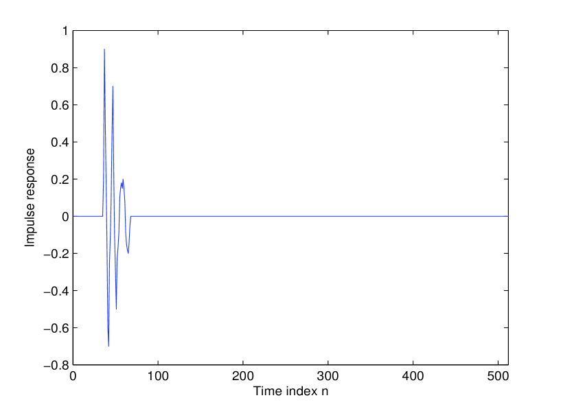
Figure 1: Impulse response of the sparse system

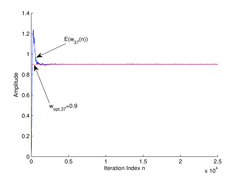
Figure 2: Evolution of $E(w_{37}(n))$ of the ZA-PNLMS algorithm with its optimum level $w_{opt,37}=0.9$.

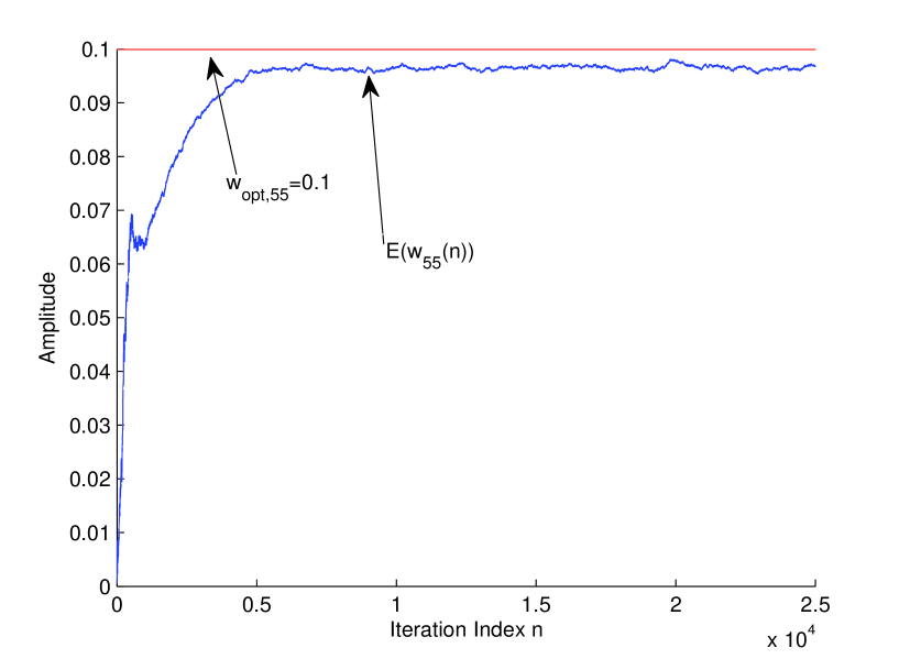
Figure 3: Evolution of $E(w_{55}(n))$ of the ZA-PNLMS algorithm with its optimum level $w_{opt,55}=0.1$.

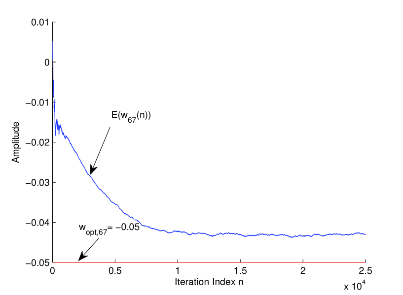
Figure 4: Evolution of $E(w_{67}(n))$ of the ZA-PNLMS algorithm with its optimum level $w_{opt,67}=-0.5$.

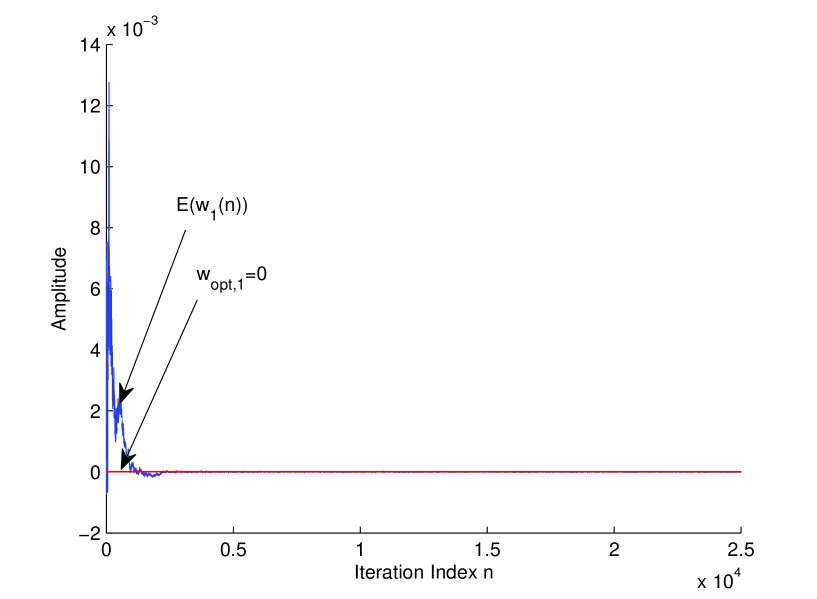
Figure 5: Evolution of $E(w_{1}(n))$ of the ZA-PNLMS algorithm with its optimum level $w_{opt,1}=0$.

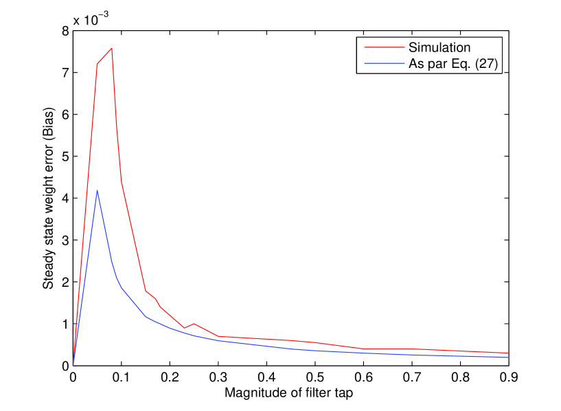
Figure 6: Evolution of $E(w_{1}(n))$ of the ZA-PNLMS algorithm with its optimum level $w_{opt,1}=0$.

References

- [1] J. Radecki, Z. Zilic, and K. Radecka,“Echo cancellation in IP networks”, Proceedings of the 45th Midwest Symposium on Circuits and Systems, vol. 2, pp. 219-222, Tulsa, Okla, USA, August 2002.
- [2] V. V. Krishna, J. Rayala and B. Slade,“Algorithmic and Implementation Apsects of Echo Cancellation in Packet Voice Networks”, Proc. Thirty-Sixth Asilomar Conference on Signals, Systems and Computers, vol. 2, pp. 1252-1257, 2002.
- [3] E. Hansler and G. Schmidt, Eds., Topics in Acoustic Echo and Noise Control, Berlin, Springer-Verlag, 2006.
- [4] W. Schreiber, “Advanced Television Systems for Terrestrial Broadcasting”, Proc. IEEE, vol. 83, no. 6, pp. 958-981, 1995.
- [5] W. Bajwa, J. Haupt, G. Raz and R. Nowak, “Compressed Channel Sensing”, Prof. IEEE CISS, 2008, pp. 5-10.
- [6] M. Kocic, D. Brady and M. Stojanovic, “Sparse Equalization for Real-Time Digital Underwater Acoustic Communications”, Proc. IEEE OCEANS, 1995, pp. 1417-1422.
- [7] R. L. Das and M. Chakraborty, “Sparse Adaptive Filters - an Overview and Some New Results”, Proc. ISCAS-2012, pp. 1267-1270, COEX, Seoul, Korea, May 20-23, 2012.
- [8] D.L. Duttweiler, “Proportionate normalized least-mean-squares adaptation in echo cancelers”, IEEE Trans. Speech Audio Process., vol. 8, no. 5, pp. 508-518, September 2000.
- [9] S. Haykin, Adaptive Filter Theory, Englewood Cliffs, NJ: Prentice-Hall, 1986.
- [10] S.L. Gay, “An efficient, fast converging adaptive filter for network echo cancellation”, Proc. Asilomar Conf. Signals, Systems, Comput., pp. 394-398, Nov., 1998.
- [11] J. Benesty and S.L. Gay,“An improved PNLMS algorithm”, Proceedings of the IEEE International Conference on Acoustic, Speech and Signal Processing , pp. 1881-1884, 2002, Orlando, Florida, USA.
- [12] M. A. Mehran Nekuii, “A Fast Converging Algorithm for Network Echo Cancelation”, IEEE Signal Processing Letters, vol. 11, no. 4, pp. 427-430, April, 2004.
- [13] H. Deng and M. Doroslovacki, “Improving convergence of the PNLMS algorithm for sparse impulse response identification”, IEEE Signal Processing Letters, vol. 12, no. 3, pp. 181-184, 2005.
- [14] L. Liu, M. Fukumoto, S. Saiki and S. Zhang, “ A Variable Step-Size Proportionate Affine Projection Algorithm for Identification of Sparse Impulse Response”, EURASIP Journal on Advances in Signal Processing , pp. 1-10, 2009.
- [15] L. Liu, M. Fukumoto, S. Saiki and S. Zhang, “ A Variable Step-Size Proportionate NLMS Algorithm for Identification of Sparse Impulse Response”, IEICE Trans. Fundamentals, vol. E93–A, no. 1, Jan. 2010.
- [16] C. Paleologu, J. Benesty, F. Albu and S. Ciochinǎ, “ An Efficient Variable Step-Size Proportionate Affine Projection Algorithm” , Proc. IEEE ICASSP, pp. 77-80, 2011.
- [17] Y. Chen, Y. Gu, and A.O. Hero,“Sparse LMS for system identification” , Proc. IEEE ICASSP-2009, pp. 3125-3128, Apr. 2009, Taipei, Taiwan.
- [18] Y. Chen, Y. Gu, and A.O. Hero,“Regularized Least-Mean-Square Algorithms”, Arxiv preprint arXiv:1012.5066v2[stat.ME], Dec. 2010.
- [19] R. L. Das and M. Chakraborty, “A Zero Attracting Proportionate Nor- malized Least Mean Square Algorithm”, Proc. APSIPA-ASC-2012, pp. 1-4, Hollywood, California, 3-6 Dec. 2012.
- [20] R. L. Das and M. Chakraborty, “A Variable Step-Size Zero Attracting Proportionate Normalized Least Mean Square Algorithm”, Proc. ISCAS-2014, COEX, Melbourne, Australia, June 1-5, 2014.
- [21] M. Yukawa and I. Yamada, “A unified view of adaptive variable - metric projection algorithms”, EURASIP Journal on Advances in Signal Processing, vol. 2009, pp. 1-13, 2009.
- [22] D. T. M. Slock, “On the convergence behavior of the lms and the normalized lms algorithms”, IEEE Trans. on Signal Processing, vol. 41, no. 9, pp. 2811-2825, Sep. 1993.
- [23] Z. Yang, Y. R. Zheng and S. L. Grant, “Proportionate affine projection sign algorithms for network echo cancellation”, IEEE Trans. on Audio, Speech,and Language Processing, vol. 19, no. 8, pp. 2273-2284, Nov. 2011.
- [24] S. G. Sankaran and A. A. (Louis) Beex, “Convergence behavior of affine projection algorithms”, IEEE Trans. on Signal Processing, vol. 48, no. 4, pp. 1086-1096, Apr. 2000.
- [25] T. K. Paul and T. Ogunfunmi, “On the convergence behavior of the affine projection algorithm for adaptive filters”, IEEE Trans. on Circuits and System-1:Regular Papers, vol. 58, no. 8, pp. 1813-1826, Aug. 2011.
- [26] R. L. Das and M. Chakraborty, “On Convergence of Proportionate-type Normalized Least Mean Square Algorithms”, IEEE Trans. Circuits and Systems II: Express Briefs, vol. 62, no. 5, pp. 491-495, May, 2015.
- [27] R. Price, “A useful theorem for nonlinear devices using gaussian inputs,” IRE Trans. on Information Theory, vol. 4, no. 2, pp. 69–72, Jun. 1958.
- [28] A. Papoulis and S. U. Pillai, Probability, Random Variables and Stochastic Processes, 4th ed. New York, NY, USA: McGraw Hill, 2002.
- [29] R. H. Kwong and E. W. Johnston, “A variable step size LMS algorithm”, IEEE Trans. Signal Processing, vol. 40, no. 7, pp. 1633-1642, July 1992.