Open Weak CAD and Its Applications

Abstract

The concept of open weak CAD is introduced. Every open CAD is an open weak CAD. On the contrary, an open weak CAD is not necessarily an open CAD. An algorithm for computing projection polynomials of open weak CADs is proposed. The key idea is to compute the intersection of projection factor sets produced by different projection orders. The resulting open weak CAD often has smaller number of sample points than open CADs.

The algorithm can be used for computing sample points for all open connected components of $f\neq 0$ for a given polynomial $f$. It can also be used for many other applications, such as testing semi-definiteness of polynomials and copositive problems. In fact, we solved several difficult semi-definiteness problems efficiently by using the algorithm. Furthermore, applying the algorithm to copositive problems, we find an explicit expression of the polynomials producing open weak CADs under some conditions, which significantly improves the efficiency of solving copositive problems.

url]www.math.ncsu.edu/~hong

url]www.math.pku.edu.cn/is/~xbc/

1 Introduction

In this paper, we introduce the concept of  open weak CAD, provide an algorithm for computing corresponding projection polynomials, and illustrate its usefulness through various applications. In the following, we elaborate on the above sentence.

Cylindrical Algebraic Decomposition (CAD) is a fundamental concept and tool for computational real algebraic geometry with numerous applications. It was introduced by Collins (1975, 1998) and have been improved by many (McCallum, 1984; Hong, 1990; Collins and Hong, 1991; Hong, 1992; Liska and Steinberg, 1993; Renegar, 1992; Basu et al., 1996; McCallum, 1999; Anai and Weispfenning, 2001; Brown, 2001; Strzebonski, 2006; Hong and Safey El Din, 2012; Chen and Maza, 2014).

For polynomials in $n$ variables, a CAD is a finite collection of sign-invariant cells satisfying the following two requirements : (a) the cells constitute a decomposition of the whole $n$-dimensional space. (b) the cells are cylindrically arranged. Such a decomposition is typically constructed in two stages: (1)  compute a kind of triangular set of polynomials through repeated projection, resulting in so-called projection polynomials (2) carrying back substitutions by repeatedly solving the projection polynomials.

It was immediately observed that the computation of CAD can be time-consuming. Hence there have been intensive and diverse effort to improve its computational efficiency. For instance, it was observed that the algorithms spend huge amount of time on constructing low dimensional cells and that those cells are often not needed in various applications. Hence a relaxed notion called  open CAD or  generic CAD was introduced, where low dimensional cells are ignored. Consequently, it relaxes the requirement (a) that the cells constitute a decomposition of the whole space.

In this paper, we introduce a further relaxed notion called open weak CAD, where we also relax the requirement (b) that the cells are cylindrically arranged. Technically, the cylindricity is intimately related to delineability. We replace the original delineability requirement with a weaker version in such a way that it still captures sufficient amount of geometric information needed in various applications.

Furthermore, we provide an algorithm for computing projection polynomials of open weak CADs. The key idea is to compute the intersection of projection factor sets produced by different projection orders. The resulting open weak CAD often has smaller number of cells than open CADs.

We illustrate the usefulness of open weak CAD theory and algorithm by tackling several application problems. First we show how to compute sample points for all open connected components of $f\neq 0$ for a given polynomial $f$. Next we show how to test polynomial inequalities. Finally we show how to tackle co-positiveness problems; we find an explicit expression of the polynomials producing open weak CADs under some conditions, which significantly improves the efficiency of solving copositive problems.

The structure of this paper is as follows. In Section 2, we introduce a notion of open weak delineability and open weak CAD and then state the problem of finding projection polynomials. In Section 3, we review basic definitions, lemmas and concepts of CAD. In Section 4, we introduce several properties of open weak delineable, provide an algorithm for computing projection polynomials of open weak CADs and prove its correctness. In Section 5, we apply open weak CAD theory and algorithm to compute open sample. In Section 6, we apply open weak CAD theory and algorithm and some previous work (Han et al., 2016) to prove polynomial inequalities. In Section 7, we again apply open weak CAD theory and algorithm to test co-positiveness. Section 8, we provide several examples which demonstrate the effectiveness of the algorithms.

2 Problem: Open weak CAD

In this section, we give a precise statement of the problem. We begin by introducing several notions.

Definition 1 (Open weak delineable).

Let $f\in{\mathbb{R}}[x_{1},\ldots,x_{n}]$ and let $S$ be an open set of ${\mathbb{R}}^{j}(1\leq j<n)$. We say that $f$ is open weak delineable (OWD) on $S$ if, for any open connected component $U\subseteq{\mathbb{R}}^{n}$ defined by $f\neq 0$, we have either

$$S\subseteq\pi_{j}^{n}(U)\,\,\,\text{or}\,\,\,S\cap\pi_{j}^{n}(U)=\emptyset,$$

where $\pi_{j}^{n}(x_{1},\ldots,x_{n})=(x_{1},\ldots,x_{j})$. Let $h\in{\mathbb{R}}[x_{1},\ldots,x_{j}]$ for $j\leq n.$ We say that $f$ is open weak delineable over $h$ in ${\mathbb{R}}^{j}$, if $f$ is open weak delineable on any open connected component of $h\neq 0$ in ${\mathbb{R}}^{j}$.

Example 1.

Let

$$f=(x_{2}^{2}-1)^{2}-x_{1}\in{\mathbb{R}}[x_{1},x_{2}].$$

The plot of $f=0$ is given by

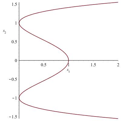
Figure 1: Example 1

Note that $f$ is analytically delineable (Collins (1975), McCallum (1998)) and also open weak delineable on the set $(-\infty,0)$. Note that $f$ is not analytically delineable but is open weak delineable on the set $(0,\infty)$. Note also that $f$ is open weak delineable over $h=x_{1}$ in ${\mathbb{R}}.$

Definition 2 (Open weak CAD).

Let $f\in{\mathbb{R}}[x_{1},\ldots,x_{n}]$. A decomposition of ${\mathbb{R}}^{j}$, $1\leq j<n$, is called an open weak CAD of $f$ in ${\mathbb{R}}^{j}$ if and only if $f$ is open weak delineable on every $j$-dimensional open set in the decomposition.

Example 2.

Let $f$ be the polynomial from Example 1,

$$\{(-\infty,0),[0,0],(0,\infty)\}$$

is an open weak CAD of $f$ in ${\mathbb{R}}$.

Finally, we are ready to state the problem precisely.

Problem. (Projection polynomials of open weak CAD) Devise an algorithm with the following specification.

In:

$f\in{\mathbb{Z}}[x_{1},\ldots,x_{n}]$

Out:

$h_{1},\ldots,h_{n-1}$ where $h_{j}\in{\mathbb{Z}}[x_{1},\ldots,x_{j}]$ such that $f$ is open weak delineable over $h_{j}$ in ${\mathbb{R}}^{j}$.

Example 3.

Consider the following polynomial.

In:

$f=(x_{3}^{2}+x_{2}^{2}+x_{1}^{2}-1)(4x_{3}+3x_{2}+2x_{1}-1)\in{\mathbb{Z}}[x_{1},x_{2},x_{3}]$

Out:

$h_{1}=(x_{1}-1)(x_{1}+1)(29x_{1}^{2}-4x_{1}-24)((20x_{1}^{2}-4x_{1}-15)^{2}+(13x_{1}^{2}-4x_{1}-8)^{2})\in{\mathbb{Z}}[x_{1}]$

$h_{2}=(x_{2}^{2}+x_{1}^{2}-1)(25x_{2}^{2}+12x_{2}x_{1}+20x_{1}^{2}-6x_{2}-4x_{1}-15)\in{\mathbb{Z}}[x_{1},x_{2}]$

The left plot in Figure 2 below shows the open weak CAD of $f$ produced by $h_{1}$ and $h_{2}$. The factor $(20x_{1}^{2}-4x_{1}-15)^{2}+(13x_{1}^{2}-4x_{1}-8)^{2}$ in $h_{1}$ does not have real root and thus it does not contribute to the open weak CAD.

Figure 2: Example 3

Remark 3.

For comparison, if we apply an open CAD algorithm on the above $f$, one would obtain the following output

Out:

$h_{1}=(x_{1}-1)(x_{1}+1)(29x_{1}^{2}-4x_{1}-24)(13x_{1}^{2}-4x_{1}-8)\in{\mathbb{Z}}[x_{1}]$

$h_{2}=(x_{2}^{2}+x_{1}^{2}-1)(25x_{2}^{2}+12x_{2}x_{1}+20x_{1}^{2}-6x_{2}-4x_{1}-15)\in{\mathbb{Z}}[x_{1},x_{2}]$

The right plot in Figure 2 shows the open CAD of $f$ produced by $h_{1}$ and $h_{2}$. Note that it has more cells than the open weak CAD (on the left).

Remark 4.

It is natural to wonder whether the multivariate discriminants of $f$ always produce open weak CADs. Unfortunately, this is not true since the discriminant ${\rm discrim}(f,[x_{n},\ldots,x_{j+1}])$ (the multivariate discriminant of $f$ with respect to $x_{n},\ldots,x_{j+1}$) may vanish identically and thus does not always produces an open weak CAD of ${\mathbb{R}}^{j}$. One may also wonder whether if the multivariate discriminants of $f$ do produce open weak CADs, then they would be the smallest open weak CADs. Unfortunately this is not true either. In Example 1, it has been shown that $x_{1}$ produces an open weak CAD of ${\mathbb{R}}$ with $2$ open intervals. But the discriminant ${\rm discrim}(f,x_{2})=-256(x_{1}-1)x_{1}^{2}$ produces an open weak CAD of ${\mathbb{R}}$ with $3$ open intervals.

Remark 5.

The output of the above problem is a list of “projection” polynomials, not an open weak CAD. As usual, we can compute sample points in an open weak CAD of $f$ from the projection polynomial $h_{j}$ by standard lifting technique. We say that $h_{j}$ produce an open weak CAD. Thus, in this paper, we will focus ourselves on the problem of finding projection polynomial of Open Weak CAD.

3 Preliminaries

If not specified, for a positive integer $n$, let $\bm{x}_{n}$ be the list of variable $(x_{1},\dots,x_{n})$ and $\bm{\alpha}_{n}$ and $\bm{\beta}_{n}$ denote the point $(\alpha_{1},\dots,\alpha_{n})\in{\mathbb{R}}^{n}$ and $(\beta_{1},\dots,\beta_{n})\in{\mathbb{R}}^{n}$, respectively.

Definition 6.

Let $f\in{\mathbb{Z}}[\bm{x}_{n}]$, denote by ${\rm lc}(f,x_{i})$ and ${\rm discrim}(f,x_{i})$ the leading coefficient and the discriminant of $f$ with respect to (w.r.t.) $x_{i}$, respectively. The set of real zeros of $f$ is denoted by ${\rm Zero}(f)$. Denote by ${\rm Zero}(L)$ or ${\rm Zero}(f_{1},\ldots,f_{m})$ the common real zeros of $L=\{f_{1},\ldots,f_{m}\}\subset{\mathbb{Z}}[\bm{x}_{n}].$ The level for $f$ is the biggest $j$ such that $\deg(f,{x_{j}})>0$ where $\deg(f,x_{j})$ is the degree of $f$ w.r.t. $x_{j}$. For polynomial set $L\subseteq{\mathbb{Z}}[\bm{x}_{n}]$, $L^{[i]}$ is the set of polynomials in $L$ with level $i$.

Definition 7.

If $h$$\in{\mathbb{Z}}[\bm{x}_{n}]$ can be factorized in ${\mathbb{Z}}[\bm{x}_{n}]$ as:

$$h=al_{1}^{2j_{1}-1}\cdots l_{t}^{2j_{t}-1}{h_{1}}^{2i_{1}}\cdots{h_{m}}^{2i_{m}},$$

where $a\in{\mathbb{Z}}$, $t\geq 0,m\geq 0$, $l_{i}$$(i=1,\ldots,t)$ and $h_{i}$$(i=1,\ldots,m)$ are pairwise different irreducible primitive polynomials with positive leading coefficients $($under a suitable ordering$)$ and positive degrees in ${\mathbb{Z}}[\bm{x}_{n}]$, then define

$${\rm sqrfree}(h)=l_{1}\cdots l_{t}{h_{1}}\cdots{h_{m}},$$

$${\rm sqrfree}_{1}(h)=\{l_{i},i=1,2,\ldots,t\},$$

$${\rm sqrfree}_{2}(h)=\{h_{i},i=1,2,\ldots,m\}.$$

If $h$ is a constant, let ${\rm sqrfree}(h)=1,$ ${\rm sqrfree}_{1}(h)={\rm sqrfree}_{2}(h)=\{1\}.$

In the following, we introduce some basic known concepts and results of CAD. The reader is referred to Collins (1975); Hong (1990); Collins and Hong (1991); McCallum (1988, 1998); Brown (2001) for a detailed discussion on the properties of CAD.

Definition 8.

(Collins, 1975; McCallum, 1988) An $n$-variate polynomial $f(\bm{x}_{n-1},x_{n})$ over the reals is said to be delineable on a subset $S$ (usually connected) of ${\mathbb{R}}^{n-1}$ if (1) the portion of the real variety of $f$ that lies in the cylinder $S\times{\mathbb{R}}$ over $S$ consists of the union of the graphs of some $t\geq 0$ continuous functions $\theta_{1}<\cdots<\theta_{t}$ from $S$ to ${\mathbb{R}}$; and (2) there exist integers $m_{1},\ldots,m_{t}\geq 1$ s.t. for every $a\in S$, the multiplicity of the root $\theta_{i}(a)$ of $f(a,x_{n})$ (considered as a polynomial in $x_{n}$ alone) is $m_{i}$.

Definition 9.

(Collins, 1975; McCallum, 1988) In the above definition, the $\theta_{i}$ are called the real root functions of $f$ on $S$, the graphs of the $\theta_{i}$ are called the $f$-sections over $S$, and the regions between successive $f$-sections are called $f$-sectors.

Theorem 10.

(McCallum, 1988, 1998) Let $f(\bm{x}_{n},x_{n+1})$ be a polynomial in ${\mathbb{Z}}[\bm{x}_{n},x_{n+1}]$ of positive degree and ${\rm discrim}(f,x_{n+1})$ is a nonzero polynomial. Let $S$ be a connected submanifold of ${\mathbb{R}}^{n}$ on which $f$ is degree-invariant and does not vanish identically, and in which ${\rm discrim}(f,x_{n+1})$ is order-invariant. Then $f$ is analytic delineable on $S$ and is order-invariant in each $f$-section over $S$.

Based on this theorem, McCallum proposed the projection operator MCproj, which consists of the discriminant of $f$ and all coefficients of $f$.

Theorem 11.

(Brown, 2001) Let $f(\bm{x}_{n},x_{n+1})$ be a $(n+1)$-variate polynomial of positive degree in $x_{n+1}$ such that ${\rm discrim}(f,x_{n+1})$ $\neq 0$. Let $S$ be a connected submanifold of ${\mathbb{R}}^{n}$ in which ${\rm discrim}(f,x_{n+1})$ is order-invariant, the leading coefficient of $f$ is sign-invariant, and such that $f$ vanishes identically at no point in $S$. $f$ is degree-invariant on $S$.

Based on this theorem, Brown obtained a reduced McCallum projection in which only leading coefficients, discriminants and resultants appear. The Brown projection operator is defined as follows.

Definition 12.

(Brown, 2001) Given a polynomial $f\in{\mathbb{Z}}[\bm{x}_{n}]$, if $f$ is with level $n$, the Brown projection operator for $f$ is

$${\tt Bp}(f,[x_{n}])={\rm Res}({\rm sqrfree}(f),\frac{\partial({\rm sqrfree}(f))}{\partial x_{n}},x_{n}).$$

Otherwise, ${\tt Bp}(f,[x_{n}])=f$. If $L$ is a polynomial set with level $n$, then

$${\tt Bp}(L,[x_{n}])= \bigcup_{f\in L}\{{\rm Res}({\rm sqrfree}(f),\frac{\partial({\rm sqrfree}(f))}{\partial x_{n}},x_{n})\}\bigcup$$

$$\bigcup_{f,g\in L,f\neq g}\{{\rm Res}({\rm sqrfree}(f),{\rm sqrfree}(g),x_{n})\}.$$

Define

$${\tt Bp}(f,[x_{n},x_{n-1},\ldots,x_{i}])$$

$$= {\tt Bp}({\tt Bp}(f,[x_{n},x_{n-1},\ldots,x_{i+1}]),[x_{i}]).$$

The following definition of open CAD is essentially the GCAD introduced in Strzeboński (2000). For convenience, we use the terminology of open CAD in this paper.

Definition 13.

$($Open CAD$)$ For a polynomial $f(\bm{x}_{n})\in{\mathbb{Z}}[\bm{x}_{n}]$, an open CAD defined by $f(\bm{x}_{n})$ under the order $x_{1}\prec x_{2}\prec\cdots\prec x_{n}$ is a set of sample points in ${\mathbb{R}}^{n}$ obtained through the following three phases:

1. [Projection] Use the Brown projection operator on $f(\bm{x}_{n})$, let

   $$F=\{f,{\tt Bp}(f,[x_{n}]),\ldots,{\tt Bp}(f,[x_{n},\dots,x_{2}])\};$$

2. [Base] Choose one rational point in each of the open intervals defined by the real roots of $F^{[1]}$;

3. [Lifting] Substitute each sample point of ${\mathbb{R}}^{i-1}$ for $\bm{x}_{i-1}$ in $F^{[i]}$ to get a univariate polynomial $F_{i}(x_{i})$ and then, by the same method as Base phase, choose sample points for $F_{i}(x_{i})$. Repeat the process for $i$ from $2$ to $n$.

Sometimes, we say that the polynomial set $F$ produces the open CAD or simply, $F$ is an open CAD.

4 Open Weak CAD: Properties and Algorithm

In this section, we derive some basic properties of Open weak CAD, describe an algorithm (Algorithm 1) for computing open weak CAD and prove its correctness (Theorem 29).

We first prove two simple but useful properties of open weak delineable. The first one is a transitive property.

Proposition 14.

Let $f_{n}(\bm{x}_{n})\in{\mathbb{Z}}[x_{1},\ldots,x_{n}]$, and $S$ be an open set of ${\mathbb{R}}^{j}(1\leq j<n)$. Suppose that there exists $k(j\leq k\leq n)$ and a polynomial $f_{k}(\bm{x}_{k})\in{\mathbb{Z}}[x_{1},\ldots,x_{k}]$ such that $f_{k}(\bm{x}_{k})$ is open weak delineable on $S$, and $f_{n}(\bm{x}_{n})$ is open weak delineable on $f_{k}(\bm{x}_{k})$. Then $f_{n}(\bm{x}_{n})$ is open weak delineable on $S$.

Proof..

Let $U\subseteq{\mathbb{R}}^{n}$ be any open connected component defined by $f_{n}\neq 0$ such that $\pi_{j}^{n}(U)\cap S\neq\emptyset$. We have $\pi_{j}^{k^{-1}}(S)\cap\pi_{k}^{n}(U)\neq\emptyset$ since $\pi_{j}^{n}(U)=\pi_{k}^{n}(\pi_{j}^{k}(U))$. Let $S^{\prime}\subseteq{\mathbb{R}}^{k}$ be any open connected component defined by $f_{k}\neq 0$ such that $S^{\prime}\cap\pi_{j}^{k^{-1}}(S)\cap\pi_{k}^{n}(U)\neq\emptyset$. Now, $S^{\prime}\subseteq\pi_{k}^{n}(U)$ and $S\subseteq\pi_{j}^{k}(S^{\prime})$ since $f_{n}(\bm{x}_{n})$ is open weak delineable on $f_{k}(\bm{x}_{k})$, and $f_{k}(\bm{x}_{k})$ is open weak delineable on $S$. Hence, $\pi_{j}^{n}(U)\supseteq\pi_{j}^{k}(S^{\prime})\supseteq S$.    $\Box$

Before stating the next property, let us take an example to illustrate our motivation. Let $f(x,y,z)=x^{2}+y^{2}\in{\mathbb{Z}}[x,y,z]$. In this case $f\neq 0$ has only one open component $U=\{(x,y)\in{\mathbb{R}}^{2}|x^{2}+y^{2}\neq 0\}$. Let $S_{1}=\{(x,y)\in{\mathbb{R}}^{2}|x>0\}$, $S_{2}=\{(x,y)\in{\mathbb{R}}^{2}|x<0\}$, $S_{3}=\{(x,y)\in{\mathbb{R}}^{2}|y>0\}$, $S_{4}=\{(x,y)\in{\mathbb{R}}^{2}|y<0\}$. It is clear that $S_{i}\subseteq\pi_{2}^{3}(U)$ $(i=1,\ldots,4)$, and $f$ is OWD over $x$ ($y$) in ${\mathbb{R}}^{2}$, respectively. Since $\cup_{i=1}^{4}S_{i}\subseteq\pi_{2}^{3}(U)$ and $\cup_{i=1}^{4}S_{i}=({\mathbb{R}}^{2}\backslash{\rm Zero}(x))\cup({\mathbb{R}}^{2}\backslash{\rm Zero}(y))={\mathbb{R}}^{2}\backslash{\rm Zero}(x,y)={\mathbb{R}}^{2}\backslash{\rm Zero}(x^{2}+y^{2})$, $f$ is OWD over $x^{2}+y^{2}$. We note that $f$ is not OWD over $\gcd(x,y)=1$, while ${\rm Zero}(\gcd(x,y))$ and ${\rm Zero}(x^{2}+y^{2})$ only differ at a closed set of codimension $2$. In general, we have the following Proposition.

Proposition 15.

Let $f(\bm{x}_{n})\in{\mathbb{Z}}[\bm{x}_{n}]$, suppose $f$ is OWD over $p_{1},\ldots,p_{t}$ in ${\mathbb{R}}^{j}$, $f$ is OWD over $p^{\prime}=\sum_{i=1}^{t}p_{i}^{2}$ in ${\mathbb{R}}^{j}$.

Proof..

Let $S\subseteq{\mathbb{R}}^{j}$ be any open connected component defined by $p^{\prime}\neq 0$, $U\subseteq{\mathbb{R}}^{n}$ be any open connected set defined by $f\neq 0$. Let $S_{1}=\{\bm{\alpha}|\bm{\alpha}\in S,(\bm{\alpha}\times{\mathbb{R}}^{n-j})\cap U\neq\emptyset\}$, $S_{2}=\{\bm{\alpha}|\bm{\alpha}\in S,(\bm{\alpha}\times{\mathbb{R}}^{n-j})\cap U=\emptyset\}$. It is clear that $S=S_{1}\cup S_{2}$, $S_{1}\cap S_{2}=\emptyset$. For any $\bm{\alpha}\in S$, we assume that $p_{1}(\bm{\alpha})\neq 0$. There exists an open set $S_{\bm{\alpha}}\subseteq{\mathbb{R}}^{j}$ containing $\bm{\alpha}$, such that $p_{1}(S_{\bm{\alpha}})\neq 0$. Since $f$ is OWD over $p_{1}$, either $S_{\bm{\alpha}}\subseteq S_{1}$ or $S_{\bm{\alpha}}\subseteq S_{2}$. Hence, either $S=S_{1}$ or $S=S_{2}$ since $S$ is a connected set, and it can not be partitioned into two nonempty subsets which are open. Therefore, $f$ is OWD on $S$, and $f$ is OWD over $p^{\prime}$.    $\Box$

Now the following two theorems follow immediately from the above Propositions. The first one states that the set

$${\rm OWD}^{j}(f)=\{h_{j}\in{\mathbb{Z}}[\bm{x}_{j}]|f\text{ is open weak delineable over }h_{j}\text{ in }{\mathbb{R}}^{j}\}.$$

is nonempty, so the problem proposed in Section 2 makes sense.

Theorem 16.

Let $f(\bm{x}_{n})\in{\mathbb{Z}}[\bm{x}_{n}]$, $f$ is OWD over ${\tt Bp}(f,[x_{n},\ldots,x_{j}])$ in ${\mathbb{R}}^{j-1}$. As a result, the set ${\rm OWD}^{j}(f)$ is nonempty.

Proof..

By Theorem 10 and Theorem 11, $f$ is OWD over ${\tt Bp}(f,[x_{n}])$, and ${\tt Bp}(f,[x_{n},\ldots,x_{i}])$ is OWD over ${\tt Bp}(f,[x_{n},\ldots,x_{i+1}])$ ($j-1\leq i\leq n$). By Proposition 14, $f$ is OWD over ${\tt Bp}(f,[x_{n},\ldots,x_{j}])$ in ${\mathbb{R}}^{j-1}$.    $\Box$

The next theorem says that there is a minimal element in ${\rm OWD}^{j}(f)$ in some sense. In the following, we call the number of the open components in ${\mathbb{R}}^{j}$ defined by $p\neq 0$ the scale of the open weak CAD of $f$ defined by $p$ in ${\mathbb{R}}^{j}$.

Theorem 17.

Let $f(\bm{x}_{n})\in{\mathbb{Z}}[\bm{x}_{n}]$, there exists $p\in{\rm OWD}^{j}(f)$, such that any $p^{\prime}\in{\rm OWD}^{j}(f)$, ${\rm Zero}(p)\subseteq{\rm Zero}(p^{\prime})$. In particular, the scale of the open weak CAD of $f$ defined by $p$ in ${\mathbb{R}}^{j}$ is minimal.

Proof..

Otherwise, for any $p\in{\rm OWD}^{j}(f)$, there exists $p^{\prime}\in{\rm OWD}^{j}(f)$ such that ${\rm Zero}(p^{2}+p^{\prime 2})={\rm Zero}(p)\cap{\rm Zero}(p^{\prime})\subsetneq{\rm Zero}(p)$. By Proposition 15, $p^{2}+p^{\prime 2}\in{\rm OWD}^{j}(f)$. Thus, we can find a sequence of polynomials $p_{i}\in{\rm OWD}^{j}(f)$ ($i=1,2,\ldots$), such that the descending chain of closed sets ${\rm Zero}(p_{1})\supsetneq{\rm Zero}(p_{2})\supsetneq\cdots$ is not stationary, which contradicts with the well-known fact that ${\mathbb{R}}^{j}$ is noetherian under the Zariski Topology.    $\Box$

We want to obtain an element in ${\rm OWD}^{j}(f)$ as small as possible. A natural way is to apply Theorem 16 and Proposition 15. Let us take $f\in{\mathbb{Z}}[x,y,z,w]$ as an example. According to Theorem 16, $f$ is OWD over $p_{1}={\tt Bp}(f,[w,z])$ and $p_{2}={\tt Bp}(f,[z,w])$ in ${\mathbb{R}}^{2}$, respectively. According to Proposition 15, $f$ is OWD over $p^{\prime}=p_{1}^{2}+p_{2}^{2}$ in ${\mathbb{R}}^{2}$. If we want to obtain an element in ${\rm OWD}^{1}(f)$ from $p^{\prime}$, the simplest way is to apply Brown’s projection operator directly, ${\tt Bp}(p^{\prime},y)\in{\rm OWD}^{1}(f)$. But it is quite possible that ${\tt Bp}(p^{\prime},y)$ is more complicated than ${\tt Bp}(f,[w,z,y])$, since the degree of $p^{\prime}$ is twice as much as that of ${\tt Bp}(f,[w,z])$. For a polynomial $p\in{\mathbb{Z}}[x,y]$, whether $p\in{\rm OWD}^{2}(f)$ or not is only dependent on the real zeros of $p$. It indicates us that, instead of computing ${\tt Bp}(p^{\prime},y)$ directly, we may find a polynomial $p\in{\mathbb{Z}}[x,y]$, such that ${\rm Zero}(p)$ and ${\rm Zero}(p^{\prime})$ are almost the same, and ${\tt Bp}(p,y)\in{\rm OWD}^{1}(f)$. Roughly speaking, let $p=\gcd(p_{1},p_{2})$, $p_{1}^{\prime}=\frac{p_{1}}{p}$, $p_{2}^{\prime}=\frac{p_{2}}{p}$. For simplicity, we suppose that $p$ is an irreducible polynomial. It is clear that ${\rm Zero}(p_{1}^{2}+p_{2}^{2})={\rm Zero}(p(p_{1}^{\prime 2}+p_{2}^{\prime 2}))={\rm Zero}(p)\cup{\rm Zero}(p_{1}^{\prime 2}+p_{2}^{\prime 2})$. Since $\gcd(p_{1}^{\prime},p_{2}^{\prime})=1$, intuitively, ${\rm Zero}(p_{1}^{\prime 2}+p_{2}^{\prime 2})={\rm Zero}(p_{1}^{\prime},p_{2}^{\prime})$ is a closed set of codimension $2$. If $p$ is not semi-definite, one can show that ${\rm Zero}(p)$ is a closed set of codimension $1$. Thus, the two sets ${\rm Zero}(p)$ and ${\rm Zero}(p^{\prime})$ are almost the same. We will show that $f$ is “almost” OWD over ${\tt Bp}(p,y)$ in ${\mathbb{R}}^{1}$.

In order to state our results precisely, we introduce the following definitions.

Definition 18.

Let $Q=\{q_{1},\ldots,q_{s}\}$ be a polynomial set, where $q_{i}\neq 0$. We say that $Q$ is a polynomial set of level $j$ if $q_{i}\in{\mathbb{R}}[x_{1},\ldots,x_{j}]$. Define

$$Q^{2}=\sum_{i=1}^{s}q_{i}^{2}.$$

Let $\bm{\alpha}\in{\mathbb{R}}^{j}$, define

$$Q(\bm{\alpha})=\{q_{i}(\bm{\alpha})|i=1,\ldots,s\}.$$

It is clear that $\bm{\alpha}\in{\rm Zero}(Q)$ if and only if $Q(\bm{\alpha})=\{0\}$.

Let $\bm{x}_{I}=(x_{i_{1}},\ldots,x_{i_{l}})$, where $1\leq i_{1}<i_{2}<\ldots<i_{l}\leq j$. Define ${\rm coeffs}(Q,[\bm{x}_{I}])$ to be the set of all the coefficients of all the polynomials $q_{i}$ in $Q$ with respect to the indeterminates $\bm{x}_{I}$.

Let $p\in{\mathbb{R}}[x_{1},\ldots,x_{j}],$ define

$$pQ=\{pq_{1},\ldots,pq_{s}\}.$$

We say that a polynomial $g\in{\mathbb{R}}[x_{1},\ldots,x_{n}]$ is a common factor of $Q$, if $g$ is a factor of $q_{i}$ for every $i$.

We say that a polynomial set $Q$ of level $j$ has codimension at least two and denote it by ${\rm codim}(Q)\geq 2$, if for any open connected set $U\subseteq{\mathbb{R}}^{j}$, $U\backslash{\rm Zero}(Q)$ is still open connected.

Lemma 21 below gives a description of a polynomial set of codimension at least two. Before proving the lemma, we introduce the following result.

Lemma 19.

(Han et al., 2016) We have

1. Let $f$ and $g$ be coprime in ${\mathbb{R}}[\bm{x}_{n}]$. For any connected open set $U$ of ${\mathbb{R}}^{n}$, the open set $V=U\backslash{\rm Zero}(f,g)$ is also connected.

2. Suppose $f\in{\mathbb{R}}[\bm{x}_{n}]$ is a non-zero squarefree polynomial and $U$ is a connected open set of $\mathbb{R}^{n}$. If $f(\bm{x}_{n})$ is semi-definite on $U$, then $U\backslash{\rm Zero}(f)$ is also a connected open set.

Lemma 20.

Let $f=\gcd(f_{1},\ldots,f_{m})$ where $f_{i}\in{\mathbb{R}}[\bm{x}_{n}]$, $i=1,2,\ldots,m.$ Suppose $f$ has no real zeros in a connected open set $U\subseteq{\mathbb{R}}^{n}$, then the open set $V=U\backslash{\rm Zero}(f_{1},\ldots,f_{m})$ is also connected.

Proof..

Without loss of generality, we may assume that $f=1$. If $m=1,$ the result is obvious. The result of case $m=2$ is just the claim of Lemma 19. For $m\geq 3$, let $g=\gcd(f_{1},\ldots,f_{m-1})$ and $g_{i}=f_{i}/g$ $(i=1,\ldots,m-1)$, then $\gcd(f_{m},g)=1$ and $\gcd(g_{1},\ldots,g_{m-1})=1$. Let $A={\rm Zero}(f_{1},\ldots,f_{m})$, $B={\rm Zero}(g_{1},\ldots,g_{m-1})\bigcup{\rm Zero}(g,f_{m})$. Since $A\subseteq B$, we have $U\backslash B\subseteq U\backslash A$. Notice that the closure of ${U\backslash B}$ equals the closure of ${U\backslash A}$, it suffices to prove that $U\backslash B$ is connected, which follows directly from Lemma 19 and the induction.    $\Box$

Lemma 21.

Let $Q=\{q_{1},\ldots,q_{s}\}$ be a polynomial set of level $j$. ${\rm codim}(Q)\geq 2$ if and only if for any common factor $g$ of $Q$, $g$ is semi-definite on ${\mathbb{R}}^{n}$.

Proof..

If ${\rm codim}(Q)\geq 2$, $U\backslash{\rm Zero}(Q)$ is connected for any open connected set $U\subseteq{\mathbb{R}}^{j}$. It is obvious that ${\rm Zero}(g)\subseteq{\rm Zero}(Q)$, and

$$U\backslash{\rm Zero}(Q)\subseteq U\backslash{\rm Zero}(g).$$

Notice that the closure of $U\backslash{\rm Zero}(g)$ equals the closure of $U\backslash{\rm Zero}(Q)$, $U\backslash{\rm Zero}(g)$ is open connected. In particular, ${\mathbb{R}}^{j}\backslash{\rm Zero}(g)$ is open connected, and $g$ is semi-definite on ${\mathbb{R}}^{j}$ since $g$ is sign invariant on ${\mathbb{R}}^{j}\backslash{\rm Zero}(g)$.

If for any common factor $g$ of $Q$, $g$ is semi-definite on ${\mathbb{R}}^{n}$. Let $q=\gcd(q_{1},\ldots,q_{s})$, $V=U\backslash{\rm Zero}(q)$, $q_{i}=qq_{i}^{\prime}$, $Q^{\prime}=\{q_{1}^{\prime},\ldots,q_{s}^{\prime}\}$. By assumption, $q$ is semi-definite on ${\mathbb{R}}^{n}$, and $V$ is open connected by Lemma 19. According to Lemma 20,

$$U\backslash{\rm Zero}(Q)=V\backslash{\rm Zero}(Q^{\prime})$$

is open connected since $\gcd(q_{1}^{\prime},\ldots,q_{s}^{\prime})=1$.    $\Box$

By Lemma 21, any common factor $g$ of a polynomial set $Q$ of codimension at least 2 is semi-definite, by Theorem 4.5.1 in (Bochnak et al., 2013), $\dim({\rm Zero}(g))\leq j-2$. In fact, we can show that $\dim({\rm Zero}(Q))\leq j-2$. That’s why we call $Q$ has codimension at least 2.

Definition 22.

Let $f\in{\mathbb{R}}[x_{1},\ldots,x_{n}]$, $p\in{\mathbb{R}}[x_{1},\ldots,x_{j}]$ for $1\leq j\leq n,$ and $Q=\{q_{1},\ldots,q_{s}\}$ is a polynomial set of level $j$, $q_{i}\neq 0$. We say that $f$ is OWD over $p$ w.r.t. $Q$ (in ${\mathbb{R}}^{j}$), if for any open connected component $S$ of $p\neq 0$ in ${\mathbb{R}}^{j}$, $f$ is OWD on $S\backslash{\rm Zero}(Q)$. We also say that $f$ is OWD over $p$ in general.

Remark 23.

If $f$ is OWD over $p$, it is clear that $f$ is OWD over $p$ w.r.t. $\{1\}$. If $f$ is OWD over $p$ w.r.t. $Q_{1}$, and ${\rm Zero}(Q_{1})\subseteq{\rm Zero}(Q_{2})$, by definition, $f$ is OWD over $p$ w.r.t. $Q_{2}$ since $f$ is OWD on $S\backslash{\rm Zero}(Q_{2})\subseteq S\backslash{\rm Zero}(Q_{1})$ for any open connected component $S$ of $p\neq 0$ in ${\mathbb{R}}^{j}$. In particular, if $f$ is OWD over $p$ (w.r.t. $\{1\}$), $f$ is OWD over $p$ w.r.t. $Q$ for any polynomial set $Q$ of level $j$.

The following lemma shows that the above definition is just a variant of OWD when ${\rm codim}(Q)\geq 2$. In the rest of this paper, we will switch the two notations freely.

Lemma 24.

Let $f\in{\mathbb{R}}[x_{1},\ldots,x_{n}]$, $p\in{\mathbb{R}}[x_{1},\ldots,x_{j}]$, $Q$ is a polynomial set of level $j$. If $f$ is OWD over $p$ w.r.t. $Q$, $f$ is OWD over $pQ^{2}$. If ${\rm codim}(Q)\geq 2$, $f$ is OWD over $pQ^{2}$ if and only if $f$ is OWD over $p$ w.r.t. $Q$.

Proof..

If $f$ is OWD over $p$ w.r.t. $Q$. Let $S^{\prime}$ be any open connected component of $pQ^{2}\neq 0$, there there exists a unique open connected component $S$ of $p\neq 0$, such that $S^{\prime}\subseteq S$. Since $Q^{2}(S^{\prime})\neq 0$, $S^{\prime}\subseteq S\backslash{\rm Zero}(Q)$. $f$ is OWD on $S^{\prime}$ since $f$ is OWD on $S\backslash{\rm Zero}(Q)$.

If ${\rm codim}(Q)\geq 2$, and $f$ is OWD over $pQ^{2}$. Let $S$ be any open connected component of $p\neq 0$, and $S^{\prime}$ be any open connected component of $pQ^{2}\neq 0$, such that $S^{\prime}\subseteq S$. We have $S^{\prime}\subseteq S\backslash{\rm Zero}(Q)$. Now $pQ^{2}(S\backslash{\rm Zero}(Q))\neq 0$, and $S\backslash{\rm Zero}(Q)$ is open connected since ${\rm codim}(Q)\geq 2$. Thus, $S\backslash{\rm Zero}(Q)\subseteq S^{\prime}$. Hence, $S\backslash{\rm Zero}(Q)=S^{\prime}$, and $f$ is OWD on $S\backslash{\rm Zero}(Q)$.    $\Box$

The following two theorems are analogous to Proposition 14 and Proposition 15.

Theorem 25.

Let $f\in{\mathbb{R}}[\bm{x}_{n}]$, $1\leq j<k<n$, $p_{1}\in{\mathbb{R}}[\bm{x}_{k}]$, $p_{2}\in{\mathbb{R}}[\bm{x}_{j}]$, $Q_{1}$ is a polynomial set of level $k$. Suppose $f$ is OWD over $p_{1}$ w.r.t. $Q_{1}$, and $p_{1}$ is OWD over $p_{2}$. $f$ is OWD over $p_{2}$ w.r.t. $Q_{2}={\rm coeffs}(Q_{1},[x_{k},\ldots,x_{j+1}])$. Furthermore, if ${\rm codim}(Q_{1})\geq 2$, ${\rm codim}(Q_{2})\geq 2.$

Proof..

Let $S^{\prime\prime}\subseteq{\mathbb{R}}^{j}$ be any open component of $p_{2}\neq 0$, $S=S^{\prime\prime}\backslash{\rm Zero}(Q_{2})$. We prove that $f$ is OWD on $S$. Let $U\subseteq{\mathbb{R}}^{n}$ be any open component of $f\neq 0$, suppose $S\cap\pi_{j}^{n}(U)\neq\emptyset$. It is clear that $\pi_{j}^{k^{-1}}(S)\cap\pi_{k}^{n}(U)\neq\emptyset$. Let $S^{\prime}\subseteq{\mathbb{R}}^{k}$ be any open component of $p_{1}\neq 0$, such that $(S^{\prime}\cap\pi_{j}^{k^{-1}}(S))\cap\pi_{k}^{n}(U)\neq\emptyset$. $(S^{\prime}\backslash{\rm Zero}(Q_{1}))\cap\pi_{k}^{n}(U)\neq\emptyset$ is nonempty since $S^{\prime}\cap\pi_{k}^{n}(U)$ is a nonempty open set. Thus, $S^{\prime}\backslash{\rm Zero}(Q_{1})\subseteq\pi_{k}^{n}(U)$ since $f$ is OWD over $p_{1}$ w.r.t. $Q_{1}$. We only need to show that $S\subseteq\pi_{j}^{k}(S^{\prime}\backslash{\rm Zero}(Q_{1}))$. Since $S\cap\pi_{j}^{k}(S^{\prime})\neq\emptyset$ and $p_{1}$ is OWD over $p_{2}$, $S\subseteq S^{\prime\prime}\subseteq\pi_{j}^{k}(S^{\prime})$. For any $\bm{\alpha}\in S$, let $\bm{\beta}\in{\mathbb{R}}^{k-j}$ such that $(\bm{\alpha},\bm{\beta})\in S^{\prime}$. $Q_{2}^{2}(\bm{\alpha})\neq 0$ implies that $Q_{2}(\bm{\alpha})\neq\{0\}$. Thus, there exists a polynomial $q\in Q_{2}$, such that $q(\bm{\alpha},x_{j+1},\ldots,x_{k})\neq 0$. Let $U_{\bm{\beta}}\subseteq{\mathbb{R}}^{k-j}$ be a neighborhood of $\bm{\beta}$, such that $(\bm{\alpha},U_{\bm{\beta}})\in S^{\prime}$, $Q_{1}(\bm{\alpha},U_{\bm{\beta}})\neq\{0\}$, and $(\bm{\alpha},U_{\bm{\beta}})\cap(S^{\prime}\backslash{\rm Zero}(Q_{1}))\neq\emptyset$. This indicates that $\bm{\alpha}\in\pi_{j}^{k}(S^{\prime}\backslash{\rm Zero}(Q_{1})).$

If ${\rm codim}(Q_{1})\geq 2$, let $g$ be any common factor of $Q_{2}$. It is clear that $g$ is a common factor of $Q_{1}$. Since ${\rm codim}(Q_{1})\geq 2$, $g$ is semi-definite on ${\mathbb{R}}^{k}$ by Lemma 21. By Lemma 21 again, ${\rm codim}(Q_{2})\geq 2$. The theorem is proved.    $\Box$

As a special case of Theorem 25, when $k=j+1$, and the set $Q_{=}\{q_{1}\}$ has only one polynomial. $f$ is OWD over $p_{2}$ w.r.t. $Q_{2}={\rm coeffs}(\{q_{1}\},[x_{k}])$. In particular, $f$ is OWD over $p_{2}$ w.r.t. ${\rm lc}(q_{1},x_{k})$.

One benefit of Theorem 25 is that we can reduce the computational complexity when we apply Brown’s projection operator. Namely, suppose $k=j+1$, $f$ is OWD over $p_{1}q_{1}$, where $q_{1}$ is an irreducible polynomial and is semi-definite on ${\mathbb{R}}^{k}$. If we apply Brown’s projection operator directly, $f$ is OWD over ${\tt Bp}(p_{1}q_{1},x_{k})$. Now we use Theorem 25 to get a simpler but stronger result. By Lemma 24, $f$ is OWD over $p_{1}$ w.r.t. $q_{1}$. According to Theorem 25, $f$ is OWD over ${\tt Bp}(p_{1},x_{k})$ w.r.t. ${\rm lc}(q_{1},x_{k})$. By Lemma 24 again, $f$ is OWD over ${\rm lc}(q_{1},x_{k}){\tt Bp}(p_{1},x_{k}),$ which is a factor of ${\tt Bp}(p_{1}q_{1},x_{k})$.

Theorem 26.

Let $f\in{\mathbb{R}}[\bm{x}_{n}]$, $p_{i}\in{\mathbb{R}}[\bm{x}_{j}]$, $Q_{i}$ is a polynomial set of level $j$ ($i=1,2,\ldots,t$), $p=\gcd(p_{1},\ldots,p_{t})$, $p_{i}^{\prime}=\frac{p_{i}}{p}$. Suppose $f$ is OWD over $p_{i}$ w.r.t. $Q_{i}$. $f$ is OWD over $p$ w.r.t. $Q=\bigcup_{i=1}^{t}p_{i}^{\prime}Q_{i}$, and ${\rm Zero}(pQ^{2})\subseteq{\rm Zero}(p_{i}Q_{i}^{2})$ for any $i$. Furthermore, if ${\rm codim}(Q_{i})\geq 2$, ${\rm codim}(Q)\geq 2$.

Proof..

Let $S$ be any open connected component defined by $p\neq 0$, $\mathcal{A}_{i}$ be the set of open components of $p_{i}\neq 0$ in $S$. By definition, $S\backslash{{\rm Zero}(p_{i})}=\bigcup_{S_{i}\in\mathcal{A}_{i}}S_{i}$, and

Let $U\subseteq{\mathbb{R}}^{n}$ be any open connected set defined by $f\neq 0$,

$$\mathcal{B}_{i}=\{S_{i}|S_{i}\in\mathcal{A}_{i},S_{i}\backslash{{\rm Zero}(Q_{i})}\subseteq\pi_{j}^{n}(U)\},$$

$$\mathcal{C}_{i}=\{S_{i}|S_{i}\in\mathcal{A}_{i},S_{i}\backslash{{\rm Zero}(Q_{i})}\cap\pi_{j}^{n}(U)=\emptyset\}.$$

Since $f$ is OWD over $p_{i}$ w.r.t. $Q_{i}$, $\mathcal{A}_{i}=\mathcal{B}_{i}\cup\mathcal{C}_{i}$. For any $S^{\prime}\in\mathcal{B}_{i}$, and $S^{\prime\prime}\in\mathcal{C}_{j}$, $S^{\prime}\cap S^{\prime\prime}=\emptyset$ since

$$(S^{\prime}\backslash{{\rm Zero}(Q_{i})})\cap(S^{\prime\prime}\backslash{{\rm Zero}(Q_{j})})\subseteq\pi_{j}^{n}(U)\cap(S^{\prime\prime}\backslash{{\rm Zero}(Q_{j})})=\emptyset.$$

Let

$$B=\bigcup_{1\leq i\leq t,S_{i}\in\mathcal{B}_{i}}S_{i},B^{\prime}=\bigcup_{1\leq i\leq t,S_{i}\in\mathcal{B}_{i}}(S_{i}\backslash{{\rm Zero}(Q_{i})}),$$

$$C=\bigcup_{1\leq i\leq t,S_{i}\in\mathcal{C}_{i}}S_{i},C^{\prime}=\bigcup_{1\leq i\leq t,S_{i}\in\mathcal{C}_{i}}(S_{i}\backslash{{\rm Zero}(Q_{i})}).$$

We have $B\cap C=\emptyset$, and

$$S\backslash{{\rm Zero}(p_{1},\ldots,p_{t})}=\bigcup_{1\leq i\leq t}S\backslash{{\rm Zero}(p_{i})}=B\cup C.$$

By Lemma 20, $V=S\backslash{{\rm Zero}(p_{1},\ldots,p_{t})}$ is open connected, and can not be partitioned into two nonempty subsets which are open. Hence, either $B=\emptyset$ or $C=\emptyset$. Since

$$S\backslash{{\rm Zero}(Q)}=\bigcup_{1\leq i\leq t}S\backslash{{\rm Zero}(p_{i}^{\prime}Q_{i})}=\bigcup_{1\leq i\leq t}S\backslash{{\rm Zero}(p_{i}Q_{i})}=B^{\prime}\cup C^{\prime},$$

and $B^{\prime}\subseteq B$, $C^{\prime}\subseteq C$, either $B^{\prime}=\emptyset$ or $C^{\prime}=\emptyset$. Thus, either $S\backslash{{\rm Zero}(Q)}\subseteq\pi_{j}^{n}(U)$ or $(S\backslash{{\rm Zero}(Q)})\cap\pi_{j}^{n}(U)=\emptyset$. Therefore, $f$ is OWD over $p$ w.r.t. $Q$.

We have

$${\rm Zero}(pQ^{2})={\rm Zero}(p)\cup{\rm Zero}(Q^{2})\subseteq{\rm Zero}(p)\cup{\rm Zero}(p_{i}^{\prime}Q_{i}^{2})={\rm Zero}(p_{i}Q_{i}^{2}),$$

for any $i$.

Since $\gcd(p_{1}^{\prime},\ldots,p_{t}^{\prime})=1$, any common factor $g$ of $Q$ must be a common factor of $Q_{i}$ for some $i$. If ${\rm codim}(Q_{i})\geq 2$, by Lemma 21, $g$ is semi-definite on ${\mathbb{R}}^{j}$. By Lemma 21 again, ${\rm codim}(Q)\geq 2$.    $\Box$

We can apply Theorem 25, Theorem 26 and Brown’s projection operator ${\tt Bp}$ to get a weak open CAD with “smaller” scale now. let us take $f\in{\mathbb{Z}}[x,y,z,w]$ again as an example. According to Theorem 16, $f$ is OWD over ${\tt Hp}(f,[w,z],z)={\tt Bp}(f,[w,z])$ and ${\tt Hp}(f,[w,z],w)={\tt Bp}(f,[z,w])$ in ${\mathbb{R}}^{2}$, respectively. Let

$${\tt Hp}(f,[w,z])=\gcd({\tt Hp}(f,[w,z],z),{\tt Hp}(f,[w,z],w)),$$

$${{\tt Hp}^{\vartriangle}(f,[w,z],w)}=\frac{{\tt Hp}(f,[w,z],w)}{{\tt Hp}(f,[w,z])},$$

$${{\tt Hp}^{\vartriangle}(f,[w,z],z)}=\frac{{\tt Hp}(f,[w,z],z)}{{\tt Hp}(f,[w,z])}.$$

According to Theorem 15, $f$ is OWD over ${\tt Hp}(f,[w,z])$ w.r.t.

$${{\tt Hp}^{\ast}(f,[w,z])}=\{{{\tt Hp}^{\vartriangle}(f,[w,z],w)},{{\tt Hp}^{\vartriangle}(f,[w,z],z)}\}$$

in ${\mathbb{R}}^{2}$, and $f$ is OWD over $h_{2}(f)={\tt Hp}(f,[w,z]){{\tt Hp}^{\ast}(f,[w,z])}^{2}$.

According to Theorem 25, $f$ is OWD over

$${\tt Hp}(f,[w,z,y],y)={\tt Bp}({\tt Hp}(f,[w,z]),y)$$

w.r.t.

$${{\tt Hp}^{\ast}(f,[w,z,y],y)}={\rm coeffs}({{\tt Hp}^{\ast}(f,[w,z])},[y])$$

in ${\mathbb{R}}$.

Similarly, we can define

$${\tt Hp}(f,[w,z,y],z),\,{\tt Hp}(f,[w,z,y],w),\,{\tt Hp}(f,[w,z,y]),$$

$${{\tt Hp}^{\ast}(f,[w,z,y],z)},\,{\tt Hp}^{\ast}(f,[w,z,y],w),$$

and

$${{\tt Hp}^{\vartriangle}(f,[w,z,y],y)},{{\tt Hp}^{\vartriangle}(f,[w,z,y],z)},\,{\tt Hp}^{\vartriangle}(f,[w,z,y],w).$$

Define

$${\tt Hp}^{\ast}(f,[w,z,y])= {\tt Hp}^{\vartriangle}(f,[w,z,y],y){\tt Hp}^{\ast}(f,[w,z,y],y)\bigcup$$

$${\tt Hp}^{\vartriangle}(f,[w,z,y],z){\tt Hp}^{\ast}(f,[w,z,y],z)\bigcup$$

$${\tt Hp}^{\vartriangle}(f,[w,z,y],w){\tt Hp}^{\ast}(f,[w,z,y],w)$$

By applying Theorem 26 again, one can show that $f$ is OWD over ${\tt Hp}(f,[w,z,y])$ w.r.t. ${\tt Hp}^{\ast}(f,[w,z,y])$, or equivalently, $f$ is OWD over

$$h_{1}(f)={\tt Hp}(f,[w,z,y]){\tt Hp}^{\ast}(f,[w,z,y])^{2}.$$

This procedure could apply to any polynomial $f\in{\mathbb{Z}}[\bm{x}_{n}]$. In order to present our results in general, we need to introduce open weak CAD projection operator ${\tt Hp}$.

Definition 27 (Open weak CAD projection operator).

Let $f\in{\mathbb{Z}}[x_{1},\ldots,x_{n}]$. For given $m(1\leq m\leq n),$ denote $[\bm{y}]=[y_{1},\dots,y_{m}]$ where $y_{i}\in\{x_{1},\dots,x_{n}\}$ for $1\leq i\leq m$ and $y_{i}\neq y_{j}$ for $i\neq j$. For $1\leq i\leq m$, ${\tt Hp}(f,[\bm{y}],y_{i})$ and ${\tt Hp}(f,[\bm{y}])$ are defined recursively as follows.

$${\tt Bp}(f,[y_{i}]) ={\rm Res}({\rm sqrfree}(f),\frac{\partial{\rm sqrfree}(f)}{\partial y_{i}},y_{i}),$$

$${\tt Hp}(f,[\bm{y}],y_{i}) ={\tt Bp}({\tt Hp}(f,[\hat{\bm{y}}_{i}],[y_{i}]),$$

$${\tt Hp}(f,[\bm{y}]) =\gcd({\tt Hp}(f,[\bm{y}],y_{1}),\ldots,{\tt Hp}(f,[\bm{y}],y_{m})),$$

$${\tt Hp}(f,[~{}]) =f,$$

where $\hat{[\bm{y}]}_{i}=[y_{1},\ldots,y_{i-1},y_{i+1},\ldots,y_{m}]$.

We define ${{\tt Hp}^{\vartriangle}(f,[\bm{y}],y_{i})}$, ${\tt Hp}^{\ast}(f,[\bm{y}],y_{i})$, ${\tt Hp}^{\ast}(f,[\bm{y}])$ recursively as follows.

$${\tt Hp}^{\ast}(f,[~{}]) =\{1\},$$

$${{\tt Hp}^{\ast}(f,[\bm{y}],y_{i})} ={\rm coeffs}({{\tt Hp}^{\ast}(f,[\hat{\bm{y}}_{i}])},y_{i}),$$

$${{\tt Hp}^{\vartriangle}(f,[\bm{y}],y_{i})} =\frac{{\tt Hp}(f,[\bm{y}],y_{i})}{{\tt Hp}(f,[\bm{y}])},$$

$${{\tt Hp}^{\ast}(f,[\bm{y}])} =\bigcup_{i=1}^{m}{{\tt Hp}^{\vartriangle}(f,[\bm{y}],y_{i})}{{\tt Hp}^{\ast}(f,[\bm{y}],y_{i})}.$$

Example 4.

We have

$${\tt Hp}(f,\left[x_{1},x_{2}\right]) =\gcd\left({\tt Hp}\left(f,\left[x_{1},x_{2}\right],x_{1}\right),{\tt Hp}\left(f,\left[x_{1},x_{2}\right],x_{2}\right)\right),$$

$${\tt Hp}\left(f,\left[x_{1},x_{2}\right],x_{1}\right) ={\tt Bp}({\tt Hp}(f,\left[x_{2}\right]),[x_{1}]),$$

$${\tt Hp}\left(f,\left[x_{1},x_{2}\right],x_{2}\right) ={\tt Bp}({\tt Hp}(f,\left[x_{1}\right]),[x_{2}]),$$

$${\tt Hp}(f,\left[x_{2}\right]) ={\tt Hp}(f,[x_{2}],x_{2}),$$

$${\tt Hp}(f,\left[x_{1}\right]) ={\tt Hp}(f,[x_{1}],x_{1}),$$

$${\tt Hp}(f,[x_{2}],x_{2}) =\gcd({\tt Bp}({\tt Hp}(f,[~{}]),[x_{2}])),$$

$${\tt Hp}(f,[x_{1}],x_{1}) =\gcd({\tt Bp}({\tt Hp}(f,[~{}]),[x_{1}])),$$

$${\tt Hp}(f,[~{}]) =f.$$

Condensing the above expressions, we have

$${\tt Hp}(f,\left[x_{1},x_{2}\right])=\gcd\left({\tt Bp}({\tt Bp}(f,[x_{2}]),[x_{1}]),{\tt Bp}({\tt Bp}(f,[x_{1}]),[x_{2}])\right).$$

We have

$${{\tt Hp}^{\ast}(f,[~{}])} =\{1\},$$

$${{\tt Hp}^{\ast}(f,[x_{1}],x_{1})} ={\rm coeffs}({{\tt Hp}^{\ast}(f,[~{}])},x_{1})=\{1\},$$

$${{\tt Hp}^{\vartriangle}(f,[x_{1}],x_{1})} =\frac{{\tt Hp}(f,[x_{1}],x_{1})}{{\tt Hp}(f,[x_{1}])}=1,$$

$${{\tt Hp}^{\ast}(f,[x_{1}])} ={{\tt Hp}^{\vartriangle}(f,[x_{1}],x_{1})}{{\tt Hp}^{\ast}(f,[x_{1}],x_{1})}=\{1\}.$$

Similarly,

$${{\tt Hp}^{\ast}(f,[x_{2}])}={{\tt Hp}^{\vartriangle}(f,[x_{2}],x_{2})}{{\tt Hp}^{\ast}(f,[x_{2}],x_{2})}=\{1\}.$$

$${{\tt Hp}^{\ast}(f,[x_{2},x_{1}],x_{2})} ={\rm coeffs}({{\tt Hp}^{\ast}(f,[x_{1}])},x_{2})=\{1\},$$

$${{\tt Hp}^{\ast}(f,[x_{2},x_{1}],x_{1})} ={\rm coeffs}({{\tt Hp}^{\ast}(f,[x_{2}])},x_{1})=\{1\},$$

$${{\tt Hp}^{\vartriangle}(f,[x_{2},x_{1}],x_{1})} =\frac{{\tt Hp}(f,[x_{2},x_{1}],x_{1})}{{\tt Hp}(f,[x_{2},x_{1}])},$$

$${{\tt Hp}^{\vartriangle}(f,[x_{2},x_{1}],x_{2})} =\frac{{\tt Hp}(f,[x_{2},x_{1}],x_{2})}{{\tt Hp}(f,[x_{2},x_{1}])},$$

$${{\tt Hp}^{\ast}(f,[x_{2},x_{1}])} =\bigcup_{i\in\{1,2\}}{{\tt Hp}^{\vartriangle}(f,[x_{2},x_{1}],x_{i})}{{\tt Hp}^{\ast}(f,[x_{2},x_{1}],x_{i})}$$

$$=\{{{\tt Hp}^{\vartriangle}(f,[x_{2},x_{1}],x_{1})},{{\tt Hp}^{\vartriangle}(f,[x_{2},x_{1}],x_{2})}\}.$$

The Algorithm 1 (Projection phase of open weak CAD) based on the open weak CAD projection operator ${\tt Hp}$ solves the problem proposed in Section 2.

[!ht] Algorithm 1 Projection polynomials of open weak CAD

In:

$f\in{\mathbb{Z}}[x_{1},\ldots,x_{n}]$

Out:

$h_{1},\ldots,h_{n-1}$ where $h_{j}\in{\mathbb{Z}}[x_{1},\ldots,x_{j}]$ such that $f$ is open weak delineable over $h_{j}$ in ${\mathbb{R}}^{j}$.

1:

For all $1\leq j\leq n-1$, compute

$${\tt Hp}(f,[x_{n},\ldots,x_{j+1}])\;\;\;\;\;\;\text{and}\;\;\;\;\;\;{{\tt Hp}^{\ast}(f,[x_{n},\ldots,x_{j+1}])}$$

using Definition 27.

2:

For all $1\leq j\leq n-1$, compute

$$h_{j}(f)={\tt Hp}(f,[x_{n},\ldots,x_{j+1}])\cdot{{\tt Hp}^{\ast}(f,[x_{n},\ldots,x_{j+1}])}^{2}.$$

Example 5.

We illustrate the Algorithm 1 using the polynomial $f$ from Example 3.

In:

$f=(x_{3}^{2}+x_{2}^{2}+x_{1}^{2}-1)(4x_{3}+3x_{2}+2x_{1}-1)\in{\mathbb{Z}}[x_{1},x_{2},x_{3}]$

1:

Note

$$\begin{array}[]{ll}{\tt Hp}(f,[x_{3}])&={\tt Hp}(f,[x_{3}],x_{3})={\tt Bp}({\tt Hp}(f,[~{}]),[x_{3}])={\tt Bp}(f,[x_{3}])\\ &=(x_{2}^{2}+x_{1}^{2}-1)(25x_{2}^{2}+12x_{2}x_{1}+20x_{1}^{2}-6x_{2}-4x_{1}-15),\\ {\tt Hp}(f,[x_{3},x_{2}],x_{2})&={\tt Bp}({\tt Hp}(f,[x_{3}]),[x_{2}])={\tt Bp}({\tt Hp}(f,[x_{3}],x_{3}),[x_{2}])\\ &=(x_{1}-1)(x_{1}+1)(29x_{1}^{2}-4x_{1}-24)(13x_{1}^{2}-4x_{1}-8),\\ {\tt Hp}(f,[x_{3},x_{2}],x_{3})&={\tt Bp}({\tt Hp}(f,[x_{2}]),[x_{3}])={\tt Bp}({\tt Hp}(f,[x_{2}],x_{2}),[x_{3}])\\ &=(x_{1}-1)(x_{1}+1)(29x_{1}^{2}-4x_{1}-24)(20x_{1}^{2}-4x_{1}-15),\\ {\tt Hp}(f,[x_{3},x_{2}])&=\gcd({\tt Hp}(f,[x_{3},x_{2}],x_{2}),{\tt Hp}(f,[x_{3},x_{2}],x_{3}))\\ &=(x_{1}-1)(x_{1}+1)(29x_{1}^{2}-4x_{1}-24).\\ \\ {{\tt Hp}^{\ast}(f,[x_{3}])}&={{\tt Hp}^{\vartriangle}(f,[x_{3}],x_{3})}{{\tt Hp}^{\ast}(f,[x_{3}],x_{3})}=\{1\},\\ {{\tt Hp}^{\vartriangle}(f,[x_{3},x_{2}],x_{2})}&=\frac{{\tt Hp}(f,[x_{3},x_{2}],x_{2})}{{\tt Hp}(f,[x_{3},x_{2}])}=13x_{1}^{2}-4x_{1}-8,\\ {{\tt Hp}^{\vartriangle}(f,[x_{3},x_{2}],x_{3})}&=\frac{{\tt Hp}(f,[x_{3},x_{2}],x_{3})}{{\tt Hp}(f,[x_{3},x_{2}])}=20x_{1}^{2}-4x_{1}-15,\\ {{\tt Hp}^{\ast}(f,[x_{3},x_{2}])}&=\{{{\tt Hp}^{\vartriangle}(f,[x_{3},x_{2}],x_{2})},{{\tt Hp}^{\vartriangle}(f,[x_{3},x_{2}],x_{3})}\}\\ &=\{13x_{1}^{2}-4x_{1}-8,20x_{1}^{2}-4x_{1}-15\}.\end{array}$$

2:

Note

$$\begin{array}[]{ll}h_{1}(f)&={\tt Hp}(f,[x_{3},x_{2}]){{\tt Hp}^{\ast}(f,[x_{3},x_{2}])}^{2}\\ &=(x_{1}-1)(x_{1}+1)(29x_{1}^{2}-4x_{1}-24)((20x_{1}^{2}-4x_{1}-15)^{2}+(13x_{1}^{2}-4x_{1}-8)^{2}),\\ h_{2}(f)&={\tt Hp}(f,[x_{3}]){{\tt Hp}^{\ast}(f,[x_{3}])}^{2}\\ &=(x_{2}^{2}+x_{1}^{2}-1)(25x_{2}^{2}+12x_{2}x_{1}+20x_{1}^{2}-6x_{2}-4x_{1}-15).\end{array}$$

Out:

$h_{1}(f)=(x_{1}-1)(x_{1}+1)(29x_{1}^{2}-4x_{1}-24)((20x_{1}^{2}-4x_{1}-15)^{2}+(13x_{1}^{2}-4x_{1}-8)^{2}),$

$h_{2}(f)=(x_{2}^{2}+x_{1}^{2}-1)(25x_{2}^{2}+12x_{2}x_{1}+20x_{1}^{2}-6x_{2}-4x_{1}-15).$

Remark 28.

If ${\rm Zero}({{\tt Hp}^{\ast}(f,[x_{n},\ldots,x_{j+1}])})=\emptyset$, we can get a simpler expression of $h_{j}(f)$ by computing $h_{j}(f)={\tt Hp}(f,[x_{n},\ldots,x_{j+1}])$ instead of computing

$$h_{j}(f)={\tt Hp}(f,[x_{n},\ldots,x_{j+1}])\cdot{{\tt Hp}^{\ast}(f,[x_{n},\ldots,x_{j+1}])}^{2},$$

since they have the same real zeros. When $n=3$ and $j=1$, it is always the case, since ${{\tt Hp}^{\vartriangle}(f,[x_{3},x_{2}],x_{2})},{{\tt Hp}^{\vartriangle}(f,[x_{3},x_{2}],x_{3})}$ are two coprime polynomials of one variable and ${\rm Zero}({{\tt Hp}^{\ast}(f,[x_{3},x_{2}])})={\rm Zero}({{\tt Hp}^{\vartriangle}(f,[x_{3},x_{2}],x_{2})},{{\tt Hp}^{\vartriangle}(f,[x_{3},x_{2}],x_{3})})=\emptyset.$ Hence, in the above example, we can get a simper expression of $h_{1}(f)$,

$$h_{1}(f)=(x_{1}-1)(x_{1}+1)(29x_{1}^{2}-4x_{1}-24).$$

Theorem 29 (Correctness).

Algorithm 1 is correct.

Proof..

Let $f\in{\mathbb{Z}}[\bm{x}_{n}]$. We begin by proving that $f$ is OWD over ${\tt Hp}(f,[x_{n},\ldots,x_{k+1}])$ w.r.t. ${{\tt Hp}^{\ast}(f,[x_{n},\ldots,x_{k+1}])}$, and ${\rm codim}({{\tt Hp}^{\ast}(f,[x_{n},\ldots,x_{k+1}])})\geq 2$ by induction on $k$.

When $k=n-1$, $f$ is OWD over ${\tt Hp}(f,[x_{n}])={\tt Bp}(f,[x_{n}])$ w.r.t. ${{\tt Hp}^{\ast}(f,[x_{n}])}=\{1\}$, and ${\rm codim}({{\tt Hp}^{\ast}(f,[x_{n}])})\geq 2$. Suppose the theorem is true for $k=n-1,\ldots,j+1$. Now, we consider the case $k=j$. By Theorem 25 and the induction, $f$ is OWD over ${\tt Hp}(f,[x_{n},\ldots,x_{j}],x_{t})$ w.r.t. ${{\tt Hp}^{\ast}(f,[x_{n},\ldots,x_{j}],x_{t})}$, and ${\rm codim}({{\tt Hp}^{\ast}(f,[x_{n},\ldots,x_{j}],x_{t})})\geq 2$ for $t=j,\ldots,n$. By Theorem 26, $f$ is OWD over ${\tt Hp}(f,[x_{n},\ldots,x_{j}])$ w.r.t. ${{\tt Hp}^{\ast}(f,[x_{n},\ldots,x_{j}])}$, and ${\rm codim}({{\tt Hp}^{\ast}(f,[x_{n},\ldots,x_{j}])})\geq 2.$ We complete the induction.

By Lemma 24, $f$ is OWD over $h_{i-1}(f)$. Hence the algorithm is correct.    $\Box$

Although the expression of $h_{j}(f)$ in Algorithm 1 is complicated, the zero of $h_{j}(f)$ is simper than that of ${\tt Bp}(f,[x_{n},\ldots,x_{j+1}])$.

Theorem 30.

Let $f\in{\mathbb{Z}}[x_{1},\ldots,x_{n}]$, we have

$${\tt Hp}(f,[x_{n},\ldots,x_{k+1}])|{\tt Hp}(f,[x_{n},\ldots,x_{k+1}],x_{k+1})|{\tt Bp}(f,[x_{n},\ldots,x_{k+1}]),$$

and there exists a polynomial $q_{k}\in{{\tt Hp}^{\ast}(f,[x_{n},\ldots,x_{k+1}])}$, such that

$$q_{k}|{\tt Bp}(f,[x_{n},\ldots,x_{k+1}]);$$

Moreover, in Algorithm 1,

$${\rm Zero}(h_{k})= {\rm Zero}({\tt Hp}(f,[x_{n},\ldots,x_{k+1}]))\cup{\rm Zero}({{\tt Hp}^{\ast}(f,[x_{n},\ldots,x_{k+1}])})$$

$$\subseteq {\rm Zero}({\tt Bp}(f,[x_{n},\ldots,x_{k+1}])).$$

Proof..

We prove the theorem by induction on $k$. When $k=n-1$,

$${\tt Hp}(f,[x_{n}])={\tt Hp}(f,[x_{n}],x_{n})={\tt Bp}(f,[x_{n}]),\,{{\tt Hp}^{\ast}(f,[x_{n}])}=\{1\}.$$

Let $q_{n-1}=1\in{{\tt Hp}^{\ast}(f,[x_{n}])}$, $q_{n-1}|{\tt Hp}(f,[x_{n}])$. By definition,

$$h_{n-1}={\tt Hp}(f,[x_{n}]){{\tt Hp}^{\ast}(f,[x_{n}])}^{2}={\tt Hp}(f,[x_{n}]),\,{\rm Zero}(h_{n-1})={\rm Zero}({\tt Bp}(f,[x_{n}])).$$

Suppose the theorem is true for $k=n-1,\ldots,j+1$. Now, we consider the case $k=j$. By definition and the induction, ${\tt Hp}(f,[x_{n},\ldots,x_{j+1}])$ is a factor of

$${\tt Hp}(f,[x_{n},\ldots,x_{j+1}],x_{j+1})={\tt Bp}({\tt Hp}(f,[x_{n},\ldots,x_{j+2}]),[x_{j+1}]),$$

and

$${\tt Hp}(f,[x_{n},\ldots,x_{j+2}])|{\tt Bp}(f,[x_{n},\ldots,x_{j+2}]).$$

These imply that ${\tt Bp}({\tt Hp}(f,[x_{n},\ldots,x_{j+2}]),[x_{j+1}])$ is a factor of

$${\tt Bp}({\tt Bp}(f,[x_{n},\ldots,x_{j+2}]),[x_{j+1}])={\tt Bp}(f,[x_{n},\ldots,x_{j+1}]),$$

and

$${\tt Hp}(f,[x_{n},\ldots,x_{j+1}])|{\tt Bp}(f,[x_{n},\ldots,x_{j+1}]).$$

Suppose $q_{j+1}\in{{\tt Hp}^{\ast}(f,[x_{n},\ldots,x_{j+2}],x_{j+2})}$, such that

$$q_{j+1}|{\tt Bp}(f,[x_{n},\ldots,x_{j+2}]).$$

Let $q_{j}={\rm lc}(q_{j+1},x_{j+1})\cdot{{\tt Hp}^{\vartriangle}(f,[x_{n},\ldots,x_{j+1}],x_{j+1})}\in{{\tt Hp}^{\ast}(f,[x_{n},\ldots,x_{j+1}])}$. Now,

$${\rm lc}(q_{j+1},x_{j+1})|{\rm lc}({\tt Bp}(f,[x_{n},\ldots,x_{j+2}]),x_{j+1})|{\tt Bp}(f,[x_{n},\ldots,x_{j+1}]).$$

and

$${{\tt Hp}^{\vartriangle}(f,[x_{n},\ldots,x_{j+1}],x_{j+1})}|{\tt Hp}(f,[x_{n},\ldots,x_{j+1}],x_{j+1})|{\tt Bp}(f,[x_{n},\ldots,x_{j+1}]).$$

Thus, $q_{j}|{\tt Bp}(f,[x_{n},\ldots,x_{j+1}])$.

Now, we have

$${\rm Zero}({{\tt Hp}^{\ast}(f,[x_{n},\ldots,x_{j+1}])})$$

$$\subseteq {\rm Zero}(q_{j})={\rm Zero}({\rm lc}(q_{j+1},x_{j+1}))\cup{\rm Zero}({{\tt Hp}^{\vartriangle}(f,[x_{n},\ldots,x_{j+1}],x_{j+1})})$$

$$\subseteq {\rm Zero}({\tt Bp}(f,[x_{n},\ldots,x_{j+1}])).$$

We complete the induction, and the theorem is proved.    $\Box$

This theorem implies that, for every open cell $C^{\prime}$ of open CAD produced by Brown’s projection ${\tt Bp}(f,[x_{n},\ldots,x_{j+1}])$, there exists an open cell $C$ of open weak CAD produced by $h_{j}$ such that $C^{\prime}\subseteq C$. Thus, the scale of open weak CAD is not bigger than that of open CAD.

Remark 31.

In Algorithm 1, the scale of the open weak CAD of $f$ defined by $h_{j}$ in ${\mathbb{R}}^{j}$ is not always the smallest. For example, let $f$ be the polynomial in Example 1, then $h_{1}=(x_{1}-1)x_{1}$, and $f$ is open weak delineable over $x_{1}$, as mentioned earlier.

5 Application: Open Sample

As a first application of Theorem 29, we show how to compute open sample based on Algorithm 1.

Definition 32.

$($Open sample$)$ A set of sample points $S_{f}\subseteq{\mathbb{R}}^{k}\setminus{\rm Zero}(f)$ is said to be an open sample defined by $f(\bm{x}_{k})\in{\mathbb{Z}}[\bm{x}_{k}]$ in ${\mathbb{R}}^{k}$ if it has the following property: for every open connected set $U\subseteq{\mathbb{R}}^{k}$ defined by $f\neq 0$, $S_{f}\cap U\neq\emptyset$.

Suppose $g(\bm{x}_{k})$ is another polynomial. If $S_{f}$ is an open sample defined by $f(\bm{x}_{k})$ in ${\mathbb{R}}^{k}$ such that $g(\bm{\alpha})\neq 0$ for any $\bm{\alpha}\in S_{f}$, then we denote the open sample by $S_{f,g}$.

As a corollary of Theorems 10 and 11, a property of open CAD (or GCAD) is that at least one sample point can be taken from every highest dimensional cell via the open CAD (or GCAD) lifting phase. So, an open CAD is indeed an open sample.

Obviously, there are various efficient ways to compute $S_{f,g}$ for two given univariate polynomials $f,g\in{\mathbb{Z}}[x]$. For example, we may choose one rational point from every open interval defined by the real zeros of $f$ such that $g$ does not vanish at this point. Therefore, we only describe the specification of such algorithms SPOne here and omit the details of the algorithms.

Definition 33.

Let $\bm{\alpha}_{j}=(\alpha_{1},\ldots,\alpha_{j})\in{\mathbb{R}}^{j}$ and $S\subseteq{\mathbb{R}}$ be a finite set, define

$$\bm{\alpha}_{j}\boxplus S=\{(\alpha_{1},\ldots,\alpha_{j},\beta)\mid\beta\in S\}.$$

[!ht] Algorithm 2 SPOne

1:Two univariate polynomials $f,g\in{\mathbb{Z}}[x]$.

2:$S_{f,g}$, an open sample defined by $f(x)$ in ${\mathbb{R}}$ such that $g(\bm{\alpha})\neq 0$ for any $\bm{\alpha}\in S_{f,g}$.

[!ht] Algorithm 3 OpenSP

1:Two lists of polynomials $L_{1}=[f_{n}(\bm{x}_{n}),\ldots,f_{j}(\bm{x}_{j})]$, $L_{2}=[g_{n}(\bm{x}_{n}),\ldots,g_{j}(\bm{x}_{j})]$, and a set of points $S$ in ${\mathbb{R}}^{j}$.

2:A set of sample points in ${\mathbb{R}}^{n}$.

3:$P_{j}:=S$

4:for $i$ from $j+1$ to $n$ do

5:     $P_{i}:=\emptyset$

6:     for $\bm{\alpha}$ in $O$ do

7:         $P_{i}:=P_{i}\bigcup(\bm{\alpha}\boxplus{\tt SPOne}(f_{i}(\bm{\alpha},x_{i}),g_{i}(\bm{\alpha},x_{i})))$

8:     end for

9:end for

10:return $P_{n}$

Remark 34.

For a polynomial $f(\bm{x}_{n})\in{\mathbb{Z}}[\bm{x}_{n}]$, let

$$B_{1} =[f,{\tt Bp}(f,[x_{n}]),\dots,{\tt Bp}(f,[x_{n},\dots,x_{2}])],$$

$$B_{2} =[1,\ldots,1],$$

$$S ={\tt SPOne}({\tt Bp}(f,[x_{n},\dots,x_{2}]),1),$$

then ${\tt OpenSP}(B_{1},B_{2},S)$ is an open CAD (an open sample) defined by $f(\bm{x}_{n})$.

Remark 35.

The output of ${\tt OpenSP}(L_{1},L_{2},S)$ is dependent on the method of choosing sample points in Algorithm $\tt SPOne$. In the following, when we use the terminology “any ${\tt OpenSP}(L_{1},L_{2},S)$”, we mean “no matter which method is used in Algorithm $\tt SPOne$ for choosing sample points”.

Definition 36.

Given a polynomial $f\in{\mathbb{Z}}[x_{1},\ldots,x_{n}]$ and an ordering $x_{1}\prec x_{2}\prec\ldots\prec x_{n}$. Let ${\tt Hp}(f,n+1)=1$, we define polynomials ${\tt Hp}(f,i)$$(2\leq i\leq n)$ recursively as follows

$${\tt Hp}(f,i)={\rm lc}({\tt Hp}(f,i+1),x_{i}){{\tt Hp}^{\vartriangle}(f,[x_{n},\ldots,x_{i}],x_{i})}.$$

Define two polynomial sets,

$$\overline{{\tt Hp}}(f,i) =\{f,{\tt Hp}(f,[x_{n}]),\ldots,{\tt Hp}(f,[x_{n},\ldots,x_{i}])\},$$

$${{\tt Hp}^{\vartriangle}}(f,i) =\{{\tt Hp}(f,n+1),{\tt Hp}(f,n),\ldots,{\tt Hp}(f,i)\}.$$

Theorem 37.

Let $f\in{\mathbb{Z}}[\bm{x}_{n}]$. $f$ is OWD over ${\tt Hp}(f,[x_{n},\ldots,x_{i}])$ w.r.t. ${\tt Hp}(f,i)$.

Proof..

By definition, ${\tt Hp}(f,i)\in{{\tt Hp}^{\ast}(f,[x_{n},\ldots,x_{i}])}$,

$${\rm Zero}({{\tt Hp}^{\ast}(f,[x_{n},\ldots,x_{i}])})\subseteq{\rm Zero}({\tt Hp}(f,i)).$$

According to Theorem 29, $f$ is OWD over ${\tt Hp}(f,[x_{n},\ldots,x_{i}])$ w.r.t. ${{\tt Hp}^{\ast}(f,[x_{n},\ldots,x_{i}])}$. Hence, $f$ is OWD over ${\tt Hp}(f,[x_{n},\ldots,x_{i}])$ w.r.t. ${\tt Hp}(f,i)$.    $\Box$

Definition 38.

A reduced open CAD of $f(\bm{x}_{n})$ w.r.t. $[x_{n},\ldots,x_{j+1}]$ is a set of sample points in ${\mathbb{R}}^{n}$,

$${\tt OpenSP}(\overline{{\tt Hp}}(f,i),{{\tt Hp}^{\vartriangle}}(f,i),OS)$$

where $OS$ is an open sample $OS=S_{{\tt Hp}(f,[x_{n},\ldots,x_{j+1}]),{\tt Hp}(f,j+1)}$ in ${\mathbb{R}}^{j}$.

Theorem 39.

Any reduced open CAD of $f(\bm{x}_{n})$ w.r.t. $[x_{n},\ldots,x_{j+1}]$ is an open sample defined by $f(\bm{x}_{n})$.

Proof..

Let $P_{j}$ be defined as in Algorithm 3. For any open connected component $U\subseteq{\mathbb{R}}^{n}$ defined by $f\neq 0$, we prove by induction on $k$ that $\pi_{k}^{n}(U)\cap P_{k}\neq\emptyset$. When $k=j$, let $S\subseteq{\mathbb{R}}^{j}$ be an open connected component of ${\tt Hp}(f,[x_{n},\ldots,x_{j+1}])\neq 0$ such that $S\cap\pi_{j}^{n}(U)\neq\emptyset$. By Theorem 37, $f$ is OWD over ${\tt Hp}(f,[x_{n},\ldots,x_{j+1}])$ w.r.t. ${\tt Hp}(f,j+1)$, $S\backslash{\rm Zero}({\tt Hp}(f,j+1))\subseteq\pi_{j}^{n}(U)$. Let $\bm{\alpha}\in P_{j}$, such that $\bm{\alpha}\in S\backslash{\rm Zero}({\tt Hp}(f,j+1))$, $\bm{\alpha}\in\pi_{j}^{n}(U)\cap P_{j}$.

Suppose the induction holds for $k=j,j+1,\ldots,i$. Now, we consider the case $k=i+1$. Let $\bm{\alpha}\in P_{i}$ such that $\bm{\alpha}\in\pi_{i}^{n}(U)$. ${\tt Hp}(f,i+1)(\bm{\alpha})\neq 0$ implies that

$${\tt Hp}(f,[x_{n},\ldots,x_{i+1}],x_{i+1})(\bm{\alpha})\neq 0.$$

Let $S\subseteq{\mathbb{R}}^{i}$ be the open component of ${\tt Hp}(f,[x_{n},\ldots,x_{i+1}],x_{i+1})\neq 0$ containing $\bm{\alpha}$. Since $\bm{\alpha}\in S\cap\pi_{i+1}^{n}(U)$, $S\cap\pi_{i}^{n}(U)\neq\emptyset$ and the open set ${\pi_{i}^{i+1}}^{-1}(S)\cap\pi_{i+1}^{n}(U)$ is nonempty. Let $S^{\prime}$ be an open connected component of ${\tt Hp}(f,[x_{n},\ldots,x_{i+2}])\neq 0$ (for simplicity, we define ${\tt Hp}(f,[x_{n},\ldots,x_{i+2}])=f$ if $i=n-1$) such that $S^{\prime}\cap{\pi_{i}^{i+1}}^{-1}(S)\cap\pi_{i+1}^{n}(U)\neq\emptyset$. By Theorem 37, $f$ is OWD over ${\tt Hp}(f,[x_{n},\ldots,x_{i+2}])$ w.r.t. ${\tt Hp}(f,i+2)$, and

$$S^{\prime}\backslash{\rm Zero}({\tt Hp}(f,i+2))\subseteq\pi_{i+1}^{n}(U).$$

Since ${\tt Hp}(f,[x_{n},\ldots,x_{i+2}])$ is OWD over ${\tt Hp}(f,[x_{n},\ldots,x_{i+1}],x_{i+1})$, $S\subseteq\pi_{i}^{i+1}(S^{\prime})$ and $\bm{\alpha}\in\pi_{i}^{i+1}(S^{\prime})$. Let $U_{\bm{\alpha}}\subseteq{\mathbb{R}}$ be the maximal open set such that $(\bm{\alpha},U_{\bm{\alpha}})\in S^{\prime}$. ${\tt Hp}(f,i+1)(\bm{\alpha})\neq 0$ implies that ${\rm lc}({\tt Hp}(f,i+2),x_{i+1})(\bm{\alpha})\neq 0$, and ${\tt Hp}(f,i+2)(\bm{\alpha},x_{i+1})$ is a nonzero polynomial. Thus, there exists

$$\beta\in U_{\bm{\alpha}}\cap{\tt SPOne}({\tt Hp}(f,[x_{n},\ldots,x_{i+2}])(\bm{\alpha},x_{i+1}),{\tt Hp}(f,i+2)(\bm{\alpha},x_{i+1})).$$

We have

$$(\bm{\alpha},\beta)\in P_{i+1}\cap(S^{\prime}\backslash{\rm Zero}({\tt Hp}(f,i+2)))\subseteq P_{i+1}\cap\pi_{i+1}^{n}(U)\neq\emptyset,$$

and the induction is completed.    $\Box$

Example 6.

We illustrate the main steps of computing ${\tt OpenSP}(\overline{{\tt Hp}}(f,i),{{\tt Hp}^{\vartriangle}}(f,i),OS)$ using the polynomial $f$ from Examples 3 and 5.

In:

$f=(x_{3}^{2}+x_{2}^{2}+x_{1}^{2}-1)(4x_{3}+3x_{2}+2x_{1}-1)\in{\mathbb{Z}}[x_{1},x_{2},x_{3}]$

$S_{{\tt Hp}(f,[x_{3},x_{2}]),{\tt Hp}(f,2)}=\{-2,-\frac{27}{32},0,\frac{63}{64},2\}$ in ${\mathbb{R}}$.

1:

$P_{1}:=\{-2,-\frac{27}{32},0,\frac{63}{64},2\}$         ($P_{1}$ has 5 elements, $\bm{\alpha}_{1},\ldots,\bm{\alpha}_{5}$)

3:

$P_{2}:=\emptyset$

5:

$P_{2}:=P_{2}\bigcup(\bm{\alpha}_{1}\boxplus{\tt SPOne}({\tt Hp}(f,[x_{3}])(\bm{\alpha}_{1},x_{2}),{\tt Hp}(f,3)(\bm{\alpha}_{1},x_{2})))$

$P_{2}:=P_{2}\bigcup(\bm{\alpha}_{2}\boxplus{\tt SPOne}({\tt Hp}(f,[x_{3}])(\bm{\alpha}_{2},x_{2}),{\tt Hp}(f,3)(\bm{\alpha}_{2},x_{2})))$

$\vdots$

$P_{2}:=P_{2}\bigcup(\bm{\alpha}_{5}\boxplus{\tt SPOne}({\tt Hp}(f,[x_{3}])(\bm{\alpha}_{5},x_{2}),{\tt Hp}(f,3)(\bm{\alpha}_{5},x_{2})))$

$P_{2}$ now has 13 elements, $\bm{\alpha}_{1},\ldots,\bm{\alpha}_{13}$

3:

$P_{3}:=\emptyset$

5:

$P_{3}:=P_{3}\bigcup(\bm{\alpha}_{1}\boxplus{\tt SPOne}(f(\bm{\alpha}_{1},x_{3}),{\tt Hp}(f,4)(\bm{\alpha}_{1},x_{3})))$

$P_{3}:=P_{3}\bigcup(\bm{\alpha}_{2}\boxplus{\tt SPOne}(f(\bm{\alpha}_{2},x_{3}),{\tt Hp}(f,4)(\bm{\alpha}_{2},x_{3})))$

$\vdots$

$P_{3}:=P_{3}\bigcup(\bm{\alpha}_{13}\boxplus{\tt SPOne}(f(\bm{\alpha}_{13},x_{3}),{\tt Hp}(f,4)(\bm{\alpha}_{13},x_{3})))$

$P_{3}$ has 36 elements, $\bm{\alpha}_{1},\ldots,\bm{\alpha}_{36}$

Out

$P_{3}$

Remark 40.

As an application of Theorem 39, we could design a CAD-like method to get an open sample defined by $f(\bm{x}_{n})$ for a given polynomial $f(\bm{x}_{n})$. Roughly speaking, if we have already got an open sample defined by ${\tt Hp}(f,[x_{n},\ldots,x_{j}])$ in ${\mathbb{R}}^{j-1}$, according to Theorem 39, we could obtain an open sample defined by $f$ in ${\mathbb{R}}^{n}$. That process could be done recursively.

In the definition of ${\tt Hp}$, we first choose $m$ variables from $\{x_{1},\ldots,x_{n}\}$, compute all projection polynomials under all possible orders of those $m$ variables, and then compute the gcd of all those projection polynomials. Therefore, Theorem 39 provides us many ways for designing various algorithms for computing open samples. For example, we may set $m=2$ and choose $[x_{n},x_{n-1}]$, $[x_{n-2},x_{n-3}]$, etc. successively in each step. Because there are only two different orders for two variables, we compute the gcd of two projection polynomials under the two orders in each step. Algorithm 4 is based on this choice.

[ht] Algorithm 4 HpTwo

1:A polynomial $f\in{\mathbb{Z}}[\bm{x}_{n}]$ of level $n$.

2:An open sample defined by $f$, i.e., a set of sample points which contains at least one point from each connected component of $f\neq 0$ in ${\mathbb{R}}^{n}$

3:$g:=f$; $L_{1}:=\{f\}$; $L_{2}:=\{1\}$; $h:=1$;

4:while $i\geq 3$ do

5:     $L_{1}:=L_{1}\bigcup\{{\tt Hp}(g,[x_{i}]),{\tt Hp}(g,[x_{i},x_{i-1}])\}$;

6:     $h:={\rm lc}(h,[x_{i}])$;

7:     $L_{2}:=L_{2}\bigcup\{h\}$;

8:     $h:={\rm lc}(h,[x_{i-1}]){{\tt Hp}^{\vartriangle}(g,[x_{i},x_{i-1}],x_{i-1})}$;

9:     $g:={\tt Hp}(g,[x_{i},x_{i-1}])$;

10:     $i:=i-2$;

11:end while

12:if $i=2$ then

13:     $L_{1}:=L_{1}\bigcup\{{\tt Hp}(g,[x_{i}])\}$;

14:     $h:={\rm lc}(h,[x_{i}])$;

15:     $L_{2}:=L_{2}\bigcup\{h\}$;

16:     $g:={\tt Hp}(g,[x_{i}])$;

17:end if

18:$S$:=${\tt SPOne}(L_{1}^{[1]},L_{2}^{[1]})$;

19:$C$:= ${\tt OpenSP}(L_{1},L_{2},S)$;

20:return $C$.

Remark 41.

If ${\tt Hp}(f,[x_{n},x_{n-1})]\neq{\tt Bp}(f,[x_{n},x_{n-1}])$ and $n>3$, it is obvious that the scale of projection in Algorithm 4 is smaller than that of open CAD in Definition 13.

Remark 42.

It should be mentioned that there are some non-CAD methods for computing sample points in semi-algebraic sets, such as critical point method. For related works, see for example, Basu et al. (1998); Safey El Din and Schost (2003); Safey El Din (2007); Faugère et al. (2008); Hong and Safey El Din (2012).

6 Application: Polynomial Inequality Proving

In this section, we combined the idea of ${\tt Hp}$ and the simplified CAD projection operator ${\tt Np}$ we introduced previously in Han et al. (2016), to get a new algorithm for testing semi-definiteness of polynomials.

Definition 43.

(Han et al., 2016) Suppose $f\in{\mathbb{Z}}[\bm{x}_{n}]$ is a polynomial of level $n$. Define

$${\rm Oc}(f,x_{n})={\rm sqrfree}_{1}({\rm lc}(f,x_{n})),{\rm Od}(f,x_{n})={\rm sqrfree}_{1}({\rm discrim}(f,x_{n})),$$

$${\rm Ec}(f,x_{n})={\rm sqrfree}_{2}({\rm lc}(f,x_{n})),{\rm Ed}(f,x_{n})={\rm sqrfree}_{2}({\rm discrim}(f,x_{n})),$$

$${\rm Ocd}(f,x_{n})={\rm Oc}(f,x_{n})\cup{\rm Od}(f,x_{n}),$$

$${\rm Ecd}(f,x_{n})={\rm Ec}(f,x_{n})\cup{\rm Ed}(f,x_{n}).$$

The secondary and principal parts of the projection operator ${\tt Np}$ are defined as

$${\tt Np}_{1}(f,[x_{n}])= {\rm Ocd}(f,x_{n}),$$

$${\tt Np}_{2}(f,[x_{n}])= \{\prod_{g\in{\rm Ecd}(f,x_{n})\setminus{\rm Ocd}(f,x_{n})}{g}\}.$$

If $L$ is a set of polynomials of level $n$, define

$${\tt Np}_{1}(L,[x_{n}]) =\bigcup_{g\in L}{\rm Ocd}(g,x_{n}),$$

$${\tt Np}_{2}(L,[x_{n}]) =\bigcup_{g\in L}\{\prod_{h\in{\rm Ecd}(g,x_{n})\setminus{\tt Np}_{1}(L,[x_{n}])}{h}\}.$$

Based on the projection operator ${\tt Np}$, we proposed an algorithm, DPS, in (Han et al., 2016) for testing semi-definiteness of polynomials. Algorithm DPS takes a polynomial $f(\bm{x}_{n})\in{\mathbb{Z}}[\bm{x}_{n}]$ as input, and returns whether or not $f(\bm{x}_{n})\geq 0$ on ${\mathbb{R}}^{n}$. The readers are referred to (Han et al., 2016) for the details of DPS.

The projection operator ${\tt Np}$ is extended and defined in the next definition.

Definition 44.

Let $f\in{\mathbb{Z}}[x_{1},\dots,x_{n}]$ with level $n$. Denote $[\bm{y}]=[y_{1},\dots,y_{m}]$, for $1\leq m\leq n$, where $y_{i}\in\{x_{1},\dots,x_{n}\}$ for $1\leq i\leq m$ and $y_{i}\neq y_{j}$ for $i\neq j$. Define

$${\tt Np}(f,[x_{i}])={\tt Np}_{2}(f,[x_{i}]),~{}~{}{\tt Np}(f,[x_{i}],x_{i})=\prod_{g\in{\tt Np}_{1}(f,[x_{i}])}{g},~{}~{}{\tt Np}(f,n)={\tt Np}(f,[x_{i}],x_{i}).$$

For $m(m\geq 2)$ and $i(1\leq i\leq m)$, ${\tt Np}(f,[\bm{y}],y_{i})$, ${\tt Np}(f,[\bm{y}])$ and ${\tt Np}(f,i)$ are defined recursively as follows.

$${\tt Np}(f,[\bm{y}],y_{i})={\tt Bp}({\tt Np}(f,\hat{[\bm{y}]}_{i}),y_{i}),$$

$${\tt Np}(f,[\bm{y}])=\gcd({\tt Np}(f,[\bm{y}],y_{1}),\ldots,{\tt Np}(f,[\bm{y}],y_{m})),$$

where $\hat{[\bm{y}]}_{i}=[y_{1},\ldots,y_{i-1},y_{i+1},\ldots,y_{m}]$. Define

$${\tt Np}(f,i)={\rm lc}({\tt Np}(f,i+1),x_{i})\frac{{\tt Np}(f,[x_{n},\ldots,x_{i}],x_{i})}{{\tt Np}(f,[x_{n},\ldots,x_{i}])},$$

$$\overline{{\tt Np}}(f,i)=\{f,{\tt Np}(f,[x_{n}]),\ldots,{\tt Np}(f,[x_{n},\ldots,x_{i}])\}$$

and

$$\widetilde{{\tt Np}}(f,i)=\{f,{\tt Np}(f,n),\ldots,{\tt Np}(f,i)\}.$$

Theorem 45.

(Han et al., 2016) Given a positive integer $n\geq 2$. Let $f\in{\mathbb{Z}}[\bm{x}_{n}]$ be a non-zero squarefree polynomial and $U$ a connected component of ${\tt Np}(f,[x_{n}])\neq 0$ in ${\mathbb{R}}^{n-1}$. If the polynomials in ${\tt Np}_{1}(f,[x_{n}])$ are semi-definite on $U$, then $f$ is delineable on $V=U\backslash\bigcup_{h\in{\tt Np}_{1}(f,[x_{n}])}{\rm Zero}(h)$.

Lemma 46.

(Han et al., 2016) Given a positive integer $n\geq 2$. Let $f\in{\mathbb{Z}}[\bm{x}_{n}]$ be a squarefree polynomial with level $n$ and $U$ a connected open set of ${\tt Np}(f,[x_{n}])\neq 0$ in ${\mathbb{R}}^{n-1}$. If $f(\bm{x}_{n})$ is semi-definite on $U\times{\mathbb{R}}$, then the polynomials in ${\tt Np}_{1}(f,[x_{n}])$ are all semi-definite on $U$.

Now, we can rewrite Theorem 45 in another way.

Proposition 47.

Let $f\in{\mathbb{Z}}[\bm{x}_{n}]$ be a squarefree polynomial with level $n$ and $U$ a connected component of ${\tt Np}(f,[x_{n}])\neq 0$ in ${\mathbb{R}}^{n-1}$. If the polynomials in ${\tt Np}_{1}(f,[x_{n}])$ are semi-definite on $U$, then $f$ is weak open delineable on $U\backslash{\rm Zero}({{\tt Np}}(f,n))$.

The proof of Theorem 29 only uses Theorem 25, Theorem 26, and the fact that $f$ is open weak delineable over ${\tt Bp}(f,[x_{n}])$ w.r.t. $\{1\}$. Using Proposition 47, we can prove the following theorem by the same way of proving Theorem 29.

Theorem 48.

Let $j$ be an integer and $2\leq j\leq n$, $f(\bm{x}_{n})\in{\mathbb{Z}}[\bm{x}_{n}]$, $U$ be any open connected set of ${\tt Np}(f,[x_{n},\ldots,x_{j}])\neq 0$ in ${\mathbb{R}}^{j-1}$. If the polynomials in $\bigcup_{i=0}^{n-j}{\tt Np}_{1}(f,[x_{n-i}])$ are all semi-definite on $U\times{\mathbb{R}}^{n-j}$, $f(\bm{x}_{n})$ is weak open delineable on $S=U\backslash{\rm Zero}({\tt Np}(f,j))$.

Theorem 48 and Proposition 46 provide us a new way to decide the non-negativity of a polynomial as stated in the next theorem.

Theorem 49.

Let $f\in{\mathbb{Z}}[\bm{x}_{n}]$ be a squarefree polynomial with level $n$ and $U$ a connected open set of ${\tt Np}(f,[x_{n},\ldots,x_{j}])\neq 0$ in ${\mathbb{R}}^{j-1}$. Denote $S=U\backslash{\rm Zero}({\tt Np}(f,j))$. The necessary and sufficient condition for $f(\bm{x}_{n})$ to be positive semi-definite on $U\times{\mathbb{R}}^{n-j+1}$ is the following two conditions hold.
$(1)$The polynomials in $\bigcup_{i=0}^{n-j}{\tt Np}_{1}(f,[x_{n-i}])$ are all semi-definite on $U\times{\mathbb{R}}^{n-j}$.
$(2)$There exists a point $\bm{\alpha}\in S$ such that $f(\bm{\alpha},x_{j},\ldots,x_{n})$ is positive semi-definite on ${\mathbb{R}}^{n-j+1}$.

Based on the above theorems, it is easy to design some different algorithms (depending on the choice of $j$) to prove polynomial inequality. For example, the algorithm PSD-HpTwo for deciding whether a polynomial is positive semi-definite, which we will introduce later, is based on Theorem 49 when $j=n-1$ (Proposition 50).

Proposition 50.

Given a positive integer $n\geq 3$. Let $f\in{\mathbb{Z}}[\bm{x}_{n}]$ be a squarefree polynomial with level $n$ and $U$ a connected open set of ${\tt Np}(f,[x_{n},x_{n-1}])\neq 0$ in ${\mathbb{R}}^{n-2}$. Denote $S=U\backslash{\rm Zero}({\tt Np}(f,n-1))$.
The necessary and sufficient condition for $f(\bm{x}_{n})$ to be positive semi-definite on $U\times{\mathbb{R}}^{2}$ is the following two conditions hold.
$(1)$The polynomials in either ${\tt Np}_{1}(f,[x_{n}])$ or ${\tt Np}_{1}(f,[x_{n-1}])$ are semi-definite on $U\times{\mathbb{R}}$.
$(2)$There exists a point $\bm{\alpha}\in S$ such that $f(\bm{\alpha},x_{n-1},x_{n})$ is positive semi-definite on ${\mathbb{R}}^{2}$.

[ht] Algorithm 5 PSD-HpTwo

1:An irreducible polynomial $f\in{\mathbb{Z}}[\bm{x}_{n}]$.

2:Whether or not $\forall\bm{\alpha}_{n}\in{\mathbb{R}}^{n}$, $f(\bm{\alpha}_{n})\geq 0.$

3:if $n\leq 2$ then

4:     if ${\tt DPS}(f(x_{n}))$=false then return false

5:     end if

6:else

7:     $L_{1}:={\tt Np}_{1}(f,[x_{n}])\bigcup{\tt Np}_{1}(f,[x_{n-1}])$

8:     $L_{2}:={\tt Np}(f,[x_{n},x_{n-1}])$

9:     for $g$ in $L_{1}$ do

10:         if PSD-HpTwo$(g)=$false then return false

11:         end if

12:     end for

13:     $C_{n-2}:=$ A reduced open CAD of $L_{2}$ w.r.t. $[x_{n-2},\ldots,x_{2}]$, which satisfies that ${\rm Zero}({\tt Np}(f,n-1))\cap C_{n-2}=\emptyset$.

14:     if $\exists\bm{\alpha}_{n-2}\in C_{n-2}$ such that ${\tt DPS}(f(\bm{\alpha}_{n-2},x_{n-1},x_{n}))$=false then return false

15:     end if

16:end if

17:return true

7 Application: Copositive problem

Definition 51.

A real $n\times n$ matrix $A_{n}$ is said to be copositive if $\bm{x}_{n}A_{n}\bm{x}_{n}^{T}\geq 0$ for every nonnegative vector $\bm{x}_{n}$. For convenience, we also say the form $\bm{x}_{n}A_{n}\bm{x}_{n}^{T}$ is copositive if $A_{n}$ is copositive.

The collection of all copositive matrices is a proper cone; it includes as a subset the collection of real positive-definite matrices. For example, $xy$ is copositive but it is not positive semi-definite.

In general, to check whether a given integer square matrix is not copositive, is NP-complete (Murty and Kabadi, 1987). This means that every algorithm that solves the problem, in the worst case, will require at least an exponential number of operations, unless P=NP. For that reason, it is still valuable for the existence of so many incomplete algorithms discussing some special kinds of matrices (Parrilo, 2000). For small values of $n$ ($\leq 6$), some necessary and sufficient conditions have been constructed (Hadeler, 1983; Andersson et al., 1995). We refer the reader to (Hiriart-Urruty and Seeger, 2010) for a more detailed introduction to copositive matrices.

From another viewpoint, this is a typical real quantifier elimination problem, which can be solved by standard tools of real quantifier elimination (e.g., using typical CAD). Thus, any CAD based QE algorithm can serve as a complete algorithm for deciding copositive matrices theoretically. Unfortunately, such algorithm is not efficient in practice since the computational complexity of CAD is double exponential in $n$.

To test the copositivity of the form $\bm{x}_{n}A_{n}\bm{x}_{n}^{T}$, is equivalent to test the nonnegativity of the form $(x_{1}^{2},\ldots,x_{n}^{2})A_{n}(x_{1}^{2},\ldots,x_{n}^{2})^{T}$. In this section, we give a singly exponential incomplete algorithm with time complexity ${\mathcal{O}}(n^{2}4^{n})$ based on the new projection operator proposed in the last section and Theorem 49. We remark here that the results of Basu et al. (1998) allow to solve the problem in time singly exponential in $n$. However, the constants in the exponent are not made explicit. The constants of our bound are explicit and very low.

Let us take an example to illustrate our idea. Let

$$F:=ax^{4}+bx^{2}y^{2}+cy^{4}+dx^{2}+ey^{2}+f,$$

be a squarefree polynomial, where $a,b,c\in{\mathbb{Z}},d,e,f\in{\mathbb{Z}}[\bm{z}_{n}]$ and $a\neq 0$, $c\neq 0$.

To test the nonnegativity of $F$, we could apply typical CAD-based methods directly, i.e., we can use Brown’s projection operator. In general, we have

$${\tt Bp}(F,[x])=(cy^{4}+ey^{2}+f)a(4acy^{4}+4aey^{2}+4af-b^{2}y^{4}-2by^{2}d-d^{2}).$$

We then eliminate $y$,

$${\tt Bp}(F,[x,y])={\tt Bp}({\tt Bp}(F,[x]),y)$$

$$= fac(4fc-e^{2})(d^{2}c-edb+fb^{2})(4af-d^{2})(4ac-b^{2})(4afc-ae^{2}-d^{2}c+edb-fb^{2}).$$

If $d,e$ are polynomials of degree $2$ and $f$ is a polynomial of degree $4$ (copositive problem is in this case), the degree of the polynomial ${\tt Bp}(F,[x,y])$ is 20 while the original problem is of degree 4 only. That could help us understand why typical CAD-based methods do not work for copositive problems with more than 5 variables in practice.

Now, we apply our new projection operator. Notice that

$${\rm Res}(F,\frac{\partial F}{\partial x},x)=16(cy^{4}+ey^{2}+f)F_{1}^{2},$$

where $F_{1}=a(4acy^{4}+4aey^{2}+4af-b^{2}y^{4}-2by^{2}d-d^{2})$.

If $cy^{4}+ey^{2}+f$ and $F_{1}$ are nonzero and squarefree, ${\tt Np}(F,[x])=F_{1}$. Thus, in order to test the nonnegativity of $F$, we only need to test the semi-definitness of $cy^{4}+ey^{2}+f$, choose sample points defined by ${\tt Np}(F,[x])\neq 0$ (we also require that $cy^{4}+ey^{2}+f$ does not vanish at those sample points) and test the nonnegativity of $F$ at these sample points.

On the other side,

$${\rm Res}(F,\frac{\partial F}{\partial y},y)=16(ax^{4}+dx^{2}+f)F_{2}^{2},$$

where $F_{2}=c(4cx^{4}a+4cdx^{2}+4fc-b^{2}x^{4}-2bx^{2}e-e^{2})$.

Similarly, if $ax^{4}+dx^{2}+f$ and $F_{2}$ are nonzero and squarefree, ${\tt Np}(F,[y])=F_{2}$. In order to test the nonnegativity of $F$, we only need to test the semi-definitness of $ax^{4}+dx^{2}+f$, choose sample points defined by ${\tt Np}(F,[y])\neq 0$ (we also require that $ax^{4}+dx^{2}+f$ does not vanish at those sample points) and test the nonnegativity of $F$ at these sample points.

Under some “generic” conditions (i.e., some polynomials are nonzero and squarefree), we only need to test the semi-definitness of $ax^{4}+dx^{2}+f$ and $cy^{4}+ey^{2}+f$, choose sample points $T_{2}$ defined by ${\tt Np}(F,[x,y])=\gcd({\tt Bp}({\tt Np}(F,[x]),y)$, ${\tt Bp}({\tt Np}(F,[y]),x))=(4ac-b^{2})(4afc-ae^{2}-d^{2}c+edb-fb^{2})\neq 0$ (we also require that ${\rm Res}({\tt Np}(F,[x]),y)$ does not vanish at $T_{2}$), obtain sample points $T_{1}$ defined by ${\tt Np}(F,[x])\neq 0$ from $T_{2}$ (we also require that $cy^{4}+ey^{2}+f$ does not vanish at $T_{1}$) and test the nonnegativity of $F$ at $T_{1}$.

Again, if $d,e$ are polynomials of degree $2$ and $f$ is a polynomial of degree $4$, both the degree of ${\tt Np}(F,[x])$ and ${\tt Np}(F,[x,y])$ are exactly $4$. It indicates that our new projection operator may control the degrees of polynomials in projection sets. Moreover, we point out that

$${\tt Np}(F,[x,y]) =(4afc-ae^{2}-d^{2}c+edb-fb^{2})$$

$$=4\det\left(\begin{bmatrix}a&\frac{b}{2}&\frac{d}{2}\\ \frac{b}{2}&c&\frac{e}{2}\\ \frac{d}{2}&\frac{e}{2}&f\end{bmatrix}\right).$$

Before giving the result, we introduce some new notations and lemmas for convenience.

Definition 52 (Sub-sequence).

An array $I$ is called a sub-sequence of sequence $\{1,\dots,n\}$ if for any $i$-th component of $I$, $I[i]\in\{1,\dots,n\}$ and $I[i]<I[i+1]$ for $i=1,\dots,|I|-1$.

For a sub-sequence $I$ of $\{1,\dots,n\}$ with $m=|I|$, denote $\bm{x}_{I}=[x_{I[1]},\ldots,x_{I[m]}]$, $\overline{\bm{x}_{I}}=\{x_{i}\mid i\not\in I\}$ and $A_{I}=(a_{{I[i],I[j]}})_{1\leq i,j\leq m}$ the sub-matrix of $A_{n}$.

Let

$$f(\bm{x}_{n})=\sum_{1\leq i,j\leq n}a_{i,j}x_{i}x_{j}+\sum_{i=1}^{n}(a_{i,n+1}+a_{n+1,i})x_{i}+a_{n+1,n+1}=(\bm{x}_{n},1)A_{n+1}(\bm{x}_{n},1)^{T}$$ (1)

be a quadratic polynomial in $\bm{x}_{n}$, where $A_{n+1}=(a_{i,j})_{(n+1)\times(n+1)}$, $a_{i,j}=a_{j,i}\in{\mathbb{Z}}[\bm{z}_{s}]$ for $1\leq i,j\leq n+1$. Set $F(\bm{x}_{n})=f(x_{1}^{2},\ldots,x_{n}^{2})$. It is not hard to see that (please refer to the proof of Theorem 54), for a given sub-sequence $I$ of $\{1,\dots,n\}$ with length $m$, there exist some polynomials $p_{1},\ldots,p_{m+1}\in{\mathbb{Z}}[\bm{z}_{s},\overline{\bm{x}_{I}}]$ such that $F(\bm{x}_{n})=(\bm{x}_{I}^{2},1)P_{I}(\bm{x}_{I}^{2},1)^{T}$ where

$$P_{I}=\begin{bmatrix}A_{I}&(p_{1},\cdots,p_{m})^{T}\\ (p_{1},\cdots,p_{m})&p_{m+1}\end{bmatrix}.$$

For convenience, we denote $P_{[1,\dots,m]}$ by $P_{m+1}(x_{m+1},\ldots,x_{n})$ or simply $P_{m+1}$. In particular, $P_{n+1}=A_{n+1}$ and $F(\bm{x}_{n})=(x_{1}^{2},\ldots,x_{i}^{2},1)P_{i+1}(x_{1}^{2},\ldots,x_{i}^{2},1)^{T}$.

Example 7.

Suppose $F(x_{1},x_{2},x_{3})=x_{1}^{4}+2x_{2}^{4}+4x_{1}^{2}x_{2}^{2}-2x_{1}^{2}x_{3}^{2}+4x_{2}^{2}x_{3}^{2}+8x_{1}^{2}z^{2}+5x_{3}^{4}+z^{4}$. If $I=[1,2]$, then $\bm{x}_{I}=[x_{1},x_{2}],\overline{\bm{x}_{I}}=\{x_{3}\}$,

$$P_{I}=\begin{bmatrix}1&2&4z^{2}-x_{3}^{2}\\ 2&2&2x_{3}^{2}\\ 4z^{2}-x_{3}^{2}&2x_{3}^{2}&5x_{3}^{4}+z^{4}\end{bmatrix}.$$

If $I=[1]$, then $\bm{x}_{I}=[x_{1}],\overline{\bm{x}_{I}}=\{x_{2},x_{3}\}$,

$$P_{I}=\begin{bmatrix}1&\ 2x_{2}^{2}+4z^{2}-x_{3}^{2}\\ 2x_{2}^{2}+4z^{2}-x_{3}^{2}&\ 2x_{2}^{4}+5x_{3}^{4}+z^{4}\end{bmatrix}.$$

Lemma 53.

Suppose $R$ is a square matrix with order $n$, $P$ is an invertible square matrix with order $k<n$, $Q\in{\mathbb{R}}^{k\times(n-k)}$, $M\in{\mathbb{R}}^{(n-k)\times k}$ and $N\in{\mathbb{R}}^{(n-k)\times(n-k)}$. If $R$ can be written as partitioned matrix

$$R=\begin{bmatrix}P&Q\\ M&N\end{bmatrix},$$

then

$$\det(R)=\det(P)\det(N-MP^{-1}Q).$$

Proof. It is a well known result in linear algebra.    $\Box$

For a square matrix $M$, we use $M^{(i,j)}$ to denote the determinant of the sub-matrix obtained by deleting the $i$-th row and the $j$-th column of $M$.

Theorem 54.

Suppose $f\in{\mathbb{Z}}[\bm{z}_{s}][\bm{x}_{n}]$ is defined as in (1). Set $F(\bm{x}_{n})=f(x_{1}^{2},\ldots,x_{n}^{2})$. If

1. $F(\bm{x}_{n})|_{x_{i}=0}$ is nonzero and squarefree for any $i\in\{1,\dots,n\}$;

2. $\det(A_{I})=P_{I}^{(|I|+1,|I|+1)}$ is nonzero and squarefree for any sub-sequence $I$ of $\{1,\ldots,n\}$, and $\gcd(A_{I}^{(1,1)},\dots,A_{I}^{(|I|,|I|)})=1$ for any any sub-sequence $|I|\geq 2$ of $\{1,\ldots,n\}$;

3. $\gcd(P_{I}^{(1,1)},\dots,P_{I}^{(|I|,|I|)})=1$ for any sub-sequence $|I|\geq 2$ of $\{1,\ldots,n\}$;

4. $\det(P_{I})$ is nonzero and squarefree for any sub-sequence $I$ of $\{1,\ldots,n\}$;

5. $\gcd(\det(P_{I}),\det(A_{I}))=1$ for any sub-sequence $I$ of $\{1,\ldots,n\}$,

then ${\tt Np}(F,[\bm{x}_{n}])=\det(A_{n})\det(A_{n+1})$.

Proof..

We prove the theorem by induction on $n$.

If $n=1$, $F(\bm{x}_{1})=a_{1,1}x_{1}^{4}+2a_{1,2}x_{1}^{2}+a_{2,2}$. Then

$${\rm Res}(F,\frac{\partial F}{\partial x_{1}},x_{1})=256a_{1,1}^{2}a_{2,2}(a_{1,1}a_{2,2}-a_{1,2}^{2})^{2}.$$

By conditions (1), (2), (4) and (5), $a_{1,1}\neq 0,a_{2,2}\neq 0,a_{1,1}a_{2,2}-a_{1,2}^{2}\neq 0$, and $a_{2,2}$ and $a_{1,1}a_{2,2}-a_{1,2}^{2}$ are two coprime squarefree polynomials. Thus, ${\tt Np}(F,[\bm{x}_{1}])=a_{1,1}(a_{1,1}a_{2,2}-a_{1,2}^{2})=\det(A_{1})\det(A_{2})$.

Assume that the conclusion holds for any quadratic polynomials with $k$ variables where $1\leq k<n$. When $n=k$, let $I$ be a sub-sequence of $\{1,\dots,n\}$ with $|I|=n-1$. Without loss of generality, we assume that $I=[1,\dots,n-1]$. Set $A_{I}=(a_{i,j})_{1\leq i,j<n}$, $B=(a_{1,n},\ldots,a_{n-1,n})$, $C=(a_{1,n+1},\ldots,a_{n-1,n+1})$, and $D=a_{n,n}x_{n}^{4}+2a_{n,n+1}x_{n}^{2}+a_{n+1,n+1}$. Then, $F(\bm{x}_{n})$ could be written as

$$F(\bm{x}_{n})= \sum_{1\leq i,j<n}a_{i,j}x_{i}^{2}x_{j}^{2}+\sum_{i=1}^{n-1}(a_{i,n}+a_{n,i})x_{i}^{2}x_{n}^{2}+(a_{n,n}x_{n}^{4}+2a_{n,n+1}x_{n}^{2}+a_{n+1,n+1})$$

$$= (x_{1}^{2},\dots,x_{n-1}^{2},1)P_{I}(x_{1}^{2},\dots,x_{n-1}^{2},1)^{T},$$

where

$$P_{I}=\begin{bmatrix}A_{I}&(Bx_{n}^{2}+C)^{T}\\ Bx_{n}^{2}+C&D\end{bmatrix}.$$

By assumption, $F|_{x_{i}=0}$ is squarefree for $i\in I$ , and $\det(A_{I}^{\prime})$ is nonzero and squarefree, $\gcd(A_{I^{\prime}}^{(1,1)},\dots,A_{I^{\prime}}^{(|I^{\prime}|,|I^{\prime}|)})=1$, $\gcd(P_{I^{\prime}}^{(1,1)},\dots,P_{I^{\prime}}^{(|I^{\prime}|,|I^{\prime}|)})=1$, $\gcd(\det(P_{I^{\prime}}),\det(A_{I^{\prime}}))=1$ for any sub-sequence $I^{\prime}$ of $I$ with $|I^{\prime}|\leq n-1$. Thus, by induction hypothesis, ${\tt Np}(F(\bm{x}_{n}),[\bm{x}_{I}])=\det(A_{I})\det(P_{I})$.

In the following, we compute $\det(P_{I})$. By assumption, $\det(A_{I})=P_{I}^{(n,n)}$ is nonzero and squarefree. According to Lemma 53,

$$\det(P_{I})= \det(A_{I})(D-(Bx_{n}^{2}+C)A_{I}^{-1}(Bx_{n}^{2}+C)^{T})$$

$$= \det(A_{I})\left((a_{n,n}-BA_{I}^{-1}B^{T})x_{n}^{4}+2(a_{n,n+1}-BA_{I}^{-1}C^{T})x_{n}^{2}+a_{n+1,n+1}-CA_{I}^{-1}C^{T}\right)$$

$$= \det(A_{I})(\lambda x_{n}^{4}+2\mu x_{n}^{2}+\nu),$$

where $\lambda=(a_{n,n}-BA_{I}^{-1}B^{T})$, $\mu=a_{n,n+1}-BA_{I}^{-1}C^{T}$, $\nu=a_{n+1,n+1}-CA_{I}^{-1}C^{T}$. By Lemma 53 again,

$$\det(A_{I})\lambda= \det(A_{I})(a_{n,n}-BA_{I}^{-1}B^{T})$$

$$= \det\left(\begin{bmatrix}A_{I}&B^{T}\\ B&a_{n,n}\end{bmatrix}\right)$$

$$= A_{n+1}^{(n+1,n+1)},$$ (2)

$$\det(A_{I})\nu= \det(A_{I})(a_{n+1,n+1}-CA_{I}^{-1}C^{T})$$

$$= \det\left(\begin{bmatrix}A_{I}&C^{T}\\ C&a_{n+1,n+1}\end{bmatrix}\right)$$

$$= A_{n+1}^{(n,n)},$$ (3)

Thus, both $\det(A_{I})\lambda$ and $\det(A_{I})\nu$ are the determinants of some principal sub-matrices of $A_{n+1}$ with order $n$, respectively.

Let $H=\det(P_{I})$, according to Lemma 53, it is clear that

$${\rm Res}(H,\frac{\partial H}{\partial x_{n}},x_{n})= 256\det(A_{I})^{7}\lambda^{2}\nu(\mu^{2}-\lambda\nu)^{2}$$

$$= 256\det(A_{I})^{7}\lambda^{2}\nu\det\left(\begin{bmatrix}\lambda&\mu\\ \mu&\nu\end{bmatrix}\right)^{2}$$

$$= 256\det(A_{I})^{7}\lambda^{2}\nu\det\left(\begin{bmatrix}a_{n,n}&a_{n,n+1}\\ a_{n+1,n}&a_{n+1,n+1}\end{bmatrix}\right.-\left.\left(\!\begin{array}[]{c}B\\ C\end{array}\!\right)A_{I}^{-1}\left(\!\begin{array}[]{c}B\\ C\end{array}\!\right)^{T}\right)^{2}$$

$$= 256\det(A_{I})^{5}\lambda^{2}\nu\det\left(\begin{bmatrix}A_{I}&B^{T}&C^{T}\\ B&a_{n,n}&a_{n,n+1}\\ C&a_{n+1,n},&a_{n+1,n+1}\end{bmatrix}\right)^{2}$$

$$= 256\det(A_{I})^{5}\lambda^{2}\nu\det(A_{n+1})^{2}$$

$$= 256\det(A_{I})^{2}\left(A_{n+1}^{(n+1,n+1)}\right)^{2}A_{n+1}^{(n,n)}\det(A_{n+1})^{2}$$

$$= 256(A_{n}^{(n,n)})^{2}\det(A_{n})^{2}A_{n+1}^{(n,n)}\det(A_{n+1})^{2}.$$ (4)

Since $\det(A_{I})$ and $A_{n+1}^{(n+1,n+1)}$ are nonzero, according to (4), we have

$${\tt Np}(F,[\bm{x}_{n}],n)= {\rm sqrfree}(A_{n+1}^{(n,n)}A_{n}^{(n,n)}\det(A_{n})\det(A_{n+1})).$$

Similarly, for $1\leq i\leq n,$ we have

$${\tt Np}(F,[\bm{x}_{n}],i)= {\rm sqrfree}(A_{n+1}^{(i,i)}A_{n}^{(i,i)}\det(A_{n})\det(A_{n+1})).$$ (5)

By assumption, $\gcd(A_{n+1}^{(1,1)},\cdots,A_{n+1}^{(n,n)})=1$, $\gcd(A_{n}^{(1,1)},\cdots,A_{n}^{(n,n)})=1$, and $\det(A_{n})$, $\det(A_{n+1})$ are two nonzero squarefree polynomials with $\gcd(\det(A_{n}),\det(A_{n+1}))=1$, thus

$${\tt Np}(F,[\bm{x}_{n}])=\gcd({\tt Np}(F,[\bm{x}_{n}],1),\ldots,{\tt Np}(F,[\bm{x}_{n}],n))=\det(A_{n})\det(A_{n+1}).$$

That completes the proof.    $\Box$

Theorem 55.

If the coefficients $a_{i,j}$ of $f(\bm{x}_{n})$ in Theorem 54 are pairwise different real parameters except that $a_{i,j}=a_{j,i}$, and $F(\bm{x}_{n})=f(x_{1}^{2},\ldots,x_{n}^{2})$. Then all the four hypotheses (1)-(5) of Theorem 54 hold. As a result, ${\tt Np}(F,[\bm{x}_{n}])=\det(A_{n})\det(A_{n+1})$.

Proof..

It is clear that the hypotheses (1) and (2) of Theorem 54 hold. We claim that that for any given $m$, $|I|=m$, $P_{I}^{(i,i)}$ and $\det(P_{I})$ are pairwise nonconstant different irreducible polynomials in ${\mathbb{Z}}[\bm{a}_{i,j}][\bm{x}_{n}]$ for all $n\geq m$, so the hypotheses (3),(4) and (5) of Theorem 54 also hold. Here we denote $\bm{a}_{i,j}=(a_{1,1},\ldots,a_{n+1,n+1})$.

We only prove that $\det(P_{I})$ is a nonconstant irreducible polynomial. The other statements of the claim can be proved similarly.

We prove the claim by introduction on $n$. If $n=m$, it is clear that the claim is true. Assume that the theorem holds for integers $m\leq l\leq n-1$. We now consider the case $l=n$. Without of loss of generality, we assume that $I=[1,2,\ldots,m]$.

Recall that $F(\bm{x}_{n})$ could be written as

$$F(\bm{x}_{n})=(\bm{x}_{m}^{2},1)P_{I,F}(\bm{x}_{m}^{2},1)^{T},$$

where

$$P_{I,F}=\begin{bmatrix}A_{I}&(p_{1,n},\cdots,p_{m,n})^{T}\\ (p_{1,n},\cdots,p_{m,n})&p_{m+1,n}\end{bmatrix},$$

and $p_{i,n}=\sum_{j=m+1}^{n}a_{i,j}x_{j}^{2}+a_{i,n+1}$ for $1\leq i\leq m$, and $p_{m+1,n}=\sum_{j=m+1}^{n}a_{j,j}x_{j}^{4}+\sum_{j=m+1}^{n}2a_{n+1,j}x_{j}^{2}+\sum_{m+1\leq i<j\leq n}2a_{i,j}x_{i}^{2}x_{j}^{2}+a_{n+1,n+1}$. Let $B=(a_{1,n},\ldots,a_{m,n})$, $C=(p_{1,n-1},\ldots,p_{m,n-1})$, and $D=p_{m+1,n}=a_{n,n}x_{n}^{4}+2a_{n,n+1}x_{n}^{2}+2\sum_{m+1\leq i<n}a_{i,n}x_{i}^{2}x_{n}^{2}+a^{\prime}_{n+1,n+1}$, where $a^{\prime}_{n+1,n+1}$ is a polynomial with $\deg(a^{\prime}_{n+1,n+1},x_{n})=0$. Now $P_{I,F}$ can be simply written as

$$P_{I,F}=\begin{bmatrix}A_{I}&(Bx_{n}^{2}+C)^{T}\\ Bx_{n}^{2}+C&D\end{bmatrix}.$$

In the following, we compute $\det(P_{I,F})$. By Lemma 53,

$$\det(P_{I,F})= \det(A_{I})(D-(Bx_{n}^{2}+C)A_{I}^{-1}(Bx_{n}^{2}+C)^{T})$$

$$= \det(A_{I})\left((a_{n,n}-BA_{I}^{-1}B^{T})x_{n}^{4}+\right.2(a_{n,n+1}+\sum_{m+1\leq i<n}a_{i,n}x_{i}^{2}-BA_{I}^{-1}C^{T})x_{n}^{2}$$

$$\left.+a^{\prime}_{n+1,n+1}-CA_{I}^{-1}C^{T}\right)$$

$$= \det(A_{I})(\lambda x_{n}^{4}+2\mu x_{n}^{2}+\nu),$$

where $\lambda=(a_{n,n}-BA_{I}^{-1}B^{T})$, $\mu=a_{n,n+1}+\sum_{m+1\leq i<n}a_{i,n}x_{i}^{2}-BA_{I}^{-1}C^{T}$, $\nu=a^{\prime}_{n+1,n+1}-CA_{I}^{-1}C^{T}$. By Lemma 53,

$$\det(A_{I})\lambda= \det(A_{I})(a_{n,n}-BA_{I}^{-1}B^{T})$$

$$= \det\left(\begin{bmatrix}A_{I}&B^{T}\\ B&a_{n,n}\end{bmatrix}\right)$$

$$\det(A_{I})\nu= \det(A_{I})(a^{\prime}_{n+1,n+1}-CA_{I}^{-1}C^{T})$$

$$= \det\left(\begin{bmatrix}A_{I}&C^{T}\\ C&a^{\prime}_{n+1,n+1}\end{bmatrix}\right).$$

We have $\det(A_{I})\lambda=\det(P_{I,G})$, $\det(A_{I})\nu=\det(P_{I,H})$, where

$$G(\bm{x}_{m})=(\bm{x}_{m},1)\left(\begin{bmatrix}A_{I}&B^{T}\\ B&a_{n,n}\end{bmatrix}\right)(\bm{x}_{m},1)^{T},$$

and

$$H(\bm{x}_{n-1})=(\bm{x}_{m},1)\left(\begin{bmatrix}A_{I}&C^{T}\\ C&a^{\prime}_{n+1,n+1}\end{bmatrix}\right)(\bm{x}_{m},1)^{T}.$$

By induction, $\det(A_{I})\lambda$ and $\det(A_{I})\nu$ are two different non-constant irreducible polynomials. Since $\deg(\det(A_{I})\mu,a_{n,n+1})>0$, and $\deg(\det(A_{I})\lambda,a_{n,n+1})=\deg(\det(A_{I})\nu,a_{n,n+1})=0$, it is clear that $\det(A_{I})\mu\neq\pm(\det(A_{I})\lambda\cdot\det(A_{I})\nu+1)$, $\det(A_{I})\mu\neq\pm(\det(A_{I})\lambda+\det(A_{I})\nu)$. Now the result follows from Lemma 56. We are done.    $\Box$

Lemma 56.

Let $\mathcal{R}$ be a UFD with units $\pm 1$. Let $a,b,c\in\mathcal{R}$, where $b\neq\pm(ac+1)$, $b\neq\pm(a+c)$, and $a,c$ are two non-unit coprime irreducible elements in $\mathcal{R}$, then $T(x)=ax^{4}+bx^{2}+c$ is an irreducible polynomial in $\mathcal{R}[x]$.

Proof..

Otherwise, we may assume $T(x)=g(x)h(x)$, where $g,h$ are two nonconstant polynomials in $\mathcal{R}[x]$. Notice that if $\alpha\in\mathcal{R}$ is a root of $T(x)$, then $-\alpha$ is also a root of $T(x)$, thus $(x^{2}-\alpha^{2})$ is a factor of $T$. Thus, we may assume that $\deg(g)=\deg(h)=2$. Let $g=g_{0}+g_{1}x+g_{2}x^{2}$, $h=h_{0}+h_{1}x+h_{2}x^{2}$, where $g_{i},h_{i}\in\mathcal{R}$. By comparing the coefficients of $T$ with $gh$, we have $c=g_{0}h_{0}$, $0=g_{0}h_{1}+g_{1}h_{0}$, $h_{1}g_{2}+h_{2}g_{1}=0$. Assume that $c|g_{0}$, then $c\nmid h_{0}$. if $h_{1}\neq 0$, let $l$ be the largest integer such that $c^{l}|h_{1}$, then $l+1$ is the largest integer such that $c^{l+1}|g_{1}$. But $h_{1}g_{2}+h_{2}g_{1}=0$, so $c|g_{2}$, and $c|gh$, which contradicts with $(a,c)=1$. We must have $h_{1}=0$, and $g_{1}=0$. We assume that $g_{0}=c,h_{0}=1$. Now, there are four cases $(g_{2}=\pm a,h_{2}=\mp 1)$ or $(g_{2}=\pm 1,h_{2}=\mp a)$. All the four cases will contradict with the assumption that $b\neq\pm(ac+1)$, $b\neq\pm(a+c)$.    $\Box$

Theorem 57.

Suppose $g(\bm{x}_{n})=\sum_{1\leq i,j\leq n}a_{i,j}x_{i}x_{j}=\bm{x}_{n}A_{n}\bm{x}_{n}^{T}$ is a quadratic polynomial where $a_{i,j}$ are pairwise different real parameters except that $a_{i,j}=a_{j,i}(1\leq i,j\leq n)$. Let $G(\bm{x}_{n})=g(x_{1}^{2},\ldots,x_{n}^{2})$, then ${\tt Np}(G,[\bm{x}_{n}])=\det(A_{n})$.

Proof..

By Theorem 55, we have

$${\tt Np}(G,[\bm{x}_{n}],n)={\tt Bp}(\det(A_{n-1})\det(A_{n})x_{n},x_{n})=\det(A_{n-1})\det(A_{n}).$$

Therefore, ${\tt Np}(G,[\bm{x}_{n}])=\gcd({\tt Np}(G,[\bm{x}_{n}],1),\ldots,{\tt Np}(G,[\bm{x}_{n}],n))=\det(A_{n}).$    $\Box$

By similar method, we can prove that

Theorem 58.

Suppose $g(\bm{x}_{n})=\sum_{1\leq i,j\leq n}a_{i,j}x_{i}x_{j}=\bm{x}_{n}A_{n}\bm{x}_{n}^{T}$ is a quadratic form where $a_{i,j}$ are pairwise different real parameters except that $a_{i,j}=a_{j,i}(1\leq i,j\leq n)$. Let $A_{n}=(a_{i,j})_{i,j=1}^{n}$. Then ${\tt Hp}(g,[\bm{x}_{n}])=\det(A_{n})={\rm discrim}(g,[\bm{x}_{n}])$, where ${\rm discrim}(g,[\bm{x}_{n}])$ is the discriminant of the quadratic form $g$, it is an irreducible polynomial in ${\mathbb{Z}}[\bm{a}_{i,j}]$.

This theorem implies that, for a class of polynomial $g$, ${\tt Hp}(g,[\bm{x}_{n}])$ may coincide with its discriminant.

Let $g$ be a “generic” form in $n$ variables with degree $d$,

$$g(\bm{x}_{n},\bm{C}_{\bm{\alpha}})=\sum_{|\bm{\alpha}|=d}C_{\bm{\alpha}}\bm{x}^{\bm{\alpha}},$$

where $\bm{\alpha}=(\alpha_{1},\ldots,\alpha_{n})$, $|\bm{\alpha}|=\sum_{i=1}^{n}\alpha_{i}$, $\bm{x}^{\bm{\alpha}}=\prod_{i=1}^{n}x_{i}^{\alpha_{i}}$, $\{\bm{C}_{\bm{\alpha}}\}=\{C_{\bm{\alpha}}||\bm{\alpha}|=d\}$, and $N=(\begin{subarray}{c}n+d-1\\ n-1\end{subarray})$.

It was proved in Han (2016) that

(1) the multivariate discriminant ${\rm discrim}(g,[x_{n},\ldots,x_{1}])$ of the generic form $g(\bm{x}_{n})$ with even degree $d$ is an irreducible factor of ${\tt Hp}(g,[\bm{x}_{n}])$.

(2) for generic form $g(x,y,z)$ in three variables with degree $d$, we have

$${\tt Hp}(g,[x,y,z])={\rm discrim}(g,[x,y,z]).$$

We conjecture that for generic form $g(x_{1},\ldots,x_{n})$, we have

$${\tt Hp}(g,[x_{n},\ldots,x_{1}])={\rm discrim}(g,[x_{n},\ldots,x_{1}]).$$

Theorem 54 and Theorem 55 show that, for a generic copositive problem, we can compute the projection set $\overline{{\tt Np}}(F,{n-1})=\{f,{\tt Np}(f,[x_{n}]),\ldots,{\tt Np}(f,[x_{n},\ldots,x_{2})]\}$ directly. Based on the theorem, it is easy to design a complete algorithm for solving copositive problems. However, for an input $f(\bm{x}_{n})$, checking whether $f(\bm{x}_{n})$ satisfies the hypothesis (3) of Theorem 54 is expensive. Therefore we propose a special incomplete algorithm CMT for copositive matrix testing, which is formally described as Algorithm 6.

[ht] Algorithm 6 CMT

1:An even quartic squarefree polynomial $F(\bm{x}_{n})\in{\mathbb{Z}}[\bm{x}_{n}]$, $n\geq 1$, with an ordering $x_{n}\prec x_{n-1}\cdots\prec x_{1}$ and a set $Q$ of nonnegative polynomials.

2:Whether or not $F(\bm{x}_{n})\geq 0$ on ${\mathbb{R}}^{n}$

3:if $F\in Q$ then return true

4:end if

5:for $i$ from $1$ to $n$ do

6:     if ${\tt CMT}(F(x_{1},x_{2},\ldots,x_{n})|_{x_{i}=0},Q)=$false then return false

7:     else  $Q:=Q\cup(F(x_{1},x_{2},\ldots,x_{n})|_{x_{i}=0})$

8:     end if

9:end for

10:$g_{n}(x_{n}):=\det(P_{n})$ $\triangleright$ Recall that $F(\bm{x}_{n})=(x_{1}^{2},\ldots,x_{n-1}^{2},1)P_{n}(x_{1}^{2},\ldots,x_{n-1}^{2},1)^{T}$.

11:$O:={\tt SPOne}(g_{n},1)$

12:for $i$ from $2$ to $n$ do

13:     $S:=\emptyset$

14:     $g_{n-i+1}(x_{n-i+1},\ldots,x_{n}):=\det(P_{n-i+1})$ $\triangleright$ Recall that $F(\bm{x}_{n})=(x_{1}^{2},\ldots,x_{n-i}^{2},1)P_{n-i+1}(x_{1}^{2},\ldots,x_{n-i}^{2},1)^{T}$.

15:     for $\bm{\alpha}$ in $O$ do

16:         $S:=S\bigcup(\bm{\alpha}\boxplus{\tt SPOne}(g_{n-i+1}(x_{n-i+1},\bm{\alpha}),1))$

17:     end for

18:     $O:=S$

19:end for

20:if $\exists\bm{\alpha}_{n}\in O$ such that $F(\bm{\alpha}_{n})<0$ then return false

21:end if

22:return true

Remark 59.

In Algorithm 6, we do not check the hypotheses of Theorem 54. Thus the algorithm is incomplete. However, the algorithm still makes sense because almost all $f(\bm{x}_{n})$ defined by Eq. (1) satisfy the hypotheses. On the other hand, for an input $f(\bm{x}_{n})$, checking whether $f(\bm{x}_{n})$ satisfies the hypothesis (3) of Theorem 54 is expensive but the other three hypotheses are easy to check. Furthermore, $f(\bm{x}_{n})$ is degenerate when some hypotheses do not hold and such case can be easily handled. Therefore, when implementing Algorithm CMT, we take into account those possible improvements. The details are omitted here.

Complexity analysis of Algorithm 6. We analyze the upper bound on the number of algebraic operations of Algorithm 6.

We first estimate the complexity of computing $\det(P_{k})$ for $1\leq k\leq n$. Because the entries of the last row and the last column of $P_{k}$ are polynomials with $k^{2}$ terms and the other entries are integers, we expand $\det(P_{k})$ by minors along the last column and then expand the minors again along the last rows. Therefore, the complexity of computing $\det(P_{k})$, i.e., $g_{k}$, is ${\mathcal{O}}(k^{2}(k-2)^{3}+k^{2}(n-k)^{2})$. Since $g_{k}(x_{k},\bm{\alpha})$ is an even quartic univariate polynomial, the complexity of real root isolation for $g_{k}(x_{k},\bm{\alpha})$ is ${\mathcal{O}}(1)$ and we only need to choose positive sample points when calling SPOne. That means SPOne$(g_{k}(x_{k},\bm{\alpha}),1)$ returns at most 3 points. Thus the scale of $O$ in line 13 is at most $3^{i-1}$. The cost of computing $g_{k}(x_{k},\bm{\alpha})$ is ${\mathcal{O}}(k^{2})$ for each sample point $\bm{\alpha}$. Then the cost of the “for loop” at lines 10-17 is bounded by

$${\mathcal{O}}(\sum_{i=1}^{n}(i^{2}(i-2)^{3}+i^{2}(n-i)^{2}+i^{2}3^{i-1}))={\mathcal{O}}(n^{2}3^{n}).$$

In line $18$ of Algorithm 6, the number of checking $F(\bm{\alpha}_{n})$ is at most $3^{n}$. And the complexity of every check in line $18$ is ${\mathcal{O}}(n^{2})$ since $F$ has at most $n^{2}$ terms. Then, the complexity of line $18$ is bounded by ${\mathcal{O}}(n^{2}3^{n})$. Therefore, the complexity of lines $8-19$ is bounded by ${\mathcal{O}}(n^{2}3^{n})$.

The scale of the set $Q$ is at most $\sum_{k=0}^{n}{n\choose k}=2^{n}.$ So, the cost of all recursive calls is bounded by

$${\mathcal{O}}(\sum_{k=0}^{n}{n\choose k}3^{k}k^{2})={\mathcal{O}}(n^{2}2^{2n}).$$

In conclusion, the complexity of Algorithm 6 is bounded by ${\mathcal{O}}(n^{2}2^{2n}).$

Remark 60.

By a more careful discussion, we may choose at most two sample points on every call SPOne$(g_{k}(x_{k},\bm{\alpha}),1)$. That will lead to an upper bound complexity, ${\mathcal{O}}(3^{n}n^{2})$.

8 Examples

The Algorithm HpTwo, Algorithm PSD-HpTwo, and Algorithm CMT have been implemented as three programs using Maple. In this section, we report the performance of the three programs, respectively. All the timings in the tables are in seconds.

Example 8.

(Strzeboński, 2000)

$$f=ax^{3}+(a+b+c)x^{2}+(a^{2}+b^{2}+c^{2})x+a^{3}+b^{3}+c^{3}-1.$$

Under the order $a\prec b\prec c\prec x$, an open CAD defined by $f$ has $132$ sample points, while an open sample obtained by the algorithm HpTwo has $15$ sample points.

Example 9.

(Han et al., 2014)

$$f=x^{4}-2x^{2}y^{2}+2x^{2}z^{2}+y^{4}-2y^{2}z^{2}+z^{4}+2x^{2}+2y^{2}-4z^{2}-4.$$

Under the order $z\succ y\succ x$, an open CAD defined by $f$ has $113$ sample points, while an open sample obtained by the algorithm HpTwo has $87$ sample points.

Example 10.

For $100$ random polynomials $f(x,y,z)$ with degree $8$, Figure 3 shows the numbers of real roots of ${\tt Bp}(f,[z,y])$, ${\tt Bp}(f,[y,z])$ and ${\tt Hp}(f,[y,z])$, respectively. It is clear that the number of real roots of ${\tt Hp}(f,[y,z])$ is always less than those of ${\tt Bp}(f,[z,y])$ and ${\tt Bp}(f,[y,z])$.

Figure 3: The number of real roots.

Example 11.

In this example, we compare the performance of Algorithm HpTwo with open CAD on randomly generated polynomials. All the data in this example were obtained on a PC with Intel(R) Core(TM) i5 3.20GHz CPU, 8GB RAM, Windows 7 and Maple 17.

In the following table, we list the average time of projection phase and lifting phase, and the average number of sample points on $30$ random polynomials with $4$ variables and degree $4$ generated by randpoly([x,y,z,w],degree=4)-1.

	Projection	Lifting	Sample points
${\tt HpTwo}$	$0.13$	$0.29$	$262$
${\tt open\ CAD}$	$0.19$	$3.11$	$486$

If we get random polynomials with $5$ variables and degree $3$ by the command

$${\tt randpoly([seq(x[i],i=1..5)],degree=3)},$$

then the degrees of some variables are usually one. That makes the computation very easy for both HpTwo and open CAD. Therefore, we run the command ${\tt randpoly([seq(x[i],}$ ${\tt i=1..5)],degree=3)+add(x[i]^{2},i=1..5)-1}$ ten times to generate $10$ random polynomials with $5$ variables and degree $3$. The data on the $10$ polynomials are listed in the following table.

	Projection	Lifting	Sample points
${\tt HpTwo}$	$2.87$	$3.51$	$2894$
${\tt open\ CAD}$	$0.76$	$12.01$	$7802$

For many random polynomials with $4$ variables and degree greater than $4$ (or $5$ variables and degree greater than $3$), neither HpTwo nor open CAD can finish computation in reasonable time.

A main application of the new projection operator Hp is testing semi-definiteness of polynomials. Now, we illustrate the performance of our implementation of Algorithm PSD-HpTwo and Algorithm CMT with several non-trivial examples. For more examples, please visit the homepage of the first author.

We report the timings of the programs CMT, PSD-HpTwo, and DPS (Han et al., 2016), the function PartialCylindricalAlgebraicDecomposition (PCAD) in Maple 15, function FindInstance (FI) in Mathematica 9, QEPCAD B (QEPCAD), the program RAGlib, and SOSTOOLS in MATLAB on these examples.

QEPCAD and SOSTOOLS were performed on a PC with Intel(R) Core(TM) i5 3.20GHz CPU, 4GB RAM and ubuntu. The other computations were performed on a laptop with Inter Core(TM) i5-3317U 1.70GHz CPU, 4GB RAM, Windows 8 and Maple 15.

Example 12.

(Han, 2011) Prove that

$$F(\bm{x}_{n})=(\sum_{i=1}^{n}x_{i}^{2})^{2}-4\sum_{i=1}^{n}x_{i}^{2}x_{i+1}^{2}\geq 0,$$

where $x_{n+1}=x_{1}$.

Hereafter “$\infty$” means either the running time is over 4000 seconds or the software fails to get an answer.

$n$	5	8	11	17	23
${\tt CMT}$	0.06	0.48	1.28	4.87	11.95
${\tt PSD-HpTwo}$	0.28	0.95	6.26	29.53	140.01
${\tt RAGlib}$	0.42	0.76	$1.34$	$3.95$	$8.25$
${\tt DPS}$	0.29	$\infty$	$\infty$	$\infty$	$\infty$
${\tt FI}$	0.10	$\infty$	$\infty$	$\infty$	$\infty$
${\tt PCAD}$	0.26	$\infty$	$\infty$	$\infty$	$\infty$
${\tt QEPCAD}$	0.10	$\infty$	$\infty$	$\infty$	$\infty$
SOSTOOLS	0.23	1.38	3.94	247.56	$\infty$

We then test the semi-definiteness of the polynomials (in fact, all $G(\bm{x}_{n})$ are indefinite)

$$G(\bm{x}_{n})=F(\bm{x}_{n})-\frac{1}{10^{10}}x_{n}^{4}.$$

The timings are reported in the following table.

$n$	CMT	PSD-HpTwo	RAGlib	DPS	FI	PCAD	QEPCAD
$20$	1.81	3.828	0.59	$\infty$	$\infty$	$\infty$	$\infty$
$30$	5.59	13.594	2.01	$\infty$	$\infty$	$\infty$	$\infty$

Example 13.

Prove that

$$B(\bm{x}_{3m+2})=(\sum_{i=1}^{3m+2}x_{i}^{2})^{2}-2\sum_{i=1}^{3m+2}x_{i}^{2}\sum_{j=1}^{m}x_{i+3j+1}^{2}\geq 0,$$

where $x_{3m+2+r}=x_{r}$. If $m=1$, it is equivalent to the case $n=5$ of Example 12. This form was once studied in Parrilo (2000).

$m$	CMT	PSD-HpTwo	RAGlib	DPS	FI	PCAD	QEPCAD
$1$	0.03	0.296	0.42	0.297	0.1	0.26	0.104
$2$	0.56	1.390	0.36	23.094	$\infty$	$\infty$	$\infty$
$3$	0.71	9.672	0.75	$\infty$	$\infty$	$\infty$	$\infty$
$4$	7.68	$\infty$	0.87	$\infty$	$\infty$	$\infty$	$\infty$

Remark 61.

As showed by Example 11, according to our experiments, the application of HpTwo and PSD-HpTwo is limited at $3$-$4$ variables and low degrees generally. It is not difficult to see that, if the input polynomial $f(\bm{x}_{n})$ is symmetric, the new projection operator Hp cannot reduce the projection scale and the number of sample points. Thus, it is reasonable to conclude that the complexity of PSD-HpTwo is still doubly exponential.