Nonlinear Schrödinger equations with a multiple-well potential and a Stark-type perturbation

Abstract.

A Bose-Einstein condensate (BEC) confined in a one-dimensional lattice under the effect of an external homogeneous field is described by the Gross-Pitaevskii equation.  Here we prove that such an equation can be reduced, in the semiclassical limit and in the case of a lattice with a finite number of wells, to a finite-dimensional discrete nonlinear Schrödinger equation.  Then, by means of numerical experiments we show that the BEC’s center of mass exhibits an oscillating behavior with modulated amplitude; in particular, we show that the oscillating period actually depends on the shape of the initial wavefunction of the condensate as well as on the strength of the nonlinear term.  This fact opens a question concerning the validity of a method proposed for the determination of the gravitational constant by means of the measurement of the oscillating period.

1. Introduction

Laser-cooled atoms have drawn a lot of attention as for potential applications to interferometry and high-precision measurements, from the determination of gravitational constants to geophysical applications [13, 16, 17, 22], see also [10, 29] for a recent review.  The idea of using ultracold atoms moving in an accelerated optical lattice [4, 5, 21, 23, 27] has opened the field to multiple applications.  In particular, by means of the method proposed by Cladé et al [9], a value for the constant $g$ has been measured using ultracold strontium atoms confined in a vertical optical lattice [12]; such a result has been improved by using a larger number of atoms and reducing the initial temperature of the sample [20].  Determination of $g$ has been obtained by measuring the period $T$ of the Bloch oscillations of the atoms in the vertical optical lattice; recalling that

$$T=\frac{2\pi\hbar}{mgb}\,,$$ (1)

where $m$ is the mass of the Strontium atom, $\hbar$ is the Planck constant and $b$ is the lattice period, then a precise value of the constant $g$ has been obtained by means of the experimental measurements of the oscillating period.  Since Bloch oscillations with period (1) have been predicted by the Bloch Theorem [8] only for a one-body particle in a periodic field and under the effect of a Stark potential then it has been chosen, in the experiments above, a particular Strontium’s isotope ${}^{88}Sr$; in fact, the scattering length $a_{s}$ of atoms ${}^{88}Sr$ is very small and thus it has been assumed by [12, 20] that the effects of the atomic binary interactions are negligible.  The obtained value for the constant $g$ was consistent with the one obtained by classical gravimeters; but it was affected by a relative uncertainty of order $6\times 10^{-6}$ because of a larger scattering in repeated measurements, mainly due to the initial position instability of the trap.  Such a technique is also proposed to measure surface forces [28], too.

The critical point of this experimental procedure concerns the validity of the Bloch Theorem and the estimate of the effect of the atomic binary interactions on the oscillating period of the BEC.  In order to discuss this point here we are inspired by a realistic model of a one-dimensional cloud of cold atoms in a periodical optical lattice under the effect of the gravitational force.  The periodic potential has the shape

$$V_{per}(x)=V_{0}\sin^{2}(k_{L}x)$$ (2)

where $b=\frac{1}{2}\lambda_{L}$ is the period, and $\lambda_{L}=\frac{2\pi}{k_{L}}$.  The one-dimensional BEC is governed by the one-dimensional time-dependent Gross-Pitaevskii equation with a periodic potential and a Stark potential

$$i\hbar{\partial_{t}\psi}=H_{B}\psi+fx\psi+\gamma|\psi|^{2}\psi\,,\ f=mg\,,$$ (3)

where the wavefunction $\psi(\cdot,t)\in L^{2}(R,dx)$ is normalized to one:

$$\|\psi(\cdot,t)\|_{L^{2}}=\|\psi_{0}(\cdot)\|_{L^{2}}=1\,,$$

and where

$$H_{B}=-\frac{\hbar^{2}}{2m}\partial^{2}_{xx}+V_{per}(x)$$

is the Bloch operator with periodic potential $V_{per}(x)$.  By $\gamma$ we denote the effective one-dimensional nonlinearity strength.

It is a well known fact (see §6.1 by [8]) that when the wavefunction $\psi$ is prepared on the first band of the Bloch operator and if the nonlinear term is absent, i.e. $\gamma=0$, then the dominant term of the wavefunction $\psi$ exhibits a periodic behavior with Bloch period $T$ within an interval with amplitude $\frac{B_{1}}{|f|}$, where $B_{1}$ is the width of the first band and where $f\in{\mathbb{R}}$ is the strength of the external homogeneous field (in the case of $f=mg$ then $f$ takes only positive values, obviously).  Therefore, for times of the order of the Bloch period $T$ we may assume that the motion of the BEC occurs in a finite interval.  Hence, we can restrict ourselves to the analysis of equation (3) in a suitable finite interval and then we may assume to consider a multiple-well potential $V_{N}(x)$ (with a fixed number $N$ of wells) and that the Stark potential $x$ is replaced by a Stark-type potential $W_{N}(x)$ due to an homogeneous external field which acts only in a bounded region containing the $N$ wells (see Fig. 1).  That is, instead of (3) we consider, as a model for a BEC in an optical lattice under an external homogeneous field, the time-dependent non-linear Schrödinger equation (NLS)

$$\left\{\begin{array}[]{l}i\epsilon\partial_{t}\psi=H_{N}\psi+fW_{N}(x)\psi+\gamma|\psi|^{2}\psi\,,\ H_{N}=-\epsilon^{2}\partial^{2}_{xx}+V_{N}\\ \psi(x,0)=\psi_{0}(x)\end{array}\right.$$ (6)

where $\epsilon>0$ plays the role of the semiclassical parameter (we prefer to denote here the small semiclassical parameter by $\epsilon$ instead of the usual notation $\hbar$ because in a subsequent section we’ll discuss a real physical model where $\hbar$ will assume its fixed physical value; with such a notation it turns out that the Bloch period is given by $T=\frac{2\pi\epsilon}{|f|b}$).  We assume that the $N$ wells have all the same shape and we denote by $b>0$ the distance between the adjacent absolute minima points.

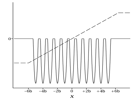
Figure 1. Plot of the multiple-wells potential $V_{N}$ (full line) and of the Stark-type potential $W_{N}$ (broken line), where $N=11$.  By $b>0$ we denote the distance between the adjacent absolute minima points.

The study of the dynamics of the wavefunction $\psi$, solution of (6), is then achieved by means of a discrete nonlinear Schrödinger equation (DNLS).  The idea is basically simple and it consists in assuming that the wavefunction $\psi$ may be written as a superposition of vectors $u_{\ell}(x)$ localized on the $\ell-$th cell of the lattice; that is

$$\psi(x,t)\sim\sum_{\ell=1}^{N}c_{\ell}(t)u_{\ell}(x)\,.$$

Such an approach has been successfully used in the cases of semiclassical NLS with multiple-well potentials [24] or with periodic potentials (see [14, 18, 19]), without the external field with potential $W_{N}$.  Eventually, $u_{\ell}(x)$ may coincide with the Wannier function $u_{\ell}^{W}(x)$ associated to the first band of the Bloch operator $H_{B}$ or with the semiclassical single well ground state eigenfunction $u_{\ell}^{sc}(x)$.  By means of such an approach the unknown functions $c_{\ell}(t)$ turn out to be the solutions of a system of time-dependent equations which dominant terms are given by (here we denote $\dot{}=\frac{d}{dt}$)

$$i\epsilon\dot{c}_{\ell}=-\lambda_{D}c_{\ell}-\beta\left(c_{\ell+1}+c_{\ell-1}\right)+\gamma\|u_{0}\|^{4}_{L^{4}}|c_{\ell}|^{2}c_{\ell}+fb\ell c_{\ell}\,,\ \ell=1,\ldots,N$$ (7)

where $\lambda_{D}$ is the ground state of a single cell potential and where $\beta$ is the hopping matrix element between neighboring sites.  In fact, the parameter $\beta$ is expected to be such that $4\beta$ is equal to the amplitude $B_{1}$ of the first band [25].  In (7) we’ll fix $c_{0}\equiv c_{N+1}\equiv 0$.  Equation (7) represents a discrete nonlinear Schrödinger equation (DNLS).

Our approach is both semiclassical and perturbative.  It is semiclassical in the sense that it holds true in the semiclassical regime of $\epsilon$ small enough; and it is perturbative in the sense that the external field $f$ and the nonlinearity power strength $\gamma$ must be small when $\epsilon$ goes to zero (see Hyp. 3 for details).  Under these conditions we prove the validity of the $N$-mode approximation (7) with a rigorous estimate of the remainder term for times of the order of the Bloch period.  Then, we numerically solve the $N$-mode approximation (7), and we compute the oscillating period taking into account the nonlinear interaction.  In fact, the behavior of the wavefunction is not simply periodic in time; it turns out that the center of mass $\langle x\rangle^{t}=\langle\psi,x\psi\rangle$ shows an oscillating motion with modulated amplitude.  The oscillating period turns out to be depending on the nonlinearity parameter strength $\gamma$ and we see that it also depends on the distribution of the initial wavefunction $\psi_{0}$.  In particular, when $\psi_{0}$ is a symmetric wavefunction then the oscillating period is almost constant for small $\gamma$ and it practically coincides with the Bloch period $T$; on the other hand when $\psi_{0}$ is an asymmetrical function the oscillating period actually depends on $\gamma$.  This fact is in contradiction with the Bloch Theorem (which holds true when $\gamma=0$), which implies that the Bloch period $T$ does not depend on the shape of the initial wavefunction, and it may explain the relatively large uncertainty observed by [20] in their experiments, as discussed in the Conclusions.

The paper is organized as follows.  In Section 2 we derive the DNLS (7) from the NLS (6) in the semiclassical limit $\epsilon\to 0$ for times of the order of the Bloch period $T$ with a rigorous estimate of the remainder term.  In particular: in §2.1 we introduce the assumptions and we recall some preparatory results; in §2.2 we derive the DNSL by making use of some ideas previously given by [24] and adapted to the case of multiple-well potential with an external Stark-type perturbation.  In Section 3 we consider a realistic experiment and we compute the wavefunction dynamics by making use of the DNLS.  In particular: in §3.1 we discuss the validity of the $N$-mode approximation for different values of the parameters; in §3.2 we numerically compute the wavefunction for times of the order of the Bloch period.  In Appendix we write the Wannier functions in terms of the Mathieu functions.

Notation

Let $g$ be a quantity depending on the semiclassical parameter $\epsilon$.  In the following

$$g=\tilde{\mathcal{O}}\left(e^{-S_{0}/\epsilon}\right)$$

means that for any $\epsilon^{\star}>0$ and any $\rho\in(0,S_{0})$ there exists $C:=C_{\rho,\epsilon^{\star}}$ such that

$$|g|\leq Ce^{-(S_{0}-\rho)/\epsilon}\,,\ \forall\epsilon\in(0,\epsilon^{\star})\,.$$

Hereafter, by $C$ we denote a generic positive constant independent of $\epsilon$.

Let $N\in{\mathbb{N}}$, then by ${\mathbb{N}}_{N}:=\{1,2,\ldots,N\}$ we denote the set of first $N$ positive integer numbers.

By $\|\cdot\|_{L^{p}}$ we denote the norm of the Banach space $L^{p}({\mathbb{R}})$, by $\langle\cdot,\cdot\rangle$ we denote the scalar product of the Hilbert space $L^{2}({\mathbb{R}})$.

2. Derivation of the DNLS (7)

2.1. Assumptions and preliminary results

We consider the time-dependent non-linear Schrödinger equation (6) where $V_{N}$ is a multiple-well potential and $W_{N}(x)$ is a bounded Stark-type potential.  In particular we assume that

Hypothesis 1.

Let $v(x)\in C_{0}^{\infty}({\mathbb{R}})$ be an even (i.e. $v(-x)=v(x)$) smooth function with compact support with a non degenerate minimum value at $x=0$:

$$v(x)>v_{min}=v(0),\ \forall x\in{\mathbb{R}}\,,\ x\not=0.$$

The multiple-well potential is defined as

$$V_{N}(x)=\sum_{\ell=1}^{N}v(x-x_{\ell})$$

for some fixed $N>1$, where $x_{\ell}=\left(\ell-\frac{N+1}{2}\right)b$ and where $b>0$ is such that $\mbox{supp}\ v\subset\left(-\frac{b}{2},+\frac{b}{2}\right)$.

Hence, by construction the potential $V_{N}(x)$ has exactly $N$ wells with not degenerate minima at $x=x_{\ell}$, $\ell\in{\mathbb{N}}_{N}$.

Remark 1.

We assume that $v(x)$ is an even function just for argument’s sake.  As discussed in Remark 6 this assumption may be removed.  Furthermore, we assume that $v$ is a smooth function as usual; in fact, a lessere regularity (e.g. $C^{2}$) would be enough.

Hypothesis 2.

Let $W_{N}(x)\in C({\mathbb{R}})$ be the monotone not decreasing function defined as

$$W_{N}(x)=\left\{\begin{array}[]{ll}-L&\mbox{ if }x<-L\\ x&\mbox{ if }x\in[-L,L]\\ L&\mbox{ if }x>L\end{array}\right.$$

for some $L>\frac{N+1}{2}b$.

That is the Stark-type potential $W_{N}$ is linear in the region containing the wells and it is a constant function outside this region (see Fig. 1).  In the “limit” where $N$ goes to infinity the potential $V_{N}$ becomes a periodic potential with period $b$ and the external potential $W_{N}$ becomes the Stark potential $x$.

Remark 2.

We restrict ourselves to a multiple-well potential $V_{N}$ with a finite number of wells only for sake of simplicity; one could consider the case of a periodic potential by making use of the tools developed by [14].  On the other side, the assumption on $W_{N}$ is not merely for the sake of simplicity; actually, the Stark-type potential $W_{N}$ is a bounded operator while the Stark potential $x$ is not a bounded operator and this fact is a source of several technical problems.  In fact, in real experiments the BEC are trapped in a finite spatial region.

Hypothesis 3.

We assume to be in the semiclassical limit, that is we look for the solution of (6) in the limit of $\epsilon$ that goes to zero.  We assume also that the other two parameters $\gamma$ and $f$ are small for $\epsilon$ small.  That is we assume that there exists $\epsilon^{\star}>0$ such that

$$Ce^{-(S_{0}-\rho)/\epsilon}\leq|f|\leq C\epsilon^{s}\,,\ \forall\epsilon\in(0,\epsilon^{\star})\,,$$

for some $s>2$, $C>0$ and $\rho\in(0,S_{0})$ independent of $\epsilon$; furthermore, we assume also that

$$\frac{|\gamma|\epsilon^{-1/2}}{|f|}\leq C$$ (9)

for some positive constant $C$ and for any $\epsilon\in(0,\epsilon^{\star})$.

The self-adjoint extension of the linear Schrödinger operator formally defined on $L^{2}({\mathbb{R}})$ as

$$H_{N}=-\epsilon^{2}\partial^{2}_{xx}+V_{N}$$

has an almost degenerate ground state with dimension $N$.  More precisely, let $\lambda_{\ell}$, $\ell\in{\mathbb{N}}_{N}$, be the lowest eigenvalues of $H_{N}$ with associated normalized eigenvectors $v_{\ell}$.  In particular we have that (see Lemma 2 [25])

$$\lambda_{\ell}=\lambda_{D}-2\beta\cos\left(\ell\frac{\pi}{N+1}\right)+O(\epsilon^{\infty})e^{-S_{0}/\epsilon}\,,\ \ell\in{\mathbb{N}}_{N}\,,$$

where

$$S_{0}=\int_{x_{0}}^{x_{1}}\sqrt{V_{N}(x)-v_{min}}\,dx>0$$

is the Agmon distance between two wells and $\lambda_{D}$ is the ground state of the single well operator $-\epsilon^{2}\partial_{xx}^{2}+v$, where the single well potential $v$ has been introduced by Hyp. 1.  The numerical pre-factor $\beta$ is the hopping matrix element between neighboring wells, and it is such that $4\beta$ is asymptotic to the amplitude of the first band of the periodic Bloch operator $H_{B}$; i.e. $4\beta\sim B_{1}:=E_{1}^{t}-E_{1}^{b}$ where $E_{1}^{b}$ and $E_{1}^{t}$ are, respectively, the bottom and the top of the first band.  Such a numerical pre-factor is going to be exponentially small, i.e.

$$\beta={\tilde{\mathcal{O}}}(e^{-S_{0}/\epsilon})\ \mbox{ as }\ \epsilon\to 0^{+}\,.$$

Remark 3.

Hyp. 3 means that, from a practical point of view, the parameter $f$ cannot be arbitrarily small, but it has a lower bound of order $\beta$.  On the other hand, the parameter $\gamma$ may be arbitrarily small.

The associated normalized eigenvectors are given by [25]

$$v_{\ell}=\sum_{j=1}^{N}\alpha_{\ell,j}u_{j}^{sc}+O(\epsilon^{\infty})e^{-S_{0}/\epsilon}$$

where

$$\alpha_{j,\ell}=\alpha_{\ell,j}=\sqrt{\frac{2}{N+1}}\sin\left(j\ell\frac{\pi}{N+1}\right)$$

and where $u_{j}^{sc}(x)$ is the semiclassical single well ground state eigenfunction localized on the $j$-th cell; by construction and since $v(x)$ is an even function then

$$u_{j}^{sc}(x)=u_{0}^{sc}(x-x_{j})\ \mbox{ and }\ u_{0}^{sc}(x)=u_{0}^{sc}(-x)\,.$$ (10)

Now, let $\Pi$ be the projection operator associated with the $N$ eigenvalues $\lambda_{\ell}$, i.e.

$$\Pi=\sum_{\ell=1}^{N}\langle v_{\ell},\cdot\rangle v_{\ell}$$

and let

$$\Pi_{c}=1-\Pi\,.$$

Let $F=\Pi(L^{2}({\mathbb{R}}))$ be the $N$-dimensional space spanned by the $N$ eigenvectors $v_{\ell}$, $\ell\in{\mathbb{N}}_{N}$.

Remark 4.

Let $\sigma(H_{N})$ be the spectrum of $H_{N}$; then it is a well known semiclassical result that

$$C^{-1}\epsilon\leq\mbox{\rm dist}\left(\left\{\lambda_{\ell}\right\}_{\ell=1}^{N},\sigma(H_{N})\setminus\left\{\lambda_{\ell}\right\}_{\ell=1}^{N}\right)\leq C\epsilon$$

for some positive constant $C>0$.  Hence, since $H_{N}$ is a self-adjoint operator then

$$\left\|[H_{N}-\lambda_{D}]^{-1}\Pi_{c}\right\|_{{\mathcal{L}}(L^{2}\to L^{2})}\leq C\epsilon^{-1}$$

for some $C>0$.

Remark 5.

By [14] it has been proved that there exists a suitable orthonormal base $u_{\ell}$, $\ell\in{\mathbb{N}}_{N}$, of the space $F$.  The functions $u_{\ell}$ are practically localized on the $\ell$-th well.  More precisely, they are such that

• $\|u_{\ell}-u_{\ell}^{sc}\|_{L^{p}}=\tilde{\mathcal{O}}\left(e^{-S_{0}/\epsilon}\right)$ for any $p\in[2,+\infty]$ and any $\ell\in{\mathbb{N}}_{N}$;

• $\|u_{\ell}u_{j}\|_{L^{1}}=\tilde{\mathcal{O}}\left(e^{-S_{0}|j-\ell|/\epsilon}\right)$ for any $j,\ell\in{\mathbb{N}}_{N}$;

• $\|u_{\ell}\|_{L^{p}}\leq C\epsilon^{-\frac{p-2}{4p}}$, $p\in[2,+\infty]$, and $\|\partial_{x}u_{\ell}\|_{L^{2}}\leq C\epsilon^{-1/2}$ for any $\ell\in{\mathbb{N}}_{N}$;

• The matrix with elements $\langle u_{\ell},H_{N}u_{j}\rangle$ can be written as

  $$\left(\langle u_{\ell},H_{N}u_{j}\rangle\right)=\lambda_{D}\mbox{\sc 1}_{N}-\beta{\mathcal{T}}+D_{N}$$

  where ${\mathcal{T}}$ is the tridiagonal Toeplix matrix such that

  $${\mathcal{T}}_{j,\ell}=\left\{\begin{array}[]{ll}0&\mbox{ if }\ |j-\ell|\not=1\\ 1&\mbox{ if }\ |j-\ell|=1\end{array}\right.$$

  and where the remainder term $D_{N}$ is a bounded linear operator from $\ell^{p}({\mathbb{N}}_{N})$ to $\ell^{p}({\mathbb{N}}_{N})$ with bound

  $$\|D_{N}\|_{{\mathcal{L}}(\ell^{p}({\mathbb{N}}_{N})\to\ell^{p}({\mathbb{N}}_{N}))}=\tilde{\mathcal{O}}\left(e^{-(S_{0}+\alpha)/\epsilon}\right)\,,\ p\in[1,+\infty]\,,$$

  for some $\alpha>0$.

We finally assume that the initial state is prepared on the first $N$ “ground states”.  That is

Hypothesis 4.

$\Pi_{c}\psi_{0}=0$.

It is well known that under the assumptions above the NLS (6) is locally well posed, and the conservation of the norm and of the energy [6, 7]

$${\mathcal{E}}(\psi)=\langle\psi,H_{N}\psi\rangle+\frac{1}{2}\gamma\|\psi\|_{L^{4}}^{4}+f\langle\psi,W_{N}\psi\rangle$$

easily follow:

$$\|\psi(\cdot,t)\|_{L^{2}}=\|\psi_{0}(\cdot)\|_{L^{2}}\ \mbox{ and }\ {\mathcal{E}}\left(\psi(\cdot,t)\right)={\mathcal{E}}\left(\psi_{0}(\cdot)\right)\,.$$

Furthermore the following a priori estimate follows, too.

Lemma 1.

There exists a positive constant $C>0$ such that

$$\|\psi\|_{H^{1}}\leq C\epsilon^{-1/2}\ \mbox{ and }\ \|\psi\|_{L^{p}}^{p}\leq C\epsilon^{-\frac{p-2}{4}}\,,\forall p\in[2,+\infty]\,.$$

Proof.

Indeed, from Theorem 2 by [24] and its remarks it follows that

$$\|\nabla\psi\|_{L^{2}}\leq C\sqrt{\Lambda}\ \mbox{ and }\ \|\psi\|_{L^{p}}\leq C\Lambda^{\frac{p-2}{4p}}$$

for some $C>0$ and $\epsilon$ small enough, where

$$\Lambda=\frac{\mathcal{E}(\psi_{0})-V_{min}}{\epsilon^{2}}$$

and where $V_{min}=\min_{x}[V_{N}(x)+fW_{N}(x)]$.  In particular, since $fW_{N}(x)\geq-fL=O(\epsilon^{s})$ for some $s>2$, because $L$ is fixed, and since $\Pi_{c}\psi_{0}=0$ then $\Lambda\sim\epsilon^{-1}$; therefore

$$\|\nabla\psi\|_{L^{2}}\leq C\epsilon^{-1/2}\ \mbox{ and }\ \|\psi\|_{L^{p}}\leq C\epsilon^{-\frac{p-2}{4p}}\,.$$

∎

Hence, the global well-posedness of the NLS follows [6, 7].

2.2. N-mode approximation

Let $\psi$ be the normalized solution of the NLS equation written in the formula

$$\psi=\psi_{1}+\psi_{c}\,,\ \psi_{1}=\Pi\psi=\sum_{\ell=1}^{N}c_{\ell}u_{\ell}\ \mbox{ and }\ \psi_{c}=\Pi_{c}\psi\,,$$ (12)

for some complex-valued functions $c_{\ell}(t)$.  By substituting (12) into the NLS (6) then it takes the formula

$$\left\{\begin{array}[]{ll}i\epsilon\partial_{t}c_{\ell}=\langle u_{\ell},H_{N}\psi_{1}\rangle+\gamma\langle u_{\ell},|\psi(\cdot,\tau)|^{2}\psi(\cdot,\tau)\rangle+f\langle u_{\ell},W_{N}\psi(\cdot,\tau)\rangle\\ i\epsilon\partial_{t}\psi_{c}=H_{N}\psi_{c}+\gamma\Pi_{c}|\psi(\cdot,\tau)|^{2}\psi(\cdot,\tau)+f\Pi_{c}W_{N}\psi(\cdot,\tau)\end{array}\right.$$ (15)

We are going now to get an a priori estimate of the remainder term $\psi_{c}$.  First of all we rescale the time $t\to\tau=\frac{\beta}{\epsilon}t$ and we redefine the wavefunction up to a gauge factor $\psi(x,t)\to\psi(x,\tau):=e^{-i\lambda_{D}t/\epsilon}\psi(x,t)$.  The Bloch period becomes

$$\tau_{B}=\frac{\beta}{\epsilon}T=\frac{2\pi\beta}{|f|b}$$

Hence, (15) becomes (where ^′ denotes the derivative with respect to $\tau$)

$$\left\{\begin{array}[]{ll}i\beta c_{\ell}^{\prime}=\langle u_{\ell},(H_{N}-\lambda_{D})\psi_{1}\rangle+\gamma\langle u_{\ell},|\psi(\cdot,t)|^{2}\psi(\cdot,t)\rangle+f\langle u_{\ell},W_{N}\psi(\cdot,t)\rangle\\ i\beta\psi_{c}^{\prime}=(H_{N}-\lambda_{D})\psi_{c}+\gamma\Pi_{c}|\psi(\cdot,t)|^{2}\psi(\cdot,t)+f\Pi_{c}W_{N}\psi(\cdot,t)\end{array}\right.$$ (18)

Theorem 1.

Let Hyp.1-4 be satisfied; then it follows that the remainder $\psi_{c}$ can be estimated for times of order of the Bloch period.  That is for any fixed $M\in{\mathbb{N}}$ it follows that

$$\max_{\tau\in[0,M\tau_{B}]}\|\psi_{c}(\cdot,\tau)\|_{L^{2}}\leq C\frac{|f|}{\epsilon}$$

for some positive constant $C>0$.

Proof.

From the first equation of (18) and recalling that

$$\sum_{\ell=1}^{N}|c_{\ell}(\tau)|^{2}=\|\psi_{1}\|_{L^{2}}^{2}=1-\|\psi_{c}\|_{L^{2}}^{2}\leq 1$$

then a priori estimate follows

$$|c_{\ell}^{\prime}| \leq \frac{\langle u_{\ell},(H_{N}-\lambda_{D})\psi_{1}\rangle}{\beta}+\frac{|\gamma|}{\beta}\|\psi\|_{L^{\infty}}^{2}+\frac{|f|}{\beta}\|W_{N}\|_{L^{\infty}}$$ (19)

$$\leq C+\frac{|\gamma|\epsilon^{-1/2}}{\beta}+\frac{|f|}{\beta}L$$

because $\|u_{\ell}\|_{L^{2}}=1$ and $\|\psi\|_{L^{2}}=1$, and from Remark 5 iv. and Lemma 1.

Concerning $\psi_{c}$ it satisfies to the following integral equation

$$\psi_{c}=I+II$$

where we set

$$I := -\frac{i}{\beta}\int_{0}^{\tau}e^{-i(H_{N}-\lambda_{D})(\tau-s)/\beta}\Pi_{c}Ads$$

$$II := -\frac{i}{\beta}\int_{0}^{\tau}e^{-i(H_{N}-\lambda_{D})(\tau-s)/\beta}\Pi_{c}Bds$$

and where $A$ and $B$ are defined as

$$A := \gamma|\psi_{1}|^{2}\psi_{1}+fW_{N}\psi_{1}$$

$$B := \gamma\left[\bar{\psi}_{1}\psi_{c}^{2}+|\psi_{c}|^{2}\psi_{c}+2|\psi_{1}|^{2}\psi_{c}+2|\psi_{c}|^{2}\psi_{1}+\psi_{1}^{2}\bar{\psi}_{c}\right]+fW_{N}\psi_{c}$$

such that

$$A+B=\gamma|\psi|^{2}\psi+fW_{N}\psi\,.$$

By means of standard arguments [24] and making use of the fact that the operator $W_{N}$ is bounded then it follows that

Lemma 2.

Let

$$\Gamma=|\gamma|\epsilon^{-1/2}+|f|\,.$$

Then the functions $A$ and $B$ are such that

$$\|A\|_{L^{2}}\leq C\Gamma\,,\ \|B\|_{L^{2}}\leq C\Gamma\|\psi_{c}\|_{L^{2}}\ \mbox{ and }\ \left\|\frac{\partial A}{\partial\tau}\right\|_{L^{2}}\leq C\Gamma^{2}\beta^{-1}\,.$$

Proof.

Indeed,

$$\|A\|_{L^{2}}\leq|\gamma|\,\|\psi_{1}\|_{L^{\infty}}^{2}\|\psi_{1}\|_{L^{2}}+|f|\|W_{N}\|_{L^{\infty}}\|\psi_{1}\|_{L^{2}}\leq C\left[|\gamma|\epsilon^{-1/2}+|f|\right]$$

since $\|\psi_{1}\|_{L^{\infty}}\leq C\max_{\ell}\|u_{\ell}\|_{L^{\infty}}\leq C\epsilon^{-1/4}$.  Similarly, the estimate of the function $B$ follows recalling that $\|\psi_{c}\|_{L^{\infty}}\leq C\epsilon^{-1/4}$ from Lemma 1.  Finally, the estimate concerning $\frac{\partial A}{\partial\tau}$ immediately follows from (19). ∎

Hence, the estimates of the integrals I and II follow; in particular, integral II can be simply estimated as

$$\|II\|_{L^{2}}\leq C\Gamma\beta^{-1}\int_{0}^{\tau}\|\psi_{c}(\cdot,s)\|_{L^{2}}ds$$

since

$$\left\|e^{-i(H_{N}-\lambda_{D})(\tau-s)/\beta}\right\|_{{\mathcal{L}}(L^{2}\to L^{2})}=1\,.$$

On the other hand, before to get the estimate of integral I we perform an integration by parts in order to gain a pre-factor $\beta$:

$$I = \left[-ie^{-i(H_{N}-\lambda_{D})(\tau-s)/\beta}[H_{N}-\lambda_{D}]^{-1}\Pi_{c}A\right]_{0}^{\tau}+$$

$$\ \ +i\int_{0}^{\tau}e^{-i(H_{N}-\lambda_{D})(\tau-s)/\beta}[H_{N}-\lambda_{D}]^{-1}\Pi_{c}\frac{\partial A}{\partial s}ds$$

From this fact and recalling that (Remark 4)

$$\|[H_{N}-\lambda_{D}]^{-1}\Pi_{c}\|_{{\mathcal{L}}(L^{2}\to L^{2})}\leq C\epsilon^{-1}$$

then

$$\|I\|_{L^{2}}\leq C\epsilon^{-1}\max_{s\in[0,\tau]}\left[\|A\|_{L^{2}}+\tau\left\|\frac{\partial A}{\partial s}\right\|_{L^{2}}\right]\leq C\epsilon^{-1}\Gamma[1+\Gamma\beta^{-1}\tau]\,.$$

Therefore, we have that

$$\|\psi_{c}\|_{L^{2}}\leq C\Gamma\beta^{-1}\int_{0}^{\tau}\|\psi_{c}(\cdot,s)\|_{L^{2}}\,ds+C\epsilon^{-1}\Gamma(1+\Gamma\beta^{-1}\tau)\,.$$

From the Gronwall’s Lemma it follows that

$$\|\psi(\cdot,\tau)\|_{L^{2}}\leq C\epsilon^{-1}\Gamma(1+\Gamma\beta^{-1}\tau)e^{C\Gamma\beta^{-1}\tau}$$

In particular we observe that

$$\max_{\tau\in[0,M\tau_{B}]}\|\psi(\cdot,\tau)\|_{L^{2}}\leq C\epsilon^{-1}\Gamma(1+\beta^{-1}\Gamma M\tau_{B})e^{C\Gamma\beta^{-1}M\tau_{B}}\leq C\Gamma\epsilon^{-1}\leq C\frac{|f|}{\epsilon}$$

proving the Theorem since $\Gamma\leq C|f|$ from Hyp. 3 and since $\tau_{B}=\frac{2\pi}{b}\frac{\beta}{|f|}$. ∎

We are going now to estimate the solutions $c_{\ell}$ of the first equation of (18) which can be written as

$$i\beta c_{\ell}^{\prime}=\langle u_{\ell},(H_{N}-\lambda_{D})\psi_{1}\rangle+\langle u_{\ell},A\rangle+\langle u_{\ell},B\rangle$$

where the term $\langle u_{\ell},(H_{N}-\lambda_{D})\psi_{1}\rangle$ can be represented by property iv. of Remark 5.  Concerning the term $\langle u_{\ell},B\rangle$ the following estimate uniformly holds with respect to the index $\ell$

$$\left|\langle u_{\ell},B\rangle\right|\leq\|B\|_{L^{2}}\leq C\Gamma\|\psi_{c}\|_{L^{2}}\,.$$

Furthermore

$$\langle u_{\ell},A\rangle = \gamma\sum_{j,k,m=1}^{N}\bar{c}_{j}c_{k}c_{m}\langle u_{\ell},\bar{u}_{j}u_{k}u_{m}\rangle+f\sum_{j=1}^{N}c_{j}\langle u_{\ell},W_{N}u_{j}\rangle$$

$$= \gamma|c_{\ell}|^{2}c_{\ell}\|u_{\ell}\|_{L^{4}}^{4}+fc_{\ell}\langle u_{\ell},W_{N}u_{\ell}\rangle+\gamma r_{\ell}^{a}+fr_{\ell}^{b}$$

where

$$r_{\ell}^{a}=\sum_{j,k,m\in{\mathbb{N}}_{N}\ :\ |j-\ell|+|m-\ell|+|k-\ell|>0}\bar{c}_{j}c_{k}c_{m}\langle u_{\ell},\bar{u}_{j}u_{k}u_{m}\rangle$$

and

$$r_{\ell}^{b}=\sum_{j,\ell\in{\mathbb{N}}_{N}\,,\ j\not=\ell}c_{j}\langle u_{\ell},W_{N}u_{j}\rangle$$

are remainder terms.

We have that

Lemma 3.

The following estimates uniformly hold with respect to the indexes $\ell\,,\ j\,,\ m$ and $k$:

• $\langle u_{\ell},W_{N}u_{\ell}\rangle=\ell b+\tilde{\mathcal{O}}\left(e^{-S_{0}/\epsilon}\right)$;

• $\langle u_{\ell},W_{N}u_{j}\rangle=\tilde{\mathcal{O}}\left(e^{-S_{0}|j-\ell|/\epsilon}\right)$;

• $\langle u_{\ell},\bar{u}_{j}u_{m}u_{k}\rangle=\tilde{\mathcal{O}}\left(e^{-S_{0}r/\epsilon}\right)$ where

  $$r=\max\left[|j-\ell|,|m-\ell|,|k-\ell|,|j-m|,|j-k|,|k-m|\right].$$

Proof.

Indeed, let $I_{\ell}=\left[x_{\ell}-b,x_{\ell}+b\right]$, then

$$\langle u_{\ell},W_{N}u_{\ell}\rangle=\int_{I_{\ell}}|u_{\ell}(x)|^{2}xdx+\int_{{\mathbb{R}}\setminus I_{\ell}}|u_{\ell}(x)|^{2}W_{N}(x)dx$$

where $u_{\ell}(x)=u_{0}(x-x_{\ell})+\tilde{\mathcal{O}}\left(e^{-S_{0}/\epsilon}\right)$ from (10) and Remark 4.  Therefore

$$\int_{I_{\ell}}|u_{\ell}(x)|^{2}xdx = \ell b\int_{I_{0}}|u_{0}(x)|^{2}dx+\int_{I_{0}}|u_{0}(x)|^{2}xdx+\tilde{\mathcal{O}}\left(e^{-S_{0}/\epsilon}\right)$$

$$= \ell b\left[\|u_{0}\|^{2}_{L^{2}}-\|u_{0}\|^{2}_{L^{2}({\mathbb{R}}\setminus I_{0})}\right]+\tilde{\mathcal{O}}\left(e^{-S_{0}/\epsilon}\right)$$

where $u_{0}$ is normalized and $\int_{I_{0}}|u_{0}(x)|^{2}xdx=\tilde{\mathcal{O}}\left(e^{-S_{0}/\epsilon}\right)$ because $u_{0}(x)=u_{0}(-x)+\tilde{\mathcal{O}}\left(e^{-S_{0}/\epsilon}\right)$.  From this fact and since $\|u_{\ell}\|_{L^{2}({\mathbb{R}}\setminus I_{\ell})}=\tilde{\mathcal{O}}(e^{-S_{0}/\hbar})$ (see Lemma 4 iii. and Lemma 5 by [14]) then the asymptotic behavior i. follows.  The other two asymptotic behaviors ii. and iii. similarly follow from property ii. by Remark 5; indeed

$$|\langle u_{\ell},W_{N}u_{j}\rangle|\leq\|W_{N}\|_{L^{\infty}}\|u_{\ell}u_{j}\|_{L^{1}}=\tilde{\mathcal{O}}\left(e^{-S_{0}|j-\ell|/\epsilon}\right)$$

and, where we assume that $r=|j-\ell|$,

$$|\langle u_{\ell},\bar{u}_{j}u_{m}u_{k}\rangle|\leq\|u_{m}\|_{L^{\infty}}\|u\|_{L^{\infty}}\|u_{\ell}u_{j}\|_{L^{1}}=\tilde{\mathcal{O}}\left(e^{-S_{0}r/\epsilon}\right)$$

proving so the estimates ii. and iii.. ∎

From this Lemma and from the previous computation it follows that the first equation of (18) becomes a DNLS of the form

$$i\beta c_{\ell}^{\prime}=-\beta\sum_{m=1}^{N}{\mathcal{T}}_{\ell,m}c_{m}+\gamma\|u_{\ell}\|_{L^{4}}^{4}|c_{\ell}|^{2}c_{\ell}+f\ell bc_{\ell}+\tilde{\mathcal{O}}\left(e^{-S_{0}/\epsilon}\right)$$ (20)

where

$$\|u_{\ell}\|_{L^{4}}^{4}=\|u_{0}\|_{L^{4}}^{4}+\tilde{\mathcal{O}}\left(e^{-S_{0}/\epsilon}\right)$$

and where the remainder terms $\tilde{\mathcal{O}}\left(e^{-S_{0}/\epsilon}\right)$ are uniform with respect to the index $\ell$.

Remark 6.

In fact, if $v(x)$ is not an even function then by means of standard semiclassical arguments it follows that property Lemma 3 i. becomes

$$\langle u_{\ell},W_{N}u_{\ell}\rangle=\ell b+c+\tilde{\mathcal{O}}\left(e^{-S_{0}/\epsilon}\right)$$

for some constant $c$ independent of the index $\ell$.  In such a case we must add the term $fcc_{\ell}$ to the right hand side of the DNLS above and, by means of a gauge choice $c_{\ell}\to c_{\ell}e^{-i\frac{fc}{\beta}\tau}$, we can remove this term obtaining again equation (20).

Now, we are able to prove that

Theorem 2.

Let $d_{\ell}(\tau)$ be the solutions of the DNLS

$$i\beta d_{\ell}^{\prime}=-\beta\sum_{m=1}^{N}{\mathcal{T}}_{\ell,m}d_{m}+\gamma\|u_{0}^{sc}\|_{L^{4}}^{4}|d_{\ell}|^{2}d_{\ell}+f\ell bd_{\ell}$$ (21)

satisfying to the initial conditions $d_{\ell}(0)=c_{\ell}(0)$, where $c_{\ell}(\tau)$ and $\psi_{c}$ are the solutions of (18).  Then, for any fixed $M\in{\mathbb{N}}$ it follows that

$$\max_{\tau\in[0,M\tau_{B}],\,\ell=1,2,\ldots,N}|c_{\ell}(\tau)-d_{\ell}(\tau)|=\tilde{\mathcal{O}}\left(e^{-S_{0}/\epsilon}\right)\ \mbox{ as }\ \epsilon\to 0\,.$$

Proof.

The proof is a simply consequence of equation (20) and from the fact that $\tau_{B}=\frac{2\pi}{b}\frac{\beta}{f}$ and Hyp.3. ∎

3. Numerical analysis of a real model

We consider the experiment where a cloud of ultracold Strontium atoms ${}^{88}Sr$ are trapped in a one-dimensional optical lattice with potential (2).  Realistic data for the experiment are [20]:

• Lattice period: $b=\lambda_{L}/2=266\,nm$, $\lambda_{L}=532\,nm$;

• Lattice potential depth: $V_{0}=\Lambda_{0}\cdot E_{R}$ where $E_{R}$ is the photon recoil energy $E_{R}=\frac{2\pi^{2}\hbar^{2}}{m\lambda_{L}^{2}}=50.38\,kHz\cdot\hbar$ and where $\Lambda_{0}$ is between $3$ and $10$;

• Mass of the strontium $88$ isotope: $m=87.91\,au=1.46\cdot 10^{-22}\,gr$;

• Effective one-dimensional nonlinearity strength: let $\gamma_{3D}=\frac{4{\mathcal{N}}\pi a_{s}\hbar^{2}}{m}$ be the effective nonlinearity strength for the three-dimensional Gross-Pitaevskii equation, then it is expected that the effective one-dimensional nonlinearity strength $\gamma$ is of the order [26]

  $$\gamma\approx\frac{\gamma_{3D}}{2\pi d_{\perp}^{2}}$$

  where $d_{\perp}$ is the oscillator length of the transverse confinement; here $a_{s}$ denotes the scattering length of the Strontium $88$ isotope: $a_{s}=-a_{0}\div 13a_{0}$, where $a_{0}$ is the Bohr radius; ${\mathcal{N}}$ is the number of atoms of the condensate; in typical experiments $d_{\perp}\approx 180\cdot 10^{-6}\,m$ and ${\mathcal{N}}=10^{5}\div 10^{6}$;

• Acceleration constant $g=9.807\,m/s^{2}$.

The confined BEC is governed by Eq. (6) and here we make use of the $N$-mode approximation (21), that is the wavefunction $\psi$ has the form $\psi\sim\sum_{\ell}c_{\ell}u_{\ell}$ where $c_{\ell}$ are the solutions of (21) and where $u_{\ell}$ are functions localized on the $\ell$-th lattice site.  In order to justify the validity of such an approximation we’ll check if the model is in the semiclassical regime, that is if the first band is almost flat and if semi-classical approximation $u_{\ell}^{sc}$ agrees or not with the Wannier function $u_{\ell}^{W}$.  Such a qualitative criterion has been also adopted by other authors [2, 3, 11] and we’ll see that our results agree with the results contained in these papers.  In particular, in [11] has been computed the hopping matrix elements $\langle u_{\ell},H_{N}u_{j}\rangle$ too, where it has been numerically verified that these coefficients are negligible when $|j-\ell|>1$ for $\Lambda_{0}\geq 10$; thus, for such values of $\Lambda_{0}$ it is admitted that the $N$-mode approximation, consisting to describe (6) in terms of a nearest-neighbor model (21), works.

3.1. Validity of the semiclassical approximation

The semiclassical approximation $u_{0}^{sc}(x)$ of the wavefunction has dominant behavior

$$u_{0}^{sc}(x)=\frac{(m\mu)^{1/8}}{(\pi\hbar)^{1/4}}e^{-\sqrt{m\mu}x^{2}/2\hbar}$$ (22)

in the semiclassical limit, where $\mu=\frac{d^{2}V_{per}(0)}{dx^{2}}=2V_{0}k_{L}^{2}$, $V_{0}=\Lambda_{0}E_{R}$; it is normalized $\|u_{0}^{sc}\|_{L^{2}}=1$.  We may remark that the effective semiclassical parameter in adimensional units is given by

$$\frac{1}{\sqrt{\Lambda_{0}}}=\frac{2\pi^{2}\hbar}{b^{2}\sqrt{m\mu}}\,,$$

and then the semiclassical approximation may be written as

$$u_{0}^{sc}(x)=\left[\frac{2\pi\sqrt{\Lambda_{0}}}{b^{2}}\right]^{1/4}e^{-x^{2}\pi^{2}\sqrt{\Lambda_{0}}/b^{2}}\,.$$

Hence

$$\|u_{0}^{sc}\|_{L^{4}}^{4}=\left[\frac{m\mu}{(\pi\hbar)^{2}}\right]^{1/4}\sqrt{\frac{\pi}{2}}=\frac{\pi\Lambda_{0}^{1/4}}{b}.$$

We’ll see that for $\Lambda_{0}$ “large enough” (i.e. $\Lambda_{0}\geq 10$) then the first band is almost flat and the semiclassical function $u_{0}^{sc}$ well approximates the Wannier function $u_{0}^{W}$, as we expect to observe in the semiclassical limit $\Lambda_{0}\to\infty$ (see, e.g., [30]).

Remark 7.

By the scaling

$$x\to 2k_{L}x\,,\ t\to E_{R}t/\hbar\,,\psi(x)\to\frac{1}{\sqrt{2k_{L}}}\psi\left(\frac{x}{2k_{L}}\right)$$

and setting

$$F=\frac{mg}{2E_{R}k_{L}}\,,\ \zeta=\frac{\gamma}{2E_{R}k_{L}}\,,\ \epsilon=\frac{1}{\sqrt{\Lambda_{0}}}$$

then (3) takes the form

$$i\partial_{t}\psi=-\partial^{2}_{xx}\psi+\frac{1}{\epsilon^{2}}\sin^{2}(x/2)+Fx\psi+\zeta|\psi|^{2}\psi\,,\ \|\psi\|_{L^{2}}=1\,.$$ (23)

Equation (23) is equivalent, up to a change of scale of the time, to the equation

$$i\epsilon\partial_{t}\psi=-\epsilon^{2}\partial^{2}_{xx}\psi+\sin^{2}\left(\frac{x}{2}\right)\psi+fx\psi+\gamma|\psi|^{2}\psi$$

where we set

$$t\to t/\sqrt{\epsilon}\,,\ f=F\epsilon^{2}\,,\ \gamma=\epsilon^{2}\zeta\,.$$

and where $\epsilon=\Lambda_{0}^{-1/2}$ plays the role of the semiclassical parameter.

We compute now the band functions and the Wannier functions for different values of $\Lambda_{0}$.  The semiclassical wavefunction $u_{0}^{sc}$ is computed by (22), while the Wannier function $u_{0}^{W}(x)$ may be computed by means of the Mathieu functions (see Appendix).

3.1.1. Model $\Lambda_{0}=3$

The first bands of the Bloch operator $H_{B}=-\frac{\hbar^{2}}{2m}\partial^{2}_{xx}+\Lambda_{0}E_{R}\sin^{2}(k_{L}x)$ have endpoints

• ${E}_{1}^{b}=1.43\cdot E_{R}$ and ${E}_{1}^{t}=2.11\cdot E_{R}$;

• ${E}_{2}^{b}=2.86\cdot E_{R}$ and ${E}_{2}^{t}=5.49\cdot E_{R}$;

• ${E}_{3}^{b}=5.56\cdot E_{R}$ and ${E}_{3}^{t}=10.51\cdot E_{R}$.

Hence, the values of the width of the first two bands are given by

$$B_{1}:={E}_{1}^{t}-{E}_{1}^{b}=0.68\cdot E_{R}\ \ \mbox{ and }\ \ B_{2}:={E}_{2}^{b}-{E}_{1}^{t}=2.63\cdot E_{R}\,.$$

Furthermore it follows that the first gap has amplitude $g_{1}=E_{2}^{b}-E_{1}^{t}=0.77\cdot E_{R}$ of the order of the first band amplitude, while the width of the other gaps are very small (see Fig. 2, left hand side panel).  If we compare the first Wannier function $u_{0}^{W}(x)$ and the semiclassical approximation $u_{0}^{sc}(x)$ it turns out that (see also Fig. 2, right hand side panel)

$$\|u_{0}^{W}-u_{0}^{sc}\|_{L^{2}}^{2}=0.091$$

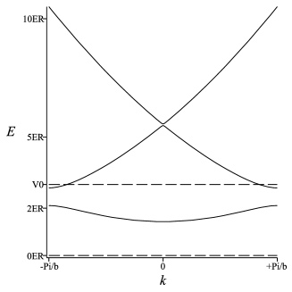
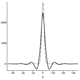
Figure 2. Here we plot in the left hand side panel the first three band functions $E_{n}(k)$, $n=1,2,3$ and $k\in\left[-\frac{\pi}{b},+\frac{\pi}{b}\right]$, for the Bloch operator $H_{B}$ where $\Lambda_{0}=3$.  It turns out that the width of the first gap is of the same order of the width of the first band.  In the right hand side panel we plot the graph of the functions $u_{0}^{sc}$ (broken line) and $u_{0}^{W}$ (full line).

3.1.2. Model $\Lambda_{0}=10$

The first bands of the Bloch operator $H_{B}$ have endpoints

• ${E}_{1}^{b}=4.32\cdot E_{R}$ and ${E}_{1}^{t}=4.58\cdot E_{R}$;

• ${E}_{2}^{b}=7.02\cdot E_{R}$ and ${E}_{2}^{t}=8.87\cdot E_{R}$;

• ${E}_{3}^{b}=9.54\cdot E_{R}$ and ${E}_{3}^{t}=14.07\cdot E_{R}$.

Hence, the values of the width of the first two bands are given by

$$B_{1}:={E}_{1}^{t}-{E}_{1}^{b}=0.26\cdot E_{R}\ \ \mbox{ and }\ \ B_{2}:={E}_{2}^{b}-{E}_{1}^{t}=1.85\cdot E_{R}\,.$$

Furthermore it also follows that the first gap has amplitude $g_{1}=E^{b}_{2}-E_{1}^{t}=2.44\cdot E_{R}$ is much larger than the amplitude of the first band and that the width of the other gaps are very small (see Fig. 3, left hand side panel).  If we compare the first Wannier function $u^{W}_{0}(x)$ and the semiclassical approximation $u_{0}^{sc}(x)$ it turns out that (see also Fig. 3, right hand side panel)

$$\|u_{0}^{W}-u_{0}^{sc}\|_{L^{2}}^{2}=0.055\,.$$

Hence, we may conclude that for $\Lambda_{0}=10$ the $N$-mode approximation properly works.

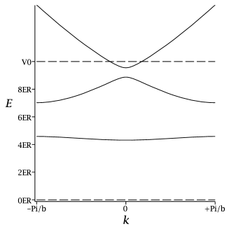
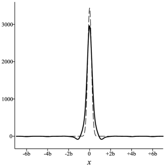
Figure 3. Here we plot in the left hand side panel the first three band functions $E_{n}(k)$, $n=1,2,3$ and $k\in\left[-\frac{\pi}{b},+\frac{\pi}{b}\right]$, for the Bloch operator $H_{B}$ where $\Lambda_{0}=10$.  It turns out that the first band is almost flat, in fact its width is $1/10$-th of the width of the first gap.  In the right hand side panel we plot the graph of the functions $u_{0}^{sc}$ (broken line) and $u_{0}^{W}$ (full line).

3.2. Numerical analysis of the model for $\Lambda_{0}=10$

We have seen that for $\Lambda_{0}\geq 10$ the $N$-mode approximation is justified.  For $\Lambda_{0}=10$ we have that

$$\beta\sim\frac{1}{4}B_{1}=0.065\cdot E_{R}\,.$$

Equation (21) takes the form

$$id_{\ell}^{\prime}=-\sum_{m=1}^{N}{\mathcal{T}}_{\ell,m}d_{m}+\eta|d_{\ell}|^{2}d_{\ell}+\ell\delta d_{\ell}\,,\ \ell\in{\mathbb{N}}_{N}\,,$$

where we set

$$\eta=\frac{\gamma\|u_{0}^{sc}\|_{L^{4}}^{4}}{\beta}\approx\frac{4{\mathcal{N}}\pi a_{s}\hbar^{2}}{m}\frac{{\pi}\Lambda_{0}^{1/4}}{b}\frac{1}{2\pi d_{\perp}^{2}}\frac{1}{\beta}=-0.151\cdot 10^{-1}\div 0.197$$

and

$$\delta=\frac{fb}{\beta}=\frac{mgb}{\beta}=1.103\,.$$

The Bloch period is given by

$$T=\frac{2\pi\hbar}{mgb}=1.740\,ms\,.$$

Hence, the parameters $f$, $\gamma$ and $\beta$ are in a suitable range as discussed in Remark 3.  Furthermore, the motion of the Bloch oscillator occurs in an interval with width

$$\frac{B_{1}}{|f|}=\frac{0.26\cdot E_{R}}{mg}=9.65\cdot 10^{-7}m\approx 3.6\cdot b\,.$$ (24)

Hence, the $N$-mode approximation with $N=40$ properly works.

We consider three different situations.  In the first one we assume that the state is initially prepared on a single lattice site, that is $\psi_{0}$ is a Wannier type function.  In the other two cases we assume that the initial wavefunction $\psi_{0}$ is a symmetric or asymmetrical wavefunction initially prepared on different lattice sites.

3.2.1. $\psi_{0}$ is initially prepared on a single lattice cell

We consider a numerical experiment where $\psi_{0}(x)=u_{0}(x)$, that is $c_{\ell}(0)=0$, for $\ell\not=N/2$, and $c_{N/2}(0)=1$ (where $N=40$).  In fact, in such a case we observe a breathing motion for the wavefunction; that is, the wavefunction, initially prepared in a Wannier state localized on a single site of the optical lattice, symmetrically spreads in space and it periodically returns to its initial shape (Fig. 4, top panel, obtained for $\eta=0.2$).  Then the expected value of the center of mass

$$\langle x\rangle^{t}=\langle\psi(\cdot,t),x\psi(\cdot,t)\rangle$$

is practical constant $\langle x\rangle^{t}\approx 0$ up to small fluctuations.

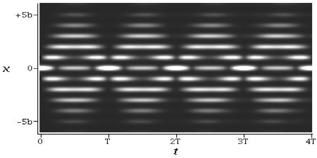
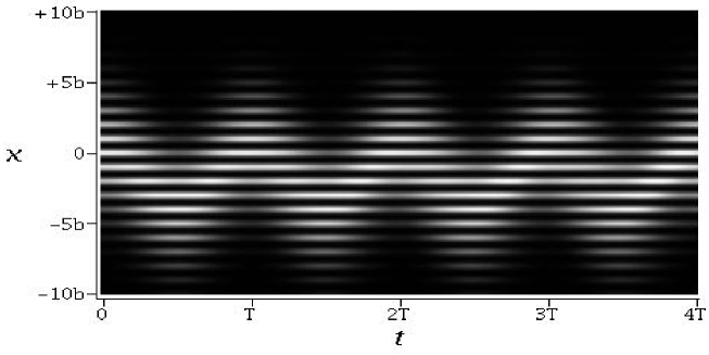
Figure 4. In the top panel we plot the absolute value of the wavefunction $\psi(x,t)$ initially prepared on a single Wannier state for $\eta=0.2$, it turns out that it symmetrically spreads in space and periodically returns to its initial shape without motion of the center of mass.  In the bottom panel we plot the absolute value of the wavefunction initially prepared on several lattice sites for $\eta=0.2$; it turns out that the center of mass oscillates with no marked changes of the shape of the wavefunction.  Here $T$ denotes the Bloch period and $b$ is the distance between two adjacent wells.  Dark regions mean that $|\psi(x,t)|$ is practically zero there, white regions mean that $|\psi(x,t)|$ has its maximum value there.

3.2.2. $\psi_{0}$ is a symmetric wavefunction initially prepared on different lattice cells

We consider a numerical experiment where $N=40$ and $\psi_{0}(x)=\sum_{\ell=0}^{40}c_{\ell}u_{\ell}(x)$, where $c_{\ell}$ have a symmetric Gaussian-type distribution around $\ell=N/2$.  That is the initial value of the coefficients $c_{\ell}(t)$ are given in Table 1, the initial wavefunction $\psi_{0}$ is plotted in Fig. 5, left hand side panel.  In such a case the center of mass $\langle x\rangle^{t}$ oscillates in space and the wavefunction moves with no marked changes in shape (see Fig. 4, bottom panel).  In particular, the function $\langle x\rangle^{t}$ exhibits, for $\eta\not=0$, an oscillating motion where the wavefunction amplitude is modulated (see Fig. 6) and where the oscillating (pseudo-)period (that is the time interval between two consecutive minima or maxima points) depends on $\eta$.  In Fig. 7 we plot the mean value of the oscillating period of the motion of the center of mass after 14 oscillations for $\eta$ in the range $[-0.1,+0.2]$; it turns out that the relative uncertainty with respect to the Bloch period is of order $2.4\cdot 10^{-5}$.

$c_{0}=0$	$c_{10}=0.396\cdot 10^{-3}$	$c_{21}=0.429$	$c_{31}=0.898\cdot 10^{-4}$
$c_{1}=0$	$c_{11}=0.151\cdot 10^{-2}$	$c_{22}=0.347$	$c_{32}=0.177\cdot 10^{-4}$
$c_{2}=0$	$c_{12}=0.502\cdot 10^{-2}$	$c_{23}=0.244$	$c_{33}=0.303\cdot 10^{-5}$
$c_{3}=0$	$c_{13}=0.149\cdot 10^{-1}$	$c_{24}=0.149$	$c_{34}=0$
$c_{4}=0$	$c_{14}=0.363\cdot 10^{-1}$	$c_{25}=0.788\cdot 10^{-1}$	$c_{35}=0$
$c_{5}=0$	$c_{15}=0.788\cdot 10^{-1}$	$c_{26}=0.363\cdot 10^{-1}$	$c_{36}=0$
$c_{6}=0$	$c_{16}=0.149$	$c_{27}=0.149\cdot 10^{-1}$	$c_{37}=0$
$c_{7}=0.303\cdot 10^{-5}$	$c_{17}=0.244$	$c_{28}=0.502\cdot 10^{-2}$	$c_{38}=0$
$c_{8}=0.177\cdot 10^{-4}$	$c_{18}=0.347$	$c_{29}=0.151\cdot 10^{-2}$	$c_{39}=0$
$c_{9}=0.898\cdot 10^{-4}$	$c_{19}=0.429$	$c_{30}=0.396\cdot 10^{-3}$	$c_{40}=0$
	$c_{20}=0.460$

Table 1. Initial values of the coefficients $c_{\ell}:=c_{\ell}(0)$ of the wavefunction.  The initial wavefunction $\psi_{0}$ has a symmetric shape and its width is of order of several lattice periods.

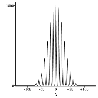
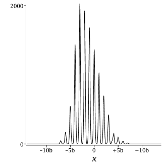
Figure 5. Here we plot the absolute value of the initial wavefunction $\psi_{0}$ prepared on several lattice sites; the left hand side panel corresponds to the symmetric initial wavefunction, the right hand side panel corresponds to the asymmetrical one.

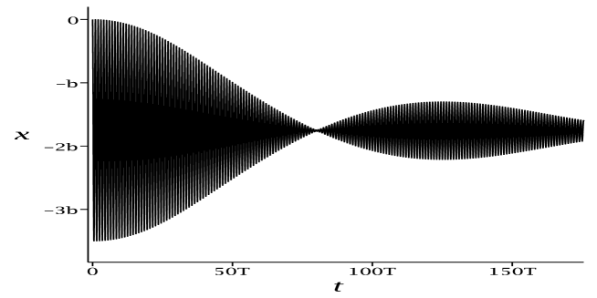
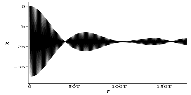
Figure 6. Here we plot the motion of the center of mass of the wavefunction initially prepared on several lattice sites.  The initial wavefunction is a symmetric function.  Top panel corresponds to the case of $\eta=0.1$, bottom panel corresponds to the case of $\eta=0.2$.  The center of mass rapidly oscillates with modulation of the amplitude.  The width of the escillations is in a range lesser or equal to $3b$ is agreement with (24).

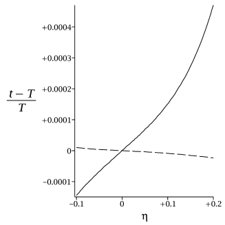
Figure 7. Here we plot the mean value of the pseudo-period of the oscillating motion of the center of mass after 14 oscillations, as function of the effective nonlinearity parameter $\eta$.  Broken line corresponds to the case of a symmetric wavefunction prepared on several lattice sites; it turns out that in such a case the oscillating period is almost constant.  Full line corresponds to the case of an asymmetrical wavefunction prepared on several lattice sites; it turns out that it actually depends on $\eta$.  Here $T$ denotes the Bloch period, while $t$ denotes the oscillating period.

3.2.3. $\psi_{0}$ is an asymmetrical wavefunction initially prepared on different lattice cells

We consider a numerical experiment where $N=40$ and $\psi_{0}(x)=\sum_{\ell=0}^{40}c_{\ell}u_{\ell}(x)$, where $c_{\ell}$ have an asymmetrical Gaussian-type distribution.  That is the initial value of the coefficients $c_{\ell}(t)$ are given in Table 2, the initial wavefunction is plotted in Fig. 5, right hand side panel.  As in the symmetric case the center of mass $\langle x\rangle^{t}$ oscillates in space and the wavefunction moves with no marked changes in shape.  Even in such a case the function $\langle x\rangle^{t}$ exhibits, for $\eta\not=0$, an oscillating motion where the wavefunction amplitude is modulated.  In contrast with the symmetric case the oscillating (pseudo-)period (that is the time interval between two consecutive minima or maxima points) actually depends on $\eta$; in Fig. 7 we plot the mean value of the oscillating period of the center of mass after 14 oscillations for $\eta$ in the range $[-0.1,+0.2]$ and it is not almost constant like in the previous case, in particular it turns out that the relative uncertainty with respect to the Bloch period is of order $4.6\cdot 10^{-4}$, which is 20 times the relative uncertainty observed in the symmetrical case.

$c_{0}=0$	$c_{10}=0.180\cdot 10^{-3}$	$c_{21}=0.252$	$c_{31}=0.175\cdot 10^{-4}$
$c_{1}=0$	$c_{11}=0.814\cdot 10^{-3}$	$c_{22}=0.170$	$c_{32}=0.323\cdot 10^{-5}$
$c_{2}=0$	$c_{12}=0.330\cdot 10^{-2}$	$c_{23}=0.103$	$c_{33}=0$
$c_{3}=0$	$c_{13}=0.121\cdot 10^{-1}$	$c_{24}=0.546\cdot 10^{-1}$	$c_{34}=0$
$c_{4}=0$	$c_{14}=0.414\cdot 10^{-1}$	$c_{25}=0.257\cdot 10^{-1}$	$c_{35}=0$
$c_{5}=0$	$c_{15}=0.133$	$c_{26}=0.106\cdot 10^{-1}$	$c_{36}=0$
$c_{6}=0$	$c_{16}=0.351$	$c_{27}=0.386\cdot 10^{-2}$	$c_{37}=0$
$c_{7}=0$	$c_{17}=0.496$	$c_{28}=0.123\cdot 10^{-2}$	$c_{38}=0$
$c_{8}=0.614\cdot 10^{-5}$	$c_{18}=0.471$	$c_{29}=0.340\cdot 10^{-3}$	$c_{39}=0$
$c_{9}=0.354\cdot 10^{-4}$	$c_{19}=0.411$	$c_{30}=0.826\cdot 10^{-4}$	$c_{40}=0$
	$c_{20}=0.336$

Table 2. Initial values of the coefficients $c_{\ell}:=c_{\ell}(0)$ of the wavefunction.  The initial wavefunction $\psi_{0}$ has an asymmetrical shape and its width is of order of several lattice periods.

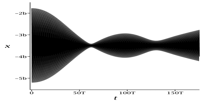
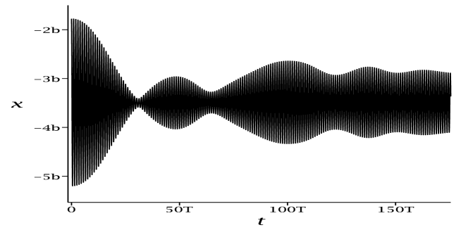
Figure 8. Here we plot the motion of the center of mass of the wavefunction initially prepared on several lattice sites.  The initial wavefunction is a symmetric function.  Top panel corresponds to the case of $\eta=0.1$, bottom panel corresponds to the case of $\eta=0.2$.  The center of mass rapidly oscillates with modulation of the amplitude.  The width of oscillation is in a range lesser or equal to $3b$ is agreement with (24).

4. Conclusion

In this paper we have proved that in the semiclassical limit the $N$-mode approximation (21), corresponding to a discrete nonlinear Schrödinger equation with a finite number of modes, gives the solution of the Gross-Pitaevskii equation (6) for a BEC in a multiple-well lattice in a Stark-type external field.  Furthermore, we have numerically solved the $N$-mode approximation considering a real model, where for some values of the physical parameters the validity of the $N$-mode approximation (21) seems to be justified.  In particular, we have seen that a state initially prepared on several wells have an oscillating behavior with modulated amplitude, the oscillating (pseudo-)period is computed for different values of the nonlinear strength and it turns out that such a period is practically constant when the initial state is a symmetric one; on the other side, such a period actually depends on the nonlinear strength when the initial state is an asymmetrical one.  This observation opens a question about the validity of the method proposed by Cladé et al [9] for the deterimantion of the gravitational constant $g$ by means of the measurement of the oscillating period [12, 20], where it has been assumed that the oscillating period coincides with the Bloch period $T$ independently from the shape of the initial wavefunction and of the value of the nonlinearity strength parameter.

Appendix A Band Functions and Wannier functions

For a generic one-dimensional Bloch operator $H_{B}$ the spectrum is given by a sequence of infinitely many closed intervals named bands.  These intervals are the image of functions named band functions.  The band functions of $H_{B}$ are denoted by ${E}_{n}(k)$, where the quasimomentum $k$ runs in the Brillouin zone $\left[-\frac{\pi}{b},+\frac{\pi}{b}\right]$.  The spectrum of the Bloch operator $H_{B}$ is given by the bands $\sigma(H_{B})=\cup_{n=1}^{\infty}[{E}_{n}^{b},{E}_{n}^{t}]$ where

$${E}_{n}^{b}=\left\{\begin{array}[]{ll}{E}_{n}(0)&\ \mbox{ if }n\mbox{ is even}\\ {E}_{n}(\pi/b)&\ \mbox{ if }n\mbox{ is odd}\end{array}\right.\ ,\ {E}_{n}^{t}=\left\{\begin{array}[]{ll}{E}_{n}(\pi/b)&\ \mbox{ if }n\mbox{ is even}\\ {E}_{n}(0)&\ \mbox{ if }n\mbox{ is odd}\end{array}\right.\,.$$

In the case of potential (2) the band functions may be explicitly computed.  In particular let us look for the Bloch functions of the equation

$$H_{B}\psi={E}\psi\,,\ \ H_{B}=-\frac{\hbar^{2}}{2m}\frac{d^{2}}{dx^{2}}+V_{0}\sin^{2}(k_{L}x)\,.$$

If we set

$${\mathcal{E}}=\left({E}-\frac{1}{2}V_{0}\right)\frac{2m}{\hbar^{2}}\,,\ q=2k_{L}\,,{\tilde{V}}_{0}=\frac{V_{0}m}{\hbar^{2}}=\frac{m\Lambda_{0}E_{r}}{\hbar^{2}}=\frac{1}{2}\Lambda_{0}k_{L}^{2}$$

and recalling that $\sin^{2}(\theta)=\frac{1}{2}\left[1-\cos(2\theta)\right]$ then the Mathieu equation takes the form

$$\left[\tilde{H}_{B}-{\mathcal{E}}\right]\psi=0\ \mbox{ where }\ \tilde{H}_{B}=-\frac{d^{2}}{dx^{2}}-{\tilde{V}}_{0}\cos(qx)\,.$$ (26)

It has a fundamental set of solutions [1]

$$\psi_{1}(x,{\mathcal{E}})=C\left[\frac{4{\mathcal{E}}}{q^{2}},-\frac{{\tilde{V}}_{0}}{q^{2}},\frac{1}{2}qx\right]\ \mbox{ and }\ \psi_{2}(x,{\mathcal{E}})=\frac{2}{q}S\left[\frac{4{\mathcal{E}}}{q^{2}},-\frac{{\tilde{V}}_{0}}{q^{2}},\frac{1}{2}qx\right]$$

where $S$ and $C$ denotes the two Mathieu’s functions, satisfying the conditions

$$\psi_{1}(0,{\mathcal{E}})=1\,,\frac{\partial\psi_{1}(0,{\mathcal{E}})}{\partial y}=0\ \mbox{ and }\ \psi_{2}(0,{\mathcal{E}})=0\,,\frac{\partial\psi_{2}(0,{\mathcal{E}})}{\partial y}=1\,.$$

Hence, the band functions ${\mathcal{E}}_{n}(k)$ associated to the spectral problem (26) are the solutions of the equation $\mu({\mathcal{E}})=\cos(kb)$ where

$$\mu({\mathcal{E}})=\psi_{1}(b,{\mathcal{E}})=C\left[\frac{4{\mathcal{E}}}{q^{2}},-\frac{{\tilde{V}}_{0}}{q^{2}},\pi\right]\,.$$

Let $\lambda=e^{ikb}$, then the equation $\mu({\mathcal{E}})=\cos(kb)$ can be written as $\mu({\mathcal{E}})=\frac{1}{2}(\lambda+\lambda^{-1})$.  We observe that for $k\in\left[0,\frac{\pi}{b}\right]$ then $\sin(kb)=\sqrt{1-\mu^{2}({\mathcal{E}})}$.  The Bloch function is given by [15]

$$\psi(x,{\mathcal{E}})=\frac{\chi(x,{\mathcal{E}})}{\sqrt{N({\mathcal{E}})}}$$

where

$$\chi(x,{\mathcal{E}}) = \psi_{2}(b,{\mathcal{E}})\psi_{1}(x,{\mathcal{E}})+\frac{1}{2}[\lambda({\mathcal{E}})-\lambda^{-1}({\mathcal{E}})]\psi_{2}(x,{\mathcal{E}})$$

$$= \psi_{2}(b,{\mathcal{E}})\psi_{1}(x,{\mathcal{E}})+i\sqrt{1-\mu({\mathcal{E}})^{2}}\psi_{2}(x,{\mathcal{E}})$$

and

$$N({\mathcal{E}})=-\frac{4\pi}{b}\psi_{2}(b,{\mathcal{E}})\frac{d\mu}{d{\mathcal{E}}}\,.$$

We recall that the Bloch function $\psi_{n}(x,k)=\psi(x,{\mathcal{E}}_{n}(k))$, where ${\mathcal{E}}_{n}$ is the band function associated to $\tilde{H}_{B}$, is normalized to one:

$$\frac{2\pi}{b}\int_{0}^{b}|\psi_{n}(x,k)|^{2}dx=1$$

and furthermore it is such that

$$\psi_{n}(x,-k)=\overline{\psi_{n}(x,k)}\,.$$

Finally, the Wannier function on the zero-th cell associated to the $n$-th band is given by

$$w_{n}(x) = \left(\frac{b}{2\pi}\right)^{1/2}\int_{-\pi/b}^{+\pi/b}\psi_{n}(x,k)dk=2\left(\frac{b}{2\pi}\right)^{1/2}\int_{0}^{+\pi/b}\Re\psi_{n}(x,k)dk$$

$$= 2\left(\frac{b}{2\pi}\right)^{1/2}\int_{0}^{\pi/b}\frac{\psi_{2}(b,{\mathcal{E}}_{n}(k))\psi_{1}(x,{\mathcal{E}}_{n}(k))}{\sqrt{N({\mathcal{E}}_{n}(k))}}dk$$

$$= \frac{b}{\sqrt{2}\pi}\int_{0}^{\pi/b}\frac{\sqrt{\psi_{2}(b,{\mathcal{E}}_{n}(k))}\psi_{1}(x,{\mathcal{E}}_{n}(k))}{\sqrt{-\frac{d\mu({\mathcal{E}}_{n}(k))}{d{\mathcal{E}}}}}dk$$

$$= \frac{1}{\sqrt{2}\pi}\int_{{\mathcal{E}}_{n}(0)}^{{\mathcal{E}}_{n}(\pi/b)}\frac{\sqrt{\psi_{2}(b,{\mathcal{E}})}\psi_{1}(x,{\mathcal{E}})\sqrt{-\frac{d\mu({\mathcal{E}})}{d{\mathcal{E}}}}}{\sqrt{1-\mu^{2}({\mathcal{E}})}}d{\mathcal{E}}$$

since the Mathieu functions are real valued when their arguments are real numbers.  In particular,

$$u_{0}^{W}(x):=w_{1}(x)=\frac{1}{\sqrt{2}\pi}\int_{{\mathcal{E}}_{1}^{b}}^{{\mathcal{E}}_{1}^{t}}\frac{\sqrt{\psi_{2}(b,{\mathcal{E}})}\psi_{1}(x,{\mathcal{E}})\sqrt{-\frac{d\mu({\mathcal{E}})}{d{\mathcal{E}}}}}{\sqrt{1-\mu^{2}({\mathcal{E}})}}d{\mathcal{E}}\,.$$

Acknowledgements. This work is partially supported by Gruppo Nazione per la Fisica Matematica (GNFM-INdAM).  The author is grateful for the hospitality of the Isaac Newton Institute for Mathematical Sciences where part of this paper was written.

References

- [1] M. Abramowitz, and I.A. Stegun, Handbook of Mathematical Functions: with Formulas, Graphs, and Mathematical Tables, (Dover Books on Mathematics: 1965).
- [2] G.L. Alfimov, P.G. Kevrekidis, V.V. Konotop, and M. Salerno, Wannier functions analysis of the nonlinear Schrödinger equation with a periodic potential, Phys. Rev. E 66, 046608 (2002).
- [3] , D.J. Boers, B. Goedeke, D. Hinrichs, and M. Holthaus, Mobility edges in bichromatic optical lattices, Phys. Rev. A 75, 063404 (2007).
- [4] I. Bloch, Ultracold quantum gases in optical lattices, Nature Phys. 1 23-30 (2005).
- [5] I. Bloch, Quantum choerence and entanglement with ultracold atoms in optical lattices, Nature 453 1016-1022 (2008).
- [6] T.Cazenave, and F.B. Weissler, The Cauchy problem for the nonlinear Schrödinger equation in , Manuscripta Math. 61, 477-494 (1988).
- [7] T. Cazenave, Semilinear Schrodinger Equations (Courant Lecture Notes: 2003).
- [8] J. Callaway, Quantum theory of the solis state. Part B. (Academi Press: New York) (1974).
- [9] C. Cladé, S. Guellati-Khélifa, C. Schwob1, F. Nez, L. Julien, and F. Biraben, A promising method for the measurement of the local acceleration of gravity using Bloch oscillations of ultracold atoms in a vertical standing wave, Europhys. Lett. 71 730 (2005).
- [10] C. Cladé, Bloch oscillations in atom interferometry, Proceedings of the International School of Physics ”Enrico Fermi” edited by G.M. Tino and M.A. Kasevich, 188, 419-455 (2014).
- [11] A. Eckardt, M. Holthaus, H. Lignier, A. Zenesini, D. Ciampini, O. Morsch, and E. Arimondo, Exploring dynamic localization with a Bose-Einstein condensate, Phys. Rev. A 79, 013611 (2009).
- [12] G. Ferrari, N. Poli, F. Sorrentino, and G.M. Tino, Long-lived Bloch oscillations with bosonic atoms and application to gravity meausrement at the micrometer scale, Phys. Rev. Lett. 97 060402 (2006).
- [13] J.B. Fixler, G.T. Foster, J.M. McGuirk, and M.A. Kasevich, Atom Interferometer Measurement of the Newtonian Constant of Gravity, Science 315 74-77 (2007).
- [14] R. Fukuizumi, and A. Sacchetti, Stationary States for Nonlinear Schrödinger Equations with Periodic Potentials, J. Stat. Phys. 156 707-738 (2014).
- [15] W. Kohn, it Analytic properties of Bloch waves and Wannier functions, Phys. Rev. 115 809-821 (1959).
- [16] G. Lamporesi, A. Bertoldi, L. Cacciapuoti, M. Prevedelli, and G.M. Tino, Determination of the Newtonian Gravitational Constant Using Atom Interferometry, Phys. Rev. Lett. 100 050801 (2008).
- [17] J.M. McGuirk, G.T. Foster, J.B. Fixler, M.J. Snadden, and M.A. Kasevich, Sensitive absolute-gravity gradiometry using atom interferometry, Phys. Rev. A 65 033608 (2002).
- [18] D. Pelinovsky, G. Schneider, and R.S. MacKay, Justification of the lattice equation for a nonlinear elliptic problem with a periodic potential, Commun. Math. Phys. 284 803-831 (2008).
- [19] D. Pelinovsky, G. Schneider, Bounds on the tight-binding approximation for the Gross-Pitaevskii equation with a periodic potential, J. of Diff. Eq. 248 837-849 (2010).
- [20] N. Poli, F.Y. Wang, M.G. Tarallo, A. Alberti, M. Prevedelli, and G.M. Tino, Precision measurement of gravity with cold atoms in an optical lattice and comparison with a classical gravimeter, Phys. Rev. Lett. 106 038501 (2011).
- [21] M. Raizen, C. Salomon, and Q. Niu, New light on quantum transport, Phys. Today 50 30-34 (1997).
- [22] G. Rosi, F. Sorrentino, L. Cacciapuoti, M. Prevedelli, and G.M Tino, Precision measurement of the Newtonian gravitational constant using cold atoms, Nature 510 518-521 (2014).
- [23] M. Saba, T.A. Pasquini, C. Sanner, Y. Shin, W. Ketterle, and D.E. Pritcard, Light scattering to determine the relative phase of two Bose-Einstein condensates, Science 307 1945-1948 (2005).
- [24] A. Sacchetti, Nonlinear doublewell Schrödinger equations in the semiclassical limit, J. Stat. Phys. 119 1347-1382 (2005).
- [25] A. Sacchetti, Nonlinear Schrödinger equations with multiple-well potential, Physica D 241 1815-1824 (2012).
- [26] L. Salasnich, A. Parola, and L. Reatto, Effective wave equations for the dynamics of cigar-shaped and disk-shaped Bose condensates Phys. Rev. A 65, 043614 (2002).
- [27] Y. Shin, M. Saba, T.A. Pasquini, W. Ketterle, D.E. Pritchard, and A.E. Leanhardt, Atom Interferometry with Bose-Einstein Condensates in a Double-Well Potential, Phys. Rev. Lett. 92 050405 (2004).
- [28] F. Sorrentino, A. Alberti, G. Ferrari, V.V. Ivanov, N. Poli, M. Schioppo, and G.M. Tino, Quantum sensor for atom-surface interactions below , Phys. Rev. A 79 013409 (2009).
- [29] G.M. Tino, Testing gravity with atom interferometry, Proceedings of the International School of Physics ”Enrico Fermi” edited by G.M. Tino and M.A. Kasevich, 188 457-491 (2014).
- [30] M.I. Weinstein, and J.B. Keller, Asymptotic Behavior of stability regions for Hill’s equation, SIAM J. Appl. Math. 47 941-958 (1987)