WUF-HEP-15-13 EPHOU-15-011 Gauge coupling unification in $SO(32)$ heterotic string theory with magnetic fluxes

1 Introduction

Gauge coupling unification is a familiar tool to search for the underling theory of the standard model such as the Grand unified theory (GUT) or string theory. For example, in the light of the observed values of gauge couplings, the three gauge couplings are unified with the GUT normalization of $U(1)_{Y}$ at the so-called GUT scale, $2\times 10^{16}$ GeV in the low-energy or multi-TeV scale minimal supersymmetric standard model (MSSM). On the other hand, the three gauge couplings are not unified with the GUT normalization of $U(1)_{Y}$ in the standard model (SM).

Superstring theory also has a certain prediction. In particular, in 4D low-energy effective field theory derived from heterotic string theory, the gauge couplings at tree level are unified up to Kač-Moody levels $\kappa_{a}$ at the string scale [1], which is of ${\cal O}(10^{17})$ GeV [2]. This prediction is very strong. In order to explain the experimental values, we may need some corrections, e.g. stringy threshold corrections [3, 4, 5]. (See for numerical studies e.g. Refs. [6, 7].) Then, we may need ${\cal O}(10)$ of moduli values. When some moduli values are of ${\cal O}(10)$ or larger, the string coupling may become strong and peturbative description may not be valid.

On the other hand, in D-brane models, gauge couplings seem to be independent of each other for gauge sectors, which originate from different sets of D-branes. Thus, one may be able to fit parameters such as moduli values in order to explain the experimental values of three gauge couplings, although there may appear some relations and/or constraints [9, 10] in a certain type of models.

Here, we study another possible correction within the framework of heterotic string theory. Recently, we carried out systematic analysis towards realistic models within the framework of $SO(32)$ heterotic string theory on the toroidal compactification with magnetic fluxes [11]. In such a type of model building, we have constructed the models which have the gauge symmetry including $SU(3)\times SU(2)\times U(1)_{Y}$ and three generations of quarks and leptons as chiral massless spectra. Furthermore, in this paper we show that the gauge couplings depend on magnetic fluxes in this type of $SO(32)$ heterotic string theory. That is, gauge couplings can be non-universal at the string scale and non-universal parts depend on the Kähler moduli, although $E_{8}\times E_{8}$ heterotic string theory with magnetic fluxes can not lead to non-universal gauge couplings between $SU(3)$ and $SU(2)$ appearing in one $E_{8}$. Such non-universal corrections can make the gauge coupling prediction consistent with experimental values. Although such possibilities are proposed in Ref. [13], we study numerically the gauge couplings of $SU(3)\times SU(2)\times U(1)_{Y}$ in more realistic models.

This paper is organized as follows. In section 2, we review 4D low-energy effective field theory derived from $SO(32)$ heterotic string theory with magnetic fluxes. We also review on our model building towards realistic models, which have the gauge symmetry including $SU(3)\times SU(2)\times U(1)_{Y}$ and three chiral generations of quarks and leptons as well as vector-like matter fields in massless spectra. In section 3, we study the gauge couplings and show how non-universal gauge couplings appear in our models. In section 4, we study numerically the gauge couplings in explicit models. Section 5 is devoted to conclusions and discussions.

2 $SO(32)$ heterotic string theory on tori with $U(1)$ magnetic fluxes

In this section, we give a review on the low-energy effective field theory derived from $SO(32)$ heterotic string theory on factorizable tori with $U(1)$ magnetic fluxes. We also show the consistency conditions for $U(1)$ magnetic fluxes which give the constraints for the heterotic string models. (See for details of model construction e.g., Ref. [11].)

2.1 Low-energy effective action of $SO(32)$ heterotic string theory

First of all, we show the bosonic part of $10$D effective supergravity action derived from the $SO(32)$ heterotic string theory on a general complex manifold $M$ with multiple $U(1)$ magnetic fluxes. By calculating the relevant scattering amplitudes on the worldsheet up to of order ${\cal O}(\alpha^{\prime})$, we obtain the string-frame bosonic action in the notation of Refs. [13, 14, 15],

$$S_{\rm bos} =\frac{1}{2\kappa_{10}^{2}}\int_{M^{(10)}}e^{-2\phi_{10}}\left[R+4d\phi_{10}\wedge\ast d\phi_{10}-\frac{1}{2}H\wedge\ast H\right]$$

$$-\frac{1}{2g_{10}^{2}}\int_{M^{(10)}}e^{-2\phi_{10}}{\rm tr}(F\wedge\ast F),$$ (1)

where the gauge and gravitational couplings are set by $g_{10}^{2}=2(2\pi)^{7}(\alpha^{{}^{\prime}})^{3}$ and $2\kappa_{10}^{2}=(2\pi)^{7}(\alpha^{{}^{\prime}})^{4}$, respectively. The string coupling is determined by the vacuum expectation value of the ten-dimensional dilaton $\phi_{10}$, that is, $g_{s}=e^{\langle\phi_{10}\rangle}$. The field-strength of $SO(32)$ gauge group $F$ has the index of vector-representation, which can be normalized as ${\rm tr}_{v}(T^{a}T^{b})=2\delta^{ab}$. In addition, the heterotic three-form field strength $H$ is defined by

$$H =dB^{(2)}-\frac{\alpha^{{}^{\prime}}}{4}(w_{\rm YM}-w_{L}),$$ (2)

where the part of $\alpha^{\prime}$ corrections are characterized by the gauge and gravitational Chern-Simons three-forms, $w_{\rm YM}$ and $w_{L}$, respectively.

By the ten-dimensional Hodge duality, the Kalb-Ramond two-form $B^{(2)}$ and its dual six-form $B^{(6)}$ are related as,

$$\ast dB^{(2)}=e^{2\phi_{10}}dB^{(6)}.$$ (3)

Then, from the $10$D bosonic action (1), we can extract the kinetic term of Kalb-Ramond field,

$$S_{\rm kin}+S_{\rm WZ} =-\frac{1}{4\kappa_{10}^{2}}\int_{M^{(10)}}e^{2\phi_{10}}dB^{(6)}\wedge\ast dB^{(6)}$$

$$+\frac{\alpha~{}{{}^{\prime}}}{8\kappa_{10}^{2}}\int_{M^{(10)}}B^{(6)}\wedge\left({\rm tr}F^{2}-{\rm tr}R^{2}-4(2\pi)^{2}\sum_{a}N_{a}\delta(\Gamma_{a})\right),$$ (4)

where we have added the Wess-Zumino terms induced by the magnetic sources for the Kalb-Ramond field $B^{(6)}$, i.e., stacks of $N_{a}$ five-branes with their tension being $T_{5}=((2\pi)^{5}(\alpha^{{}^{\prime}})^{3})^{-1}$. Note that these heterotic five-branes wrap the holomorphic two-cycles $\Gamma_{a}$ and their Poincáre dual four-forms are denoted by $\delta(\Gamma_{a})$.

When we study $SO(32)$ heterotic string theory on three 2-tori, $M=(T^{2})_{1}\times(T^{2})_{2}\times(T^{2})_{3}$, the tadpole cancellation is obtained by solving the equation of motion for the Kalb-Ramond field,

$$\int_{(T^{2})_{i}\times(T^{2})_{j}}\left({\rm tr}\bar{F}^{2}-4(2\pi)^{2}\sum_{a}N_{a}\delta(\Gamma_{a})\right)=0,$$ (5)

where $\bar{F}$ represents for the internal $U(1)$ gauge field strengths. These conditions should be satisfied on any four-cycles $(T^{2})_{i}\times(T^{2})_{j}$ with $i\neq j$, $i,j=1,2,3$. However, if the nonvanishing fluxes are not canceled by themselves, five-branes would contribute to the tadpole cancellation [16].

2.2 Axionic coupling through the Green-Schwarz term

In addition to the effective action (1), the loop effects induce the Green-Schwarz term at the string frame [17, 18],

$$S_{\rm GS}=\frac{1}{24(2\pi)^{5}\alpha^{\prime}}\int B^{(2)}\wedge X_{8},$$ (6)

whose normalization factor is determined by its S-dual type I theory as shown in [19] and the anomaly eight-form $X_{8}$ reads,

$$X_{8}=\frac{1}{24}{\rm Tr}F^{4}-\frac{1}{7200}({\rm Tr}F^{2})^{2}-\frac{1}{240}({\rm Tr}F^{2})({\rm tr}R^{2})+\frac{1}{8}{\rm tr}R^{4}+\frac{1}{32}({\rm tr}R^{2})^{2},$$ (7)

where “Tr” stands for the trace in the adjoint representations of the $SO(32)$ gauge group.

As pointed out in Refs. [20, 13], the gauge and gravitational anomalies for the (non-)Abelian gauge groups are canceled by the above Green-Schwarz term (6) and the tadpole condition (5). It is remarkable that even if the Abelian gauge symmetries are anomaly-free, the Abelian gauge bosons may become massive due to the Green-Schwarz coupling given by Eq. (6). Therefore, in order to ensure that the hypercharge gauge boson is massless, they should not couple to the axions which are hodge dual to the Kalb-Ramond fields.

Let us study the couplings between the hypercharge $U(1)_{Y}$ gauge boson and the axions, explicitly. First of all, we decompose the $SO(32)$ gauge group into the standard-like model gauge group,

$$SO(32)\rightarrow SU(3)_{C}\otimes SU(2)_{L}\otimes_{a=1}^{13}U(1)_{a},$$ (8)

which can be realized by inserting all the multiple $U(1)$ constant magnetic fluxes.

Within the $16$ Cartan elements, $H_{i}$ ($i=1,\cdots,16$) in $SO(32)$ gauge group, the Cartan elements of $SU(3)$ are chosen along $H_{1}-H_{2}$, $H_{1}+H_{2}-2H_{3}$ and that of $SU(2)$ is taken as $H_{5}-H_{6}$, whereas the other Cartan directions of $SO(32)$ are defined as,

$$U(1)_{1}:\,\,\frac{1}{\sqrt{2}}(0,0,0,0,1,1;0,0,\cdots,0),$$

$$U(1)_{2}:\,\,\frac{1}{2}(1,1,1,1,0,0;0,0,\cdots,0),$$

$$U(1)_{3}:\,\,\frac{1}{\sqrt{12}}((1,1,1,-3,0,0;0,0,\cdots,0),$$

$$U(1)_{4}:\,\,(0,0,0,0,0,0;1,0,\cdots,0),$$

$$U(1)_{5}:\,\,(0,0,0,0,0,0;0,1,\cdots,0),$$

$$\qquad\vdots$$

$$U(1)_{13}:\,\,(0,0,0,0,0,0;0,0,\cdots,1),$$ (9)

in the basis $H_{i}$.

Furthermore, when these $U(1)$ fluxes are inserted along the Cartan direction of $SO(32)$, the field strengths of $U(1)$’s are also decomposed into the four-and extra-dimensional parts $f$, $\bar{f}$, respectively. Then we can dimensionally reduce the one-loop Green-Schwarz term (6) to

$$S_{\rm GS}=\, \frac{1}{(2\pi)^{3}l_{s}^{2}}\int_{M^{(10)}}B^{(2)}\wedge\frac{1}{144}({\rm Tr}F\bar{f}^{3})$$ (10)

$$-\frac{1}{(2\pi)^{3}l_{s}^{2}}\int_{M^{(10)}}B^{(2)}\wedge\frac{1}{2880}({\rm Tr}F\bar{f})\wedge\left(\frac{1}{15}{\rm Tr}\bar{f}^{2}+{\rm tr}{\bar{R}}^{2}\right)$$ (11)

$$+\frac{1}{(2\pi)^{3}l_{s}^{2}}\int_{M^{(10)}}B^{(2)}\wedge\Bigl{[}\frac{1}{96}({\rm Tr}F^{2}\bar{f}^{2})-\frac{1}{43200}({\rm Tr}F\bar{f})^{2}\Bigl{]}$$ (12)

$$-\frac{1}{(2\pi)^{3}l_{s}^{2}}\int_{M^{(10)}}B^{(2)}\wedge\frac{1}{5760}({\rm Tr}F^{2})\wedge\left(\frac{1}{15}{\rm Tr}\bar{f}^{2}+{\rm tr}{\bar{R}}^{2}\right)$$ (13)

$$+\frac{1}{(2\pi)^{3}l_{s}^{2}}\int_{M^{(10)}}B^{(2)}\wedge\frac{1}{384}({\rm tr}R^{2})\wedge\left({\rm tr}\bar{R}^{2}-\frac{1}{15}{\rm Tr}{\bar{f}}^{2}\right),$$ (14)

where $l_{s}=2\pi\sqrt{\alpha^{\prime}}$ and $F$ denote the field strengths of $SU(3)_{C}$, $SU(2)_{L}$ and $U(1)_{a}$, $(a=1,\cdots,13)$.

From here, we write the Kalb-Ramond field $B^{(2)}$ and internal $U(1)_{a}$ field strengths $\bar{f}_{a}$, $(a=1,\cdots,13)$ in the basis of Kähler forms $w_{i}$ on tori $(T^{2})_{i}$

$$B^{(2)}=b_{S}^{(2)}+l_{s}^{2}\sum_{i=1}^{3}b_{i}^{(0)}w_{i},$$

$$\bar{f}_{a}=2\pi d_{a}\sum_{i=1}^{3}m_{a}^{(i)}w_{i},$$ (15)

where $d_{a}$ are normalization factors appeared in the basis $H_{i}$ (9) and $m_{a}^{(i)}$ are the $U(1)_{a}$ fluxes constrained by the Dirac quantization condition. From the Eqs. (10) and (11), we can extract the Stueckelberg couplings between the $U(1)$ gauge fields and the universal axion $b_{S}^{(0)}$ which is the hodge dual of the tensor field $b_{S}^{(2)}$ ,

$$\frac{1}{3(2\pi)^{3}l_{s}^{2}}\int b_{S}^{(2)}\wedge \Bigl{[}{\rm tr}T_{1}^{4}{\bar{f}}_{1}^{3}f_{1}+\left({\rm tr}T_{2}^{4}{\bar{f}}_{2}^{3}+3({\rm tr}T_{2}^{2}T_{3}^{2}){\bar{f}}_{2}{\bar{f}}_{3}^{2}+({\rm tr}T_{2}T_{3}^{3}){\bar{f}}_{3}^{3}\right)f_{2}$$

$$+\left({\rm tr}T_{3}^{4}{\bar{f}}_{3}^{3}+3({\rm tr}T_{2}T_{3}^{3}){\bar{f}}_{2}{\bar{f}}_{3}^{2}+3({\rm tr}T_{2}^{2}T_{3}^{2}){\bar{f}}_{2}^{2}{\bar{f}}_{3}\right)f_{3}+\sum_{c=4}^{13}{\rm tr}T_{c}^{4}{\bar{f}}_{c}^{3}f_{c}\Bigl{]},$$ (16)

which implies that one of the multiple $U(1)$ gauge fields absorbs the universal axion and become massive. As shown in Sec. 3, the hypercharge $U(1)_{Y}$ is identified with the linear combinations of multiple $U(1)$’s, i.e., $U(1)_{Y}=\frac{1}{6}(U(1)_{3}+3\sum_{c}U(1)_{c})$, where the summation over $c$ depends on the concrete models. In such cases, the $U(1)_{Y}$ gauge field becomes massless under

$$6{\rm tr}(T_{3}^{4})m_{3}^{(1)}m_{3}^{(2)}m_{3}^{(3)}+3{\rm tr}(T_{2}T_{3}^{3})d_{ijk}m_{2}^{(i)}m_{3}^{(j)}m_{3}^{(k)}+3{\rm tr}(T_{2}^{2}T_{3}^{2})d_{ijk}m_{2}^{(i)}m_{2}^{(j)}m_{3}^{(k)}$$

$$+18\sum_{c}{\rm tr}(T_{c}^{4})m_{c}^{(1)}m_{c}^{(2)}m_{c}^{(3)}=0,$$ (17)

where $d_{ijk}$ denotes the intersection number and there appear the non-vanishing intersection numbers of 2-tori, $d_{ijk}=1$ ($i\neq j\neq k$).

In addition to the universal axion, other axions also appear from the associated internal two-cycles, which are known as the Kähler axions. When the dual field $B^{(6)}$ is expanded as

$$B^{(6)}=l_{s}^{6}b_{S}^{(0)}{\rm vol}(M)+l_{s}^{4}\sum_{k=1}^{3}b_{k}^{(2)}\hat{w}_{k},$$ (18)

where $\hat{w}_{k}$ are the Hodge dual four-forms of the Kähler forms, we can extract the axionic couplings between Kähler axions and the $U(1)$ gauge bosons through Eq. (4),

$$\frac{1}{l_{s}^{2}}\int b_{i}^{(2)}\wedge\sum_{a=1}^{13}f_{a}m_{a}^{(i)},$$ (19)

which lead to the following $U(1)_{Y}$ massless condition,

$$m_{3}^{(i)}+3\sum_{c=4}^{13}m_{c}^{(i)}=0,$$ (20)

with $i=1,2,3$.

2.3 Model building and constraints

Here we review our approach to construct realistic models. (See the detail for Ref. [11].) So far, we introduce the magnetic fluxes $m^{(i)}_{a}$ along all $U(1)_{a}$ for $a=1,\cdots,13$. In our model, such magnetic fluxes break $SO(32)$ into $SU(3)_{C}\times SU(2)_{L}\times\prod_{a=1}^{13}U(1)_{a}$ and a certain linear combination of $\prod_{a=1}^{13}U(1)_{a}$ corresponds to $U(1)_{Y}$. However, the degenerate magnetic fluxes lead to the enhancement of gauge symmetry e.g., $SU(4)\times SU(2)\times SU(2)$ in the visible sector. In such a case, we introduce Wilson lines to break this remaining large gauge group into $SU(3)_{C}\times SU(2)_{L}\times U(1)_{Y}$.

In addition to gauge symmetry breaking, non-vanishing magnetic fluxes can realize the $4$D chiral theory, where the number of zero modes is determined by their $U(1)$ charges and magnetic fluxes. The relevant matter contents in the SM reside in the adjoint and vector representations of $SO(12)$ in $SO(32)$ and their generation numbers are given by

$$\begin{array}[]{ll}m_{Q_{1}}=\prod_{i=1}^{3}m_{Q_{1}}^{i}=\prod_{i=1}^{3}(m_{1}^{i}+m_{2}^{i}+m_{3}^{i}),&m_{Q_{2}}=\prod_{i=1}^{3}m_{Q_{2}}^{i}=\prod_{i=1}^{3}(-m_{1}^{i}+m_{2}^{i}+m_{3}^{i}),\\ m_{L_{1}}=\prod_{i=1}^{3}m_{L_{1}}^{i}=\prod_{i=1}^{3}(m_{1}^{i}+m_{2}^{i}-3m_{3}^{i}),&m_{L_{2}}=\prod_{i=1}^{3}m_{L_{2}}^{i}=\prod_{i=1}^{3}(-m_{1}^{i}+m_{2}^{i}-3m_{3}^{i}),\\ m_{u_{R_{1}}^{c}}=\prod_{i=1}^{3}m_{u_{R_{1}}^{c}}^{i}=\prod_{i=1}^{3}(-4m_{3}^{i}),&m_{n_{1}}=\prod_{i=1}^{3}m_{n_{1}}^{i}=\prod_{i=1}^{3}(2m_{1}^{i}),\\ m_{d_{R_{1}}^{c}}=\prod_{i=1}^{3}m_{d_{R_{1}}^{c}}^{i}=\prod_{i=1}^{3}(2m_{2}^{i}+2m_{3}^{i}),&m_{d_{R_{2}}^{c}}=\prod_{i=1}^{3}m_{d_{R_{2}}^{c}}^{i}=\prod_{i=1}^{3}(-2m_{2}^{i}+2m_{3}^{i}),\\ m_{L_{3}^{a}}=\prod_{i=1}^{3}m_{L_{3}^{a}}^{i}=\prod_{i=1}^{3}(m_{1}^{i}-m_{a}^{i}),&m_{L_{4}^{a}}=\prod_{i=1}^{3}m_{L_{4}^{a}}^{i}=\prod_{i=1}^{3}(-m_{1}^{i}-m_{a}^{i}),\\ m_{u_{R_{2}}^{c\,a}}=\prod_{i=1}^{3}m_{u_{R_{2}}^{c\,a}}^{i}=\prod_{i=1}^{3}(-m_{2}^{i}-m_{3}^{i}-m_{a}^{i}),&m_{d_{R_{3}}^{c\,a}}=\prod_{i=1}^{3}m_{d_{R_{3}}^{c\,a}}^{i}=\prod_{i=1}^{3}(-m_{2}^{i}-m_{3}^{i}+m_{a}^{i}),\\ m_{e_{R_{1}}^{c\,a}}=\prod_{i=1}^{3}m_{e_{R_{1}}^{c\,a}}^{i}=\prod_{i=1}^{3}(-m_{2}^{i}+3m_{3}^{i}+m_{a}^{i}),&m_{n_{2}^{a}}=\prod_{i=1}^{3}m_{n_{2}^{a}}^{i}=\prod_{i=1}^{3}(-m_{2}^{i}+3m_{3}^{i}-m_{a}^{i}),\end{array}$$ (28)

where $Q_{1,2}$ are the left-handed quarks, $L_{1,2},L_{3,4}^{a}$ are the charged leptons and/or Higgs, $u_{R_{1}}^{c},u_{R_{2}}^{c\,a}$ are the charge conjugate of right-handed up type quarks, $d_{R_{1,2}}^{c},d_{R_{3}}^{c\,a}$ are the charge conjugate of right-handed down type quarks, $e_{R_{1}}^{c\,a}$ are the charge conjugate of right-handed leptons, $n_{1},n_{2}^{a}$ are the singlets in the standard model gauge groups.

It is remarkable that there are constraints for these $U(1)$ magnetic fluxes. First one is that the $U(1)_{Y}$ massless conditions (17) and (20) by taking account of the axionic couplings with $U(1)_{Y}$ gauge boson. Furthermore, there are the tadpole conditions given by Eq. (5). When the heterotic five-branes are absent in our system, the Eq. (5) is rewritten as

$$\sum_{a=1}^{13}m_{a}^{(i)}m_{a}^{(j)}=0,\,\,i\neq j,\,\,\,(i,j=1,2,3),$$ (29)

which are required from the consistencies of heterotic string theory.

Without the existence of the heterotic five-branes, it is known that $U(1)$ magnetic fluxes satisfy the so-called K-theory constraints, e.g., Ref. [13],

$$\sum_{a=1}^{13}m_{a}^{i}=0\quad({\rm mod}~{}2),$$ (30)

for $i=1,2,3$. These K-theory constraints are discussed in the S-dual to the $SO(32)$ heterotic string theory, that is, type I string theory. (See for instance, Ref. [21, 22].)

Finally, non-vanishing magnetic fluxes generically induce the non-vanishing Fayet-Illipoulous (FI) terms for $U(1)_{a}$ with $a=1,2,\cdots,13$. Even if such FI terms are not canceled by themselves, they may be able to be canceled by the vacuum expectation values (VEVs) of scalar fields in the hidden sector.

3 Gauge couplings in heterotic string

In this section, we show the formula of gauge kinetic functions in our model. After dimensionally reducing the $10$D effective action (1) as well as the one-loop GS term (6), it is found that the gauge kinetic functions of $SU(3)_{C}$ and $SU(2)_{L}$ receive the different one-loop threshold corrections depending on the abelian fluxes, while that of $U(1)_{Y}$ do not receive such corrections due to the vanishing axionic couplings with $U(1)_{Y}$ gauge boson.

3.1 Gauge couplings at tree-level

After compactifying on a $6$D internal manifold M with volume ${\rm Vol(M)}$, the $4$D reduced Planck scale $M_{\rm Pl}$ and the gauge coupling constant $g_{4}$ can be extracted as

$$M_{\rm Pl}^{2}=\frac{g_{s}^{-2}{\rm Vol(M)}}{2\kappa_{10}^{2}},$$

$$g_{4}^{-2}=g_{s}^{-2}{\rm Vol(M)}g_{10}^{-2},$$ (31)

which lead to the following relation between the string scale $M_{s}=1/l_{s}$ with $l_{s}=2\pi\sqrt{\alpha^{\prime}}$ being the typical string length, and the Planck-scale,

$$M_{s}^{2}=\frac{M_{\rm Pl}^{2}}{4\pi\alpha_{4}^{-1}},$$ (32)

where $\alpha_{4}^{-1}=4\pi g_{4}^{-2}$. Since the four-dimensional gauge coupling is determined by the VEV of the dilaton at the tree-level, $\langle{\rm Re}S\rangle=g_{4}^{-2}$, where

$$S=\frac{1}{2\pi}\left(\frac{e^{-2\phi_{10}}{\rm Vol(M)}}{l_{s}^{6}}+ib_{S}^{(0)}\right),$$ (33)

with $b_{S}^{(0)}$ being the universal axion, the string scale is roughly estimated as,

$$M_{s}\simeq 1.4\times 10^{17}\,{\rm GeV},$$ (34)

from Eq. (32) by employing $M_{\rm Pl}=2.435\times 10^{18}\,{\rm GeV}$ and the four-dimensional gauge coupling constant, $\alpha_{4}^{-1}\simeq 25$, implied by the renormalization group (RG) equations of the MSSM. As mentioned in the introduction, the gauge couplings of SM gauge groups are different from each other at the string scale as illustrated in Fig. 1 under the assumption that the SUSY is broken at the TeV scale and the $U(1)_{Y}$ gauge coupling is normalized as satisfying the so-called GUT relation. In Fig. 1, we involve two-loop effects to the RG equations. On the other hand, when the SUSY is broken at the string scale, the behavior of gauge couplings from the electroweak scale to the string scale is obeyed by the renormalization group equations of the standard model. As seen in Fig. 2, the gaps between the gauge couplings of non-abelian gauge groups are better than that of MSSM. However, it requires the slight corrections to be coincide with the unified one at the string scale. In this case, the string scale is estimated as $M_{s}\simeq 1.0\times 10^{17}$ GeV by use of $\alpha_{4}^{-1}\simeq 45$. We also employ the experimental values such as the gauge coupling of $SU(3)$, $\alpha_{SU(3)_{C}}^{-1}\simeq 0.1184$, the Weinberg angle ${\rm sin}^{2}\theta\simeq 0.231$ and the fine-structure constant $\alpha\simeq 1/128$ at the electroweak scale [23] in Figs. 1 and 2.

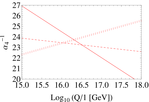
Figure 1: RG flow of the gauge couplings in the MSSM at the two-loop level. These lines show the gauge coupling of $U(1)_{Y}$ (thick line), $SU(2)_{L}$ (dashed line) and $SU(3)_{C}$ (dotted line), respectively. Here, we include the error bar associated with the QCD coupling $\alpha_{SU(3)_{C}}^{-1}$ [23].

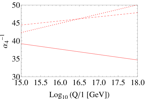
Figure 2: RG flow of the gauge couplings in the SM at the two-loop level. These lines show the gauge coupling of $U(1)_{Y}$ (thick line), $SU(2)_{L}$ (dashed line) and $SU(3)_{C}$ (dotted line), respectively.

3.2 The one-loop threshold corrections

As shown in the previous section, the dilaton $S$ gives the universal gauge kinetic function. However, the Green-Schwarz term $(\ref{eq:GS})$, in particular (12) and (13), can lead to non-universal gauge kinetic functions [13]. Indeed, we obtain the non-universal axionic couplings,

$$S_{\rm GS}\supset \frac{1}{(2\pi)^{3}}\sum_{k=1}^{3}\int_{M^{1,3}}b_{k}^{(0)}{\rm tr}_{SU(3)}F^{2}\int_{T^{2}\times T^{2}\times T^{2}}w_{k}\wedge\left(\frac{1}{8}{\rm tr}(T_{2}^{2})\bar{f}_{2}^{2}\right)$$

$$+\frac{1}{(2\pi)^{3}}\sum_{k=1}^{3}\int_{M^{1,3}}b_{k}^{(0)}{\rm tr}_{SU(2)}F^{2}\int_{T^{2}\times T^{2}\times T^{2}}w_{k}\wedge\left(\frac{1}{4}{\rm tr}(T_{1}^{2})\bar{f}_{1}^{2}\right),$$ (35)

which lead to the non-universal gauge kinetic functions. This is because we insert the different $U(1)$ fluxes between $U(1)_{1}$ and $U(1)_{2}$ Cartan directions. Such structures are typical in $SO(32)$ heterotic string theory which is expected as the S-dual of type I string theory with several D-branes. However, the non-universal gauge kinetic functions for $SU(3)_{C}$ and $SU(2)_{L}$ cannot be seen in $E_{8}\times E_{8}$ heterotic string theory due to the trace identities, ${\rm Tr}(F^{4})=\frac{1}{100}({\rm Tr}(F^{2}))^{2}$, where $F$ denotes the gauge field strength of $E_{8}$. From this trace identities, Eq. (12) is regarded as the type of Eq. (13). Therefore, the gauge kinetic functions of $SU(3)_{C}$ and $SU(2)_{L}$ are equal to each other. It might be preferred in the non-supersymmetric theory such as the standard model from the Fig. 2, although some other threshold corrections are required to unify the gauge couplings.

When we define the Kähler moduli as

$$T_{k}=t_{k}+ib_{k}^{(0)},$$ (36)

where $t_{k}$ corresponds to the volume of $(T^{2})_{k}$, the gauge kinetic functions of the $SU(3)_{C}$ and $SU(2)_{L}$ become

$$f_{SU(3)_{C}}=S+\beta_{3}^{k}T^{k},$$

$$f_{SU(2)_{L}}=S+\beta_{2}^{k}T^{k},$$ (37)

where

$$\beta_{3}^{k}=\frac{(d_{2})^{2}}{8\pi}d_{ijk}m_{2}^{i}m_{2}^{j},\,\,\,\beta_{2}^{k}=\frac{(d_{1})^{2}}{4\pi}d_{ijk}m_{1}^{i}m_{1}^{j},$$ (38)

with $d_{1}=\sqrt{2}$ and $d_{2}=2$. Note that threshold corrections depend on the magnetic fluxes.

On the other hand, since $U(1)_{Y}$ is defined as the linear combinations of multiple $U(1)$’s,

$$U(1)_{Y}=\frac{1}{6}\left(U(1)_{3}+3\sum_{c=4}^{N}U(1)_{c}\right),$$ (39)

the normalization of $U(1)_{Y}$ is then determined by

$$\frac{1}{\alpha_{U(1)_{Y}}}=\frac{1}{6\alpha_{U(1)_{3}}}+\sum_{c=4}^{N}\frac{1}{2\alpha_{U(1)_{c}}}=\left(\frac{1}{6}+\frac{N-3}{2}\right)4\pi{\rm Re}\,\langle S\rangle,$$ (40)

in which the threshold corrections do not appear due to the vanishing axionic couplings with $U(1)_{Y}$ gauge boson, and the gauge kinetic function of $U(1)_{Y}$ is extracted as

$$f_{U(1)_{Y}}=\left(\frac{1}{6}+\frac{N-3}{2}\right)S.$$ (41)

4 Numerical studies in explicit models

In this section, we show the models satisfying the several consistency conditions in section 2.3, where the chiral massless spectra in the visible sector are just three generations of quarks and leptons without chiral exotics and at the same time, the experimental values of gauge couplings are realized at the string scale. Although there are extra vector-like visible matter fields and hidden chiral and vector-like matter fields, we assume that these modes become massive around $M_{s}$ such that the massless spectra of the SM or the MSSM are realized around $M_{s}$.

From now on, we consider two concrete scenarios. In one scenario, supersymmetry is broken at $M_{s}$ and below $M_{s}$ the massless spectrum in the visible sector is just one of the SM. In other scenario, supersymmetry remains at $M_{s}$ and breaks around $1$ TeV, and below $M_{s}$ the massless spectrum in the visible sector is just one of the MSSM. We assume that the non-vanishing D-terms for extra $U(1)$’s generated by the generic magnetic flux background are canceled by VEVs of hidden scalar fields and ${\cal N}=1$ supersymmetry remains when we take low-energy SUSY breaking scenario. Since the size of SUSY breaking scale depends on the moduli stabilization scenario, we leave the details of them for future work.

First of all, the $U(1)_{Y}$ gauge coupling $g^{2}_{U(1)_{Y}}$ at $M_{s}$ is determined only by $\langle S\rangle$ and $N$ through Eq. (41),

$$\frac{1}{g^{2}_{U(1)_{Y}}(M_{s})}=A(N)\langle S\rangle,$$ (42)

where

$$A(N)=\left(\frac{1}{6}+\frac{N-3}{2}\right).$$ (43)

From the experimental values of $U(1)_{Y}$ gauge coupling, $g^{-2}_{U(1)_{Y}}(M_{s})=4.80$ for the SM and $2.44$ for the MSSM, the dilaton VEV $\langle S\rangle$ is determined by $N$ as shown in Table 1 for $N=5,7,9$. In what follows, we discuss the explicit models with $N=5,7,9$.

$N$	5	7	9
SM	4.11	2.22	1.52
MSSM	2.47	1.33	0.91

Table 1: The VEV of dilaton $\langle S\rangle$ for the SM and MSSM.

Next, by solving Eq. (37) and two-loop renormalization group equations for SM and MSSM, we evaluate the ratio of gauge couplings at $M_{s}$ as

$$\begin{split}&\frac{\langle{\rm Re}f_{1}\rangle}{\langle{\rm Re}f_{3}\rangle}=\frac{A(N)}{1+\beta_{3}^{k}\langle T_{k}\rangle/\langle S\rangle}=\frac{g_{3}^{2}(M_{s})}{g_{1}^{2}(M_{s})}\simeq 0.881,\\ &\frac{\langle{\rm Re}f_{1}\rangle}{\langle{\rm Re}f_{2}\rangle}=\frac{A(N)}{1+\beta_{2}^{k}\langle T_{k}\rangle/\langle S\rangle}=\frac{g_{2}^{2}(M_{s})}{g_{1}^{2}(M_{s})}\simeq 0.944,\end{split}$$ (44)

for the MSSM,

$$\begin{split}&\frac{\langle{\rm Re}f_{1}\rangle}{\langle{\rm Re}f_{3}\rangle}=\frac{A(N)}{1+\beta_{3}^{k}\langle T_{k}\rangle/\langle S\rangle}=\frac{g_{3}^{2}(M_{s})}{g_{1}^{2}(M_{s})}\simeq 0.763,\\ &\frac{\langle{\rm Re}f_{1}\rangle}{\langle{\rm Re}f_{2}\rangle}=\frac{A(N)}{1+\beta_{2}^{k}\langle T_{k}\rangle/\langle S\rangle}=\frac{g_{2}^{2}(M_{s})}{g_{1}^{2}(M_{s})}\simeq 0.775,\end{split}$$ (45)

for the SM. Here, the experimental values such as the gauge coupling of $SU(3)$, $\alpha_{SU(3)_{C}}^{-1}\simeq 0.1184$, the Weinberg angle ${\rm sin}^{2}\theta\simeq 0.231$ and the fine-structure constant $\alpha\simeq 1/128$ at the electroweak scale are employed. From Eqs. (44) and (45), we estimate the following equalities in Tab. 2 for $N=5,7,9$,

$$\begin{split}B_{2}=2\pi\beta_{2}^{k}\langle T_{k}\rangle=m_{1}^{2}m_{1}^{3}\langle T_{1}\rangle+m_{1}^{3}m_{1}^{1}\langle T_{2}\rangle+m_{1}^{1}m_{1}^{2}\langle T_{3}\rangle,\\ B_{3}=2\pi\beta_{3}^{k}\langle T_{k}\rangle=m_{2}^{2}m_{2}^{3}\langle T_{1}\rangle+m_{2}^{3}m_{2}^{1}\langle T_{2}\rangle+m_{2}^{1}m_{2}^{2}\langle T_{3}\rangle.\end{split}$$ (46)

Tab. 2 shows that for $N=5$, the values of $|B_{2}|$ and $|B_{3}|$ are much smaller than ${\cal O}(1)$. In order to realize $\langle T_{k}\rangle={\cal O}(1)$, i.e., the small value of string coupling, it requires the certain cancellations within the VEVs of Kähler moduli $\langle T_{k}\rangle$ and $U(1)_{1,2}$ fluxes in Eq. (46). A similar behavior on $B_{2}$ and $m_{1}^{i}$ would be required for $N=7$. On the other hand, for $N=9$, the large $B_{3}$ requires the large $U(1)_{2}$ fluxes $m_{2}^{i}$ to obtain $\langle T_{k}\rangle={\cal O}(1)$.

	Model $1$ ($N=5$)		Model $2$ ($N=7$)		Model $3$ ($N=9$)
	SM	MSSM	SM	MSSM	SM	MSSM
$B_{2}$	$-0.148$	$-0.658$	1.921	1.783	6.017	6.996
$B_{3}$	$-0.252$	$-1.046$	3.992	4.496	12.35	15.98

Table 2: The values of $B_{2}$ and $B_{3}$ for the SM and MSSM in the case of $N=5,7,9$. By increasing the number of $N$ appeared in the definition of $U(1)_{Y}$ (39), the values of $B_{i}$ become larger in both cases of SM and MSSM.

When we construct an explicit model, all $U(1)$ magnetic fluxes as well as $N$ appeared in the definition of $U(1)_{Y}$ given by Eq. (39) are fixed and the $\beta_{2}^{k}$ and $\beta_{3}^{k}$ in Eq. (46) are also fixed hereafter. Then, we can examine whether the ${\cal O}(1)$ values of $\langle T_{k}\rangle$ are consistent with the values of $B_{2}$ and $B_{3}$ in Table 2 or not. Although it is expected that there appear one of the unfixed Kähler moduli by solving the two equations (46) under the three Kähler moduli $\langle T_{k}\rangle$, in some models there are no solutions for realistic values of $T_{k}$, i.e., $T_{k}<0$, $T_{k}\ll 1$, $T_{k}\gg 1$ and so on. In addition to it, when one of $m_{1}^{i}$ and $m_{2}^{i}$ vanishes, all Kähler moduli are completely fixed by Eq. (46).

In the following, we show the three examples of magnetic flux configurations denoted by models $1$ ($N=5$), $2$ ($N=7$) and $3$ ($N=9$) which are realistic in the sense that there are the gauge symmetry including $SU(3)_{C}\times SU(2)_{L}\times U(1)_{Y}$, three chiral generations of quarks and leptons without chiral exotics in the visible sector, the experimental values of gauge couplings in Eq. (46) and at the same time, they satisfy the consistency conditions in Sec. 2.3. The procedure of searching for these models are given as follows. First, in the light of $U(1)_{Y}$ massless conditions (17) and (20), we restrict ourselves to the magnetic flux configurations,

$$\begin{array}[]{l}m_{3}^{i}=0,\\ m_{3+a}^{i}=-m_{8+a}^{i}\;(a=1,2,3,4,5).\end{array}$$ (47)

Next, we classify the $U(1)_{1,2}$ magnetic fluxes $m_{1,2}^{i}$ so that the three-generations of left-handed quarks $Q_{1,2}$ and single-valued wavefunction for the singlet $n_{1}$ are achieved,

$$m_{Q_{1}}+m_{Q_{2}}=\prod_{i=1}^{3}(m_{1}^{i}+m_{2}^{i})+\prod_{i=1}^{3}(-m_{1}^{i}+m_{2}^{i})=3,$$

$$m_{n_{1}}^{i}=2m_{1}^{i},$$ (48)

which constrain the $m_{1,2}^{i}$ as the integers or half-integers. Furthermore, from the K-theory condition (30) with the magnetic flux background (47), the generation of left-handed quarks are determined by $m_{Q_{1}}=0$ and $m_{Q_{2}}=3$ corresponding to the model “${\rm Type\,B^{\prime}}$” in Ref. [11] due to the even numbers of $m_{1}^{i}+m_{2}^{i}$ for $i=1,2,3$. Then, the magnetic fluxes $m_{1,2}^{i}$ should become half-integers.

Thus, from the obtained list for $m_{1,2}^{i}$, we search for the ${\cal O}(1)$ values of Kähler moduli $\langle T_{i}\rangle$, $i=1,2,3$ by solving the Eq. (46). When $m^{3}_{1}m_{2}^{2}-m_{1}^{2}m_{2}^{3}\neq 0$, the Kähler moduli $T_{2,3}$ are represented by

$$T_{2}=a_{2}T_{1}+b_{2},$$

$$T_{3}=a_{3}T_{1}+b_{3},$$ (49)

where $a_{2,3}$ and $b_{2,3}$ are the flux-dependent constants given through Eq. (46), i.e.

$$a_{2}=\frac{m_{1}^{2}m_{2}^{2}(m^{1}_{1}m_{2}^{3}-m_{1}^{3}m_{2}^{1})}{m_{1}^{1}m_{2}^{1}(m^{3}_{1}m_{2}^{2}-m_{1}^{2}m_{2}^{3})},\qquad b_{2}=\frac{m_{2}^{1}m_{2}^{2}B_{2}-m_{1}^{1}m_{1}^{2}B_{3}}{m_{1}^{1}m_{2}^{1}(m^{3}_{1}m_{2}^{2}-m_{1}^{2}m_{2}^{3})},$$

$$a_{3}=\frac{m_{1}^{3}m_{2}^{3}(m^{1}_{1}m_{2}^{3}-m_{1}^{3}m_{2}^{1})}{m_{1}^{1}m_{2}^{1}(m^{2}_{1}m_{2}^{3}-m_{1}^{3}m_{2}^{2})},\qquad b_{3}=\frac{m_{2}^{1}m_{2}^{3}B_{2}-m_{1}^{1}m_{1}^{3}B_{3}}{m_{1}^{1}m_{2}^{1}(m^{2}_{1}m_{2}^{3}-m_{1}^{3}m_{2}^{2})}.$$ (50)

The ${\cal O}(1)$ values of Kähler moduli $\langle T_{i}\rangle$, $i=1,2,3$ require the shaded gray parameter region for $a\equiv a_{2,3}$ and $b\equiv b_{2,3}$ as shown in Fig. 3.

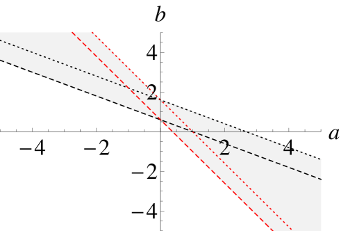
Figure 3: The shaded gray region in the parameter spaces ($a,b$) is consistent with ${\cal O}(1)$ values of Kähler moduli, $T_{\rm min}\leq\langle T_{i}\rangle\leq T_{\rm max}$, where the lower (upper) bounds are chosen, for instance, $T_{\rm min}=0.6$ ($T_{\rm max}=1.6$). The black dashed and dotted lines denote $b=-T_{\rm min}a+T_{\rm min,max}$, while the red dashed and dotted lines denote $b=-T_{\rm max}a+T_{\rm min,max}$, respectively.

As for the parameter spaces ($a,b$) within the shaded region in Fig. 3 corresponding to the ${\cal O}(1)$ values of Kähler moduli, we determine the other $U(1)_{a}$ $a=4,5,\cdots,13$ fluxes so as to achieve the matter contents in the standard model in Eq. (28) and $U(1)_{Y}$ massless conditions (17) as well as (20) and K-theory condition (30).

As a result, within the range $2m_{1}^{i}\in[-11,11]$ and $0.7\leq\langle T_{i}\rangle\leq 1.4$, $i=1,2,3$, the magnetic flux configurations in model $1$ with and without heterotic five-branes are uniquely determined as shown in Tab. 3. Tabs. 4 and 5 also show the magnetic flux configurations in models $2$ and $3$ with and without heterotic five-branes within the range $2m_{1}^{i}\in[-11,11]$ and $0.8\leq\langle T_{i}\rangle\leq 1.3$, $i=1,2,3$, respectively. In the case without five-branes in Tabs. 3, 4 and 5, Eq. (29) is satisfied by the $U(1)$ fluxes themselves. Moreover, the magnetic fluxes in Tabs. 3, 4 and 5 predict the same values of gauge couplings at the string scale, because only $m_{1}^{i}$ and $m_{2}^{i}$ appear in the non-universal terms of $SU(2)_{L}$ and $SU(3)_{C}$ gauge couplings.

Finally, the Figs. 4, 5 and 6 show the values of Kähler moduli and volume of three-tori ${\rm Vol(M)}=\langle T_{1}T_{2}T_{3}\rangle$ as a function of $\langle T_{1}\rangle$ in models $1$, $2$ and $3$, respectively. The ${\cal O}(1)$ values of Kähler moduli in Figs. 4, 5 and 6 are consistent with the experimental values of gauge couplings in the SM and MSSM. Similarly, we can analyze a wider region of $T_{\rm min}<\langle T_{i}\rangle<T_{\rm max}$ with larger $T_{\rm max}$ and smaller $T_{\rm min}$. For example, for $0.3<\langle T_{i}\rangle<3.0$, there are many models consistent with the experimental results of gauge couplings in the SM and MSSM.

Magnetic fluxes	Without five-branes	With five-branes
$(2m_{1}^{1},2m_{1}^{2},2m_{1}^{3})$	(1,-3,-1)	(1,-3,-1)
$(2m_{2}^{1},2m_{2}^{2},2m_{2}^{3})$	(7,-1,1)	(7,-1,1)
$(2m_{3}^{1},2m_{3}^{2},2m_{3}^{3})$	(0,0,0)	(0,0,0)
$(2m_{4}^{1},2m_{4}^{2},2m_{4}^{3})$	(-5,-1,5)	(-5,-5,1)
$(2m_{5}^{1},2m_{5}^{2},2m_{5}^{3})$	(3,1,1)	(1,1,1)
$(2m_{6}^{1},2m_{6}^{2},2m_{6}^{3})$	(3,1,1)	(1,1,1)
$(2m_{7}^{1},2m_{7}^{2},2m_{7}^{3})$	(3,1,1)	(1,1,1)
$(2m_{8}^{1},2m_{8}^{2},2m_{8}^{3})$	(3,1,1)	(1,1,1)

Table 3: The magnetic flux configurations in model $1$ with and without five-branes.

Magnetic fluxes	Without five-branes	With five-branes
$(2m_{1}^{1},2m_{1}^{2},2m_{1}^{3})$	(-3,-1,-1)	(-3,-1,-1)
$(2m_{2}^{1},2m_{2}^{2},2m_{2}^{3})$	(-9,-3,1)	(-9,-3,1)
$(2m_{3}^{1},2m_{3}^{2},2m_{3}^{3})$	(0,0,0)	(0,0,0)
$(2m_{4}^{1},2m_{4}^{2},2m_{4}^{3})$	(11,-1,1)	(9,-1,1)
$(2m_{5}^{1},2m_{5}^{2},2m_{5}^{3})$	(11,1,1)	(9,-1,1)
$(2m_{6}^{1},2m_{6}^{2},2m_{6}^{3})$	(5,-3,-1)	(9,-1,1)
$(2m_{7}^{1},2m_{7}^{2},2m_{7}^{3})$	(9,-1,1)	(9,-1,1)
$(2m_{8}^{1},2m_{8}^{2},2m_{8}^{3})$	(11,-3,-1)	(9,-1,1)

Table 4: The magnetic flux configurations in model $2$ with and without five-branes.

Magnetic fluxes	Without five-branes	With five-branes
$(2m_{1}^{1},2m_{1}^{2},2m_{1}^{3})$	(1,1,11)	(1,1,11)
$(2m_{2}^{1},2m_{2}^{2},2m_{2}^{3})$	(7,-1,9)	(7,-1,9)
$(2m_{3}^{1},2m_{3}^{2},2m_{3}^{3})$	(0,0,0)	(0,0,0)
$(2m_{4}^{1},2m_{4}^{2},2m_{4}^{3})$	(-5,-1,-7)	(-5,-1,-7)
$(2m_{5}^{1},2m_{5}^{2},2m_{5}^{3})$	(-5,-1,-7)	(-5,-1,-7)
$(2m_{6}^{1},2m_{6}^{2},2m_{6}^{3})$	(-5,-1,-7)	(-5,-1,-7)
$(2m_{7}^{1},2m_{7}^{2},2m_{7}^{3})$	(7,1,-23)	(7,1,-3)
$(2m_{8}^{1},2m_{8}^{2},2m_{8}^{3})$	(9,-1,-9)	(7,1,-3)

Table 5: The magnetic flux configurations in model $3$ with and without five-branes.

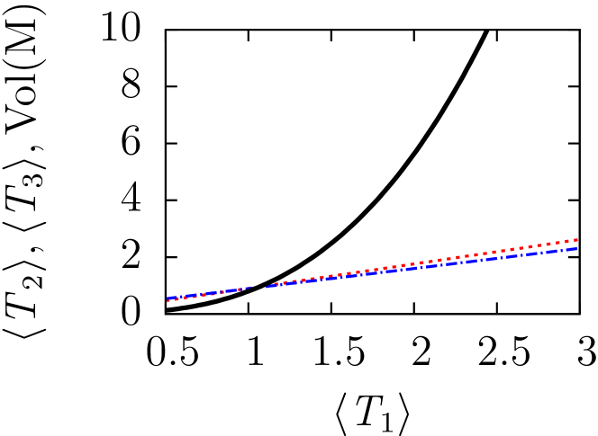
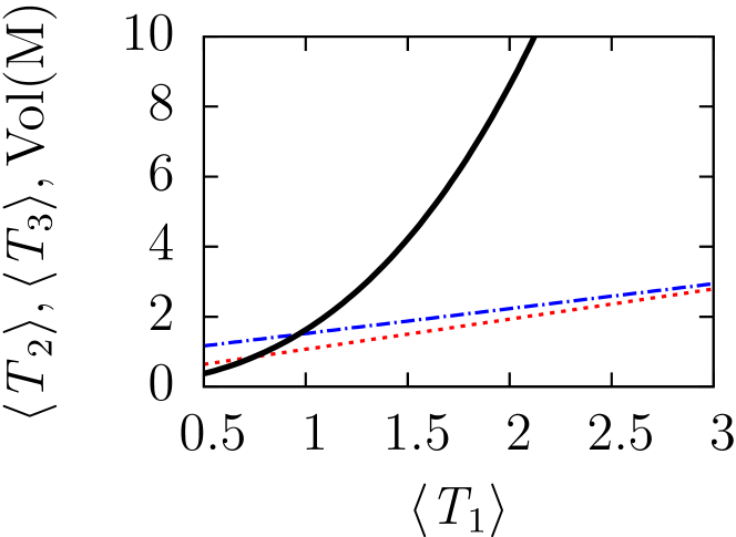
Figure 4: The VEVs of moduli, $\langle T_{2}\rangle$ (red dashed curve), $\langle T_{3}\rangle$ (blue dotdashed curve) and the volume of three-tori ${\rm Vol(M)}=\langle T_{1}T_{2}T_{3}\rangle$ (black thick curve) as a function of $\langle T_{1}\rangle$ in model $1$. The left and right panels show those of SM and MSSM, respectively.

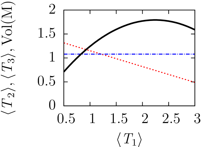
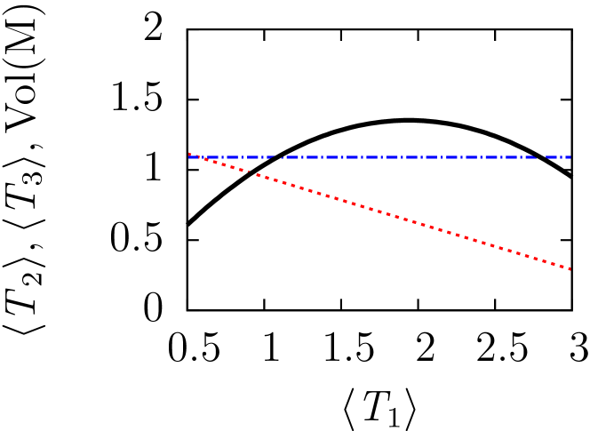
Figure 5: The VEVs of moduli, $\langle T_{2}\rangle$ (red dashed curve), $\langle T_{3}\rangle$ (blue dotdashed curve) and the volume of three-tori ${\rm Vol(M)}=\langle T_{1}T_{2}T_{3}\rangle$ (black thick curve) as a function of $\langle T_{1}\rangle$ in model $2$. The left and right panels show those of SM and MSSM, respectively.

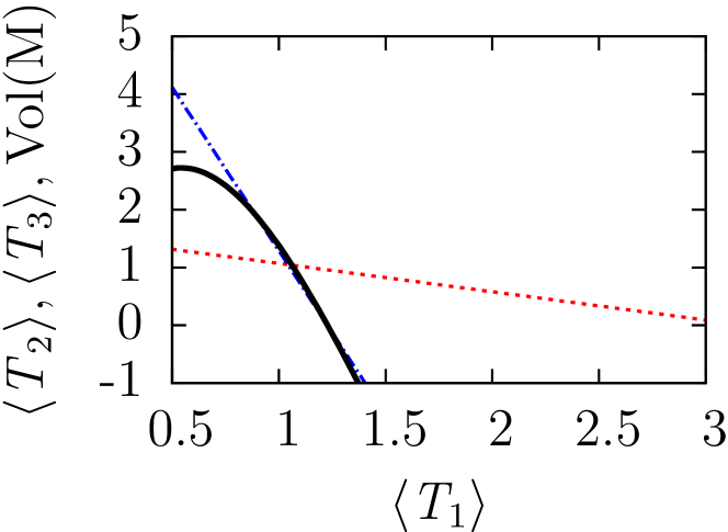
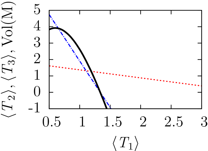
Figure 6: The VEVs of moduli, $\langle T_{2}\rangle$ (red dashed curve), $\langle T_{3}\rangle$ (blue dotdashed curve) and the volume of three-tori ${\rm Vol(M)}=\langle T_{1}T_{2}T_{3}\rangle$ (black thick curve) as a function of $\langle T_{1}\rangle$ in model $3$. The left and right panels show those of SM and MSSM, respectively.

5 Conclusion

We have studied on $SO(32)$ heterotic models with $U(1)$ magnetic fluxes, which have the gauge symmetry including $SU(3)_{C}\times SU(2)_{L}\times U(1)_{Y}$ and three chiral generations of quarks and leptons as well as vector-like matter fields. In contrast to $E_{8}\times E_{8}$ heterotic string theory, there is the non-universality among the gauge couplings of standard model at the string scale and they depend on magnetic fluxes as well as the VEVs of dilaton and Kähler moduli. Although there are several approaches to realize the gauge couplings consistent with their experimental values, they require the large stringy threshold corrections by employing the large field values of Kähler moduli [3, 4, 5] which implies the large string coupling at the vacuum. In this paper, we have considered the two SUSY breaking scenarios. One of them is that the SUSY is broken at the string scale, whereas the other model is the TeV SUSY breaking scenario. In both scenarios, it was found that certain explicit models can lead to the gauge couplings consistent with the experimental values even if the values of Kähler moduli are of order unity. Thus, we have constructed the realistic models from both viewpoints of massless spectra and the gauge couplings.

What is important for a next study would be Yukawa couplings. The zero-mode profiles of quarks and leptons as well as higgs fields are non-trivial because of introducing magnetic fluxes. That would lead to non-trivial Yukawa matrices.. Also, in Ref. [11], it was shown that the models with $N=9$ have $SU(3)$ flavor symmetry. Such a flavor symmetry might be useful to realize the realistic values of fermion masses and mixing angles. We would study this issue elsewhere.

So far, we have taken the dilaton and Kähler moduli VEVs as free parameters in order to obtain the gauge couplings consistent with the experimental values. It is also next issue to study moduli stabilization at proper values of them.

Acknowledgement

H. A. was supported in part by the Grant-in-Aid for Scientific Research No. 25800158 from the Ministry of Education, Culture, Sports, Science and Technology (MEXT) in Japan. T. K. was supported in part by the Grant-in-Aid for Scientific Research No. 25400252 from the MEXT in Japan. H. O. was supported in part by a Grant-in-Aid for JSPS Fellows No. 26-7296.

References

- [1] P. H. Ginsparg, Phys. Lett. B 197, 139 (1987).
- [2] V. S. Kaplunovsky, Nucl. Phys. B 307, 145 (1988) [Erratum-ibid. B 382, 436 (1992)] [hep-th/9205068].
- [3] L. J. Dixon, V. Kaplunovsky and J. Louis, Nucl. Phys. B 355, 649 (1991).
- [4] I. Antoniadis, K. S. Narain and T. R. Taylor, Phys. Lett. B 267, 37 (1991).
- [5] J. P. Derendinger, S. Ferrara, C. Kounnas and F. Zwirner, Nucl. Phys. B 372, 145 (1992).
- [6] L. E. Ibanez, D. Lust and G. G. Ross, Phys. Lett. B 272, 251 (1991) [hep-th/9109053]; L. E. Ibanez and D. Lust, Nucl. Phys. B 382, 305 (1992) [hep-th/9202046].
- [7] H. Kawabe, T. Kobayashi and N. Ohtsubo, Nucl. Phys. B 434, 210 (1995) [hep-ph/9405420]; T. Kobayashi, Int. J. Mod. Phys. A 10, 1393 (1995) [hep-ph/9406238]; R. Altendorfer and T. Kobayashi, Int. J. Mod. Phys. A 11, 903 (1996) [hep-ph/9503388].
- [8] D. Bailin and A. Love, arXiv:1412.7327 [hep-th].
- [9] R. Blumenhagen, D. Lust and S. Stieberger, JHEP 0307, 036 (2003) [hep-th/0305146].
- [10] Y. Hamada, T. Kobayashi and S. Uemura, arXiv:1409.2740 [hep-th].
- [11] H. Abe, T. Kobayashi, H. Otsuka and Y. Takano, arXiv:1503.06770 [hep-th].
- [12] K. S. Choi, T. Kobayashi, R. Maruyama, M. Murata, Y. Nakai, H. Ohki and M. Sakai, Eur. Phys. J. C 67, 273 (2010) [arXiv:0908.0395 [hep-ph]]; T. Kobayashi, R. Maruyama, M. Murata, H. Ohki and M. Sakai, JHEP 1005, 050 (2010) [arXiv:1002.2828 [hep-ph]].
- [13] R. Blumenhagen, G. Honecker and T. Weigand, JHEP 0506 (2005) 020 [hep-th/0504232]; JHEP 0508 (2005) 009 [hep-th/0507041].
- [14] J. Polchinski, String theory. Vol. 2: Superstring theory and beyond. Cambridge University Press, Cambridge,UK, (1998).
- [15] T. Weigand, Fortsch. Phys. 54 (2006) 963.
- [16] E. Witten, Nucl. Phys. B 460 (1996) 541 [hep-th/9511030]; M. J. Duff, R. Minasian and E. Witten, Nucl. Phys. B 465 (1996) 413 [hep-th/9601036]; G. Aldazabal, A. Font, L. E. Ibanez, A. M. Uranga and G. Violero, Nucl. Phys. B 519 (1998) 239 [hep-th/9706158].
- [17] M. B. Green, J. H. Schwarz and P. C. West, Nucl. Phys. B 254, 327 (1985).
- [18] L. E. Ibanez and H. P. Nilles, Phys. Lett. B 169 (1986) 354.
- [19] R. Blumenhagen, S. Moster and T. Weigand, Nucl. Phys. B 751 (2006) 186 [hep-th/0603015].
- [20] E. Witten, Phys. Lett. B 149 (1984) 351.
- [21] E. Witten, JHEP 9812, 019 (1998) [hep-th/9810188].
- [22] A. M. Uranga, Nucl. Phys. B 598, 225 (2001) [hep-th/0011048].
- [23] K. A. Olive et al. [Particle Data Group Collaboration], Chin. Phys. C 38 (2014) 090001.
- [24] D. Cremades, L. E. Ibanez and F. Marchesano, JHEP 0405 (2004) 079 [hep-th/0404229].
- [25] H. Abe, K. S. Choi, T. Kobayashi and H. Ohki, Nucl. Phys. B 814, 265 (2009) [arXiv:0812.3534 [hep-th]]; H. Abe, T. Kobayashi, H. Ohki, A. Oikawa and K. Sumita, Nucl. Phys. B 870, 30 (2013) [arXiv:1211.4317 [hep-ph]]; H. Abe, T. Kobayashi, K. Sumita and Y. Tatsuta, Phys. Rev. D 90, no. 10, 105006 (2014) [arXiv:1405.5012 [hep-ph]].