A Shock Model Based Approach to Network Reliability

Abstract

We consider a network consisting of $n$ components (links or nodes) and assume that the network has two states, up and down. We further suppose that the network is subject to shocks that appear according to a counting process and that each shock may lead to the component failures. Under some assumptions on the shock occurrences, we present a new variant of the notion of signature which we call it t-signature. Then t-signature based mixture representations for the reliability function of the network are obtained. Several stochastic properties of the network lifetime are investigated. In particular, under the assumption that the number of failures at each shock follows a binomial distribution and the process of shocks is non-homogeneous Poisson process, explicit form of the network reliability is derived and its aging properties are explored. Several examples are also provided.

Keywords: signature, fatal shocks, counting process, nonhomogeneous Poisson process, two-state networks, stochastic ordering.

1 Introduction

Networks include a wide variety of real-life systems in communication, industry, software engineering, etc. A network is defined to be a collection of nodes (vertices) and links (edges) in which some particular nodes are called terminals. For instance, nodes can be considered as road intersections, telecommunications switches, servers, and computers; and examples of links can be telecommunication fiber, railways, copper cable, wireless channels, etc.

According to the existing literature, a network can be modeled by the triplet ${\bf N}=(V,E,T)$, in which $V$ shows the node set, where we assume $|V|=m$, $E$ stands for link set, with $|E|=n$, and $T\subseteq V$ is a set of all terminals. When all terminals of the network are connected to each other, the network is called $T-$connected. We assume that the components (links or nodes) of a network are subject to failure, where the failure of the components may occur according to a stochastic mechanism. A link failure means that the link is obliterated and a node failure means that all links incident to that node are erased. Assuming that the network has two states up, and down, the failure of the components may result in the change of the state of the network.

In reliability engineering literature, several approaches are proposed to assess the reliability of a network. An approach, to study the reliability of a network with $n$ components, is based on the assumption that the components of the network have statistically independent and identically distributed (i.i.d.) lifetimes $X_{1},X_{2},\dots,X_{n}$, and the network has a lifetime $T$ which is a function of $X_{1},\dots,X_{n}$. An important concept in this approach is the notion of signature that is presented in the following definition; see [17] and [9].

Definition 1.

Assume that $\pi=(e_{i_{1}},e_{i_{2}},\ldots,e_{i_{n}})$ is a permutation of the network components numbers. Suppose that all components in this permutation are up. We move along the permutation, from left to right, and turn the state of each component from up to down state. Under the assumption that all permutations are equally likely, the signature vector of the network is defined as ${\bf s}=(s_{1},...,s_{n})$ where

$$s_{i}={n_{i}}/{n!},\qquad i=1,\dots,n$$

where $n_{i}$ is the number of permutations in which the failure of $i$th component cause the state of the network changes to a down state. In other words, $s_{i}$ is the probability that the lifetime of the network equals the $i$th ordered lifetimes among $X_{i}$’s, i.e., $s_{i}=P(T=X_{i:n}),$ where $X_{i:n}$ is the $i$th order statistic among the random variables $X_{1},X_{2},\dots,X_{n}$.

The signature vector depends on both the structure of the network and how to define its states. However, it does not depend on the real random mechanism of the component failures. Under this setting, the reliability of the network lifetime $T$, at time $t>0$, can be represented as

$$P(T>t)=\sum_{i=1}^{n}s_{i}P(X_{i:n}>t),$$ (1)

see [18]. In recent years, a large number of research works are reported in the literature investigating different properties of the reliability function (1). We refer, among others, to [18]-[24] and references therein.

Another approach, in assessing the reliability of a network, is recently proposed by Gertsbakh and Shpungin [9]. These authors consider a network with $n$ components, and assume that the component failures appear according to a renewal process $\{N(t),t\geq 0\}$ defined as a sequence of i.i.d. non-negative random variables (r.v.s) $Y_{1},Y_{2},...,Y_{k},\dots$. The random variable $N(t)$ shows the number of components that fail in the network on interval $[0,t]$, and the failures in $\{N(t),t\geq 0\}$ appear at the instants $S_{k}=\sum_{i=1}^{k}{Y_{i}},\ \ k=1,2,\dots$. Under the assumption that all orders of component failures are equally likely, the reliability function of the network lifetime $T$ can be represented as

$$P(T>t)=\sum_{i=1}^{n}\bar{S}_{i}P(N(t)=i),\quad t>0,$$ (2)

where $\bar{S}_{i}=\sum_{k=i+1}^{n}{s_{k}},$. Motivated by this, under the assumption that the failure of the network components occur according to a counting process, Zarezadeh and Asadi [22] investigated various properties of the model in (2) based on different scenarios. Zarezadeh et al. [23] studied stochastic properties of dynamic reliability of networks under the assumption that the components fail according to a nonhomogeneous Poisson process (NHPP).

The aim of the present study is to give new models for the reliability of the network under the assumption that the components of the network are subject to shocks. We consider a two-state network and assume that the network is subject to shocks that appear according to a counting process. We further assume that each shock may lead to component failure and consequently the network finally fails by one of the arriving shocks. The reset of the paper is organized as follows: In Section 2, we obtain the mixture representations for the reliability of the network lifetime. For this purpose, a new variant of the notion of signature, call it t-signature, is introduced which allows us to assume that at same time more that one component failure may occur. We then compare the t-signature based reliability of two different networks under various assumptions. In Section 3, we assume that the number of failed components in each shock are conditionally distributed as binomial distribution. Under this condition, mixture representations for the reliability function of the network are obtained and stochastic and aging properties of the network lifetime are investigated. In particular, we show that when the shocks arrive according to a non-homogeneous Poisson process (NHPP) and the arrival time of the first shock has increasing hazard rate average (IHRA), then the distribution of the network lifetime is IHRA. Section 4 is devoted to the reliability of the network under fatal shocks. It is assumed that at time of occurrence of a shock at least one component of the network fails. Under this assumption a mixture representation for the network reliability is obtained based on a new variant of the notion of signature.

2 Network reliability under shock models

In this section, we assume that the network is subject to shocks that appear according to a counting process. In reality, this may happen as a result of a sequence of heavy road accidents, floods, earthquakes, fires etc. We explore the reliability of the network where each shock may lead to the failure of the network components. Before doing so, we define a variant of the concept of signature which avoids the restriction of not allowing the ties. To be more precise, let $X_{1},...,X_{n}$ be i.i.d random variables representing the component lifetimes of the network. One of the assumptions that is necessary to define the notion of signature is that there do not exist ties between $X_{1},\dots,X_{n}$, i.e. $P(X_{i}=X_{j})=0$ for every $i\neq j$ (see, for example, [20]). However, in real life situation, this is possible that more than one component may fail at each time instant, i.e. ties may exist between $X_{1},\dots,X_{n}$. For example when the network is under shock, each shock may results the failure of more that one component at the same time. Under this assumption, in the sequel, we define a variant of the notion of signature. First let us define the discrete random variable $M$ as the minimum number of components that their failures cause the network failure. Obviously $M$ takes values on $\{1,2,\dots,n\}$. Suppose further that $n^{*}$ is the number of ways that the components fail in the network and $n_{i}$ is the number of ways of the order of component failures in which $M=i$. Assuming that all the number of ways of the order of component failures are equally likely, we define the ”tie signature” (t-signature) vector associated to the network as ${\bf s}^{\tau}=(s_{1}^{\tau},\dots,s_{n}^{\tau})$ where

$$s^{\tau}_{i}=\frac{n_{i}}{n^{*}},\qquad i=1,...,n.$$

It should be noted that t-signature, similar to the concept of signature, depends only on the structure of the network and does not depend on the random mechanism of the component failures.

In the following example, we compute the t-signature vector for a simple network.

Example 1.

Consider a network with $3$ links and $3$ nodes depicted in Figure 1. The links are subjected to failure and nodes $a$ and $c$ are considered as terminals. We assume that the network is functioning if and only if terminals are connected.

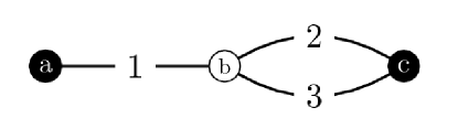
Figure 1: Network with $3$ links and $3$ nodes.

Let $\pi$ denote the order of link failures in the network . All possible $\pi$ and the associated $M$ are presented in Table 1, where the numbers in the braces indicate that the corresponding links failed at the same time. Hence, $n^{*}=13$ and the elements of the t-signature are calculated as

Table 1: All ways of order of links failures

$\pi$	$M$	$\pi$	$M$	$\pi$	$M$
(1,2,3)	1	({1,3},2)	1	({1,2,3})	1
(1,3,2)	1	({2,3},1)	2
(2,1,3)	2	({1,2},3)	1
(2,3,1)	2	(3,{1,2})	2
(3,1,2)	2	(2,{1,3})	2
(3,2,1)	2	(1,{2,3})	1

$$s_{1}^{\tau}=\frac{6}{13},\qquad s_{2}^{\tau}=\frac{7}{13},\qquad s_{3}^{\tau}=0.$$

It is interesting to note that the signature vector of this network equals ${\bf s}=(\frac{1}{3},\frac{2}{3},0).$

The following lemma gives a formula for computing $n^{*}$.

Lemma 1.

Let a $n$-component network be under shocks. Let $n^{*}$ be the number of ways that the components the network fail under the assumption of ties. Then

$$n^{*}=\sum_{j=1}^{n}\sum_{k=0}^{j}{j\choose k}(-1)^{k}(j-k)^{n}.$$

Proof.

We use the following combinatorial argument: The number of ways to put $n$ distinct objects into $m$ distinct boxes, $n>m$, such that every box contains at least one object is

$$\sum_{k=0}^{m}{m\choose k}(-1)^{k}(m-k)^{n}.$$

Let $J$ be the number of shocks such that in occurrence of each one at least one component fails. It is clear that $J$ takes value on $\{1,...,n\}$. If $J=j$, is fixed, the number of ways that the components numbers $\{1,2,...,n\}$ can be under $j$ shocks is the same as the number of ways to put $n$ distinct objects into $j$ distinct boxes such that every box contains at least one object. Thus, summing up over $j$, $j=1,\dots,n$, we get

$$n^{*}=\sum_{j=1}^{n}\sum_{k=0}^{j}{j\choose k}(-1)^{k}(j-k)^{n}.$$

∎

Consider a two-state network with lifetime $T$ which is subject to shocks, where shocks appear according to a counting process, denoted by $\{\xi(t),t>0\}$, at random time instants $\vartheta_{1},\vartheta_{2},\dots$. We assume that each shock may lead to component failures and further assume that the network finally fails by one of these shocks. Let random variable $W_{i}$, $i=1,\dots,n$, denote the number of components that fail at the $i$th shock and $W_{0}\equiv 0$. If $N(t)$ denotes the total number of components that fail up to time $t$, then $N(t)$ takes values on $\{1,2,\dots,n\}$ and

$$N(t)=\sum_{i=0}^{\xi(t)}W_{i}.$$

Under the assumption that the process of occurrence of the shocks is independent of the number of failed components, using the law of total probability, the distribution function of $N(t)$ can be written as

$$P(N(t)\leq x)= \sum_{k=0}^{\infty}P(N(t)\leq x|\xi(t)=k)P(\xi(t)=k)$$

$$= \sum_{k=0}^{\infty}P(\sum_{i=0}^{\xi(t)}W_{i}\leq x|\xi(t)=k)P(\xi(t)=k)$$

$$= \sum_{k=0}^{\infty}H_{k}(x)P(\xi(t)=k),$$ (3)

where $H_{k}(x)$ denotes the distribution function of r.v. $\sum_{i=0}^{k}W_{i}$. By these assumptions, the network fails if $N(t)\geq M$. Hence, the network lifetime can be defined as

$$T\equiv\min_{t>0}\{N(t)\geq M\}$$

and thus, we have $P(T>t)=P(N(t)<M)$. Therefore, using the law of total probability and the fact that the total number of components that fail up to time $t$ is independent of the t-signature, we get

$$P(T>t)= P(N(t)<M)$$

$$= \sum_{i=1}^{n}P(M=i)P(N(t)\leq i-1)$$

$$= \sum_{i=1}^{n}s_{i}^{\tau}P(N(t)\leq i-1).$$ (4)

Let $\bar{S}_{j}^{\tau}=\sum_{i=j+1}^{n}s_{i}^{\tau}$, then using (2) and (2), we have

$$P(T>t)= \sum_{i=1}^{n}s_{i}^{\tau}\sum_{k=0}^{\infty}H_{k}(i-1)P(\xi(t)=k)$$

$$= \sum_{k=0}^{\infty}\beta_{k,n}P(\xi(t)=k),$$ (5)

where, for $k=0,1,\dots$

$$\beta_{k,n}= \sum_{i=1}^{n}s_{i}^{\tau}H_{k}(i-1)$$

$$= \sum_{j=0}^{n-1}\bar{S}_{j}^{\tau}P(\sum_{i=0}^{k}W_{i}=j).$$ (6)

In the following proposition some properties of $\beta_{k,n}$ are investigated.

Proposition 1.

Let $\vartheta_{1},\vartheta_{2},...$ be the epoch times corresponding to $\{\xi(t),t>0\}$. Then

$$\beta_{k,n}=P(T>\vartheta_{k}),$$

and as a function of $k$, $\beta_{k,n}$ is a survival function with probability mass function ${\bf b}_{n}=(b_{1,n},b_{2,n},...)$, where $b_{k,n}=P(T=\vartheta_{k}).$

Proof.

We have

$$P(T>\vartheta_{k}) =\sum_{m=1}^{n}P(T>\vartheta_{k}|M=m)P(M=m)$$

$$=\sum_{m=1}^{n}s_{m}^{\tau}P(\sum_{i=1}^{k}W_{i}<m|M=m)$$

$$=\sum_{m=1}^{n}s_{m}^{\tau}P(\sum_{i=1}^{k}W_{i}<m)$$

$$=\sum_{m=1}^{n}s_{m}^{\tau}H_{k}(m-1)=\beta_{k,n},$$ (7)

where the first equality follows from the fact that the lifetime of network is more than the arrival time of the $k$th shock if and only if the number of failed components in the time of $k$th shock is less than $m$ and the second equality follows because the random variable $M$ is independent of $W_{1},W_{2},\dots.$ Since $\vartheta_{0}\equiv 0$, and the network fails finally with one of the shocks, we have

$$\beta_{0,n}=1,\qquad\lim_{k\rightarrow\infty}\beta_{k,n}=0.$$

On the other hand, since $\{T>\vartheta_{k+1}\}\subseteq\{T>\vartheta_{k}\}$, we get $\beta_{k+1}\leq\beta_{k}$ and hence $\beta_{k,n}$ is decreasing in $k$. Thus $\beta_{k,n}$, as a function of $k$, $k=0,1,\dots$, has properties of a discrete survival function. Let ${\bf b}_{n}=(b_{1,n},b_{2,n},...)$ be the probability mass function corresponding to $\beta_{k,n}$. That is, $b_{k,n}=\beta_{k-1,n}-\beta_{k,n}$. Then, based on (2), we have

$$b_{k,n} =P(T>\vartheta_{k-1})-P(T>\vartheta_{k})=P(T=\vartheta_{k}).$$

∎

From Proposition 1, the $k$th element in ${\bf b}_{n}$, $b_{k,n}$, denotes the probability that the network fails at the time of occurrence of the $k$th shock, $\vartheta_{k}$. We call, throughout the paper, the vector ${\bf b}_{n}$ as the vector of shock t-signature (ST-signature) of the network.

In the following, we show that the reliability function of the network lifetime can be represented as the reliability functions of epoch times $\vartheta_{i}$. For the counting process $\{\xi(t),t>0\}$, it is known that $\{\xi(t)=k\}$ if and only if $\{\vartheta_{k}\leq t<\vartheta_{k+1}\}$ where $\vartheta_{0}\equiv 0$. Using this fact, we have

$$P(T>t)= \sum_{k=0}^{\infty}\beta_{k,n}P(\xi(t)=k)$$

$$= \sum_{k=0}^{\infty}\beta_{k,n}P(\vartheta_{k}\leq t<\vartheta_{k+1})$$

$$= \sum_{k=0}^{\infty}\beta_{k,n}\left(P(\vartheta_{k+1}>t)-P(\vartheta_{k}>t)\right)$$

$$= \sum_{k=1}^{\infty}\beta_{k-1,n}P(\vartheta_{k}>t)-\sum_{k=1}^{\infty}\beta_{k,n}P(\vartheta_{k}>t)$$

$$= \sum_{k=1}^{\infty}b_{k,n}P(\vartheta_{k}>t).$$ (8)

Remark 1.

The model in (5), which arises in reliability theory, is known as the damage shock model (see [2], p. 92). Let a device be subject to shocks appearing randomly over time. Assuming that the device has a probability $\bar{P}(k)$ of surviving the first $k$ shocks, $k=0,1,...$, and $N(t)$ denotes the number of shocks that the device is subject to in the interval $[0,t]$, then the reliability of the device, $\bar{H}(t)$, at time $t$ is

$$\bar{H}(t)=\sum_{k=0}^{\infty}P(N(t)=k)\bar{P}(k),\quad t\geq 0.$$

Various properties of this model have been explored by different authors; see, for example, [3]-[16].

The hazard (failure) rate of a random variable $X$ or its distribution $F$ with density function $f$ is defined by $\lambda_{F}(x)={f(x)}/{\bar{F}(x)}$, where $\bar{F}=1-F$ is the survival function of $X$. The distribution function $F$ is said to be increasing hazard rate (IHR) if ${\bar{F}(t+x)}/{\bar{F}(t)}$ is decreasing in $t$ whenever $x>0$. From representation (8), the hazard rate of the network can be written as

$$\lambda(t)=\sum_{k=1}^{\infty}p_{k,n}(t)\lambda_{k}(t),$$

where $\lambda_{k}(t)$ is the hazard rate of $\vartheta_{k}$ and

$$p_{k,n}(t)=\frac{b_{k,n}P(\vartheta_{k}>t)}{\sum_{j=1}^{\infty}b_{j,n}P(\vartheta_{j}>t)}.$$

It is interesting to note that $p_{k,n}(t)$ can be written as $p_{k}(t)=P(T=\vartheta_{k}|T>t).$ This is true because

$$P(T=\vartheta_{k}|T>t) =\frac{P(T>t|T=\vartheta_{k})P(T=\vartheta_{k})}{P(T>t)}$$

$$=\frac{b_{k,n}P(\vartheta_{k}>t)}{\sum_{j=1}^{\infty}b_{j,n}P(\vartheta_{j}>t)}=p_{k,n}(t),$$

where the second equality follows from the fact that $\{\vartheta_{k}>t\}$ and $\{T=\vartheta_{k}\}$ are independent.

In the following, we make some stochastic comparisons between the performance of two networks, where the components of the networks are subject to failure according to different or same counting processes. We first use the following ordering definitions.

Definition 2.

Let $X$ and $Y$ be two random variables with survival functions $\bar{F}$ and $\bar{G}$ having density functions $f$ and $g$.

• $X$ or $F$ is said to be stochastically less than or equal to $Y$ or $G$, denoted by $X\leq_{st}Y$ or $F\leq_{st}G$, if $\bar{F}(x)\leq\bar{G}(x)$ for all $x$.

• $X$ or $F$ is said to be less than or equal to a random variable $Y$ or $G$ in hazard rate order, denoted by $X\leq_{hr}Y$ or $F\leq_{hr}G$, if $\dfrac{\bar{G}(x)}{\bar{F}(x)}$ increases in $x$.

• $X$ or $F$ is said to be less than or equal to a random variable $Y$ or $G$ in likelihood ratio order, denoted by $X\leq_{lr}Y$ or $F\leq_{lr}G$, if $\dfrac{g(x)}{f(x)}$ is an increasing function of $x$.

We have now the following theorem.

Theorem 1.

Consider two networks consisting of $n_{1}$ and $n_{2}$ components and lifetimes $T_{1}$ and $T_{2}$, respectively. Suppose that the components of the $i$th network are subject to shocks which appear according to counting process $\{\xi_{i}(t),t\geq 0\}$, $i=1,2$. Let the ${\bf b}^{(i)}_{n_{i}}=(b^{(i)}_{1,n_{i}},b^{(i)}_{2,n_{i}},...)$, $i=1,2$ denote the ST-signature of the $i$th network. If $\xi_{1}(t)\geq_{st}\xi_{2}(t)$ and ${\bf b}^{(1)}_{n_{1}}\leq_{st}{\bf b}^{(2)}_{n_{2}}$ then $T_{1}\leq_{st}T_{2}$.

Proof.

Take $\beta_{k,n_{i}}^{(i)}=\sum_{j=k+1}^{\infty}b_{j,n_{i}}^{(i)}$, $i=1,2$. Then, using (5), we have

$$P(T_{1}>t) =\sum_{k=0}^{\infty}\beta^{(1)}_{k,n_{1}}P(\xi_{1}(t)=k)$$

$$\leq\sum_{k=0}^{\infty}\beta^{(1)}_{k,n_{1}}P(\xi_{2}(t)=k)$$

$$\leq\sum_{k=0}^{\infty}\beta^{(2)}_{k,n_{2}}P(\xi_{2}(t)=k)=P(T_{2}>t),$$

where the first inequality follows from the facts that $\beta_{k,n_{i}}$, $i=1,2$ is decreasing in $k$ and the assumption $\xi_{1}(t)\geq_{st}\xi_{2}(t)$. The second inequality follows from the assumption that ${\bf b}^{(1)}_{n_{1}}\leq_{st}{\bf b}^{(2)}_{n_{2}}$. ∎

Corollary 1.

In Theorem 1, assume that the components of the two networks are subject to failure by shocks appear according to renewal processes $\{\xi_{1}(t),t\geq 0\}$ and $\{\xi_{2}(t),t\geq 0\}$, respectively. Let $X_{i,j}$, $i=1,2$, $j=1,2,...$, denote the time between the $(j-1)$th and $j$th shocks in the $i$th network. Then the result of the theorem remains valid if we replace the condition $\xi_{1}(t)\geq_{st}\xi_{2}(t)$ with $X_{1,1}\leq_{st}X_{2,1}$.

Proof.

Let $\vartheta_{i,k}=\sum_{j=1}^{k}X_{i,j},i=1,2,k=1,2,...$. Using Theorem 1.A.3 (b) of [19], the condition $X_{1,1}\leq_{st}X_{2,1}$ implies that $\vartheta_{1,k}\leq_{st}\vartheta_{2,k}$. Now the result follows from Theorem 1 and the fact that for any counting process $\{\xi(t),t\geq 0\}$ with occurrence times $\vartheta_{1},\vartheta_{2},\dots$, we have $\{\vartheta_{n}\leq t\}$ if and only if $\{\xi(t)\geq n\}$. ∎

Before presenting the next theorem, we give the following definition (see, [11]).

Definition 3.

Let $A$ and $B$ be two subsets of the real line. A non-negative function $K$ defined on $A\times B$ is said to be totally positive of order 2, denoted TP₂, if for all $a_{1}<a_{2}$, and $b_{1}<b_{2}$, ($a_{i}\in A$, $b_{i}\in B$, $i=1,2$),

$$K(a_{2},b_{2})K(a_{1},b_{1})-K(a_{1},b_{2})K(a_{2},b_{1})\geq 0.$$

In the next theorem, we show when ST-signature vectors of two networks are hr ordered then the lifetimes of the networks are also ordered in hr ordering.

Theorem 2.

Assume that the assumptions of Theorem 1 are met and that the components of two networks are subject to failure by shocks appear according to the same counting process $\{\xi(t),t\geq 0\}$. If ${\bf b}^{(1)}_{n_{1}}\leq_{hr}{\bf b}^{(2)}_{n_{2}}$ and $P(\xi(t)=k)$ is $TP_{2}$ in $k\in\{0,1,\dots\}$ and $t>0$, then $T_{1}\leq_{hr}T_{2}$.

Proof.

Let $\beta_{k,n_{i}}^{(i)}=\sum_{j=k+1}^{\infty}b_{j,n_{i}}^{(i)},i=1,2$. The assumption ${\bf b}^{(1)}_{n_{1}}\leq_{hr}{\bf b}^{(2)}_{n_{2}}$ implies that ${\beta_{k,n_{2}}^{(2)}}/{\beta_{k,n_{1}}^{(1)}}$ is increasing in $k$. Then, according to Definition 3, it can be concluded that $\beta_{k,n_{i}}^{(i)}$ is $TP_{2}$ in $k\in\{0,1,...\}$ and $i\in{1,2}$. Thus, if $P(\xi(t)=k)$ is $TP_{2}$ in $k\in\{0,1,...\}$ and $t>0$, then from basic decomposition formula (see, [11]), we get

$$P(T_{i}>t)=\sum_{k=1}^{\infty}\beta^{(i)}_{k,n_{i}}P(\xi(t)=k)$$

is $TP_{2}$ in $i\in\{1,2\}$, and $t>0$ which in turn implies that $T_{1}\leq_{hr}T_{2}$. ∎

Remark 2.

In Theorem 1, if we assume that the components of two networks fail by shocks appear according to the same renewal processes based on i.i.d. r.v.s $X_{i},i=1,2,...$, then under the assumption that ${\bf b}^{(1)}_{n_{1}}\leq_{hr}{\bf b}^{(2)}_{n_{2}}$ and that $X_{1}$ has increasing hazard rate, we have $T_{1}\leq_{hr}T_{2}$. This is true because when $X_{1}$ has increasing hazard rate then $\vartheta_{k}\leq_{hr}\vartheta_{k+1},k=1,2,..$ and hence, the required result follows from the representation (8) and Theorem 1.B.14 of [19]. Also if $X_{1}$ has log-concave density function, then $\vartheta_{k}\leq_{lr}\vartheta_{k+1},k=1,2,...$. Thus using Theorem 1.C.17 of [19], if ${\bf b}^{(1)}_{n_{1}}\leq_{lr}{\bf b}^{(2)}_{n_{2}}$ and $X_{1}$ has log-concave density function then $T_{1}\leq_{lr}T_{2}$.

3 A binomial based model

In this section, we consider the shock model is presented in Section 2 and assume that the number of component failures at each shock follows a binomial distribution. Suppose that when a shock arrives each component fails with probability $p$. Assuming that the components fail independent of each other, the number of failed components in the first shock, $W_{1}$, has binomial distribution $b(n,p)$, where $n$ is the number of components in the network. Suppose that, the number of failed components in the $i$th shock, $W_{i}$, $i\geq 2$, depends only on $W_{1},...,W_{i-1}$ through $\sum_{j=1}^{i-1}W_{j}$ and has binomial distribution $b(n_{i},p)$, where $n_{i}=n-\sum_{j=1}^{i-1}W_{j}$. In other words, assume that

$$P(W_{1}=k)={n\choose k}p^{k}q^{n-k},~{}~{}~{}k=0,1,...,n$$ (9)

and for $i\geq 2$,

$$P(W_{i}=k|\sum_{j=1}^{i-1}W_{j}=w)={n-w\choose k}p^{k}q^{n-w-k},~{}~{}~{}k=0,...,n-w,~{}w<n,$$ (10)

where $q=1-p$.

Now we can prove the following lemma.

Lemma 2.

Under the assumptions (9) and (10), we have

$$P(\sum_{i=1}^{n}W_{i}=j)={n\choose j}(1-q^{k})^{j}q^{k(n-j)},~{}~{}~{}j=0,...,n,~{}k=1,2,\dots.$$

Proof.

We prove the lemma by induction. For $k=1$ the result is true by relation (9). Assume that the result is true for $k=m$. That is

$$P(\sum_{i=1}^{m}W_{i}=j)={n\choose j}(1-q^{m})^{j}q^{m(n-j)}.$$

Then, for $k=m+1$, we get

$$P(\sum_{i=1}^{m+1}W_{i}=j) = \sum_{k=0}^{j}P(W_{m+1}=j-k|\sum_{i=1}^{m}W_{i}=k)P(\sum_{i=1}^{m}W_{i}=k)$$

$$= \sum_{k=0}^{j}{n-k\choose j-k}{n\choose k}p^{j-k}q^{n-j}(1-q^{m})^{k}q^{m(n-k)}$$

$$= \sum_{k=0}^{j}{n-k\choose j-k}{n\choose k}p^{j-k}q^{n-j}p^{k}(\sum_{i=0}^{m-1}q^{i})^{k}q^{m(n-k)}$$

$$= {n\choose j}p^{j}q^{n(m+1)-j}\sum_{k=0}^{j}{j\choose k}(\frac{\sum_{i=0}^{m-1}q^{i}}{q^{m}})^{k}$$

$$= {n\choose j}p^{j}q^{n(m+1)-j}(\frac{\sum_{i=0}^{m}q^{i}}{q^{m}})^{j}$$

$$= {n\choose j}(1-q^{m+1})^{j}q^{(m+1)(n-j)},$$

which is the required result. ∎

Now, based on the model given in (5), the reliability of the network at time $t$ is

$$P(T>t)=\sum_{k=0}^{\infty}\beta^{*}_{k,n}P(\xi(t)=k),$$ (11)

where $\beta^{*}_{0,n}=1$, and for $k=1,2,...$

$$\beta^{*}_{k,n} =\sum_{j=0}^{n-1}{\bar{S}}_{j}^{\tau}{n\choose j}(1-q^{k})^{j}q^{k(n-j)}$$ (12)

$$=\sum_{i=1}^{n}s_{i}^{\tau}\sum_{j=0}^{i-1}{n\choose j}(1-q^{k})^{j}q^{k(n-j)}$$

$$=\sum_{m=1}^{n}\sum_{j=n-m}^{n-1}{\bar{S}}_{j}^{\tau}{n\choose j}{j\choose n-m}(-1)^{j-n+m}q^{km}.$$

From representation (8), we have

$$P(T>t)=\sum_{k=1}^{\infty}b^{*}_{k,n}P(\vartheta_{k}>t),$$

where $b^{*}_{k,n}=(\beta^{*}_{k-1,n}-\beta^{*}_{k,n})$.

In the following, we concentrate on a special case where the shocks appear as a nonhomogeneous Poisson process (NHPP). Recall that a counting process $\{\xi(t),t\geq 0\}$ is called a NHPP if the survival function of arrival time $\vartheta_{k}$ of the $k$th event is

$$\bar{G}_{k}(t)=\sum_{x=0}^{k-1}\frac{[\Lambda(t)]^{x}}{x!}e^{-\Lambda(t)},\ \quad t>0,\ k=1,2,...,$$

where $\Lambda(t)=E(N(t))=-\log\bar{G}(t)$, and $\bar{G}(t)$ is the reliability function of the time to the first event. The function $\Lambda(t)$ is called the mean value function (m.v.f.). For more details on the properties of NHPP and related processes, one can see, for example, [13].

Let us look at the following example.

Example 2.

Consider a series network consisting of $n$ components. Suppose that the network is subject to shocks which appear according to a NHPP with m.v.f. $\Lambda(t)=-\log\bar{G}(t)$. Then under model (11) and noting that the t-signature of a series network is ${\bf s}^{\tau}=(1,0,0,\dots,0)$, we can easily see that

$$\beta^{*}_{k,n}=q^{kn},\qquad k=0,1,2,\dots.$$

Hence, the reliability of series network is given by

$$P(T>t)= \sum_{k=0}^{\infty}q^{kn}P(\xi(t)=k)$$

$$= \sum_{k=0}^{\infty}q^{kn}e^{-\Lambda(t)}\frac{\left(\Lambda(t)\right)^{k}}{k!}$$

$$= e^{-\Lambda(t)}\sum_{k=0}^{\infty}\frac{\left(q^{n}\Lambda(t)\right)^{k}}{k!}$$

$$= e^{-\Lambda(t)\left(1-q^{n}\right)}$$

$$= (\bar{G}(t))^{1-q^{n}}$$

Note that if $n$, the number of components of the network, gets large then the reliability of the network tends to $\bar{G}(t)$.

In the sequel, we explore some aging properties of the network lifetime. First, recall that a distribution $F$ is said to be increasing hazard rate average (IHRA) if $\left(\bar{F}(t)\right)^{1/t}$ is decreasing in $t>0$. It is well known that the IHR property implies the IHRA (see [2]).

We have the following lemma.

Lemma 3.

$\beta^{*}_{k,n}$ is IHRA.

Proof.

In order to prove the result, we must show $(\beta^{*}_{k,n})^{\frac{1}{k}}$ is decreasing in $k$ for $k=1,2,\dots$. Note that $\beta_{k,n}^{*}$ can be rewritten as

$$\beta_{k,n}^{*}=\sum_{j=1}^{n}s_{j}^{\tau}\int_{1-q^{k}}^{1}\frac{u^{j-1}(1-u)^{n-j}}{B(j,n-j+1)}du,$$ (13)

which is clearly an increasing function of $q^{k}$. It is clear from (12) that $\beta^{*}_{k,n}$ is a static reliability function of a network. If we write $\beta^{*}_{k,n}=h(q^{k})$, where $h$ is the reliability function of the network, then by choosing $\alpha=\frac{k}{k+1}$ in Theorem 2.5 of Section 4 of [2], we conclude that

$$h(q^{(k+1)(\frac{k}{k+1})})\geq h^{\frac{k}{k+1}}(q^{k+1})$$

which is equivalent to say that

$$(\beta^{*}_{k,n})^{\frac{1}{k}}\geq(\beta^{*}_{k+1,n})^{\frac{1}{k+1}}.$$

This completes the proof of the lemma. ∎

The following example shows that, although $\beta^{*}_{k,n}$ is always IHRA, but it is not necessarily IHR.

Example 3.

Consider a bridge network pictured in Figure 2. It can be seen that the t-signature of this network is as ${\bf s}^{\tau}=(0,\frac{77}{270},\frac{154}{270},\frac{39}{270},0)$. In order to show that $\beta^{*}_{k,n}$ is IHR we have to show, based on the definition of IHR distributions, that $\frac{\beta_{k+1}^{*}}{\beta_{k}^{*}}$ is decreasing in $k$.

Figure 2: The bridge network.

Figure 3 shows the plot of $\frac{\beta_{k+1}^{*}}{\beta_{k}^{*}}$ for this network where $q=0.5$. As the plot shows, this ratio is not decreasing for all values of $k$, hence $\beta_{k}^{*}$ is not IHR.

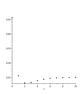
Figure 3: The plot of $\frac{\beta^{*}_{k+1}}{\beta_{k}^{*}}$ for the bridge network.

Theorem 4.1 of [10] implies that if $P(\xi(t)=k)$ is $TP_{2}$ in $t\in(0,\infty)$, and $k\in\{0,1,...\}$ and $(E(a^{\xi(t)}))^{\frac{1}{t}}$ is decreasing in $t$ for $a\in(0,1)$, then based on the fact that $\beta^{*}_{k,n}$ is IHRA we get that $T$ is also IHRA. The following theorem shows that under the condition that $\xi(t)$ is NHPP, the network lifetime $T$ is IHRA if the distribution function of the arrival time of the first shock is IHRA.

Theorem 3.

Consider a network consisting of $n$ components with lifetime $T$. Suppose that the components of the network is subject to failure by shocks that appear according to a NHPP with m.v.f. $\Lambda(t)=-\log\bar{G}(t)$. If $\bar{G}$ is IHRA, then $T$ is IHRA.

Proof.

For $k_{1}\leq k_{2}$,

$$\frac{P(\xi(t)=k_{2})}{P(\xi(t)=k_{1})}=\frac{k_{1}!}{k_{2}!}\left(\Lambda(t)\right)^{k_{2}-k_{1}}$$

is increasing in $t$ and hence $P(\xi(t)=k)$ is TP₂ in $k$ and $t$. On the other hand, for $a\in(0,1)$

$$E(a^{\xi(t)})= \sum_{n=0}^{\infty}a^{n}\frac{(\Lambda(t))^{n}}{n!}e^{-\Lambda(t)}$$

$$= e^{-\Lambda(t)}\sum_{n=0}^{\infty}\frac{(a\Lambda(t))^{n}}{n!}=e^{-{\Lambda(t)}(1-a)}$$

$$= \left(\bar{G}(t)\right)^{1-a}.$$

If $\bar{G}(t)$ is IHRA, then $(G(t))^{\frac{1}{t}}$ is decreasing in $t$ and hence

$$\left(E(a^{\xi(t)})\right)^{\frac{1}{t}}=\left(\bar{G}(t)\right)^{\frac{1-a}{t}}$$

is decreasing in $t$. Hence the result follows from Theorem 4.1 of Gottlieb [10]. ∎

In the next theorem the stochastic relationships between t-signature vectors and the lifetimes of two networks are investigated.

Theorem 4.

Consider two networks with lifetimes $T_{1}$ and $T_{2}$ and t-signature vectors ${\bf s}_{1}^{\tau}=(s_{1,1}^{\tau},...,s_{1,n}^{\tau})$ and ${\bf s}_{2}^{\tau}=(s_{2,1}^{\tau},...,s_{2,n}^{\tau})$, respectively. Suppose that the components of the $i$th network is subject to failure by shocks appear according to NHPP with m.v.f. $\Lambda_{i}(t)=-\log\bar{G}_{i}(t)$, $i=1,2$. Assume that, upon arriving the shocks, the components of the $i$th network fail with probability $p_{i}$, $i=1,2$.

• If $p_{1}\geq p_{2}$, $G_{1}\leq_{st}G_{2}$ and ${\bf s}_{1}^{\tau}\leq_{st}{\bf s}_{2}^{\tau}$ then $T_{1}\leq_{st}T_{2}$.

• If $p_{1}=p_{2}$, $G_{1}=_{st}G_{2}$ and ${\bf s}_{1}^{\tau}\leq_{hr}{\bf s}_{2}^{\tau}$ then $T_{1}\leq_{hr}T_{2}$.

Proof.

Let $\beta_{k,n}^{*(i)}=\sum_{j=k+1}^{\infty}b_{j,n}^{*(i)},$ where $b_{j,n}^{*(i)}$ is the $j$th element of ST-signature associated to the $i$th network and $q_{i}=1-p_{i},~{}i=1,2$.

• Let $\{\xi_{i}(t),t>0\}$ be the NHPP with m.v.f. $\Lambda_{i}(t)=-\log\bar{G}_{i}(t),~{}i=1,2$. Supose that $g_{j,n}(q_{i}^{k})=\int_{1-q_{i}^{k}}^{1}\frac{u^{j-1}(1-u)^{n-j}}{B(j,n-j+1)}du,~{}i=1,2.$ Using (13), it can be seen that $\beta^{*(i)}_{k,n}=\sum_{j=1}^{n}s_{i,j}^{\tau}g_{j,n}(q_{i}^{k})$, where $g_{j,n}(q_{i}^{k})$ is an increasing function of $q_{i}^{k}$. Hence

  $$\beta_{k,n}^{*(1)} =\sum_{j=1}^{n}s_{1,j}^{\tau}g_{j,n}(q_{1}^{k})$$

  $$\leq\sum_{j=1}^{n}s_{2,j}^{\tau}g_{j,n}(q_{1}^{k})$$

  $$\leq\sum_{j=1}^{n}s_{2,j}^{\tau}g_{j,n}(q_{2}^{k})=\beta_{k,n}^{*(2)}$$

  in which the first inequality follows from the fact that ${\bf s}_{1}^{\tau}\leq_{st}{\bf s}_{2}^{\tau}$ and $g_{j,n}(q^{k})$ is increasing in $j$ and second equality follows from the assumption $p_{1}\geq p_{2}$ which implies $g_{j,n}(q_{1}^{k})\leq g_{j,n}(q_{2}^{k})$. Also, $G_{1}\leq_{st}G_{2}$ implies $\xi_{1}(t)\geq_{st}\xi_{2}(t)$. Then the result follows from Theorem 1.

• It is easy to see that ${n\choose j}(1-q_{1}^{k})^{j}q_{1}^{k(n-j)}$ is $TP_{2}$ in $k$ and $j$. Also, ${\bf s}_{1}^{\tau}\leq_{hr}{\bf s}_{2}^{\tau}$ implies that ${\bar{S}}_{i,j}^{\tau}$ is $TP_{2}$ in $i$ and $j$. Therefore from basic decomposition formula (see [11]),

  $$\beta^{*(i)}_{k,n}=\sum_{j=0}^{n-1}{\bar{S}}_{i,j}^{\tau}{n\choose j}(1-q_{1}^{k})^{j}q_{1}^{k(n-j)}$$

  is $TP_{2}$ in $k\in\{0,1,...\}$ and $i\in\{1,2\}$ which implies ${\bf b}_{n}^{*(1)}\leq_{hr}{\bf b}_{n}^{*(2)}$. The proof is complete based on Theorem 2.

∎

Example 4.

Consider again Example 3. Let the network be subject to shocks that appear according to a NHPP with m.v.f. $\Lambda(t)=-\log\bar{G}(t)$ and in each shock, each link fails with probability $0.1$. We are interested in assessing the reliability of the network in the cases where the time to the first shock has either an exponential distribution with a constant hazard rate of $1$ (Exp(1)), or a Weibull distribution with shape parameter $2$ and scale parameter $1$ (W(2,1)), or a linear hazard distribution (L(1,1/2)). The survival functions of these distributions, respectively, are given as

$$\bar{G}_{1}(t)= \exp(-t),\qquad t>0,$$

$$\bar{G}_{2}(t)= \exp(-{t^{2}}),\qquad t>0,$$

$$\bar{G}_{3}(t)= \exp(-t-t^{2}),\qquad t>0.$$

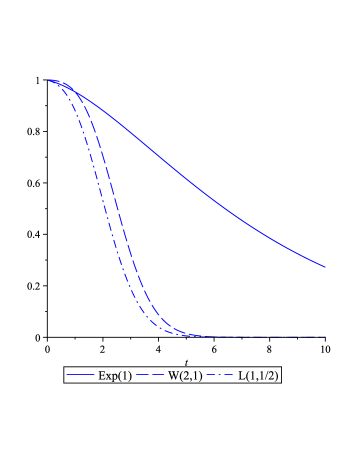
Figure 4: The plot of network reliability in Example 4.

It can be easily shown that L(1,1/2) is stochastically less than both Exp(1) and W(2,1). Hence, as Figure 4 reveals, based on Theorem 4, the reliability of the network for the L(1,1/2) case is less than that of the cases of Exp(1) or W(2,1). It can be easily seen that Exp(1) and W(2,1) are not stochastically ordered. Also, the plot shows that the network lifetimes are not stochastically ordered.

4 Network reliability under fatal shocks

In this section, we assume that each shock is fatal for the network. That is, when a shock arrives it leads to failure of at least one component. Let fatal shocks occur according to a counting process, $\{\zeta(t),t>0\}$, at random time instants $\varrho_{1},\varrho_{2},\dots$. It is clear that the network finally fails by one of the fatal shocks. In order to obtain the reliability function of the network, in such a situation, first we obtain $P(T=\varrho_{i}),~{}i=1,\dots n$. Consider a network consists of $n$ components. It can be shown that the number of ways showing the order of component failures is $n^{*}$ given in Lemma 1. Then, under the assumption that all ways of the order of component failures are equally likely, we have

$$s_{i}^{*}\equiv P(T=\varrho_{i})=\frac{n_{i}}{n^{*}},\quad i=1,\dots n,$$

where $n_{i}$ is the number of ways of the order of component failures in which $i$th fatal shock causes the network fails. It is obvious that $s_{i}^{*}$ just depends on the structure of the network. In the following example, we compute ${\bf s}^{*}=(s_{1}^{*},\dots,s_{n}^{*})$.

Example 5.

Consider again Example 1. Let $\pi$ denote the order of link failures in the network and $r(\pi)$ the shock number that caused the failure of the network. All possible $\pi$ and corresponding $r(\pi)$ have been presented in Table 2. It is clear that

$$s_{1}^{*}=P(T=\varrho_{1})=\frac{7}{13}\qquad s_{2}^{*}=P(T=\varrho_{2})=\frac{6}{13},\qquad s_{3}^{*}=P(T=\varrho_{3})=0.$$

That is, ${\bf s}^{*}=(\frac{7}{13},\frac{6}{13},0)$.

Table 2: All possible $\pi$ and corresponding $r(\pi)$

$\pi$	$r(\pi)$	$\pi$	$r(\pi)$	$\pi$	$r(\pi)$
(1,2,3)	1	({1,3},2)	1	({1,2,3})	1
(1,3,2)	1	({2,3},1)	1
(2,1,3)	2	({1,2},3)	1
(2,3,1)	2	(3,{1,2})	2
(3,1,2)	2	(2,{1,3})	2
(3,2,1)	2	(1,{2,3})	1

From the fact that $s_{i}^{*}$ does not depend on the random mechanism of the component failures, we obtain the reliability function of the network as

$$P(T>t)= \sum_{i=1}^{n}P(T>t|T=\varrho_{i})P(T=\varrho_{i})$$

$$= \sum_{i=1}^{n}s_{i}^{*}P(\varrho_{i}>t|T=\varrho_{i})$$

$$= \sum_{i=1}^{n}s_{i}^{*}P(\varrho_{i}>t).$$ (14)

From the fact that $\zeta(t)=k$ if and only if $\varrho_{k}\leq t<\varrho_{k+1}$, it can be seen that

$$P(T>t)= \sum_{i=0}^{n-1}{\bar{S}}^{*}_{i}P(\zeta(t)=i)$$ (15)

where ${\bar{S}}^{*}_{i}=\sum_{j=i+1}^{n}s^{*}_{j}$.

Remark 3.

It is noted that the representations (4) and (15) are similar to representations (8) and (5), respectively. Hence, the results obtained based on (8) and (5) in Section 2 are valid for the fatal shock model.

Acknowledgement:

M. Asadi s research was carried out in IPM Isfahan branch and was in part supported by a grant from IPM (No. 93620411).

References

- [1] N. Balakrishnan and M. Asadi, “A proposed measure of residual life of live components of a coherent system,” IEEE Transactions on Reliability, vol. 61, no. 1, pp. 41-49, 2012.
- [2] R. E. Barlow and F. Proschan, Statistical Theory of Reliability and Life Testing: Probability Models. Florida State Univ Tallahassee, 1975.
- [3] N. Ebrahimi, “Stochastic properties of a cumulative damage threshold crossing model,” Journal of Applied Probability, vol. 36, no. 3, pp. 720-732, 1999.
- [4] S. Eryilmaz, “On the lifetime distribution of consecutive -out-of-: system,” IEEE Transactions on Reliability, vol. 56, no. 1, pp. 35-39, 2007.
- [5] S. Eryilmaz, “Conditional lifetimes of consecutive -out-of- systems,” IEEE Transactions on Reliability, vol. 59, no. 1, pp. 178-182, 2010.
- [6] S. Eryilmaz, “The number of failed components in a coherent system with exchangeable components,” IEEE Transactions on Reliability, vol. 61, no. 1, pp. 203-207, 2012.
- [7] S. Eryilmaz and B. Mahmoud “Linear -consecutive- , -out-of-: system,” IEEE Transactions on Reliability, vol. 61, no. 3, pp. 787-791, 2012.
- [8] S. Eryilmaz and M. J. Zuo, “Computing and applying the signature of a system with two common failure criteria,” IEEE Transactions on Reliability, vol. 59, no. 3, pp. 576-580, 2010.
- [9] I. Gertsbakh and Y. Shpungin, Network Reliability and Resilience. Springer Briefs, Springer, 2011.
- [10] G. Gottlieb, “Failure distributions of shock models,” Journal of Applied Probability, vol. 17, no. 3, pp. 745-752, 1980.
- [11] S. Karlin, Total Positivity. Vol. 1. Stanford University Press, 1968.
- [12] T. Nakagawa, Shock and Damage Models in Reliability Theory. In: Springer series in reliability engineering, Springer, London, UK, 2007.
- [13] T. Nakagawa, Stochastic Processes: With Applications to Reliability Theory. In: Springer series in reliability engineering, 2011.
- [14] J. Navarro, N. Balakrishnan and F. J. Samaniego, “Mixture reptesentations of residual lifetimes of used systems,” Journal of Applied Probability, vol. 45, pp. 1097-1112, 2008.
- [15] J. Navarro and M. Burkschat, “Coherent systems based on sequential order statistics,” Naval Research Logistics, vol. 58, no. 2, pp. 123-135, 2011.
- [16] F. Pellerey, “Partial orderings under cumulative damage shock models,” Journal of Applied Probability, vol. 25, pp. 939-946, 1993.
- [17] F. J. Samaniego, “On closure of the IFR class under formation of coherent systems,” IEEE Transactions on Reliability, vol. 34, pp. 69-72, 1985.
- [18] F. J. Samaniego, System Signatures and Their Applications in Reliability Engineering. New York, Berlin: Springer, 2007.
- [19] M. Shaked and J. G. Shanthikumar, Stochastic Orders. Springer, 2007.
- [20] F. Spizzichino and J. Navarro, “ Signatures and symmetry properties of coherent systems,“ In Recent Advances in System Reliability, Springer London, pp. 33-48, 2012.
- [21] I. S. Triantafyllou and V. K. Markos, “Signature and IFR preservation of 2-within-consecutive -out-of-: systems,” IEEE Transactions on Reliability, vol. 60, no. 1, pp. 315-322, 2011.
- [22] S. Zarezadeh and M. Asadi, “Network reliability modeling under stochastic process of component failures,” IEEE Transactions on Reliability, vol. 62, no. 4, pp. 917-929, 2013.
- [23] S. Zarezadeh, M. Asadi and N. Balakrishnan, “Dynamic network reliability modeling under nonhomogeneous Poisson processes,” European Journal of Operational Research, vol. 232, pp. 561-571, 2014.
- [24] Z. Zhang and X. Li, “Some new results on stochastic orders and aging properties of coherent systems,” IEEE Transactions on Reliability, vol. 59, no. 4, pp. 718-724, 2010.