The untwisting number of a knot

Abstract.

The unknotting number of a knot is the minimum number of crossings one must change to turn that knot into the unknot. The algebraic unknotting number is the minimum number of crossing changes needed to transform a knot into an Alexander polynomial-one knot. We work with a generalization of unknotting number due to Mathieu-Domergue, which we call the untwisting number. The untwisting number is the minimum number (over all diagrams of a knot) of right- or left-handed twists on even numbers of strands of a knot, with half of the strands oriented in each direction, necessary to transform that knot into the unknot. We show that the algebraic untwisting number is equal to the algebraic unknotting number. However, we also exhibit several families of knots for which the difference between the unknotting and untwisting numbers is arbitrarily large, even when we only allow twists on a fixed number of strands or fewer.

1. Introduction

It is a natural knot-theoretic question to seek to measure “how knotted up” a knot is. One such “knottiness” measure is given by the unknotting number $u(K)$, the minimum number of crossings, taken over all diagrams of $K$, one must change to turn $K$ into the unknot. By a crossing change we shall mean one of the two local moves on a knot diagram given in Figure 1.1.

Figure 1.1. A positive and negative crossing change.

This invariant is quite simple to define but has proven itself very difficult to master. Fifty years ago, Milnor conjectured that the unknotting number for the $(p,q)$-torus knot was $(p-1)(q-1)/2$; only in 1993, in two celebrated papers [KM93, KM95], did Kronheimer and Mrowka prove this conjecture true. Hence, it is desirable to look at variants of unknotting number which may be more tractable. One natural variant (due to Murakami [Mur90]) is the algebraic unknotting number $u_{a}(K)$, the minimum number of crossing changes necessary to turn a given knot into an Alexander polynomial-one knot. Alexander polynomial-one knots are significant because they “look like the unknot” to classical invariants, knot invariants derived from the Seifert matrix. It is obvious that $u_{a}(K)\leq u(K)$ for any knot $K$, and there exist knots such that $u_{a}(K)<u(K)$ (for instance, any nontrivial knot with trivial Alexander polynomial).

In [MD88], Mathieu and Domergue defined another generalization of unknotting number. In [Liv02], Livingston worked with this definition. He described it as follows:

“One can think of performing a crossing change as grabbing two parallel strands of a knot with opposite orientation and giving them one full twist. More generally, one can grab $2k$ parallel strands of $K$ with $k$ of the strands oriented in each direction and give them one full twist.”

Following Livingston, we call such a twist a generalized crossing change. We describe in Section 2.1 how a crossing change may be encoded as a $\pm 1$-surgery on a nullhomologous unknot $U\subset S^{3}-K$ bounding a disk $D$ such that $D\cap K=2$ points. From this perspective, a generalized crossing change is a relaxing of the previous definition to allow $D\cap K=2k$ points for any $k$, provided $\text{lk}(K,U)=0$ (see Fig. 1.2). In particular, any knot can be unknotted by a finite sequence of generalized crossing changes.

Figure 1.2. A right-handed, or positive, generalized crossing change.

One may then naturally define the untwisting number $tu(K)$ to be the minimum length, taken over all diagrams of $K$, of a sequence of generalized crossing changes beginning at $K$ and resulting in the unknot. By $tu_{p}(K)$, we will denote the minimum number of twists on $2p$ or fewer strands needed to unknot $K$; notice that $tu_{1}(K)=u(K)$ and that

$$tu\leq\dots\leq tu_{p+1}\leq tu_{p}\leq\dots\leq tu_{1}=u.$$

The algebraic untwisting number $tu_{a}(K)$ is the minimum number of generalized crossing changes, taken over all diagrams of $K$, needed to transform $K$ into an Alexander polynomial-one knot. It is clear that $tu_{a}(K)\leq tu(K)$ for all knots $K$.

It is natural to ask how $tu(K)$ and $u(K)$ are related. We show that these invariants are “algebraically the same” in the following sense:

Theorem 1.1.

For any knot $K\subset S^{3}$, $tu_{a}(K)=u_{a}(K)$.

Therefore, $tu$ and $u$ cannot be distinguished by classical invariants. By using the Jones polynomial, which is not a classical invariant, we can show that $tu$ and $u$ are not equal in general:

Theorem 1.2.

Let $K$ be the image of $V\subset S^{3}$ in the manifold $M\cong S^{3}$ resulting from $+1$-surgery on the unknot $U\subset S^{3}$ shown in Figure 1.3. Then $tu(K)=1$ but $u(K)>1$.

Figure 1.3. The generalized crossing change for $V\subset S^{3}$ which results in a knot $K\subset S^{3}$ with $tu(K)\neq u(K)$.

Furthermore, using the fact that the absolute value of the Ozsváth-Szabó $\tau$ invariant is a lower bound on unknotting number, we show in Subsection 5.1 that the difference $u-tu_{p}$ can be arbitrarily large, and thus so can the difference $u-tu$. Throughout this paper, $K_{p,q}$ will denote the $(p,q)$-cable of the knot $K$, where $p$ denotes the longitudinal winding and $q$ the meridional winding.

Theorem 1.3.

Let $K$ be a knot in $S^{3}$ such that $u(K)=1$. If $\tau(K)>0$ and $p,q>0$, then

$$u(K_{p,q})-tu_{p}(K_{p,q})\geq p-1.$$

In particular, if we take $q=1$, then $tu_{p}(K_{p,q})=1$, while $u(K_{p,q})\geq p$.

It may seem that the above examples are “cheating” in some sense, as in each of them the number of strands of $K$ passing through the $\pm 1$-framed unknot $U$ in the generalized crossing change diagram is increasing along with $u(K)$. The following theorem shows that $u(K)$ can be arbitrarily larger than $tu(K)$ even when we restrict to doing $q$-generalized crossing changes for any fixed integer $q\geq 1$.

Theorem 1.4.

For any knot $K$ with $u(K)=1$ and $\tau(K)>0$, the infinite family of knots $J_{p}^{q}:=\#^{p}K_{q,1}$ satisfies

$$u(J_{p}^{q})-tu_{q}(J_{p}^{q})\geq p$$

for any integers $p>1,q>0$.

So far, all of the families of knots we have worked with are quite complicated, in the sense that they are $(p,q)$-cables for large $p$ or connected sums of such cables. One may wonder whether it is possible to find a “simpler” knot $K$ for which $tu(K)<u(K)$. One measure of “knot simplicity” is topological sliceness; a knot $K$ is topologically slice if there exists a locally flat disk $D\subset B^{4}$ such that $\partial D=K\subset S^{3}=\partial B^{4}$.

Theorem 1.5.

For any knot $K$ with $\tau(K)>0$, let $D_{+}(K,0)$ denote the positive-clasped, untwisted Whitehead double of $K$. Then the knots $S_{p}^{q}:=\#^{p}(D_{+}(K,0))_{q,1}$ are topologically slice and satisfy

$$u(S_{p}^{q})-tu_{q}(S_{p}^{q})\geq p$$

for all integers $p>0,q>0$.

This paper is organized as follows. First, we will review the operations of Dehn surgery on knots and knot cabling and define the untwisting number more precisely. Next, we will give some background on the Blanchfield form which is necessary to prove that $tu_{a}=u_{a}$. Finally, we will prove that each of the above families of knots give arbitrarily large gaps between $u$ and $tu$.

Convention. In this paper, all manifolds are assumed to be compact, orientable, and connected.

2. Preliminaries

2.1. Dehn surgery

In this section, we will describe the operation of Dehn surgery on knots.

Definition 2.1.

Let $K\subset S^{3}$ be an oriented knot and $U\subset S^{3}$ be an unknot with $\text{lk}(K,U)=0$. Let $W$ be a closed tubular neighborhood of $U$ in $S^{3}$. Let $\lambda$ be a longitude of $W$, and let $\mu$ be a meridian of $W$ such that $\text{lk}(\mu,\lambda)=1$. The $3$-manifold

$$M=(S^{3}-\mathring{W})\bigcup_{h}W,$$

where $h:\partial W\to\partial W$ is a homeomorphism taking a meridian of $W$ onto $\pm\mu+\lambda\subset W$, is the result of $\pm 1$-surgery on $U$, and $U$ is said to be $\pm 1$-framed. In this situation, we define a generalized crossing change diagram for $K$ to be a diagram of the link $K\cup U$ with the number $\pm 1$ written next to $U$, indicating that $U$ is $\pm 1$-framed. Figure 1.3 is an example of a generalized crossing change diagram for the unknot $V$.

In the general case, note that the complement of $\mathring{N}\supset U$ in $S^{3}$ is a solid torus, which we may modify with a meridinal twist. This alters $K$ as follows: if $D$ is a disk bounded by $U$ such that $k$ strands of $K$ pass through $D$ in straight segments, then each of the $k$ straight pieces is replaced by a helix which screws through a neighborhood of $D$ in the right-hand sense (see Fig. 2.1).

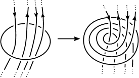
Figure 2.1. A right-handed twist about an unknotted component.

If $U$ is $-1$-framed, the knot obtained by erasing $U$ and twisting the strands of $K$ that pass through $U$ as in Figure 2.1 represents the image of $K$ under the $-1$-surgery on $U$ [Rol76]. If instead $U$ has framing $+1$, the knot obtained by erasing $U$ and giving $K$ a left-handed meridinal twist represents the image of $K$ under the $+1$-surgery on $U$. The process of performing a $\mp$-meridinal twist on the complement of a $\pm 1$-framed unknot $U$, then erasing $U$ from the resulting diagram, is called a blow-down on $U$. The inverse process of introducing an unknotted component $U$ to a surgery diagram consisting of a knot $K$, then performing a $\pm$-meridinal twist on the complement of $U$ it to link it with $K$, is known as a blow-up on $U$ and results in a diagram consisting of $K$ and the $\mp 1$-framed unknot $U$, where $\text{lk}(K,U)=0$.

Figure 2.2. Crossing changes as blow-downs of $\pm 1$-framed unknots.

Now, it can be easily verified that blowing down the $+1$-framed unknot on the left side of Figure 2.2 transforms the crossing labeled $+$ into the crossing labeled $-$. The inverse process of introducing an unknot to the right side of Figure 2.2 and performing a $-$-meridinal twist on its complement yields the positive crossing.

2.2. Untwisting number

We define a $\pm$-generalized crossing change on $K$ as the process of blowing down the $\pm 1$-framed unknot in a generalized crossing change diagram for $K$. In this situation, $K$ must pass through $U$ an even number of times, for otherwise $\text{lk}(K,U)\neq 0$. If at most $2p$ strands of $K$ pass through $U$ in a generalized crossing change diagram, we may call the associated $\pm$-generalized crossing change a $\pm p$-generalized crossing change on $K$.

The result of a $\pm$-generalized crossing change on $K$ is defined to be the image of $K$ under the blow-down. The untwisting number $tu(K)$ of $K$ is the minimum length of a sequence of generalized crossing changes on $K$ such that the result of the sequence is the unknot, where we allow ambient isotopy of the diagram in between generalized crossing changes. Note that by the reasoning on page 58 of [Ada94], this definition is equivalent to taking the minimum length, over all diagrams of $K$, of a sequence of generalized crossing changes beginning with a fixed diagram of $K$ such that the result of the sequence is the unknot, where we do not allow ambient isotopy of the diagram in between generalized crossing changes.

For $p=1,2,3,\dots$, we define the $p$-untwisting number $tu_{p}(K)$ to be the minimum length of a sequence of $\pm p$-generalized crossing changes on $K$ resulting in the unknot, where we allow ambient isotopy of the diagram in between generalized crossing changes.

It follows immediately that we have the chain of inequalities

(2.1) $$tu(K)\leq\dots\leq tu_{p+1}(K)\leq tu_{p}(K)\leq\dots\leq tu_{2}(K)\leq tu_{1}(K)=u(K).$$

2.3. Cabling

In this section, we define satellite and cable knots.

Definition 2.2.

A closed subset $X$ of a solid torus $V\cong S^{1}\times D^{2}$ is called geometrically essential in $V$ if $X$ intersects every PL meridinal disk in $V$.

Let $P\subset V\subset S^{3}$ be a knot which is geometrically essential in an unknotted solid torus $V$. Let $C\subset S^{3}$ be another knot and let $V_{1}$ be a tubular neighborhood of $C$ in $S^{3}$. Let $h\colon V\to V_{1}$ be a homeomorphism and let $K$ be $h(P)$. Then $P$ is called the pattern for the knot $K$, $C$ is the companion of $K$, and $K$ is called a satellite of $C$ with pattern $P$, or just a satellite knot for short.

If the homeomorphism $h$ takes the preferred longitude and meridian of $V$, respectively, to the preferred longitude and meridian of $V_{1}$, then $h$ is said to be faithful. If $P$ is the $(p,q)$-torus knot just under $\partial V$ and $h$ is faithful, then $K$ is called the $(p,q)$-cable based on $C$, denoted $C_{p,q}$, or simply a cable knot.

Throughout this paper, we will denote the $(p,q)$-torus knot by $U_{p,q}$ since it is the $(p,q)$-cable of the unknot $U$.

2.4. The Blanchfield form

Let $K\subset S^{3}$ be a knot. By $\Lambda$ we shall denote the ring $\mathbb{Z}[t^{\pm 1}]$, and by $\Omega$ we will denote the field $\mathbb{Q}(t)$.

2.4.1. Twisted homology, cohomology groups, and Poincaré duality

Following [BF14], let $X$ be a manifold with infinite cyclic first homology, and fix a choice of isomorphism of $H_{1}(X)$ with the infinite cyclic group generated by the indeterminate $t$. Let $\pi\colon\widetilde{X}\to X$ be the infinite cyclic cover of $X$. Given a submanifold $Y$ of $X$, let $\widetilde{Y}=\pi^{-1}(Y)$. Since $\mathbb{Z}$ is the deck transformation group of $\widetilde{X}$, $\Lambda$ acts on the relative chain group $C_{\ast}(\widetilde{X},\widetilde{Y};\mathbb{Z})$. If $N$ is any $\Lambda$-module, we may define

$$H^{\ast}(X,Y;N):=H_{\ast}(\text{Hom}_{\Lambda}(C_{\ast}(\widetilde{X},\widetilde{Y};\mathbb{Z}),N))$$

and

$$H_{\ast}(X,Y;N):=H_{\ast}(\overline{C_{\ast}(\widetilde{X},\widetilde{Y};\mathbb{Z}})\otimes_{\Lambda}N).$$

Here, if $H$ is any $\Lambda$-module, $\overline{H}$ denotes the module with the involuted $\Lambda$-structure: multiplication by $p(t)\in\Lambda$ in $\overline{H}$ is the same as multiplication by $p(t^{-1})$ in $H$. When $Y=\emptyset$, we just write $H_{\ast}(X;N)$ or $H^{\ast}(X;N)$.

Since $\Omega:=\mathbb{Q}(t)$ is flat over $\Lambda$, we have isomorphisms $H_{\ast}(X,Y;\Omega)\cong H_{\ast}(X,Y;\Lambda)\otimes_{\Lambda}\Omega$ and $H^{\ast}(X,Y;\Omega)\cong H^{\ast}(X,Y;\Lambda)\otimes_{\Lambda}\Omega$. If $X$ is an $n$-manifold, and $N$ is a $\Lambda$-module, Poincaré duality gives $\Lambda$-module isomorphisms

$$H_{i}(X,\partial X;N)\cong H^{n-i}(X;N).$$

2.4.2. The Blanchfield form

As above, let $\Lambda=\mathbb{Z}[t,t^{-1}]$ and $\Omega=\mathbb{Q}(t)$. Let $A$ be an $n\times n$ invertible hermitian matrix with entries in $\Lambda$. We define $\lambda(A)$ to be the pairing

$$\lambda(A)\colon\Lambda^{n}/A\Lambda^{n}\times\Lambda^{n}/A\Lambda^{n}\to\Omega/\Lambda$$

sending the pair of column vectors $(a,b)$ to $\bar{a}^{t}A^{-1}b$. Note that $\lambda(A)$ is a nonsingular, hermitian pairing.

Let $X(K)=S^{3}-N(K)$ denote the exterior of $K$. Consider the following sequence of maps:

$$\Phi\colon H_{1}(X(K);\Lambda) \xrightarrow{\pi_{\ast}} H_{1}(X(K),\partial X(K);\Lambda)$$

$$\xrightarrow{PD} H^{2}(X(K);\Lambda)\xleftarrow{\delta}H^{1}(X(K);\Omega/\Lambda)$$

$$\xrightarrow{ev} \overline{\text{Hom}_{\lambda}(H_{1}(X(K);\Lambda),\Omega/\Lambda)}.$$

Here $\pi_{\ast}$ is induced by the quotient map $C(X)\to C(X)/C(\partial X)$, $PD$ is the Poincaré duality map, $\delta$ is from the long exact sequence in cohomology obtained from the coefficients $0\to\Lambda\to\Omega\to\Omega/\Lambda\to 0$, and $ev$ is the Kronecker evaluation map. It is well-known (see [Hil12, Section 2] for details) that $\pi_{\ast}$ and $\delta$ are isomorphisms, $PD$ is the Poincaré duality isomorphism, and $ev$ is also an isomorphism by the universal coefficient spectral sequence (see [Lev77, Theorem 2.3] for details on the universal coefficient spectral sequence). Thus, the above maps define a nonsingular pairing

$$\lambda(K)\colon H_{1}(X(K);\Lambda)\times H_{1}(X(K);\Lambda) \to \Omega/\Lambda$$

$$(a,b) \mapsto \Phi(a)(b),$$

called the Blanchfield pairing of $K$. It is well-known that this pairing is hermitian.

Now, let $V$ be any $2k\times 2k$ matrix which is $S$-equivalent to a Seifert matrix for $K$. Recall that $V-V^{T}$ is antisymmetric with determinant $\pm 1$. It is well-known that, perhaps after replacing $V$ by $PVP^{T}$ for some $P\in GL_{2k}(\mathbb{Z})$,

(2.2) $$V-V^{T}=\begin{pmatrix}0&-I_{k}\\ I_{k}&0\end{pmatrix},$$

where $I_{k}$ denotes the $k\times k$ identity matrix. We define $A_{K}(t)$ to be the matrix

$$\begin{pmatrix}(1-t^{-1})^{-1}I_{k}&0\\ 0&I_{k}\end{pmatrix}V\begin{pmatrix}I_{k}&0\\ 0&(1-t)I_{k}\end{pmatrix}+\begin{pmatrix}I_{k}&0\\ 0&(1-t^{-1})I_{k}\end{pmatrix}V^{T}\begin{pmatrix}(1-t)^{-1}I_{k}&0\\ 0&I_{k}\end{pmatrix}.$$

Using (2.2), we can write

$$V=\begin{pmatrix}B&C+I\\ C^{T}&D\end{pmatrix}.$$

One may then compute, as in the proof of [BF15, Lemma 2.2], that

$$A_{K}(1)=\begin{pmatrix}B&-I_{k}\\ -I_{k}&0\end{pmatrix}.$$

Thus, the matrix $A_{K}(t)$ is a Hermitian matrix defined over $\Lambda$, and $\det(A_{K}(1))=(-1)^{k}$.

Proposition 2.3.

[BF15, Proposition 2.1] Let $K$ be a knot and $A_{K}(t)$ be as above. Then $\lambda(A_{K}(t))$ is isometric as a sesquilinear form to $\lambda(K)$.

2.5. The twisted intersection pairing

Let $W$ be a topological $4$-manifold with boundary $M$ such that $\pi_{1}(W)=\mathbb{Z}$. Consider the maps

$$H_{2}(W;\Lambda)\xrightarrow{\pi_{\ast}}H_{2}(W,M;\Lambda)\xrightarrow{PD}H^{2}(W;\Lambda)\xrightarrow{ev}\overline{\text{Hom}_{\Lambda}(H_{2}(W;\Lambda),\Lambda)},$$

where the first map is induced by the quotient, the second map is Poincaré duality, and the third map is the Kronecker evaluation map. The second and third maps are obviously isomorphisms, and the first map is an isomorphism by the long exact sequence of the pair $(W,M)$. Hence this composition defines a pairing

$$H_{2}(W;\Lambda)\times H_{2}(W;\Lambda)\to\Lambda$$

which we call the twisted intersection pairing on $W$.

3. Algebraic untwisting number equals algebraic unknotting number

Our proof that $tu_{a}(K)=u_{a}(K)$ generalizes the work of Borodzik and Friedl in [BF14, BF15]. Following [BF14], define a knot invariant $n(K)$ to be the minimum size of a square Hermitian matrix $A(t)$ over $\mathbb{Z}[t^{\pm 1}]$ such that $\lambda(A)$ is isometric to $\lambda(K)$ and $A(1)$ is congruent over $\mathbb{Z}$ to a diagonal matrix which has only $\pm 1$ entries. Borodzik and Friedl showed that $u_{a}(K)=n(K)$. Since $tu_{a}(K)\leq u_{a}(K)$, it is obvious that $tu_{a}(K)\leq n(K)$ as well. After stating Borodzik and Friedl’s results, we will show that $n(K)\leq tu_{a}(K)$, hence $tu_{a}(K)=n(K)=u_{a}(K)$ for all knots $K$. In fact, we will show something stronger.

Theorem 3.1.

Let $K\subset S^{3}$ be a knot. For every algebraic unknotting sequence for $K$ with $u_{+}$ positive crossing changes and $u_{-}$ negative crossing changes, there exists an algebraic untwisting sequence for $K$ with $u_{+}$ positive generalized crossing changes and $u_{-}$ negative generalized crossing changes. In particular, $u_{a}(K)=tu_{a}(K)$.

In order to prove Theorem 3.1, we must first recall some notation and results used by Borodzik and Friedl in [BF15]. The main theorem of [BF15] implies that $n(K)\leq u_{a}(K)$:

Theorem 3.2.

[BF15, Theorem 1.1] Let $K$ be a knot which can be changed into an Alexander polynomial-one knot by a sequence of $u_{+}$ positive crossing changes and $u_{-}$ negative crossing changes. Then there exists a hermitian matrix $A(t)$ of size $u_{+}+u_{-}$ over $\Lambda$ such that

1. $\lambda(A(t))$ is isometric to $\lambda(K)$;

2. $A(1)$ is a diagonal matrix such that $u_{+}$ diagonal entries are equal to $-1$ and $u_{-}$ diagonal entries are equal to $1$.

In particular, $n(K)\leq u_{a}(K)$.

We need one definition:

Definition 3.3.

Let $K$ be a knot and $M(K)$ the result of $0$-surgery on $K$. A $4$-manifold $W$ tamely cobounds $M(K)$ if:

1. $\partial W=M(K)$;

2. the inclusion induced map $H_{1}(M(K);\mathbb{Z})\to H_{1}(W;\mathbb{Z})$ is an isomorphism;

3. $\pi_{1}(W)=\mathbb{Z}$.

If, in addition, the intersection form on $H_{2}(W;\mathbb{Z})$ is diagonalizable, we say that $W$ strictly cobounds $M(K)$.

The following theorem of Borodzik-Friedl is also needed:

Theorem 3.4.

[BF15, Theorem 2.6] Let $K$ be a knot and let $W$ be a topological $4$-manifold which tamely cobounds $M(K)$. Then $H_{2}(W;\Lambda)$ is free of rank $b_{2}(W)$. Moreover, if $B$ is an integral matrix representing the ordinary intersection pairing of $W$, then there exists a basis $\mathcal{B}$ for $H_{2}(W;\Lambda)$ such that the matrix $A(t)$ representing the twisted intersection pairing with respect to $\mathcal{B}$ satisfies

1. $\lambda(A(t))$ is isometric to $\lambda(K)$;

2. $A(1)=B$.

We generalize Theorem 3.2 as follows:

Theorem 3.5.

Let $K$ be a knot which can be changed into an Alexander polynomial-one knot by a sequence of $u_{+}$ positive and $u_{-}$ negative generalized crossing changes. Then there exists a hermitian matrix of size $u_{+}+u_{-}$ over $\Lambda$ with the following two properties:

1. $\lambda(A(t))$ is isometric to $\lambda(K)$;

2. $A(1)$ is a diagonal matrix such that $u_{+}$ diagonal entries are equal to $-1$ and $u_{-}$ diagonal entries are equal to $1$.

In particular, $n(K)\leq tu_{a}(K)$.

The proof of Theorem 3.5 is quite similar to the proof of Theorem 3.2. By Theorem 3.4, in order to prove Theorem 3.5, we only need to show the following proposition.

Proposition 3.6.

Let $K$ be a knot such that $u_{+}$ positive generalized crossing changes and $u_{-}$ negative generalized crossing changes turn $K$ into an Alexander polynomial-one knot. Then there exists an oriented topological $4$-manifold $W$ which strictly cobounds $M(K)$. Moreover, the intersection pairing on $H_{2}(W;\mathbb{Z})$ is represented by a diagonal matrix of size $u_{+}+u_{-}$ such that $u_{+}$ entries are equal to $-1$ and $u_{-}$ entries are equal to $+1$.

Proof.

Let $K$ be a knot such that $u_{+}$ positive generalized crossing changes and $u_{-}$ negative generalized crossing changes turn $K$ into an Alexander polynomial-one knot $J$. We write $s=u_{+}+u_{-}$ and $n_{i}=-1$ for $i=1,\dots,u_{+}$ and $n_{i}=1$ for $i=u_{+}+1,\dots,u_{+}+u_{-}$. Then there exist simple closed curves $c_{1},\dots,c_{s}$ in $S^{3}-N(J)$ such that

1. $c_{1}\cup\dots\cup c_{s}$ is the unlink in $S^{3}$;

2. the linking numbers $\text{lk}(c_{i},K)$ are zero for all $i$;

3. the image of $J$ under the $n_{i}$-surgeries is the knot $K$.

Note that the curves $c_{1},\dots,c_{s}$ lie in $S^{3}-N(J)$, hence we can view them as lying in $M(J)$. The manifold $M(K)$ is then the result of $n_{i}$-surgery on all the $c_{i}\subset M(J)$, where $i=1,\dots,s$.

Since $J$ is a knot with trivial Alexander polynomial, by Freedman’s theorem [FQ14] $J$ is topologically slice and there exists a locally flat slice disk $D\subset B^{4}$ for $J$ such that $\pi_{1}(B^{4}-D)=\mathbb{Z}$. Let $X:=B^{4}-N(D)$. Then $X$ is an oriented topological $4$-manifold such that

1. $\partial X\cong M(J)$ as oriented manifolds;

2. $\pi_{1}(X)\cong\mathbb{Z}$;

3. the inclusion induced map $H_{1}(M(J);\mathbb{Z})\to H_{1}(X;\mathbb{Z})$ is an isomorphism;

4. $H_{2}(X;\mathbb{Z})=0$.

Let $W$ be the $4$-manifold which is obtained by adding $2$-handles along $c_{1},\dots,c_{s}\subset M(J)$ with framings $n_{1},\dots,n_{s}$ to $X$. Then $\partial W\cong M(K)$ as oriented manifolds. From now on, we write $M:=M(K)$. Since the curves $c_{1},\dots,c_{s}$ are nullhomologous, the map $H_{1}(M;\mathbb{Z})\to H_{1}(W;\mathbb{Z})$ is an isomorphism and $\pi_{1}(W)\cong\mathbb{Z}$. It thus remains to prove the following lemma:

Lemma 3.7.

The ordinary intersection pairing on $W$ is represented by a diagonal matrix of size $s=u_{+}+u_{-}$ with $u_{+}$ diagonal entries equal to $-1$ and $u_{-}$ diagonal entries equal to $1$.

Recall that the curves $c_{1},\dots,c_{s}$ form the unlink in $S^{3}$ and that the linking numbers $\text{lk}(c_{i},J)$ are zero. Therefore, the curves $c_{1},\dots,c_{s}$ are also nullhomologous in $M(J)$. Thus we can now find disjoint surfaces $F_{1},\dots,F_{s}$ in $M(J)\times[0,1]$ such that $\partial F_{i}=c_{i}\times\{1\}$. By adding the cores of the $2$-handles attached to the $c_{i}$, we obtain closed surfaces $C_{1},\dots,C_{s}$ in $W$. It is clear that $C_{i}\cdot C_{j}=0$ for $i\neq j$ and $C_{i}\cdot C_{i}=n_{i}$.

We argue using Mayer-Vietoris that the surfaces $C_{1},\dots,C_{s}$ present a basis for $H_{2}(W;\mathbb{Z})$. Write $W:=X\cup H$ where $H\cong\sqcup_{i=1}^{s}(B^{2}\times B^{2})$ is the set of $2$-handles attached to $c_{1},\dots,c_{s}$. Then write $Y:=X\cap H$, so that

$$Y=\sqcup_{i=1}^{s}N(c_{i})\cong\sqcup_{i=1}^{s}(S^{1}\times D^{2}).$$

We have the Mayer-Vietoris sequence

$$\dots\to H_{2}(X)\oplus H_{2}(H)\xrightarrow{\psi_{\ast}}H_{2}(W)\xrightarrow{\partial_{\ast}}H_{1}(Y)\xrightarrow{\phi_{\ast}}H_{1}(X)\oplus H_{1}(H)\xrightarrow{\psi_{\ast}}H_{1}(W)\to 0.$$

Now, since $H_{1}(Y)$ is generated by all the $S^{1}$-factors, or the longitudes $c_{1},\dots,c_{s}$, and $H_{1}(H)=H_{2}(H)=H_{2}(X)=0$, the sequence becomes

$$0\to H_{2}(W)\xrightarrow{\partial_{\ast}}\langle c_{1},\dots,c_{s}\rangle\xrightarrow{i_{\ast}}H_{1}(X)\xrightarrow{\psi_{\ast}}H_{1}(W)\to 0.$$

From e.g. [Liv93, Lemma 8.12], we have

Lemma 3.8.

Suppose that for some knot $K$ in $S^{3}$, there is a locally flat surface $F$ in $B^{4}$ with $F\cap S^{3}=\partial F\cap S^{3}=K$. Then the inclusion map induces an isomorphism $H_{1}(S^{3}-K)\to H_{1}(B^{4}-F)\cong\mathbb{Z}$.

In our case, the inclusion $S^{3}-K\hookrightarrow X$ induces an isomorphism $H_{1}(S^{3}-K)\to H_{1}(X)$. Since $i_{\ast}$ is induced by inclusion and the longitudes $c_{1},\dots,c_{s}$ are nullhomologous in $S^{3}-K$, hence in $X$, $i_{\ast}$ must be the zero map. Hence $\partial_{\ast}$ is an isomorphism $H_{2}(W)\cong H_{1}(Y)$, and $H_{2}(W)=\langle C_{1},\dots,C_{s}\rangle$.

In particular, the intersection matrix on $W$ with respect to this basis is given by $(C_{i}\cdot C_{j})$, i.e. it is a diagonal matrix such that $u_{+}$ diagonal entries are equal to $-1$ and $u_{-}$ diagonal entries are equal to $+1$. This concludes the proof of Lemma 3.7. Proposition 3.6 follows. Together with Theorem 3.4, this completes the proof of Theorem 3.5. ∎

We have shown that, for every untwisting sequence for $K$ with $u_{+}$ positive generalized crossing changes and $u_{-}$ negative generalized crossing changes, there exists a hermitian matrix $A(t)$ of size $u_{+}+u_{-}$ such that $\lambda(A(t))$ is isometric to $\lambda(K)$ and $A(1)$ is diagonal with $u_{+}$ entries equal to $-1$ and $u_{-}$ entries equal to $1$. Borodzik and Friedl [BF14] have already shown that, for every hermitian matrix $A(t)$ representing $\lambda(K)$ such that $A(1)$ is diagonal with $u_{+}$ $-1$’s and $u_{-}$ $+1$’s, there exists an algebraic unknotting sequence for $K$ consisting of $u_{+}$ positive and $u_{-}$ negative crossing changes. Theorem 3.1 follows.

4. Untwisting Number Does Not Equal Unknotting Number

Although the algebraic versions of $tu$ and $u$ are equal, $tu\neq u$ in general. We use a result of Miyazawa [Miy98] to give our first example of a knot $K$ with $tu(K)=1$ but $u(K)>1$.

Theorem 4.1.

Let $K$ be the knot resulting from blowing down the $(+1)$-framed unknot $U\subset S^{3}\setminus V$ in Figure 1.3. Then $tu(K)=1$ but $u(K)>1$.

From this point forward, we will denote the signature of any knot $K$ by $\sigma(K)$. In order to analyze the unknotting number of $K$, we will use the following theorem:

Theorem 4.2.

[Miy98] If $u(K)=1$ and $\sigma(K)=\pm 2$, then

$$V_{K}^{(1)}(-1)\equiv 24a_{4}(K)-\frac{\sigma(K)}{8}(\det K+1)(\det K+5)\text{ (mod 48)}$$

where $V_{K}^{(1)}$ denotes the first derivative of the Jones polynomial of $K$ and $a_{4}$ is the coefficient of $z^{4}$ in the Conway polynomial $\nabla_{K}(z)=\sum_{n=0}^{\infty}a_{2n}(K)z^{2n}$.

We compute using the Mathematica package KnotTheory [mat] that $\sigma(K)=2$, hence Theorem 4.2 applies. We also compute using the KnotTheory package that the Jones polynomial $V_{K}(q)$ for our knot $K$ is

$$V_{K}(q)=q-q^{2}+2q^{3}-q^{4}+q^{6}-q^{7}+q^{8}-q^{9}-q^{12}+q^{13},$$

hence $V_{K}^{(1)}(-1)=8$. The Conway polynomial of $K$ is computed to be

$$\nabla_{K}(z)=\sum_{n=0}^{\infty}a_{2n}(K)z^{2n}=1+z^{2}$$

(hence $a_{4}=0$), and the determinant of $K$ is $3$. In our case, the right-hand side of the congruence in Theorem 4.2 becomes

$$0-\frac{1}{4}(4)(8)=-8$$

and $8\not\equiv-8$ (mod $48$). Hence $K$ cannot have unknotting number one, although it was constructed to have untwisting number one. Note that this also shows Miyazawa’s Jones polynomial criterion does not extend to untwisting number-one knots.

5. Arbitrarily large gaps between unknotting and untwisting numbers

5.1. Arbitrarily large gaps between $u$ and $tu_{p}$

Now that we have shown that there exists a knot $K$ with $tu(K)<u(K)$, it is natural to ask how large the difference $u(K)-tu(K)$ can be. Recall that the $(p,q)$-cable of a knot $K$ is denoted $K_{p,q}$; we denote the $(p,q)$-torus knot as $U_{p,q}$, the $(p,q)$-cable of the unknot. The knots we will be working with are $(p,q)$-cables of knots $K$ with $u(K)=1$ and $\tau(K)>0$, where $p,q>0$.

In order to get a lower bound on $u(K_{p,q})$ for such knots, we compute $\tau(K_{p,q})$ for all $p,q$. For cables of alternating (or more generally, “homologically thin”) knots such as the trefoil, Petkova [Pet13] gives a formula for computing $\tau$. However, since we will later compute $\tau$ for cables of non-alternating knots, we use a more general method of computing $\tau(K_{p,q})$ using the $\epsilon$-invariant $\epsilon(K)\in\{-1,0,1\}$ introduced by Hom in [Hom14]:

Theorem 5.1.

[Hom14] Let $K\subset S^{3}$.

1. If $\epsilon(K)=1$, then $\tau(K_{p,q})=p\tau(K)+\frac{(p-1)(q-1)}{2}$.

2. If $\epsilon(K)=-1$, then $\tau(K_{p,q})=p\tau(K)+\frac{(p-1)(q+1)}{2}$.

3. If $\epsilon(K)=0$, then $\tau(K)=0$ and $\tau(K_{p,q})=\tau(U_{p,q})=\begin{cases}\frac{(p-1)(q+1)}{2},&q<0\\ \frac{(p-1)(q-1)}{2},&q>0.\end{cases}$

We note the following property of $\tau$:

Theorem 5.2.

[OS03] For the $(p,q)$-torus knot $U_{p,q}$ with $p,q>0$, $\tau$ equals the $3$-sphere genus of $U_{p,q}$, denoted $g(U_{p,q})$:

$$\tau(U_{p,q})=g(U_{p,q})=\frac{(p-1)(q-1)}{2}.$$

We also need the following proposition of Hom:

Proposition 5.3.

[Hom14] Let $K\subset S^{3}$ be a knot. If $|\tau(K)|=g(K)$, then $\epsilon(K)=\text{sgn }\tau(K)$.

Theorem 5.4.

Let $K$ be a knot in $S^{3}$ with unknotting number one. If $\tau(K)>0$ and $p,q>0$, then

$$u(K_{p,q})-tu_{p}(K_{p,q})\geq p-1.$$

In particular, $tu_{p}(K_{p,1})=1$, while $u(K_{p,1})\geq p$.

Proof.

Let $V$ be the unknot that results from performing the unknotting crossing change on $K$. Consider a generalized crossing change diagram for $V$ together with the $\pm 1$-framed surgery curve $U$ that transforms $V$ back into $K$. Then take the $(p,q)$-cable $V_{p,q}$ of $V$ in this diagram, leaving $U$ alone. The resulting $V_{p,q}$ is the $(p,q)$-torus knot before performing the $\pm 1$-surgery, but the image of $V$ under $\pm 1$-surgery on $U$ is $K$, hence the image of $V_{p,q}$ under the $\pm 1$-surgery on $U$ is $K_{p,q}$. Therefore, blowing down the surgery curve $U$ (through which $V_{p,q}$ passes $2p$ times) results in a diagram for $K_{p,q}$ in $S^{3}$. Since $K_{p,q}$ and $V_{p,q}$ differ by a single twist,

$$tu_{p}(K_{p,q})\leq tu_{p}(V_{p,q})+1.$$

Since

$$tu_{p}(V_{p,q})\leq u(V_{p,q})=\frac{(p-1)(q-1)}{2},$$

we get that

$$tu_{p}(K_{p,q})\leq\frac{(p-1)(q-1)}{2}+1.$$

In particular, this inequality shows that $tu_{p}(K_{p,1})=1$. If $\tau(K)>0$, then necessarily $\epsilon(K)\neq 0$ by $(3)$ of Theorem 5.1, so that $\epsilon(K)=\pm 1$. In this case,

$$\tau(K_{p,q})=p\tau(K)+\frac{(p-1)(q\mp 1)}{2},$$

and thus

$$u(K_{p,q})\geq|\tau(K_{p,q})|=p\tau(K)+\frac{(p-1)(q\mp 1)}{2}\geq p+\frac{(p-1)(q\mp 1)}{2}.$$

When $q=1$, we get that $u(K_{p,1})\geq p$. Combining our estimates,

$$u(K_{p,q})-tu_{p}(K_{p,q}) \geq \Big{(}p+\frac{(p-1)(q\mp 1)}{2}\Big{)}-\Big{(}1+\frac{(p-1)(q-1)}{2}\Big{)}$$

$$\geq \Big{(}p+\frac{(p-1)(q-1)}{2}\Big{)}-\Big{(}1+\frac{(p-1)(q-1)}{2}\Big{)}$$

$$\geq p-1,$$

as desired. ∎

5.2. Arbitrarily large gaps between $u$ and $tu_{q}$

The above examples $\{K_{p,1}\}$ show that, for every $p$, there exists a knot $K_{p,1}$ with $u(K_{p,1})\geq p$, even though $tu_{p}(K_{p,1})=1$. However, in order to untwist any such $K_{p,1}$, we must twist at least $2p$ strands at once. A natural follow-up question is whether there exists a knot $K$ with $u(K)\geq p$ that can be untwisted by a single $\pm q$-generalized crossing change, where $q<p$. More generally, we may ask whether, for any fixed $q$, there is a family of knots which give us arbitrarily large gaps between $u$ and $tu_{q}$. We answer this question in the affirmative.

Theorem 5.5.

Let $K$ be a knot with $u(K)=1$ and $\tau(K)>0$, and let $J_{p}^{q}:=\#^{p}K_{q,1}$. For any $p>0$ and $q>1$, $tu_{q}(J_{p}^{q})\leq p$, and $u(J_{p}^{q})-tu_{q}(J_{p}^{q})\geq p$.

Proof.

First, we note that for any knot $K$, $J_{p}^{q}=\#^{p}K_{q,1}$ can be unknotted by performing $p$ generalized crossing changes on at most $2q$ strands each, one generalized crossing change to unknot each copy of $K_{q,1}$. Therefore, $tu_{q}(J_{p}^{q})\leq p$. Since $\tau$ is additive under connected sum,

$$\tau(J_{p}^{q})=p\cdot\tau(K_{q,1})\geq pq$$

and hence $u(J_{p}^{q})\geq pq$ for all $p$. Therefore,

$$u(J_{p}^{q})-tu_{q}(J_{p}^{q})\geq pq-p=p(q-1)\geq p,$$

as desired.∎

Note.

In the case where $K$ has $\sigma(K)=\pm 2$, e.g. when $K$ is a right-handed trefoil knot, we can do better by computing $tu_{q}$ precisely. We use the fact that $|\sigma(K)|/2$ is a lower bound for $tu_{q}(K)$ for any $q$. First, recall that the Tristram-Levine signature function of a knot $K$, $\sigma_{\omega}(K)$, is equal to the signature of the matrix $(1-\omega)V+(1-\overline{\omega})V^{T}$, where $\omega\in\mathbb{C}$ has norm $1$ and $V$ is a Seifert matrix for $K$. Note that

$$\sigma_{-1}(K)=\sigma(2(V+V^{T}))=\sigma(V+V^{T})=\sigma(K).$$

We use Litherland’s [Lit79] formula for Tristram-Levine signatures of cable knots to compute that

$$\sigma_{-1}(K_{p,q})=\sigma_{(-1)^{p}}(K)+\sigma_{-1}(U_{p,q})$$

and, since $\sigma_{1}\equiv 0$, while $\sigma_{-1}=\sigma$,

$$\sigma(K_{q,1})=\begin{cases}\sigma(K)+\sigma(U_{q,1}),&q\text{ odd}\\ \sigma(U_{q,1}),&q\text{ even}\end{cases}=\begin{cases}\sigma(K),&q\text{ odd}\\ 0,&q\text{ even}\end{cases}$$

since the $(q,1)$-torus knot is the unknot for any $q$. Now, since the knot signature is additive over connected sum,

$$\sigma(J_{p}^{q})=p\sigma(K_{q,1})=\begin{cases}\sigma(K)\cdot p,&q\text{ odd}\\ 0,&q\text{ even}\end{cases}=\begin{cases}\pm 2p,&q\text{ odd}\\ 0,&q\text{ even}\end{cases}$$

and therefore, when $p$ is odd,

$$tu_{q}(J_{p}^{q})\geq\frac{|\sigma(\kappa_{p}^{q})|}{2}=p.$$

Since we already know $tu_{q}(J_{p}^{q})\leq p$, in fact we must have $tu_{q}(J_{p}^{q})=p$ for odd $p\geq 1$.

5.3. Arbitrarily large gaps between $u$ and $tu_{q}$ for topologically slice knots

Consider the diagram of an unknot $U(K)$ in Figure 5.1, where $K$ is any knot with $\tau(K)>0$. Let $p\geq 2$ be an integer.

Figure 5.1. The knot $U(K)$ (an unknot), together with a $+1$-surgery curve.

We take the $(q,1)$-cable of $U(K)$, which is still an unknot. Then, we perform a $(-1)$-twist on the $(+1)$-framed unknot, obtaining a knot $S^{q}$. Clearly, $tu_{q}(S^{q})=1.$

Furthermore, $S^{q}$ is the $(q,1)$-cable of the knot $D_{+}(K,0)$, the untwisted Whitehead double of $K$. This is because $U(K)$ represents $D_{+}(K,0)$ in the manifold obtained from the $+1$-surgery, and the cabling operation converts this knot into the $(q,1)$-cable of $D_{+}(K,0)$. Since untwisted Whitehead doubles are topologically (but not necessarily smoothly) slice [FQ14], $D_{+}(K,0)$ is topologically concordant to the unknot. It is well-known that, if $K$ is concordant to $J$, then $K_{m,n}$ is concordant to $J_{m,n}$ for all integers $m,n$. Hence $S_{q,1}$ is also topologically concordant to the unknot $U_{q,1}$, and therefore $S_{p}$ is topologically slice for all $p$.

Now, define $S_{p}^{q}:=\#^{p}D_{+}(K,0)$. It is well-known that connected sums of topologically slice knots are topologically slice, hence $S_{p}^{q}$ is topologically slice. Moreover, as above, we have that $tu_{q}(S_{p}^{q})\leq p\cdot tu_{q}(S^{q})=p$.

We now would like to get a lower bound on $u(S_{p}^{q})$ and thus to show that $u(S_{p}^{q})-tu_{q}(S_{p}^{q})$ can be arbitrarily large. The Ozsváth-Szabó $\tau$ invariant gives such a lower bound. Thus, we need to compute $\tau(S_{p}^{q})$ for all $p,q$.

We show that $\epsilon(D_{+}(K,0))=1$ and hence, applying Theorem 5.1, that

$$\tau(S^{q})=q\tau(D_{+}(K,0)).$$

We first compute $\tau(D_{+}(K,0))$.

Theorem 5.6.

[Hed07] Let $D_{+}(K,t)$ denote the positive $t$-twisted Whitehead double of a knot $K$. Then

$$\tau(D_{+}(K,t))=\begin{cases}1,&t<2\tau(K)\\ 0&\text{otherwise.}\end{cases}$$

Since $\tau(K)>0$ in our case, $t=0<2\leq 2\tau(K)$, and so $\tau(D_{+}(K,0))=1$. Furthermore, as is the case with any Whitehead double, $g(D_{+}(K,0))=1$, so $|\tau(D_{+}(K,0))|=1=g(D_{+}(K,0))$ and, by Proposition 5.3,

$$\epsilon(D_{+}(K,0))=\text{sgn }\tau(D_{+}(K,0))=+1.$$

We then apply Theorem 5.1 to $S^{q}$ to get that

$$\tau(S^{q})=q\tau(D_{+}(K,0)).$$

Since $\tau(D_{+}(K,0))=1$, we have that $\tau(S^{q})=q$ and, hence, $\tau(S_{p}^{q})=pq$. Thus, $u(S_{p}^{q})\geq pq$. Therefore,

$$u(S_{p})-tu_{q}(S_{p})\geq pq-p=p(q-1)\geq p,$$

as desired.

Acknowledgement.

I would like to thank my adviser Tim Cochran for his invaluable mentorship and support. Thanks also to Stefan Friedl, Maciej Borodzik, Peter Horn, and Mark Powell for their mentorship, and to Ina Petkova for suggesting that cables of the trefoil would have unknotting number arbitrarily larger than their untwisting number.

References

- [Ada94] Colin C. Adams, The Knot Book, American Mathematical Society, 1994.
- [BF14] Maciej Borodzik and Stefan Friedl, On the algebraic unknotting number, Transactions of the London Mathematical Society 1 (2014), no. 1, 57–84.
- [BF15] by same author, The unknotting number and classical invariants, I, Algebraic & Geometric Topology 15 (2015), no. 1, 85–135.
- [FQ14] Michael H. Freedman and Frank Quinn, Topology of 4-Manifolds (PMS-39), Princeton University Press, July 2014.
- [Hed07] Matthew Hedden, Knot Floer homology of Whitehead doubles, Geometry & Topology 11 (2007), no. 4, 2277–2338.
- [Hil12] Jonathan Hillman, Algebraic Invariants of Links, 2 ed., Series on Knots and Everything, vol. 52, WORLD SCIENTIFIC, August 2012 (en).
- [Hom14] Jennifer Hom, Bordered Heegaard Floer homology and the tau-invariant of cable knots, Journal of Topology 7 (2014), no. 2, 287–326.
- [KM93] Peter B. Kronheimer and Tomasz S. Mrowka, Gauge theory for embedded surfaces, I, Topology 32 (1993), no. 4, 773–826.
- [KM95] by same author, Gauge theory for embedded surfaces, II, Topology 34 (1995), no. 1, 37–97.
- [Ko89] Ki Hyoung Ko, A Seifert-matrix interpretation of Cappell and Shaneson’s approach to link cobordisms, Mathematical Proceedings of the Cambridge Philosophical Society, vol. 106, Cambridge Univ Press, 1989, pp. 531–545.
- [Lev77] Jerome Levine, Knot Modules. I, Transactions of the American Mathematical Society 229 (1977), 1–50.
- [Lit79] Richard A. Litherland, Signatures of iterated torus knots, Topology of low-dimensional manifolds, Springer, 1979, pp. 71–84.
- [Liv93] Charles Livingston, Knot Theory, Cambridge University Press, 1993.
- [Liv02] by same author, The slicing number of a knot, Algebraic and Geometric Topology 2 (2002), 1051–1060.
- [mat] The Mathematica Package KnotTheory, http://katlas.org/wiki/The_Mathematica_Package_KnotTheory, [Online; accessed 2015-06-18].
- [MD88] Yves Mathieu and Michel Domergue, Chirurgies de Dehn de pente sur certains næuds dans les 3-variétés, Mathematische Annalen 280 (1988), no. 3, 501–508.
- [Miy98] Yasuyuki Miyazawa, The Jones polynomial of an unknotting number one knot, Topology and its Applications 83 (1998), no. 3, 161–167.
- [Mur90] Hitoshi Murakami, Algebraic unknotting operation, Proceedings of the Second Soviet-Japan Symposium of Topology 8 (1990), 283–292.
- [OS03] Peter Ozsváth and Zoltán Szabó, Knot floer homology and the four-ball genus, Geometry & Topology 7 (2003), no. 2, 615–639.
- [Pet13] Ina Petkova, Cables of thin knots and bordered Heegaard Floer homology, Quantum Topology 4 (2013), no. 4, 377–409.
- [Rol76] Dale Rolfsen, Knots and Links, AMS Chelsea Pub., 1976.