Electro-osmotic flow in coated nanocapillaries: a theoretical investigation

Abstract

Motivated by recent experiments, we present a theoretical investigation of how the electro-osmotic flow occurring in a capillary is modified when its charged surfaces are coated by charged polymers. The theoretical treatment is based on a three dimensional model consisting of a ternary fluid-mixture, representing the solvent and two species for the ions, confined between two parallel charged plates decorated by a fixed array of scatterers representing the polymer coating. The electro-osmotic flow, generated by a constant electric field applied in a direction parallel to the plates, is studied numerically by means of Lattice Boltzmann simulations. In order to gain further understanding we performed a simple theoretical analysis by extending the Stokes-Smoluchowski equation to take into account the porosity induced by the polymers in the region adjacent the walls. We discuss the nature of the velocity profiles by focusing on the competing effects of the polymer charges and the frictional forces they exert. We show evidence of the flow reduction and of the flow inversion phenomenon when the polymer charge is opposite to the surface charge. By using the density of polymers and the surface charge as control variables, we propose a phase diagram that discriminates the direct and the reversed flow regimes and determine its dependence on the ionic concentration.

I Introduction

Electrokinetic phenomena of fluids under conditions of extreme confinement are important to micro and nanofluidics and have a variety of applications ranging from fabrication of efficient nanotechnological devices, electrochemical energy storage, electrokinetic energy conversion, up to biomedical applications, such as separation and analysis of biological molecules and molecule delivery and sensing Bruus (2008); Berthier and Silberzan (2010); Kirby (2010); Nguyen and Wereley (2002); Masliyah and Bhattacharjee (2006); Tabeling and Bocquet (2014). What makes micro-sized channels attractive is the large surface to volume ratio, so that the surface has a greater impact and some new phenomena arise, opening the possibility to develop new fluidic functionalities, since decreasing the scales increases the sensitivity of analytic techniques which are used in Lab on a chip (LOC) devices Rotenberg and Pagonabarraga (2013); Kontturi et al. (2008).

The present paper investigates the effect of coating the inner walls by polymers on the electro-osmotic flows (EOF). In standard electroosmosis the motion of ions and their surrounding water molecules, induced by an applied electric field parallel to the charged walls of a capillary, generates a flow that extends outside the Debye electric double layer (EDL). The presence of a non uniform velocity profile associated with the EOF may represent a problem in capillary electrophoresis or in microfluidic devices used in protein analysis, because it increases dispersion and reduces resolution. On the contrary, in capillary electrochromatography the flow must be enhanced to produce high throughputs. It has been demonstrated by experiments, computer simulations Hickey et al. (2011, 2012) and theoretical arguments Monteferrante et al. (2014) that a modification of the chemical composition of the EDL by coating the walls with polymers leads to a consistent reduction of the mass flow and even to a reversal of the electroosmotic current Hickey et al. (2011). This modification of the flow may occur for two reasons: the first is the drag force exerted by the polymer beads on the electrolyte solution and the second is the electric field originated by the polymer charges. Danger and coworkers Danger et al. (2007) observed that decreasing the EOF optimizes the resolution and analysis time in the separation of peptide mixtures in coated capillaries and investigated which polymers were more efficient to realize such a situation.

In spite of the large amount of experimental work Doherty et al. (2002); Znaleziona et al. (2008); Horvath and Dolník (2001); Chiari et al. (2000) on the mechanisms controlling the EOF in polymer coated capillaries, a complete understanding of the problem is still missing Shendruk et al. (2012). The scaling theory of Harden et al. Harden et al. (2001) focused on the interplay between the deformation of the adsorbed polyelectrolytes and the fluid motion. A series of Molecular dynamics (MD) simulations gave support to their predictions regarding the dependence of the polymer length on the coatings. The influence of the polymeric structure and of the solvent on the EOF was also investigated at length scales smaller than the Debye length Qiao and He (2007); Cao et al. (2010, 2012) . Slater and coworkers Tessier and Slater (2006); Hickey et al. (2009) found by MD that the direction of the EOF can reverse in the region near the walls.

We propose here an alternative simulation approach to determine the EOF in coated capillaries, based on the Lattice Boltzmann method (LBM) Benzi et al. (1992) and is supported by a straightforward theoretical treatment of the current modulation. We believe that our numerical approach can be generally employed for this type of systems and is complementary to particle-based simulations, the latter being computationally more expensive such that only a limited range of length scales, electrolyte concentrations and polymer coatings can be explored. In fact, MD provides information at the molecular level at the price of the heavy computational effort required to track individual molecules and, in order to reach statistical accuracy for electrolytic solutions where the ionic densities are several orders of magnitude smaller than solvent density, demands for expensive ensemble averaging procedures Karniadakis et al. (2006).

Our modeling of the polymer coating is idealized and neglects the fact that polymers with one end fixed to the surface tend to deform due to the motion of the fluid. The polymer layer is assimilated to a region populated by an assembly of fixed random charged obstacles exerting a drag force on the fluid. A standard description of such a situation is represented by the phenomenological Brinkman equation Looker (2006), often used to model the behavior of the fluid velocity, ${\bf u}$, through highly permeable porous media as:

$$\eta_{eff}\nabla^{2}{\bf u}=\nabla p+\frac{\eta}{k}{\bf u}$$ (1)

where $\nabla p$ is the pressure gradient, $\eta$ and $\eta_{eff}$ are the standard and effective dynamic viscosity, respectively, $k$ is the permeabilty of the medium, with $\eta_{eff}=0$ corresponding to the Darcy equation.

In the following we will determine the properties of the EOF in slit-like capillaries with coating represented at finer level with respect to the description of eq. 1, by using the LBM approach: a formula equivalent to eq. 1 will be obtained from the one-particle phase space distributions of the individual species as basic variables through an averaging procedure. The fluid is described as a a ternary mixture comprising a solvent species and two ionic species of opposite charge, as recently done in ref. Melchionna and Marini Bettolo Marconi (2011). The LBM provides a statistical description of the system under study, allows to compute density profiles and flow fields and embodies correctly the hydrodynamics and the electrostatics. To this purpose, we consider the simplest version of the LBM for electrolytes which is an extension of the Bhatnagar-Gross-Krook (BGK) Bhatnagar et al. (1954) relaxation-time model. It neglects the short range structure of the fluid and the non ideal gas features of the fluid besides the long range electrostatic interactions, but also displays undeniable advantages such as the simplicity of programming, speed of calculation and allowing to explore arbitrary channel geometries.

This paper is organised as follows: in II we illustrate the Boltzmann-like transport approach describing a ternary mixture comprising a solvent species and two ionic species of opposite charge. The non electrostatic part of the collision terms is treated within a single relaxation time approximation of the BGK type Bhatnagar et al. (1954). We derive the balance equations for the momenta and the densities and recover the structure of equations for the charge, the mass and the momentum predicted by the macroscopic models. In III in order to gain further insight we perform a reduction of the Boltzmann coupled equations to a Stokes-Smoluchowski formulation and obtain the electric potential profile within the pore in the Debye-Huckel approximation Masliyah and Bhattacharjee (2006) and show analytically how the mass current can be modulated by changing the properties of the polymer adsorbed on the surfaces. We study the resulting velocity field as a function of the relevant parameters. In sections IV and V we validate such results by solving numerically the LBM equations and treat the electric potential using the Poisson equation. We compare the numerical and theoretical results for the velocity profile and the potential and show that in the limit of small surface charge densities the agreement regarding the global properties of the system are satisfactory, whereas for larger densities the deviation is due to the non-linear nature of the self-consistent electric potential. Finally, in section VI we make some conclusive remarks and considerations.

II Theoretical background

Let us consider a ternary mixture and denote the components by the superscript $\alpha=0,-,+$, where $0$ identifies the solvent, $-$ and $+$ indicate the anions and the cations, respectively. The three types of particles have masses $m^{\alpha}$, charges $z^{\alpha}e$ (with $z^{0}=0$), expressed in units of the electronic charge $e$, and are free to move in a slit-like channel whose parallel walls coincide with the planes at $z=\pm w$, are impenetrable and carry a fixed surface charge of density per unit area $\Sigma$, which is negative in the cases here considered.

Our goal is to determine the relevant dynamical observables of the system, such as the partial number density $n^{\alpha}{({\bf r},t)}$ and local velocity ${\bf u}^{\alpha}{({\bf r},t)}$ starting from the one-particle phase space distributions $f^{\alpha}({\bf r},{\bf v},t)$ by performing the following projections in velocity space:

$$\left(\begin{array}[]{ccc}n^{\alpha}({\bf r},t)\\ n^{\alpha}({\bf r},t){\bf u}^{\alpha}({\bf r},t)\end{array}\right)=\int d{\bf v}\left(\begin{array}[]{ccc}1\\ {\bf v}\end{array}\right)f^{\alpha}({\bf r},{\bf v},t).$$ (2)

From these quantities one derives the local charge distribution:

$$\rho({\bf r},t)=e\sum_{\alpha}z^{\alpha}n^{\alpha}({\bf r},t)\,,$$ (3)

the global number density:

$$n({\bf r},t)=\sum_{\alpha}n^{\alpha}({\bf r},t)$$ (4)

and the average barycentric velocity of the fluid:

$${\bf u}({\bf r},t)=\frac{\sum_{\alpha}m^{\alpha}n^{\alpha}({\bf r},t){\bf u}^{\alpha}({\bf r},t)}{\sum_{\alpha}m^{\alpha}n^{\alpha}({\bf r},t)}\,.$$ (5)

Hereafter, in the notation we will drop the dependence $({\bf r},t)$ for these fields for the sake of clarity and also assume the temperature to be constant.

We now consider the evolution equation of the $f^{\alpha}$’s (see reference Marini Bettolo Marconi and Melchionna (2012) for details) :

$$\frac{\partial}{\partial t}f^{\alpha}({\bf r},{\bf v},t) + {\bf v}\cdot{\bf\nabla}f^{\alpha}({\bf r},{\bf v},t)+\frac{\partial}{\partial{\bf v}}(\frac{{\bf F}^{\alpha}({\bf r},{\bf v})}{m^{\alpha}}\cdot f^{\alpha}({\bf r},{\bf v},t))$$

$$=-\omega[f^{\alpha}({\bf r},{\bf v},t)-\psi^{\alpha}({\bf r},{\bf v},t)]$$

$$+\frac{ez^{\alpha}}{m^{\alpha}}{\bf\nabla}\phi({\bf r})\cdot\frac{\partial}{\partial{\bf v}}f^{\alpha}({\bf r},{\bf v},t)\,.$$

The left hand side of eq. LABEL:evolution represents the streaming contribution to the evolution, while the right hand side contains a BGK relaxation term representing the effect of the molecular collisions tending to restore on time scale $\omega^{-1}$ the local equilibrium distribution represented by:

$$\psi^{\alpha}({\bf r},{\bf v},t)=n^{\alpha}[\frac{m^{\alpha}}{2\pi k_{B}T}]^{3/2}\exp\Bigl{(}-\frac{m^{\alpha}({\bf v}-{\bf u})^{2}}{2k_{B}T}\Bigl{)}$$ (7)

with $k_{B}$ is the Boltzmann constant.

The last term in the r.h.s. of eq. LABEL:evolution describes the electrostatic coupling among the ions, treated within the Vlasov mean-field approximation, where one assumes that the electrostatic potential $\phi$ is the solution of the Poisson equation:

$$\nabla^{2}\phi=-\frac{\rho_{tot}}{\epsilon}$$ (8)

where $\rho_{tot}$ is the sum of the mobile ionic charge density $\rho$ and the density due to fixed charges $\rho_{f}({\bf r})$ distributed within the system. The confining walls impose the vanishing of the densities $n^{\alpha}$ for $|z|>w$ and of the velocities ${\bf u}^{\alpha}$ at $z=\pm w$ according to the no-slip boundary condition. The walls also contribute to the electric potential $\phi$, due to their surface charges. The fixed surface charges appear through the Neumann boundary conditions on the gradient of the electrostatic potential:

$$\hat{n}\cdot\nabla\phi|_{{\bf r}\in S({\bf r})}=-\frac{\Sigma({\bf r})}{\epsilon}$$ (9)

where $\hat{n}$ is the local normal to the surface, $S({\bf r})$. The associated value of the potential at the wall is:

$$\phi|_{{\bf r}\in S({\bf r})}\equiv\zeta.$$ (10)

We model the interaction between the polymers and the fluid by taking into account that the polymers are adsorbed irreversibly on the surface and exert two kinds of forces on the fluid: a) a drag force in the region where the mobile particles hit the polymer and their momenta are reduced; b) an electric force, because the polymer charges interact with the ions of the solution and modify the structure of the EDL. The polymer coating is idealized as a region of thickness $\delta=(w-h)$ and volume $V_{s}$ adjacent to the wall and containing $N_{s}$ fixed charges described by the density field

$$\rho_{f}({\bf r})=ez_{s}\sum_{k=1}^{N_{s}}\delta({\bf r}_{k}-{\bf r}),$$ (11)

where ${\bf r}_{k}$ are the positions of the charges and $z_{s}$ their valences, and act as sources of the potential $\phi({\bf r})$ via eq. 8. The drag force is assumed to be proportional to the velocity of the moving particles and to the density of obstacles:

$$\frac{{\bf F}_{drag}^{\alpha}({\bf r},{\bf v})}{m^{\alpha}}=-k_{p}\sum_{k=1}^{N_{s}}{\bf v}\delta({\bf r}_{k}-{\bf r})$$ (12)

where $k_{p}$ is a measure of its strength. eq. LABEL:evolution reproduces the correct hydrodynamic behavior, in fact, by integrating w.r.t. the velocity in eq. LABEL:evolution we obtain the conservation law for the particle number of each species:

$$\frac{\partial}{\partial t}n^{\alpha}+\nabla\cdot\Bigl{(}n^{\alpha}{\bf u}\Bigl{)}+\nabla\cdot\Bigl{(}n^{\alpha}({\bf u}^{\alpha}-{\bf u})\Bigl{)}=0,$$ (13)

where the last term in eq. 13 is the so-called dissipative diffusion current, measuring the drift of the $\alpha$-component with respect to the barycentric velocity. After multiplying by ${\bf v}$ and integrating eq. LABEL:evolution w.r.t. ${\bf v}$, we obtain the balance equation for the density of momentum of the species $\alpha$:

$$m^{\alpha}\frac{\partial}{\partial t}[n^{\alpha}u^{\alpha}_{j}]+m^{\alpha}\nabla_{i}\Bigl{(}n^{\alpha}u^{\alpha}_{i}u^{\alpha}_{j}-n^{\alpha}(u^{\alpha}_{i}-u_{i})(u^{\alpha}_{j}-u_{j})\Bigl{)}$$

$$=-\nabla_{i}{\cal P}_{ij}^{\alpha}-k_{p}m^{\alpha}\sum_{k=1}^{N_{s}}\delta({\bf r}-{\bf r}_{k})u^{\alpha}_{j}n^{\alpha}$$

$$-ez^{\alpha}n^{\alpha}\nabla_{j}\phi-\omega m^{\alpha}n^{\alpha}(u^{\alpha}_{j}-u_{j})$$

(14)

where

$${\cal P}_{ij}^{\alpha}=m^{\alpha}\int d{\bf v}(v_{i}-u_{i})(v_{j}-u_{j})f^{\alpha}({\bf r},{\bf v},t)$$ (15)

represents the kinetic contribution of component $\alpha$ to the pressure tensor Marini Bettolo Marconi and Melchionna (2011). In eq. 14 and in the following, the convention of summing over repeated indices is assumed.

The balance of the total moment of the fluid follows immediately by summing eq. 14 over the three species:

$$\rho_{m}\partial_{t}u_{j}+\rho_{m}u_{i}\nabla_{i}u_{j}+\nabla_{i}P_{ij}-$$

$$\rho_{m}k_{p}u_{j}\sum_{k=1}^{N_{s}}\delta({\bf r}-{\bf r}_{k})-\sum_{\pm}ez^{\pm}n^{\pm}\nabla_{j}\phi=0$$

(16)

where $\rho_{m}=\sum_{\alpha}m^{\alpha}n^{\alpha}$ is the local mass density and ${\cal P}_{ij}=\sum_{\alpha}{\cal P}_{ij}^{\alpha}$ is the total (kinetic) pressure. By a standard analysis Marini Bettolo Marconi and Melchionna (2011) for species of equal masses ($m_{\beta}\equiv m$), one obtains the mutual diffusion coefficient $D=\frac{k_{B}T}{m\omega}$, the dynamic shear viscosity $\eta=\frac{k_{B}T}{m\omega}\rho_{m}$ and the total kinetic pressure:

$${\cal P}_{ij}=k_{B}Tn\delta_{ij}-\eta\Bigl{(}\frac{\partial u_{i}}{\partial x_{j}}+\frac{\partial u_{j}}{\partial x_{i}}-\frac{2}{3}\frac{\partial u_{k}}{\partial x_{k}}\delta_{ij}\Bigl{)}$$ (17)

III Analytic treatment

The presence of charges on the walls and on the fixed polymers gives rise to the formation of an EDL along the $z$ direction. Under the action of an electric field parallel to the walls induced by the presence of two electrodes, the excess positive charge in the EDL generates a flow of positive ions towards the cathode and their motion is transmitted by shear forces to the rest of the fluid in the capillary.

Before embarking on the full numerical approach to the problem, it is useful to study the solution of the electro-hydrodynamic equations eq. 8 and eq. 16 by using the linearized Debye-Huckel theory to treat the EDL and the Stokes approximation to describe the creeping flow regime, commonly realized in micro and nanofluidics set-ups. In this limit, the non-linear terms in the velocity in eq. 14 can be neglected being much smaller than the viscous term and will be dropped in the rest of the paper. To proceed analytically we average over the distribution of charged obstacles, assuming that they are uniform within the two layers each of volume $V_{s}$ where they are located: $\frac{N_{s}}{V_{s}}=\langle\sum_{k=1}^{N_{s}}\delta({\bf r}_{k}-{\bf r})\rangle$. Such an averaging leads to smooth densities and velocity profiles compared to the noisy profiles observed in the simulations, but allows to exploit the statistical invariance with respect to translations in directions parallel to the walls.

The resulting stationary state of the total momentum eq. 16, averaged over the polymer distribution, is a solution of the following equation for the fluid velocity:

$$\eta\frac{\partial^{2}u_{x}}{\partial z^{2}}=\nabla_{x}p-E_{x}\sum_{\pm}ez^{\pm}n^{\pm}+\gamma\rho_{m}\Theta(z)u_{x}=0$$ (18)

where we introduced the friction constant $\gamma=k_{p}\frac{N_{s}}{V_{s}}$ and the driving electric field $E_{x}=-\nabla_{x}\psi(x)$ parallel to the walls. The function $\Theta(z)=(\theta(w-h-z)+\theta(z-w+h))$, constructed as the sum of two Heaviside distributions, describes the presence of the polymers in two slabs adjacent the walls and $\nabla_{x}p$ indicates the term $k_{B}T\nabla_{x}n$ associated with a possible pressure gradient along the $x$ direction. We also separate the pressure tensor into its dissipative and non dissipative contributions by using eq. 17. Under steady conditions the density distributions are constant along planes parallel to the walls and, neglecting steric effects due to the short range repulsive forces between molecules, can be determined with the help of eq. 8 and by assuming the local equilibrium condition. One obtains the following self-consistent Poisson-Boltzmann equation for the electrostatic potential $\phi$ between the plates:

$$\frac{d^{2}\phi}{dz^{2}}=\frac{en_{b}}{\epsilon}\sinh{\frac{(e\phi)}{k_{B}T}}-\frac{ez_{s}n_{s}}{\epsilon}\Theta\approx k_{D}^{2}\phi-\frac{ez_{s}n_{s}}{\epsilon}\Theta,$$ (19)

where $n_{b}$ is the density of the single ionic species in the bulk and $k_{D}$ is the inverse Debye length:

$$\lambda_{D}=k^{-1}_{D}=\sqrt{\frac{\epsilon k_{B}T}{2e^{2}n_{b}}}.$$ (20)

Notice that in the r.h.s. of eq. 19 we separated the source into two contributions, the first taking into account the mobile charges and the second the charge of the obstacles. In the analytic treatment we employ the linear Debye-Huckel approximation for the electrostatic potential corresponding to the second approximated equality in eq. 19, but in the numerical LBM treatment we consider the fully non-linear Poisson-Boltzmann equation. The solution of eq. 19 with the properties of being continuous together with its first derivative at $z=\pm h$ and corresponding to the surface charge density $\Sigma$ at $z=\pm w$, reads:

$$\phi(z)=\begin{cases}A\cosh(k_{D}z)+\frac{ez_{s}n_{s}}{\epsilon k_{D}^{2}}(1-\sinh(k_{D}h)e^{-k_{D}|z|})&\mbox{if }w\geq|z|\geq h\\ \tilde{A}\cosh(k_{D}z)&\mbox{if }h\geq|z|\geq 0\end{cases}$$ (21)

where

$$A = \frac{1}{\sinh(k_{D}w)}\Bigl{(}\frac{\Sigma}{\epsilon k_{D}}-\frac{ez_{s}n_{s}}{\epsilon k_{D}^{2}}\sinh(k_{D}h)e^{-k_{D}w}\Bigl{)}$$ (22)

$$\tilde{A} = A+\frac{ez_{s}n_{s}}{\epsilon k_{D}^{2}}e^{-k_{D}h}\,.$$ (23)

In order to obtain the modified Smoluchowski equation for the coated capillary one must take into account the fact that also the polymer charge contributes to the Laplacian of the electric potential. Thus, we rewrite eq. 18 as

$$\eta\frac{\partial^{2}}{\partial z^{2}}u_{x}=\nabla_{x}p+\gamma\rho_{m}\Theta u_{x}+\epsilon E_{x}\frac{\partial^{2}}{\partial z^{2}}\phi+ez_{s}E_{x}n_{s}\Theta\,.$$ (24)

The first two terms in the r.h.s. of eq. 24 correspond to those featuring in the r.h.s. of Brinkman equation of porous media eq. 1. After substituting the explicit representation eq. 21 of $\phi$ we recast the Smoluchowski equation as:

$$\left\{\begin{array}[]{l}\frac{\partial^{2}}{\partial z^{2}}u_{x}(z)=\frac{\epsilon E_{x}k_{D}^{2}}{\eta}\tilde{A}\cosh(k_{D}z)+\frac{\nabla_{x}p}{\eta}\,\,\,\,\,\,\mbox{if }h\geq|z|\\ \frac{\partial^{2}}{\partial z^{2}}u_{x}(z)-\beta^{2}u_{x}(z)=\frac{\epsilon E_{x}}{\eta}k_{D}^{2}A\cosh(k_{D}z)\\ \;\;\;\;\;\;\;\;\;\;\;\;\;\;\;\;\;\;\;\;\;\;\;\;\;\;\;\;\;\;\;\;\;\;\;\;\;\;-\frac{ez_{s}E_{x}n_{s}}{\eta}\sinh(k_{D}h)e^{-k_{D}|z|}\\ \;\;\;\;\;\;\;\;\;\;\;\;\;\;\;\;\;\;\;\;\;\;\;\;\;\;\;\;\;\;\;\;\;\;\;\;\;\;+\frac{ez_{s}E_{x}n_{s}+\nabla_{x}p}{\eta}\;\;\;\;\;\;\;\;\;\;\;\;\,\,\mbox{if }w\geq|z|\geq h\\ \end{array}\right.$$

where we defined the new characteristic inverse length, $\beta$, as

$$\beta=\sqrt{\frac{\gamma}{\eta}\rho_{m}}\,\,,$$ (29)

related to the permeability, $k$, by $k=\beta^{-2}$.

The solution with the properties that the fluid velocity and its first derivative are continuous at $z=\pm h$ and vanishes at the walls, $z=\pm w$, can be written in the following form:

$$\left\{\begin{array}[]{l}u_{x}(z)=G\cosh(k_{D}z)+F+\frac{\nabla_{x}p}{\eta}\frac{z^{2}}{2}\,\,\,\,\,\,\mbox{if }h\geq|z|\geq 0\\ u_{x}(z)=C\cosh(\beta z)+D\cosh(k_{D}z)+He^{-k_{D}|z|}+Be^{-\beta|z|}\\ \;\;\;\;\;\;\;\;\;\;\;\;\;-\frac{ez_{s}E_{x}n_{s}+\nabla_{x}p}{\eta\beta^{2}}\;\;\;\;\;\;\;\;\;\;\;\;\;\;\;\;\;\;\;\;\;\;\;\,\,\,\,\,\,\,\mbox{if }w\geq|z|\geq h\end{array}\right.$$ (33)

and the constants $D,C,G,F,H$ are determined by the set of equations:

$$\left\{\begin{array}[]{l}D=\frac{\epsilon E_{x}}{\eta}\,\frac{k_{D}^{2}}{k_{D}^{2}-\beta^{2}}A\,,\\ H=-\frac{E_{x}}{\eta}\,\frac{ez_{s}n_{s}}{k_{D}^{2}-\beta^{2}}\sinh(k_{D}h)\,,\\ G=\frac{\epsilon E_{x}}{\eta}\tilde{A}\\ C\cosh(\beta w)+Be^{-\beta w}=-D\cosh(k_{D}w)-He^{-k_{D}w}\\ \;\;\;\;\;\;\;\;\;\;\;\;\;\;\;\;\;\;\;\;\;\;\;\;\;\;\;\;\;\;\;\;\;\;\;\;\;\;\;\;\;\;\;\;+\frac{ez_{s}E_{x}n_{s}+\nabla_{x}p}{\eta\beta^{2}}\\ C\beta\sinh(\beta h)-B\beta e^{-\beta h}=-k_{D}D\sinh(k_{D}h)+k_{D}e^{-k_{D}h}H\\ \;\;\;\;\;\;\;\;\;\;\;\;\;\;\;\;\;\;\;\;\;\;\;\;\;\;\;\;\;\;\;\;\;\;\;\;\;\;\;\;\;\;\;\;\;\;\;\;+k_{D}G\sinh(k_{D}h)+\frac{\nabla p}{\eta}h\\ F=C\cosh(\beta h)+D\cosh(k_{D}h)+He^{-k_{D}h}+Be^{-\beta h}\\ \;\;\;\;\;-G\cosh(k_{D}h)-\frac{ez_{s}E_{x}n_{s}+\nabla_{x}p}{\eta\beta^{2}}-\frac{1}{2}\frac{\nabla p}{\eta}h^{2}\,.\end{array}\right.$$ (43)

The volumetric flux, neglecting the variations of the densities, is given by $I_{M}=\rho_{m}\int_{-w}^{w}dzu_{z}(z)=\rho_{m}\Phi$ where

$$\Phi = \frac{2G}{k_{D}}\sinh(k_{D}h)+2Fh+2\frac{C}{\beta}[\sinh(\beta w)-\sinh(\beta h)]$$

$$+ 2\frac{D}{k_{D}}[\sinh(k_{D}w)-\sinh(k_{D}h)]$$

$$- 2\frac{B}{\beta}[e^{-\beta w}-e^{-\beta h}]-2\frac{H}{k_{D}}[e^{-k_{D}w}-e^{-k_{D}h}]$$

$$- 2\frac{ez_{s}E_{x}n_{s}+\nabla_{x}p}{\eta\beta^{2}}(w-h)+\frac{\nabla p}{3\eta}h^{3}\,.$$

Some simple limits can be analyzed:

• when the polymer charge vanishes and $k_{D}h\gg 1$ (thin EDL regime) the velocity at midpoint is

  $$u_{x}(0) \approx -\frac{E_{x}\Sigma}{\eta k_{D}}\frac{\cosh(\beta h)}{\cosh(\beta w)}$$

  $$-\frac{\nabla p}{\eta}\Bigl{(}\frac{h^{2}}{2}+\frac{1}{\beta^{2}}(1-\frac{\cosh(\beta h)}{\cosh(\beta w)})\Bigl{)}$$

  $$\approx \begin{cases}-\frac{E_{x}\Sigma}{\eta k_{D}}-\frac{\nabla p}{\eta}\frac{w^{2}}{2}&\mbox{if }\beta h\ll 1\\ -\frac{E_{x}\Sigma}{\eta k_{D}}e^{-\beta(w-h)}-\frac{\nabla p}{\eta}\frac{h^{2}}{2}&\mbox{if }\beta h\gg 1\end{cases}$$

  In the case $\beta h\ll 1$ one recovers the standard EOF plus the pressure induced flow in a slit having the full width $2w$; in the case $\beta h\gg 1$ the EOF is exponentially suppressed at midpoint, while the pressure induced flow corresponds to a slit having reduced width $2h$.

• If the polymer charge vanishes and $k_{D}w\ll 1$ (thick EDL regime), in the absence of pressure gradient the velocity at midpoint turns out to be

  $$u_{x}(0) \approx -\frac{E_{x}\Sigma}{\eta\beta^{2}w}\Bigl{(}1-\frac{\cosh(\beta h)}{\cosh(\beta w)}\Bigl{)}$$ (47)

  $$\approx \begin{cases}-\frac{E_{x}\Sigma}{\eta\beta^{2}w}&\mbox{if }\beta h\gg 1\\ -\frac{E_{x}\Sigma}{\eta w}(w^{2}-h^{2})&\mbox{if }\beta w\ll 1\end{cases}$$

  which should be contrasted with the polymer-free case results $u_{x}(0)\approx-\frac{E_{x}\Sigma}{\eta k_{D}}$ and $u_{x}(0)\approx-\frac{E_{x}\Sigma}{\eta}w$, in the case $\beta h\gg 1$ and $\beta h\ll 1$, respectively.

The majority of the existing studies Cao et al. (2011, 2010); Hickey et al. (2009); Tessier and Slater (2006) have focused on the small Debye length regime (molarities of the order 1M) , corresponding to very thin EDL, because MD simulations at lower concentrations face severe problems of statistical accuracy due to the small number of ions considered. On the other hand, the LBM being based on the phase space distribution functions, does not run into such a difficulty and one can access the low concentration regime. We shall use the analytical method in the forthcoming section V in order to interpret the numerical findings and provide a theoretical guide.

IV Numerical set-up

The evolution equations for the distribution functions are solved by employing the Lattice Boltzmann method for ternary charged mixtures recently proposed by the authors and based on the discretization of the kinetic equations on a discrete mesh. A detailed account of the employed numerical methods is provided in ref. Monteferrante et al. (2014) so that we refrain from repeating the derivation in the present paper for space reasons. The simulated system consists of a slab of fluid lattice points (nodes) enclosed by two planes representing the channel walls. The lateral dimensions of the channel, expressed in lattice units (l.u.), are $40\times 10$ and the channel width, $2w$, is $250$ l.u.. The presence of grafted polymers is represented by two slabs adjacent the two walls each of thickness $\delta$ corresponding to $50$ l.u.. Within these two regions $N_{s}$ fixed scatterers, with $N_{s}$ varying in the range $[0,100]$, occupy at random the $40\times 10\times 50$ cells. Flow is in the $x$ direction and periodic boundary conditions are used in the $x$ and $y$ directions. The walls are impenetrable to the fluid particles and no-slip boundary conditions are implemented by using the bounce back prescription Melchionna and Marini Bettolo Marconi (2011).

Throughout this paper we shall use lattice units defined in the following. Lengths are measured in units of lattice spacing $\Delta x=1$, the charge $e$ and the mass $m$ are assumed to be unitary, the thermal energy $k_{B}T$ is specified by fixing the thermal velocity whose value is $v_{T}=\sqrt{k_{B}T/m}=1/\sqrt{3}$ in l.u., the kinematic viscosity of water $\nu$ is set equal to $1$ l.u., while the dielectric constant is fixed by the Bjerrum length $l_{B}=e^{2}/(4\pi\epsilon k_{B}T)$ and the length $\beta^{-1}$ varies from $[10,\infty]$ l.u. as $N_{s}$ varies between $100$ and $0$. To simulate the electro-osmotic flow it is necessary to resolve the EDL, so that $\lambda_{D}$ must be sufficiently larger than the lattice spacing.

In physical units the lattice spacing is $\Delta x^{phys}=0.1\,nm$, $l_{B}=0.7\,nm$. $\lambda^{phys}_{D}=2.3\,nm$ (corresponding to a $18\,mM$ aqueous solution), $\nu^{phys}=10^{-6}m^{2}s^{-1}$ and the mass density of water $18\,gr/cm^{3}$ at room temperature . The physical magnitude of the time step is obtained from the relation:

$$\nu^{phys}\frac{\Delta t^{phys}}{(\Delta x^{phys})^{2}}=\nu$$ (48)

and by using a unit viscosity in lattice units, it follows that $\Delta t^{phys}=10^{-14}\,s$.

As in ref. Monteferrante et al. (2014) we tune the parameters of our simulation in order to match those of the experiments where the inner walls of a micro-channel composed of a $SiO_{2}$ glass are coated by Poly(DMA-GMA-MAPS) and a buffer aqueous solution of ionic strength of 18 mM made of $H_{3}PO_{4}-NaOH$ pH 2.5, 6- $\epsilon$-aminocaproic acid - acetic acid pH 4.4, $H_{3}PO_{4}-NaOH$ pH 7.0, and Bicine-TRIS pH 8.5 fills the pore. The concentration of the charge carriers is obtained by imposing the condition of global electro-neutrality for a given surface charge density and with the fixed value of the Debye length.

In order to validate our theoretical estimate of the friction parameter $\gamma$ we preliminarily simulated a bulk periodic system of size $V_{s}=10\times 40\times 250$ l.u. having the same density, salt concentration and obstacle density as those encountered in the channel case. Here the scatterers are distributed uniformly across the whole bulk simulation system. We applied a constant uniform force, $F$, everywhere, in the absence of surface charges and electric fields, and measured $\gamma$ with the help of the relation between the applied force and the resulting flow velocity according to the formula: $\gamma=\frac{F}{mu}$. The measured $\gamma$ compares very well with the theoretical prediction:

$$\gamma=k_{p}\frac{N_{s}}{V_{s}}$$ (49)

with $k_{p}=2$ l.u., where $k_{p}$ is the strength constant of the drag force introduced in eq. 12. By using $n_{s}=\frac{N_{s}}{V_{s}}=5\times 10^{-3}$ l.u. we obtained a value $\gamma=10^{-2}$ l.u. (corresponding to $\gamma^{phys}=10^{10}\,s^{-1}$) and $\beta=10^{-1}$ l.u. (corresponding to $\beta^{phys}=0.1$ $nm^{-1}$).

Concerning the polymer coating, we choose a polymer slab of thickness $\delta=5$ nm, about twice the Debye length. In order to describe charged polymers as experimentally studied by several authors Chiari et al. (2000); Danger et al. (2007); Cao et al. (2012) we placed the idealized polymers in the regions adjacent to the wall. Following the choice of Monteferrante et al. Monteferrante et al. (2014), we varied $n_{s}$ from $0$ to $5\times 10^{-3}$ l.u.. In order to assign such a fractional charge to each scattering center, we desumed the total number of polymers coating the walls and the charge of a single polymer from the experiments. For the case of the polymer coated channel, the experimentally measured polymer densities ranged between $0.1$ and $0.18\,gr/cm^{3}$. Thus to each of the $N_{s}$ sites randomly fixed in a volume $V_{s}=40\times 10\times 50$ near each wall, we assigned a charge fraction $z_{s}=10^{-4}$, so that the total charge of a polymer layer is $Q_{p}=ez_{s}N_{s}$.

V Numerical results for the electro-osmotic currents

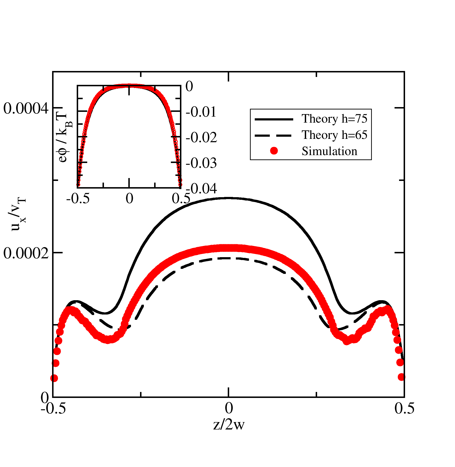
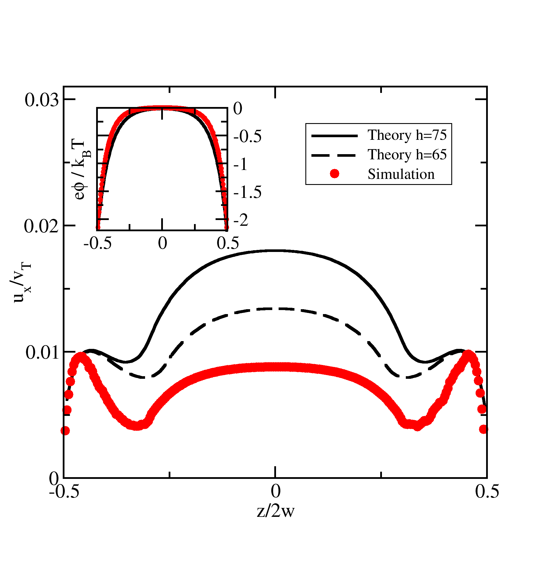
Figure 2: Neutral polymer coating. Velocity profiles for $\beta=0.1$ l.u. and two values of the surface charge density: $\Sigma/e=-3.9\times 10^{-5}$ (upper) and $\Sigma/e=-1.3\times 10^{-4}$ l.u. (lower panel). The simulation curve (circles) is obtained for $2w=250$ and $h=75$ l.u.. The two theoretical curves are obtained for $2w=250$ l.u. and $h=75$ (solid) and $65$ l.u. (dashed), respectively. Insets: electric potential profiles for each case.

We first consider the case of neutral polymers: the LBM results for the velocity and potential profiles are reported in fig. 2 and compared to the predictions of the analytical theory of section III. In the case of the smaller surface charge density $\Sigma/e=-3.9\times 10^{-5}$ l.u., the agreement is better than for $\Sigma/e=-1.3\times 10^{-4}$ l.u. . In fact, the linearization of the Poisson-Boltzmann eq. 19 introduces a systematic error which becomes larger when $|\Sigma|$ increases, as appreciated by comparing the two insets of fig. 2, where the analytical and numerical results for the potential are compared. The discrepancy displayed in the right inset has repercussions on the velocity profile, that is appreciably lower in the central region in the LBM case. The reason for the discrepancy can be traced back to the small gradient assumption used in the constitutive equation for the stress tensor, eq. 17, which ultimately leads to eq. 24. Near the walls the velocity gradients are quite large and the Stokes equation might be inadequate to capture the correct behavior. The difference between the analytic and the LBM velocity profiles decreases by setting $h=65$ l.u. in the analytical model and $h=75$ l.u. in the LBM. However, such a readjustement is insufficient to produce the same level of agreement in the case of larger surface charge, see fig. 2, right panel. Probably one can improve the matching by adjusting both the value of $\Sigma$ and $h$ in the analytical model, but we did not pursue further such a program because somehow arbitrary, although it could provide a simple and economical tool to scan the overall behavior of the system.

We consider, now, the case of charged coatings, where the electric potential depends altogether on the surface charge, the fixed charges associated with the fixed obstacles and the ionic charges in the EDL. For low values of the negative surface charge it is possible to observe a flow reversal in the presence of positive polymer charges. The density of mobile charges in the central region $|z|<h$ has the same sign as the surface charge when $\Sigma$ is lower than the value

$$\Sigma^{*} = \frac{ez_{s}n_{s}}{k_{D}}(\sinh(k_{D}h)e^{-k_{D}w}-\sinh(k_{D}w)e^{-k_{D}h})$$ (50)

$$\approx \begin{cases}-\frac{ez_{s}n_{s}}{2k_{D}}e^{k_{D}\delta}&\mbox{if }k_{D}\delta\gg 1\\ -ez_{s}n_{s}\delta&\mbox{if }k_{D}\delta\ll 1\,,\end{cases}$$

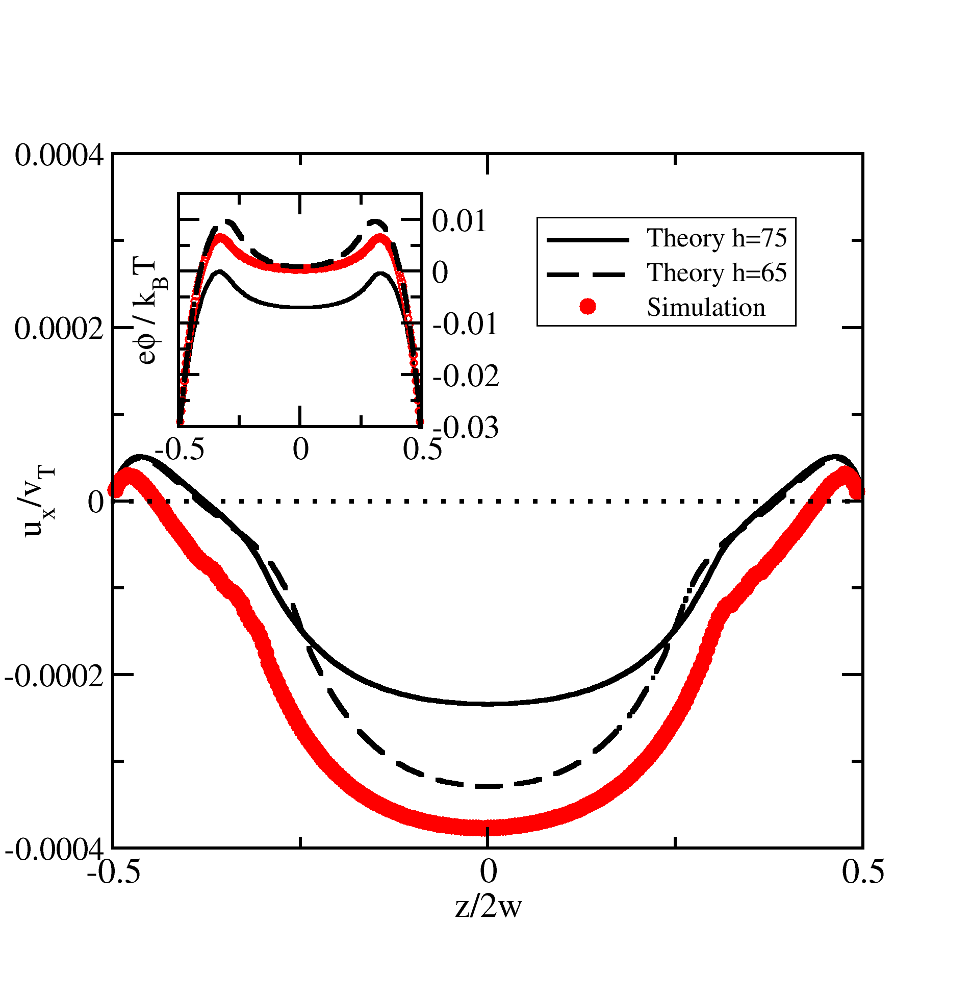
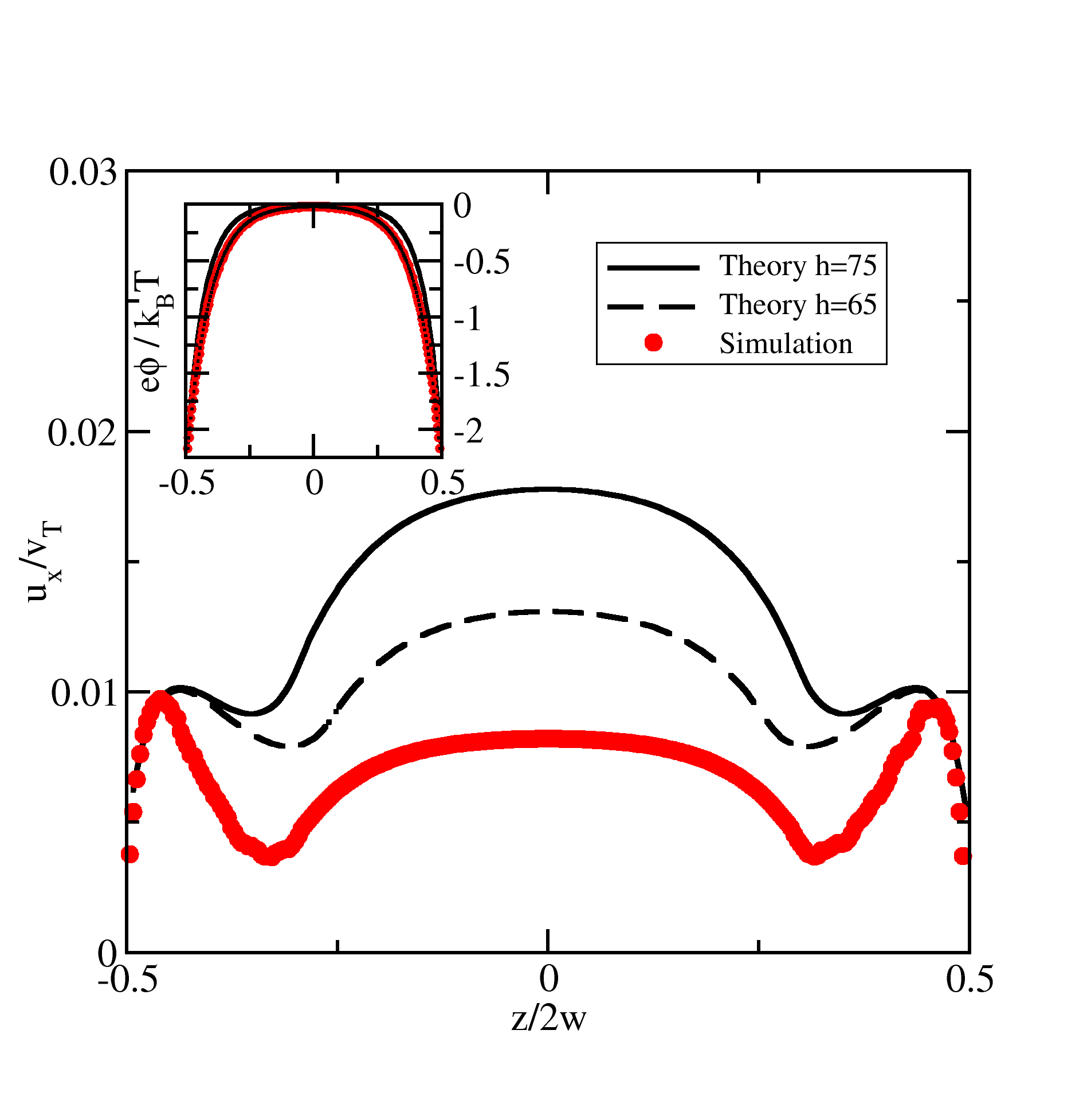
Figure 3: Charged polymer coating. Velocity profiles for $\beta=0.1$ l.u. and $\Sigma/e=-3.9\times 10^{-5}$ (upper) and $\Sigma/e=-1.3\times 10^{-4}$ l.u. (lower panel). Symbols as in fig. 2. Insets: electric potential profiles. Notice the flow reversal and the non-monotonic character of the potential for small surface charge density (left panel).

as one can see from eq. 21 and eq. 23. It is worth noting that the overall polymeric charge $z_{s}n_{s}\delta$ per unit surface does not need to be larger in absolute value than the negative surface charge sitting on the wall in order to induce flow reversal in the capillary, consistently with the earlier observation by Hickey et al. Hickey et al. (2011). It is important to remark that the regime studied in most of the existing literature Tessier and Slater (2006); Hickey et al. (2009); Cao et al. (2010, 2012) concerns small values of the Debye length, being typically $0.2\,nm$ . In this case, the EDL near the wall is not finely resolved and the comparison with the Smoluchowski theory is performed by taking the peak position of the velocity as shear plane, where the velocity assumes its maximum value $v_{sl}$ and its derivative vanishes. In our analytical model conducted at larger values of $\lambda_{D}$, instead, we can identify such a shear plane with the local maximum of the velocity, that appears in the region $h<|z|<w$, as a result of the competition between the drag force exerted by the polymers and the electro-osmotic force. Its location is at distance $\Delta\approx(k_{D}-\beta)\ln(\beta/k_{D})$ from each wall and the velocity decays towards the bulk from such a maximum in an exponential fashion. Only for small values of $\lambda_{D}$ the velocity profile displays two side peaks and no dome at the center. fig. 3 displays the results relative to a weakly charged polymer coating, while the remaining parameters are identical to those employed in fig. 2. Again, for small surface charge the agreement between the analytical result with the rescaled value of $h$ and the LB simulation is fairly good, but deteriorates at larger values of $\Sigma$ for the same reasons discussed above.

As displayed in the inset of fig. 3 left, the potential $\phi$ associated with a small negative surface charge, is non monotonic, reflecting the strong inhomogeneity of the ionic charge distribution: the regions adjacent the walls are richer of counterions, whereas further away the coions prevail. The direction of the mass flow occurs in the $x$ direction in the first region and in the opposite direction in the negatively populated region. Because of the relatively large value of the screening length of fig. 3 left one can see a large bulge in the center, while for $\lambda_{D}\ll\delta$ the flow inversion takes place only at the walls .

We obtained the solution of the Stokes eq. 24 by imposing the continuity of the derivative of the velocity at $z=\pm h$. However, the latter condition is not necessary in principle, and has been introduced after observing that the LBM velocity profiles do not display cusps. Without such a continuity requirement, the analytic velocity profiles obtained by setting the parameter $N=0$ in eq. 33 display lower values of the velocity in the central region, hence are closer to the LB result, but also displays a cusp which is not observed numerically.

The large $k_{D}w$ regime is of particular interest, because in the case of uncoated channels it displays plug-like velocity profiles: a very thin region near the walls of thickness $\lambda_{D}$ where the velocity raises from the zero value at the wall to the plateau value $u_{x}(0)$. The effect of the obstacles is dramatic: one observes only a single peak near each wall and the structure of the velocity profile depends weakly on $k_{D}$, the relevant length being, now, $\beta^{-1}$. If the polymer coating is sufficiently thick ($\beta\delta>1$), besides the peaks near the walls the velocity drops exponentially towards the center, with the characteristic length $\beta^{-1}$. The peaks result from the competition between the electroosmotic driving force, determining the growth of the velocity from the wall value (respecting the no-slip boundary conditions), and the antagonistic frictional force tending to suppress it.

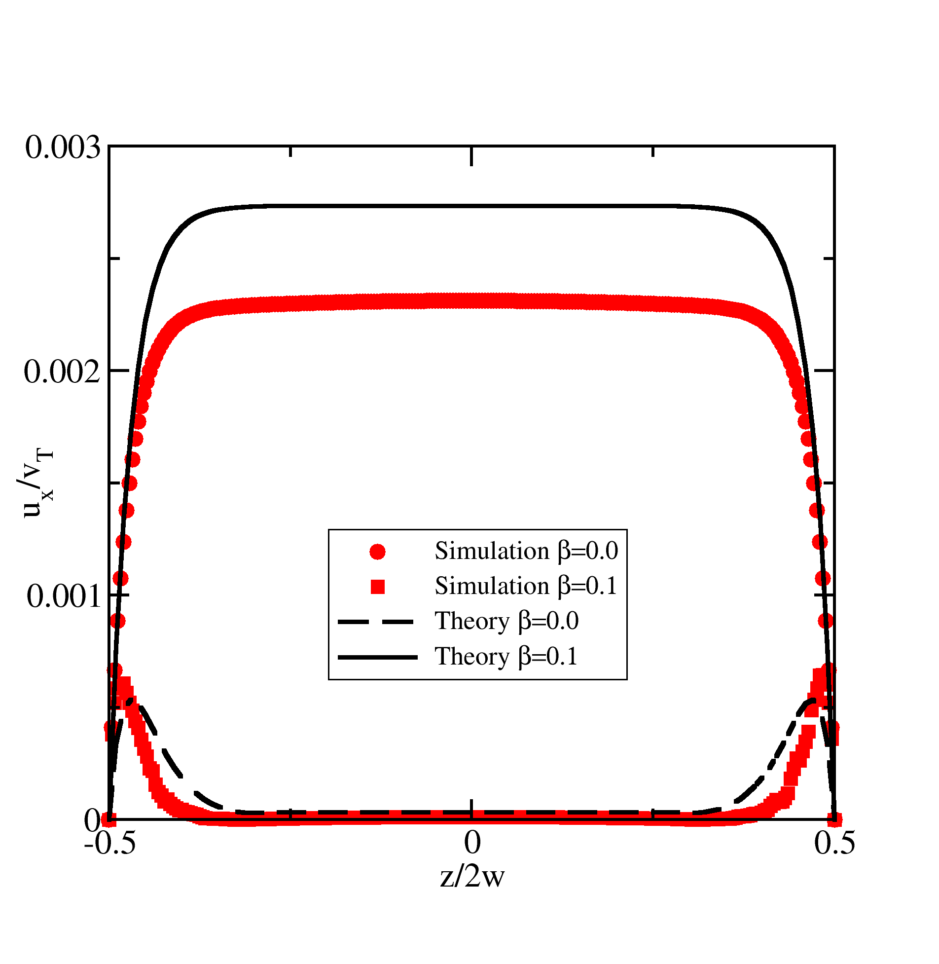
Figure 4: Theoretical (black) and simulation (red) velocity profiles, for a slit of width $w=250$, polymer thickness $\delta=50$ and neutral polymer. The curves correspond to $\beta=0$ (circles, solid) and $\beta=0.1$ l.u. (squares, dashed), and for $\Sigma/e=-1.3\times 10^{-4}$ l.u. and $\lambda_{D}=7.5$ l.u..

In this regime the coating appears to be very efficient in suppressing the mass flow, as shown in fig. 4. The continuity condition of the derivative of $u_{x}$ becomes irrelevant in the structure of the analytic solution since the cusp is hardly detectable and the difference between the solution with continuous derivative and discontinuous derivative is very small. We also remark that in the large $k_{D}$ regime, the flow reversal is characterized by the presence of two peaks near the walls, where most of the flow occurs, whereas in the small $k_{D}$ regime the majority of the flow occurs at the center of the slit.

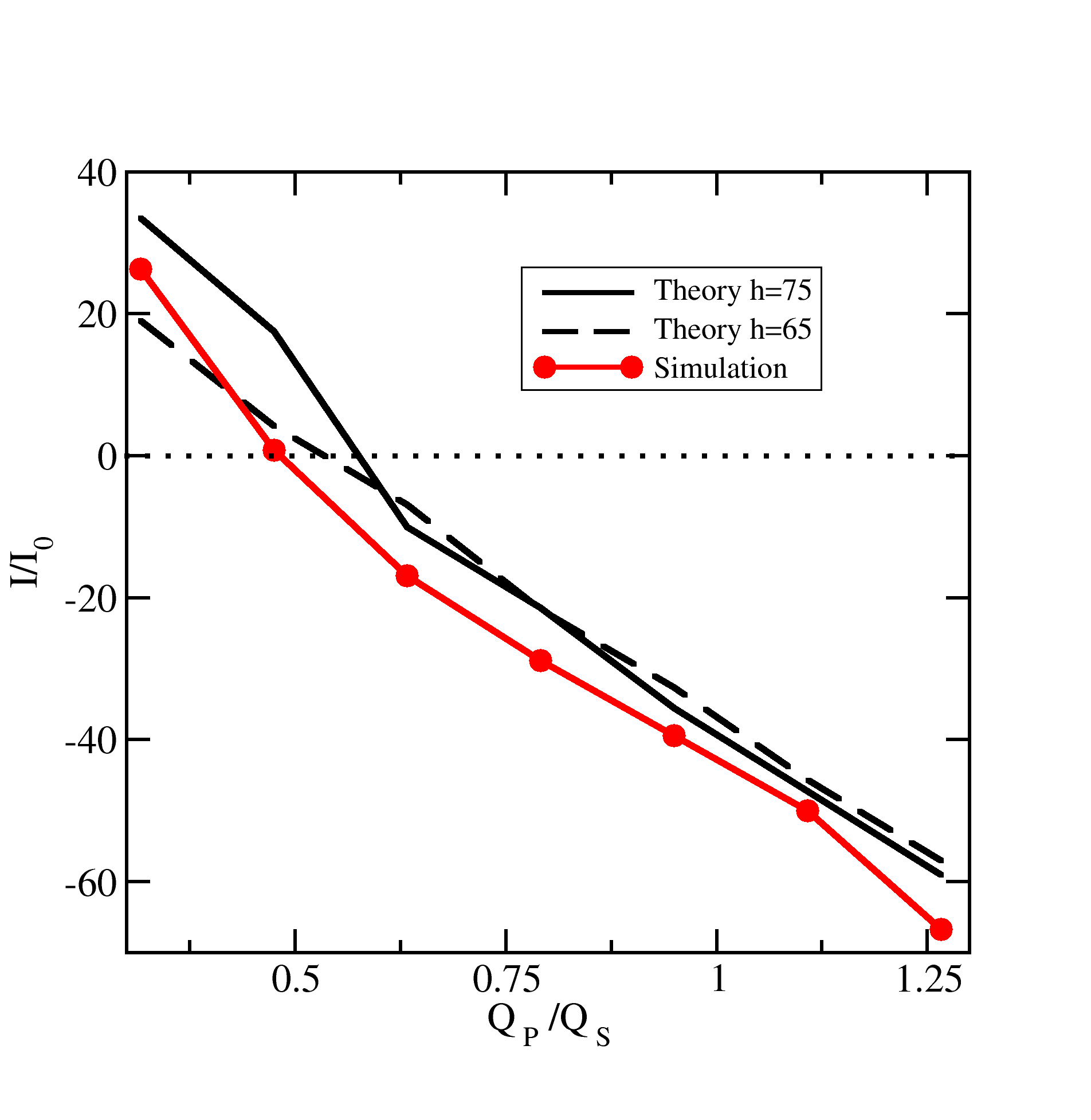
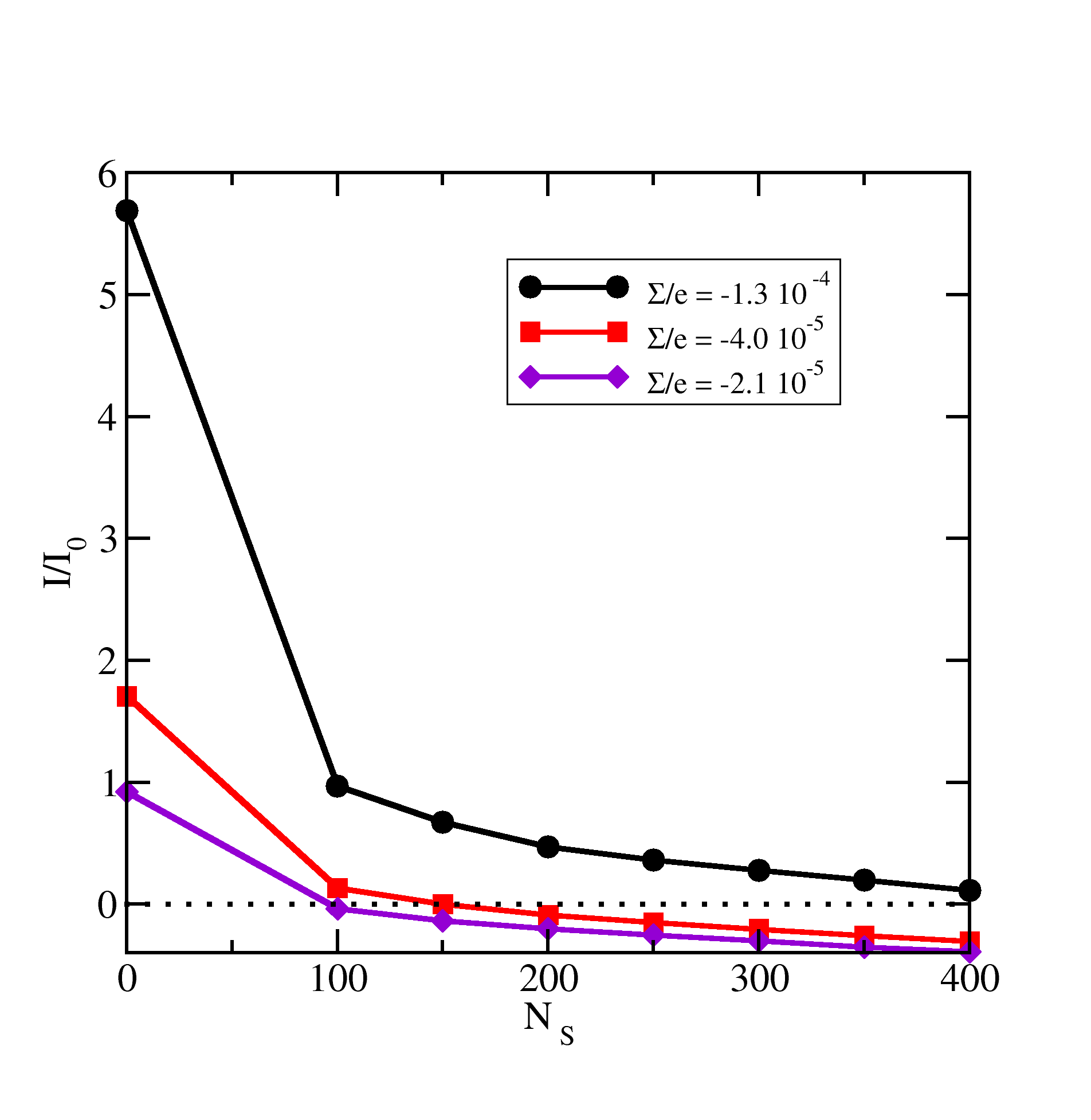
Figure 5: Scaled mass flow rate ($I_{0}=E_{x}\Sigma L_{x}L_{y}/\nu$) vs the ratio between the total surface and polymer charge $Q_{P}/Q_{S}$ (upper) and vs the number of charged obstacles for different values of the surface charge (lower panel). Data on the left panel correspond to simulation (red circles) and theoretical results (black) for $h=75$ (continuos line) and $65$ l.u. (dashed line), respectively. Data on the right panel are from simulations and for $\lambda_{D}=23$ l.u.. Notice the flow reversal for the two lowest values of the surface charge.

In fig. 5 we report the normalized mass flow rate as a function of the ratio between the total surface and total polymer charge. The theoretical and the simulation results are quite similar, and the difference between the theoretical curves $h=75$ and $h=65$ l.u. is not large. This figure shows that the analytic prediction, as far as channel averaged quantity is concerned, is quite accurate and can be used to give quantitative information about the global behavior. The right panel of fig. 5 displays the mass flow, $\Phi$, versus the number of charged obstacles, $N_{s}$, for different values of the surface charge. Clearly, $\Phi$ decreases with increasing values of $N_{s}$, due to the increased friction.

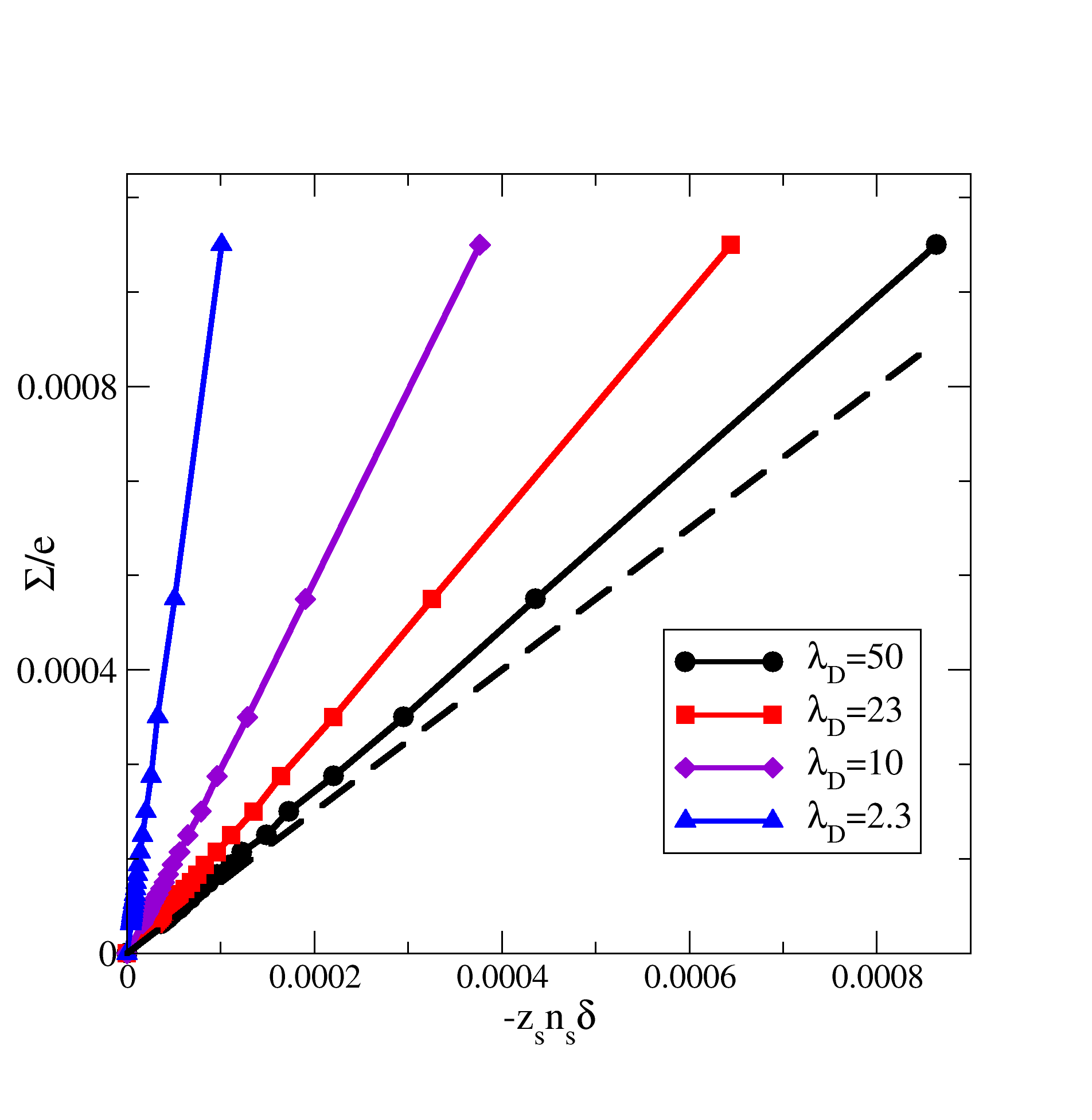
Figure 6: Phase diagram. The four lines correspond to $\lambda_{D}=50$ (circles), $23$ (squares), $10$ (diamonds) and $2.3$ l.u. (triangles up). The EOF is positive above each curve and negative below. The dashed line represents the line $-\Sigma/e=z_{s}n_{s}\delta$ obtained when the charge in the polymer layers equals the surface charge (local electroneutrality assumption), a limit valid in the weak screening regime ($\lambda_{D}>\delta$).

In fig. 6 we propose a phase diagram using the $\Sigma,(z_{s}n_{s}\delta)$ plane: above the curve the flow is in the positive direction, whereas below the curve the flows is reversed. The different curves correspond to different Debye lengths expressed in lattice units: $\lambda_{D}=2.3,10,23,50$ (blue, green, red, black). The dashed line represents the curve $-\Sigma^{*}=z_{s}n_{s}\delta$ the electroneutral line, that is, the line obtained by assuming that the charge in the polymer layer equals exactly the surface charge. Such a limit is attained in the weak screening regime ($\lambda_{D}>\delta$). For all Debye lengths considered, the demarcation curve between direct and reverse flow shows a linear shape. Notice the dependence of the slope of the line on the Debye length: the smaller $\lambda_{D}$ corresponds to steeper lines since the surface charge is screened faster and produces a smaller effect. The larger $\lambda_{D}$ the bigger the polymer charge density where the flow reversal occurs, since the effects of the surface extends over larger distances.

Finally we comment on the charge current, while the mass current is approximately linear with respect to $\Sigma$, the electric current is quadratic. Whereas the mass current displays inversion for small values of the surface charge and positive adsorbed polymers, the charge current does not. The reason is that the majority of the charge sits near the walls where the velocity is also large. The reversal of mass current is due to the fact that this is a flat average of $u_{x}(z)$, while the charge current is an average of $u_{x}(z)$ weighted by the local charge of carriers, and thus no inversion takes place.

VI Conclusions

In order to investigate the modulation of the electroosmotic flow in polymer coated capillaries we developed a phenomenological model and described the grafted polymers by a set of charged fixed obstacles exerting both a Coulomb force and a drag force on the fluid species. The electrolytic solution is represented by a ternary mixture and its behavior is studied numerically. By analyzing the resulting velocity profiles we found that the coating induces features that are not observed in standard EOF, such as non monotonicity, velocity inversion, suppression of the plug-like profile in the small $\lambda_{D}$ regime. This opens the possibility of designing functionalized capillary surfaces in order to improve the resolution in capillary electrophoresis. A remarkable feature of the model is that it lends itself to an analytical treatment in the case of moderate surface charges, so that the rather complex behavior in terms of a reduced set of parameters can be predicted. We have obtained the explicit analytical solution of the linearized model and shown that it agrees at semi-quantitative level with the numerical solutions.

Our approach replaces the complexity of the polymer layer by an assembly of scatterers and thus neglects many important aspects such as the deformability of the polymers under the flow, their connectivity, or the possibility of forming mushroom or brush structures as discussed by Harden et al. Harden et al. (2001) . Experimentally it would be important to establish a closer connection between our parameters $\delta$ and $\beta$ to the degree of polymerization $N$ (related the polymer thickness in the brush regime) and to the number density of grafted polymers onto a flat surface, respectively, instead of fixing them by a fitting procedure. Another intriguing aspect that can be investigated by our methods is the role played by the charge distribution within the polymer layer on the resulting EOF. As an example, Danger et al. Danger et al. (2007) used polyelectrolytes of different charge densities to control the EOF, obtained by depositing a first cationic polyelectrolyte layer followed by depositing a second polyelectrolyte layer based on anionic copolymer.

Before concluding, we remark that the differences between the planar and the cylindrical geometry are quantititatve rather than qualitative, so that it is possible to extend the present approach to include such a geometry, with an analytic treatment slightly more involved and less transparent.

VII Acknowledgments

This work was supported by the Italian Ministry of University and Research through the “Futuro in Ricerca” project RBFR12OO1G - NEMATIC. The authors wish to thank Marina Cretich, Marcella Chiari and Laura Sola for insightful discussions.

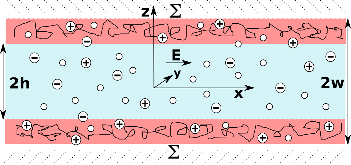
Figure 1: Sketch of the pore system. The near-wall regions represent the polymer coating, the small circles represent the solvent particles, the large circles represent counter and co-ions.

References

- Bruus (2008) H. Bruus, Theoretical microfluidics, Oxford University Press, 2008, vol. 18.
- Berthier and Silberzan (2010) J. Berthier and P. Silberzan, Microfluidics for biotechnology, Artech House, 2010.
- Kirby (2010) B. Kirby, Micro-and nanoscale fluid mechanics: transport in microfluidic devices, Cambridge University Press, 2010.
- Nguyen and Wereley (2002) N.-T. Nguyen and S. T. Wereley, Fundamentals and applications of microfluidics, Artech House, 2002.
- Masliyah and Bhattacharjee (2006) J. H. Masliyah and S. Bhattacharjee, Electrokinetic and colloid transport phenomena, John Wiley & Sons, 2006.
- Tabeling and Bocquet (2014) P. Tabeling and L. Bocquet, Lab on a Chip, 2014.
- Rotenberg and Pagonabarraga (2013) B. Rotenberg and I. Pagonabarraga, Molecular Physics, 2013, 111, 827–842.
- Kontturi et al. (2008) K. Kontturi, L. Murtomäki and J. A. Manzanares, Ionic transport processes: in electrochemistry and membrane science, OUP Oxford, 2008.
- Hickey et al. (2011) O. A. Hickey, C. Holm, J. L. Harden and G. W. Slater, Macromolecules, 2011, 44, 9455–9463.
- Hickey et al. (2012) O. A. Hickey, J. L. Harden and G. W. Slater, Microfluidics and nanofluidics, 2012, 13, 91–97.
- Monteferrante et al. (2014) M. Monteferrante, S. Melchionna, U. M. B. Marconi, M. Cretich, M. Chiari and L. Sola, Microfluidics and Nanofluidics, 2014, 1–8.
- Danger et al. (2007) G. Danger, M. Ramonda and H. Cottet, Electrophoresis, 2007, 28, 925–931.
- Doherty et al. (2002) E. A. Doherty, K. D. Berglund, B. A. Buchholz, I. V. Kourkine, T. M. Przybycien, R. D. Tilton and A. E. Barron, Electrophoresis, 2002, 23, 2766–2776.
- Znaleziona et al. (2008) J. Znaleziona, J. Petr, R. Knob, V. Maier and J. Ševčík, Chromatographia, 2008, 67, 5–12.
- Horvath and Dolník (2001) J. Horvath and V. Dolník, Electrophoresis, 2001, 22, 644–655.
- Chiari et al. (2000) M. Chiari, M. Cretich, F. Damin, L. Ceriotti and R. Consonni, Electrophoresis, 2000, 21, 909–916.
- Shendruk et al. (2012) T. Shendruk, O. Hickey, G. Slater and J. Harden, Current Opinion in Colloid & Interface Science, 2012, 17, 74–82.
- Harden et al. (2001) J. Harden, D. Long and A. Ajdari, Langmuir, 2001, 17, 705–715.
- Qiao and He (2007) R. Qiao and P. He, Langmuir, 2007, 23, 5810–5816.
- Cao et al. (2010) Q. Cao, C. Zuo, L. Li, Y. Ma and N. Li, Microfluidics and nanofluidics, 2010, 9, 1051–1062.
- Cao et al. (2012) Q. Cao, C. Zuo, L. Li and Y. Zhang, Microfluidics and nanofluidics, 2012, 12, 649–655.
- Tessier and Slater (2006) F. Tessier and G. W. Slater, Macromolecules, 2006, 39, 1250–1260.
- Hickey et al. (2009) O. A. Hickey, J. L. Harden and G. W. Slater, Physical review letters, 2009, 102, 108304.
- Benzi et al. (1992) R. Benzi, S. Succi and M. Vergassola, Physics Reports, 1992, 222, 145–197.
- Karniadakis et al. (2006) G. Karniadakis, A. Beskok and N. R. Aluru, Microflows and nanoflows: fundamentals and simulation, Springer, 2006, vol. 29.
- Looker (2006) J. R. Looker, The electrokinetics of porous colloidal particles, PhD Thesis. University of Melbourne, Department of Mathematics and Statistics, 2006.
- Melchionna and Marini Bettolo Marconi (2011) S. Melchionna and U. Marini Bettolo Marconi, EPL (EuroPhysics Letters), 2011, 95, 44002.
- Bhatnagar et al. (1954) P. L. Bhatnagar, E. P. Gross and M. Krook, Physical review, 1954, 94, 511.
- Marini Bettolo Marconi and Melchionna (2012) U. Marini Bettolo Marconi and S. Melchionna, Langmuir, 2012, 28, 13727–13740.
- Marini Bettolo Marconi and Melchionna (2011) U. Marini Bettolo Marconi and S. Melchionna, The Journal of Chemical Physics, 2011, 134, 064118–064118.
- Marini Bettolo Marconi and Melchionna (2011) U. Marini Bettolo Marconi and S. Melchionna, The Journal of Chemical Physics, 2011, 135, 044104.
- Cao et al. (2011) Q. Cao, C. Zuo, L. Li, Y. Yang and N. Li, Microfluidics and nanofluidics, 2011, 10, 977–990.
- Monteferrante et al. (2014) M. Monteferrante, S. Melchionna and U. M. B. Marconi, The Journal of chemical physics, 2014, 141, 014102.