Lorentz Dispersion Law from classical Hydrogen electron orbits
in AC electric field via geometric algebra

Abstract

We studied the orbit of an electron revolving around an infinitely massive nucleus of a large classical Hydrogen atom subject to an AC electric field oscillating perpendicular to the electron’s circular orbit. Using perturbation theory in geometric algebra, we show that the equation of motion of the electron perpendicular to the unperturbed orbital plane satisfies a forced simple harmonic oscillator equation found in Lorentz dispersion law in Optics. We show that even though we did not introduce a damping term, the initial orbital position and velocity of the electron results to a solution whose absorbed energies are finite at the dominant resonant frequency $\omega=\omega_{0}$; the electron slowly increases its amplitude of oscillation until it becomes ionized. We computed the average power absorbed by the electron both at the perturbing frequency and at the electron’s orbital frequency. We graphed the trace of the angular momentum vector at different frequencies. We showed that at different perturbing frequencies, the angular momentum vector traces epicyclical patterns.

I Introduction

In standard optics texts, the position $x$ of an electron of charge $q$ and mass $m$ under the time-varying electric field $E=\mathcal{E}e^{i\omega t}$ of light is given byJackson (1975); Zangwill (2013); Klein and Furtak (1986)

$$\ddot{x}+\Gamma\dot{x}+\omega_{0}^{2}x=\frac{q}{2m}E,$$ (1)

where $\Gamma$ is the damping coefficient, $\omega_{0}$ is the natural frequency of oscillation of the electron. The complex solution $\tilde{x}$ to this equation is shown by Akhmanov and Nikitin Akhmanov and Nikitin (1997) to be

$$\tilde{x}=\frac{q}{m}\frac{1}{\omega^{2}_{0}-\omega^{2}+i\omega\Gamma}\mathcal{E},$$ (2)

so that the power absorbed by the atom is

$$\langle P\rangle=\langle qE\dot{x}\rangle=\frac{q^{2}}{2m}\frac{\omega^{2}\Gamma}{(\omega^{2}_{0}-\omega^{2})^{2}+\omega^{2}\Gamma^{2}}|\mathcal{E}|^{2},$$ (3)

which in complex space becomes

$$P=\frac{e}{4}i\omega\left(\mathcal{E}^{*}\tilde{x}+\mathcal{E}\tilde{x}e^{2i\omega t}\right).$$ (4)

Notice that the damping term $\Gamma$ makes the power absorbed finite at the resonant frequency $\omega=\omega_{0}$.

At present it is still not clear why an atom can be described as a simple harmonic oscillator subject to sinusoidal electric field of light, e.g. what is responsible for the restoring force constant $k=m\omega^{2}_{0}$ and what is the cause of damping force $\Gamma\dot{x}$?

In this paper we wish to show that a forced harmonic oscillator equation can arise for a large Hydrogen atom with a circular orbital of frequency $\omega_{0}$ subject to a linearly polarized light of frequency $\omega$ whose corresponding wavelength $2\pi c/\omega$ is much larger than the electron’s orbital radius $r_{0}$, e.g. microwave frequencies, so that the phase of light is approximately the same at any point in the orbital path within a certain time period. That is, if the electron is initially in circular orbit in the $xy$-plane, the position $s$ of the electron along the $z$-axis is given by

$$\ddot{s}+\bm{\omega_{o}^{2}}s=-\frac{qE}{m}\cos\left(\omega t\right),$$ (5)

as similarly given in Born and Wolf M.Born and Wolf (1964). Even though this equation does not have a damping term, we shall show that the energy absorbed at the resonant frequency $\omega=\omega_{0}$ remains finite, provided we take into account the position $\mathbf{r}$ of the electron in 3D and use the vector form of the electrical energy dissipation expression Jackson (1975):

$$P=q\mathbf{E}\cdot\mathbf{\dot{r}}.$$ (6)

We shall show that $\langle P\rangle$ is finite at the resonant frequency $\omega=\omega_{0}$ even though there is no damping.

In 1974, Bayfield and Koch experimentally studied the ionization of hydrogen atoms under microwave frequencies Bayfield and Koch (1974). Since then, many tried to study the interaction of microwave radiation with classical hydrogen atom within the context of Rydberg atoms.Haken and Wolf (2000) Some authors studied the interaction with circularly polarized light Cole and Zou (2004); Brunello et al. (1996); Farelly and Uzer (1995); Farelly and Griffiths (1992); Gajda et al. (1994), while others such as Leopold Leopold and Percival (1978), Grosfeld and Friedland Grosfeld and Friedland (2002) and Neishtadt Neishtadt and Vasiliev (2005) focused on the linearly polarized case.

For Leopold, his Hamiltonian is of the form:

$$H(\vec{r},\vec{p})=\frac{1}{2}p^{2}-r^{-1}+zF_{max}\cos\omega t,$$ (7)

and the equations are solved using Monte-Carlo techniques. For Grosfeld and Friedland, their Hamiltonian is of the form:

$$H=\frac{1}{2}p^{2}-r^{-1}+Z\mu\cos\Psi,$$ (8)

where the frequency $\omega(t)=d\Psi/dt$ and the authors used action angle variables. This Hamiltonian is the same one used by Neishtadt and Vasiliev, except that the latter authors used Delaunay elements.

In our work, we shall not use the Hamiltonian approach. Instead, we shall use the force equation

$$\ddot{\mathbf{r}}=-\frac{kq^{2}}{m}\frac{\mathbf{r}}{|\mathbf{r}|^{3}}-\lambda\mathbf{e}_{3}\frac{q}{m}E_{0}\cos(\omega t+\varphi),$$ (9)

and use linear perturbation theory to simplify the equation to a simple harmonic oscillator equation in (5) for a motion perpendicular to the initial circular orbital plane of the electron. This method is simpler than those of the previous authors because the solution to the simple harmonic oscillator equation is well-known. Just as in the optical dispersion theory, we computed for the average power absorption by the atom and showed that it only depends on the $z$-coordinate as in the standard theory.

$$\langle P\rangle_{\tau}=\frac{1}{\tau}\int_{0}^{\tau}P\,dt.$$ (10)

We shall show that the orbit of the electrons at integral frequency ratios are similar to De Broglie waves, except that the oscillation is perpendicular to the electron’s orbital plane.

We shall divide the paper into six sections. Section 1 is Introduction. In Section 2, we shall discuss the Geometric Algebra formalism applied to planar rotations. In Section 3, we shall describe the unperturbed circular orbit of the electron around the nucleus. After this, we shall introduce an oscillating electric field perturbation and derive the equations of motion of the electron’s oscillation perpendicular to its orbital plane, using the geometric algebra framework in our previous paper on Copernican epicyclical orbitsSugon Jr. et al. (2008). In Section 4, we shall compute the electron’s orbital angular momentum and determine its limiting form at the resonant frequency. In Section 5, we shall compute the electrical power dissipation of the electron and plot the results for different values of the ratio between the orbital and light frequencies. We shall show that the average power, either over the perturbing or orbital period, is approximately similar to the standard absorption resonance curve with finite peak. Finally, we graph the angular momentum of the electron at different frequency ratios and show that the angular momentum vector traces epicyclical patterns.

II Geometric Algebra

II.1 Scalars, Vectors, Bivectors, and Trivectors

In Clifford (Geometric) Algebra $\mathcal{C}l_{3,0}$, also known as the Pauli Algebra, the product of the three unit vectors $\mathbf{e}_{1}$,$\mathbf{e}_{2}$, and $\mathbf{e}_{3}$ satisfies the orthonormality relation Vold (1993); Hestenes (2003); Sugon Jr. and McNamara (2004)

$$\mathbf{e}_{j}\mathbf{e}_{k}+\mathbf{e}_{k}\mathbf{e}_{j}=2\delta_{jk},$$ (11)

where $\delta_{jk}$ is the Kronecker delta function. In other words, the square of the length of the vectors is equal to one and the product of two perpendicular vectors anticommute.

Let $\mathbf{a}$ and $\mathbf{b}$ be two vectors spanned by $\mathbf{e}_{1}$, $\mathbf{e}_{2}$, and $\mathbf{e}_{3}$. We can show that their product satisfies the Pauli identityBaylis (1996); Lounesto (2001)

$$\mathbf{a}\mathbf{b}=\mathbf{a}\cdot\mathbf{b}+i(\mathbf{a}\times\mathbf{b}),$$ (12)

where $i=\mathbf{e}_{1}\mathbf{e}_{2}\mathbf{e}_{3}$ is the unit trivector which behaves like an imaginary scalar that transforms vectors to bivectors. The Pauli identity states that the geometric product of two vectors is equal to the sum of their scalar dot product and their imaginary cross product.

II.2 Exponential Function and Rotations

Let $i\mathbf{e}_{3}\theta$ be the product of a bivector $i\mathbf{e}_{3}=\mathbf{e}_{1}\mathbf{e}_{2}$ with the scalar $\theta$. Since the square of $i\mathbf{e}_{3}\theta$ is negative, then the exponential of $i\mathbf{e}_{3}\theta$ is given by Euler’s theorem

$$e^{i\mathbf{e}_{3}\theta}=\cos\theta+i\mathbf{e}_{3}\sin\theta.$$ (13)

From this we can see that

$$\cos\theta =\frac{1}{2}(e^{i\mathbf{e}_{3}\theta}+e^{-i\mathbf{e}_{3}\theta}),$$ (14a)

$$\sin\theta =\frac{1}{2i\mathbf{e}_{3}}(e^{i\mathbf{e}_{3}\theta}-e^{-i\mathbf{e}_{3}\theta}),$$ (14b)

which are the known exponential definitions of cosine and sine functions.

\begin{overpic}[width=151.76633pt,tics=5,page=1]{rydberg_version2_graphics} \put(97.0,68.0){$\mathbf{e}_{1}e^{i\mathbf{e}_{3}\theta}$} \put(15.0,94.0){$\mathbf{e}_{2}e^{i\mathbf{e}_{3}\theta}$} \put(47.0,101.0){$\mathbf{e}_{2}$} \put(100.5,45.0){$\mathbf{e}_{1}$} \put(65.0,48.0){$\theta$} \put(45.0,62.0){$\theta$} \end{overpic}

Figure 1: Rotation of $\mathbf{e}_{1}$ and $\mathbf{e}_{2}$ about $\mathbf{e}_{3}$ counterclockwise by an angle $\theta$

Multiplying Eq. (13) by $\mathbf{e}_{1}$, $\mathbf{e}_{2}$, and $\mathbf{e}_{3}$, we obtain

$$\mathbf{e}_{1}e^{i\mathbf{e}_{3}\theta} =\mathbf{e}_{1}\cos\theta+\mathbf{e}_{2}\sin\theta=e^{-i\mathbf{e}_{3}\theta}\mathbf{e}_{1},$$ (15a)

$$\mathbf{e}_{2}e^{i\mathbf{e}_{3}\theta} =\mathbf{e}_{2}\cos\theta-\mathbf{e}_{1}\sin\theta=e^{-i\mathbf{e}_{3}\theta}\mathbf{e}_{2},$$ (15b)

$$\mathbf{e}_{3}e^{i\mathbf{e}_{3}\theta} =\mathbf{e}_{3}\cos\theta+\mathbf{e}_{3}i\mathbf{e}_{3}\sin\theta=e^{i\mathbf{e}_{3}\theta}\mathbf{e}_{3}.$$ (15c)

Notice that $\mathbf{e}_{1}e^{i\mathbf{e}_{3}\theta}$ is a rotation of $\mathbf{e}_{1}$ counterclockwise about $\mathbf{e}_{3}$ by an angle $\theta$, while $\mathbf{e}_{2}e^{i\mathbf{e}_{3}\theta}$ is a rotation of $\mathbf{e}_{2}$ counterclockwise about the same direction and the same angle. Notice, too, that the argument of the exponential changes sign when $\mathbf{e}_{1}$ or $\mathbf{e}_{2}$ trades places with the exponential, while $\mathbf{e}_{3}$ commutes with the exponential.

A vector $\mathbf{a}$ in 2D can be expressed in both rectangular and polar forms:

$$\mathbf{a}=a_{x}\mathbf{e}_{1}+a_{y}\mathbf{e}_{2}=a\mathbf{e}_{1}e^{i\mathbf{e}_{3}\theta}.$$ (16)

Expanding the exponential using Eq. (15a) and separating the $\mathbf{e}_{1}$ and $\mathbf{e}_{2}$ components, we arrive at the standard transformation equations for polar to rectangular coordinates:

$$x =a\cos\theta,$$ (17a)

$$y =a\sin\theta.$$ (17b)

We may also factor out $\mathbf{e}_{1}$ in Eq. (16) either to the left or to the right to get

$$\mathbf{a} =\mathbf{e}_{1}\hat{a}=\mathbf{e}_{1}(x+i\mathbf{e}_{3}y)=\mathbf{e}_{1}ae^{i\mathbf{e}_{3}\theta},$$ (18a)

$$\mathbf{a} =\hat{a}^{*}\mathbf{e}_{1}=(x-i\mathbf{e}_{3}y)\mathbf{e}_{1}=ae^{-i\mathbf{e}_{3}\theta}\mathbf{e}_{1}.$$ (18b)

Factoring out $\mathbf{e}_{1}$ yields the definition of the complex number $\hat{a}$ and that of its complex conjugate $\hat{a}^{*}$:

$$\hat{a} =a_{x}+i\mathbf{e}_{3}a_{y}=ae^{i\mathbf{e}_{3}\theta},$$ (19a)

$$\hat{a}^{*} =a_{x}-i\mathbf{e}_{3}a_{y}=ae^{-i\mathbf{e}_{3}\theta}.$$ (19b)

In general, we have the following relations:

$$\mathbf{e}_{1}\hat{a} =\hat{a}^{*}\mathbf{e}_{1},$$ (20a)

$$\mathbf{e}_{2}\hat{a} =\hat{a}^{*}\mathbf{e}_{2},$$ (20b)

$$\mathbf{e}_{3}\hat{a} =\hat{a}\mathbf{e}_{3}.$$ (20c)

That is, $\mathbf{e}_{1}$ and $\mathbf{e}_{2}$ both changes the complex number $\hat{a}$ to its conjugate $\hat{a}^{*}$ after commutation, while $\mathbf{e}_{3}$ simply commutes with $\hat{a}$ Jancewicz (1989); Sugon Jr. and McNamara (2004); Vold (1993); Hestenes (2003).

III Light-Atom Interaction

III.1 Unperturbed Electron Orbit

Classically, the position $\mathbf{r}$ of an electron of mass $m$ and charge $-q$ as it revolves around a massive proton of charge $q$ is given by Coulomb’s law:

$$\ddot{\mathbf{r}}=-\frac{kq^{2}}{m}\frac{\mathbf{r}}{|\mathbf{r}|^{3}},$$ (21)

where $k$ is the electrostatic force constant. We claim that a solution to Eq. (21) is given by

$$\mathbf{r}=\mathbf{r}_{0}=\mathbf{e}_{1}\hat{r}_{0}\hat{\psi}_{0},$$ (22)

where

$$\hat{r}_{0} =r_{0}e^{i\mathbf{e}_{3}\varphi_{0}}$$ (23a)

$$\hat{\psi}_{0} =e^{i\mathbf{e}_{3}\omega_{0}t}$$ (23b)

are the complex amplitude and the rotation operator, respectively. Substituting these back to Eq. (22), we get

$$\mathbf{r}_{0}=\mathbf{e}_{1}r_{0}e^{i\mathbf{e}_{3}(\omega_{0}t+\varphi_{0})},$$ (24)

which yields

$$\mathbf{r}_{0}=\mathbf{e}_{1}r_{0}\cos(\omega_{0}t+\varphi_{0})+\mathbf{e}_{2}r_{0}\sin(\omega_{0}t+\varphi_{0}),$$ (25)

after expanding the exponential and distributing $\mathbf{e}_{1}$. Equation (22) states that the electron moving around the proton in circular orbit of radius $r_{0}$ with angular velocity $\omega_{0}$ and rotational phase angle $\varphi_{0}$.

\begin{overpic}[width=130.08731pt,tics=5,page=2]{rydberg_version2_graphics} \put(69.0,97.0){$r_{0}\mathbf{e}_{1}e^{i\mathbf{e}_{3}(\varphi+\omega t)}$} \put(97.0,68.0){$r_{0}\mathbf{e}_{1}e^{i\mathbf{e}_{3}\varphi}$} \put(100.5,45.0){$r_{0}\mathbf{e}_{1}$} \put(65.0,50.0){$\varphi$} \put(60.0,59.0){$\omega t$} \end{overpic}

Figure 2: Uniform circular motion of an electron with a distance $r_{0}$ from the nucleus. The orbital angular frequency is $\omega$ and the phase angle is $\varphi$.

To verify that Eq. (22) is indeed a solution to the Coulomb’s law in Eq. (21), we first compute the first and second time derivatives of Eq. (22):

$$\dot{\mathbf{r}} =\mathbf{e}_{1}\hat{r}_{0}i\mathbf{e}_{3}\omega_{o}\hat{\psi}_{0},$$ (26a)

$$\ddot{\mathbf{r}} =-\mathbf{e}_{1}\hat{r}_{0}\omega_{0}^{2}\hat{\psi}_{0}.$$ (26b)

Now, substituting Eqs. (22) and (26b) to the Coulomb’s law in Eq. (21), we obtain

$$\omega_{o}^{2}=\frac{kq^{2}}{mr_{0}^{3}},$$ (27)

after cancelling out $\mathbf{e}_{1}\hat{r}_{0}\hat{\psi}_{0}$. Equation (27) is the familiar circular orbit condition.

III.2 Perturbation by an Oscillating Field

Suppose that the electron is subject not only to the Coulomb force $-q\mathbf{E}_{c}$ due to the proton, but also to the force $-q\mathbf{E}_{p}$ due to an oscillating perturbing field. The equation of motion of the electron then becomes

$$m\ddot{\mathbf{r}}=-q\mathbf{E}_{c}-\lambda q\mathbf{E}_{p},$$ (28)

where $\lambda$ is a perturbation parameter that shall later be set equal to unity. More specifically, we write

$$\ddot{\mathbf{r}}=-\frac{kq^{2}}{m}\frac{\mathbf{r}}{|\mathbf{r}|^{3}}-\lambda\mathbf{e}_{3}\frac{q}{m}E_{0}\cos(\omega t+\varphi),$$ (29)

where $E_{0}$, $\omega$, and $\varphi$ are the amplitude, angular frequency, and phase of the perturbing electric field. Our aim is to determine the position $\mathbf{r}$ of the electron that satisfies Eq. (29).

\begin{overpic}[width=151.76633pt,tics=5,page=3]{rydberg_version2_graphics} \put(31.0,17.0){$+|q|$} \put(77.0,2.0){$-|q|$} \put(47.0,10.0){$\mathbf{F}_{c}$} \put(71.0,43.0){$\mathbf{F}_{p}$} \put(100.0,20.0){$\mathbf{v}_{0}$} \put(55.0,17.0){$r_{0}$} \end{overpic}

Figure 3: The Coulomb force $\mathbf{F}_{c}$ and the perturbing force $\mathbf{F}_{p}$ on an electron moving with velocity $\mathbf{v}_{0}$ and radius $r_{0}$

To find the solution to the perturbed orbit equation in Eq. (29), we assume that the solution is a sum of the electron’s unperturbed circular orbit in Eq. (22) and a slight perturbation $\hat{s}$ perpendicular to this orbit. So we write

$$\mathbf{r}=\mathbf{r}_{0}+\lambda\mathbf{r}_{1}=\mathbf{e}_{1}\hat{r}_{0}\hat{\psi}_{0}+\lambda\mathbf{e}_{3}\hat{s}.$$ (30)

The first and second time derivatives of $\mathbf{r}$ are

$$\dot{\mathbf{r}} =\dot{\mathbf{r}}_{0}+\lambda\dot{\mathbf{r}}_{1}=\mathbf{e}_{1}\hat{r}_{0}i\mathbf{e}_{3}\omega_{0}\hat{\psi}_{0}+\lambda\mathbf{e}_{3}\dot{\hat{s}},$$ (31a)

$$\mathbf{\ddot{r}} =\mathbf{\ddot{r}}_{0}+\lambda\mathbf{\ddot{r}}_{1}=-\mathbf{e}_{1}\hat{r}_{0}\omega_{o}^{2}\hat{\psi}_{0}+\lambda\mathbf{e}_{3}\ddot{\hat{s}}.$$ (31b)

Equation (31b) shall take care of the left side of Eq. (29).

To expand the right-hand side, we need first to take the square of the position vector $\mathbf{r}$ in Eq. (30) and retain only the terms up to first order in $\lambda$:

$$\mathbf{r}^{2}=\mathbf{r}_{0}^{2}+2\lambda(\mathbf{r}_{0}\cdot\mathbf{r}_{1}).$$ (32)

Since $\mathbf{r}_{0}$ lies on the unperturbed orbital plane of the electron $xy$ plane and $\mathbf{r}_{1}=\mathbf{e}_{3}$ is perpendicular to this plane, then $\mathbf{r}_{0}\cdot\mathbf{r}_{1}=0$, so that Eq. (32) reduces to

$$\mathbf{r}^{2}=\mathbf{r}_{0}^{2} =\mathbf{e}_{1}\hat{r}_{0}\hat{\psi}_{0}\,\mathbf{e}_{1}\hat{r}_{0}\hat{\psi}_{0}=\mathbf{e}_{1}\mathbf{e}_{1}\hat{r}_{0}^{*}\hat{\psi}_{0}^{*}\hat{r}_{0}\hat{\psi}_{0}$$

$$=\hat{r}_{0}^{*}\hat{r}_{0}=r_{0}^{2},$$ (33)

where we used the definitions of $\hat{r}_{0}$ and $\hat{\psi}_{0}$ in Eqs. (23a) and (23b). Thus, $|\mathbf{r}|=r_{0}$, so that

$$\frac{\mathbf{r}}{|\mathbf{r}|^{3}}=\frac{1}{r_{0}^{3}}\mathbf{e}_{1}\hat{r}_{0}\hat{\psi}_{0}.$$ (34)

Equation (34) shall take care of the Coulomb term on the right side of Eq. (29).

Now, substituting Eqs. (31b) and (34) back to equation of motion in Eq. (29), we obtain

$$-\mathbf{e}_{1}\hat{r}_{0}\omega_{o}^{2}\hat{\psi}_{0}+\lambda\mathbf{e}_{3}\ddot{s} =-\omega_{0}^{2}(\mathbf{e}_{1}\hat{r}_{0}\hat{\psi}_{0}+\lambda\mathbf{e}_{3}\hat{s})$$

$$\quad\ -\lambda\mathbf{e}_{3}\frac{q}{m}E_{0}\cos(\omega t+\varphi),$$ (35)

where we used the circular orbit condition in Eq. (27). The term zeroth order in $\lambda$ cancels out, so we are left with the term first order in $\lambda$. Hence,

$$\ddot{\hat{s}}+\omega_{0}^{2}\hat{s}=-\frac{q}{m}E_{0}\cos(\omega t+\varphi),$$ (36)

after rearranging the terms. Notice that Eq. (36) is a simple harmonic oscillator equation with sinusoidal forcing, which is the standard model for classical light-atom interaction.

III.3 Solving the Forced Harmonic Oscillator Equation

Let $\hat{s}_{h}$ and $\hat{s}_{p}$ be the homogeneous and particular solutions of the Eq. (36). That is,

$$\hat{s}=\hat{s}_{h}+\hat{s}_{p},$$ (37)

and

$$\ddot{\hat{s}}_{h}+\omega_{0}^{2}\hat{s}_{h} =0,$$ (38)

$$\ddot{\hat{s}}_{p}+\omega_{0}^{2}\hat{s}_{p} =-\frac{q}{m}E_{0}\cos(\omega t+\varphi).$$ (39)

The solution to the homogenous equation in Eq. (38) is a sum of a sines and cosines:

$$\hat{s}_{h}=c_{h1}\cos(\omega_{0}t)+c_{h2}\sin(\omega_{0}t),$$ (40)

where $c_{h1}$ and $c_{h2}$ are scalar constants that will be determined from the boundary conditions. On the other hand, the solution to the particular equation in Eq. (39) is of the same form as the perturbing field:

$$\hat{s}_{p}=c_{p}\cos(\omega t+\varphi),$$ (41)

where $c_{p}$ is a scalar constant. Substituting Eq. (41) back to the particular equation in Eq. (39) and solving for $c_{p}$, we get

$$c_{p}=\frac{qE_{0}}{m\omega_{0}^{2}}\frac{1}{(\alpha^{2}-1)},$$ (42)

where

$$\alpha=\frac{\omega}{\omega_{0}}$$ (43)

is the ratio of the perturbing frequency $\omega$ to the electron’s orbital frequency $\omega_{0}$. Hence,

$$\hat{s}_{p}=\frac{q}{m\omega_{0}^{2}}\frac{1}{(\alpha^{2}-1)}E_{0}\cos(\alpha\omega_{0}t+\varphi).$$ (44)

Adding the homogenous solution $\hat{s}_{h}$ in Eq. (40) to the particular solution $\hat{s}_{p}$ in Eq. (41) yields the total solution:

$$\hat{s} =c_{h1}\cos(\omega_{0}t)+c_{h2}\sin(\omega_{0}t)$$

$$\quad\ +\frac{q}{m\omega_{0}^{2}}\frac{1}{(\alpha^{2}-1)}E_{0}\cos(\alpha\omega_{0}t+\varphi).$$ (45)

Its time derivative is

$$\dot{\hat{s}} =-c_{h1}\omega_{0}\sin(\omega_{0}t)+c_{h2}\omega_{0}\cos(\omega_{0}t)$$

$$\quad\ -\frac{q}{m\omega_{0}}\frac{\alpha}{(\alpha^{2}-1)}E_{0}\sin(\alpha\omega_{0}t+\varphi).$$ (46)

To determine the unknown constants $c_{h1}$ and $c_{h2}$, we first substitute the expressions for $s$ and $\dot{s}$ in Eqs. (III.3) and (III.3) back to the expressions for the position $\mathbf{r}$ and velocity $\dot{\mathbf{r}}$ in Eqs. (30) and (31a) to get

$$\mathbf{r} =\mathbf{e}_{1}\hat{r}_{0}\hat{\psi}_{0}+\mathbf{e}_{3}(c_{h1}\cos(\omega_{0}t)+c_{h2}\sin(\omega_{0}t))$$

$$\quad\ +\mathbf{e}_{3}\frac{q}{m\omega_{0}^{2}}\frac{1}{(\alpha^{2}-1)}E_{0}\cos(\alpha\omega_{0}t+\varphi),$$ (47a)

$$\dot{\mathbf{r}} =\mathbf{e}_{1}\hat{r}_{0}i\mathbf{e}_{3}\omega_{0}\hat{\psi}_{0}+\mathbf{e}_{3}(-c_{h1}\omega_{0}\sin(\omega_{0}t)+c_{h2}\omega_{0}\cos(\omega_{0}t))$$

$$\quad\ -\mathbf{e}_{3}\frac{q}{m\omega_{0}}\frac{\alpha}{(\alpha^{2}-1)}E_{0}\sin(\alpha\omega_{0}t+\varphi),$$ (47b)

after setting the perturbation parameter $\lambda=1$. If we assume that at $t=0$, the electron is in its unperturbed circular orbit around the nucleus, then

$$\mathbf{r}(0) =\mathbf{e}_{1}\hat{r}_{0},$$ (48a)

$$\dot{\mathbf{r}}(0) =\mathbf{e}_{1}\hat{r}_{0}i\mathbf{e}_{3}\omega_{0}.$$ (48b)

Substituting these to Eqs. (47) and (47), and setting $t=0$, we arrive at the expressions for the parameters $c_{h1}$ and $c_{h2}$:

$$c_{h1} =-\frac{q}{m\omega_{0}^{2}}\frac{1}{(\alpha^{2}-1)}E_{0}\cos\varphi,$$ (49a)

$$c_{h2} =\frac{q}{m\omega_{0}^{2}}\frac{1}{(\alpha^{2}-1)}E_{0}\sin\varphi.$$ (49b)

Substituting Eqs. (49a) and (49b) back to the expression for the position $\mathbf{r}$ in Eq. (47), we get

$$\mathbf{r} =\mathbf{e}_{1}\hat{r}_{0}\hat{\psi}_{0}+\mathbf{e}_{3}\frac{qE_{0}}{m\omega_{0}^{2}}\frac{1}{(\alpha^{2}-1)}(-\cos\varphi\cos(\omega_{0}t)$$

$$\quad\ +\sin\varphi\sin(\omega_{0}t)+\cos(\alpha\omega_{0}t+\varphi)).$$ (50)

Using the identity for the cosine of a sum of two angles, Eq. (III.3) reduces to

$$\mathbf{r} =\mathbf{e}_{1}\hat{r}_{0}\hat{\psi}_{0}+\mathbf{e}_{3}\frac{qE_{0}}{m\omega_{0}^{2}}\frac{1}{(\alpha^{2}-1)}\times$$

$$\quad\ (\cos(\alpha\omega_{0}t+\varphi)-\cos(\omega_{0}t+\varphi)).$$ (51)

Its time derivative is

$$\dot{\mathbf{r}} =\mathbf{e}_{1}\hat{r}_{0}i\mathbf{e}_{3}\omega_{0}\hat{\psi}_{0}+\mathbf{e}_{3}\frac{qE_{0}}{m\omega_{0}}\frac{1}{(\alpha^{2}-1)}\times$$

$$\quad\ (-\alpha\sin(\alpha\omega_{0}t+\varphi)+\sin(\omega_{0}t+\varphi),$$ (52)

where we used the definition of $\alpha=\omega/\omega_{0}$. Equations (III.3) and (III.3) are the position and velocity of the electron initially orbiting at radius $r_{0}$, angular frequency $\omega_{0}$, and phase $\varphi_{0}$, and perturbed by an oscillating electric field with amplitude $E_{0}$, frequency $\omega$, and phase $\varphi$.

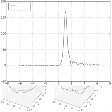
Figure 4: The unperturbed orbit lies flat along the $\mathbf{e}_{1}-\mathbf{e}_{2}$ plane. When $\alpha=0$, or when the electric field is constant in time, the orbit slants. When $\alpha\rightarrow\infty$, more waves are observed.

III.4 Orbit Equations and Limiting Conditions

To convert Eqs. (III.3) and (III.3) into rectangular coordinates, we use the expansions in Eq. (15a) and (15b), together with the identity $\mathbf{e}_{1}i\mathbf{e}_{3}=\mathbf{e}_{2}$ to arrive at

$$x =r_{0}\cos(\omega_{0}t+\varphi_{0}),$$ (53a)

$$y =r_{0}\sin(\omega_{0}t+\varphi_{0}),$$ (53b)

$$z =\frac{qE_{0}}{m\omega_{0}^{2}}\frac{1}{(\alpha^{2}-1)}(\cos(\alpha\omega_{0}t+\varphi)-\cos(\omega_{0}t+\varphi)),$$ (53c)

and

$$\dot{x} =-r_{0}\omega_{0}\sin(\omega_{0}t+\varphi_{0}),$$ (54a)

$$\dot{y} =r_{0}\omega_{0}\cos(\omega_{0}t+\varphi_{0}),$$ (54b)

$$\dot{z} =\frac{qE_{0}}{m\omega_{0}}\frac{1}{(\alpha^{2}-1)}(-\alpha\sin(\alpha\omega_{0}t+\varphi)+\sin(\omega_{0}t+\varphi)).$$ (54c)

Equations (53a) to (53c) are the equations for plotting the orbit of the electron as a function of time. Equations (54a) to (54c) are for plotting the corresponding velocities.

When the perturbing frequency $\omega=0$, corresponding to $\alpha=0$, the expressions for $z$ and $\dot{z}$ in Eqs. (53c) and (54c) reduces to

$$z =-\frac{qE_{0}}{m\omega_{0}^{2}}(\cos\varphi-\cos(\omega_{0}t+\varphi)),$$ (55a)

$$\dot{z} =-\frac{qE_{0}}{m\omega_{0}}\sin(\omega_{0}t+\varphi).$$ (55b)

If $\varphi=0$, the perturbing field is $\mathbf{E}=E_{0}\mathbf{e}_{3}$, so that

$$z =-\frac{qE_{0}}{m\omega_{0}^{2}}(1-\cos(\omega_{0}t)),$$ (56a)

$$\dot{z} =-\frac{qE_{0}}{m\omega_{0}}\sin(\omega_{0}t).$$ (56b)

On the other hand, if $\varphi=\pi$, the perturbing field is $\mathbf{E}=E_{0}\mathbf{e}_{3}$, so that

$$z =\frac{qE_{0}}{m\omega_{0}^{2}}(1+\cos(\omega_{0}t)),$$ (57a)

$$\dot{z} =\frac{qE_{0}}{m\omega_{0}}\sin(\omega_{0}t).$$ (57b)

These are the behavior of the electron’s orbit along the $z-$direction when the perturbing electric field is constant, also known as the DC electric field.

Now, when the perturbing frequency $\omega=\omega_{0}$, corresponding to $\alpha=1$, the field resonates with the electron’s orbit. The only terms affected are $z$ and $\dot{z}$ in Eqs. (53c) and (54c). Since both their numerators and denominators approach zero as $\alpha\rightarrow 1$, we apply L’hopital’s rule by differentiating the numerators and denominators prior to evaluation of the limits:

$$\lim_{\alpha\rightarrow 1}z =\frac{qE_{0}}{m\omega_{0}^{2}}\lim_{\alpha\rightarrow 1}\left(-\frac{\omega_{0}t\sin(\alpha\omega_{0}t)}{2\alpha}\right),$$ (58a)

$$\lim_{\alpha\rightarrow 1}\dot{z} =-\frac{qE_{0}}{m\omega_{0}}\lim_{\alpha\rightarrow 1}\left(\frac{\sin(\alpha\omega_{0}t+\varphi)}{2\alpha}\right)$$

$$\quad\ -\frac{qE_{0}}{m\omega_{0}}\lim_{\alpha\rightarrow 1}\left(\frac{\alpha\omega_{0}t\cos(\omega t+\varphi)}{2\alpha}\right).$$ (58b)

Hence,

$$\lim_{\alpha\rightarrow 1}z =-\frac{qE_{0}}{2m\omega_{0}}t\sin(\alpha\omega_{0}t),$$ (59a)

$$\lim_{\alpha\rightarrow 1}\dot{z} =-\frac{qE_{0}}{2m\omega_{0}}(\sin(\omega_{0}t+\varphi)+\omega_{0}t\cos(\omega_{0}t+\varphi)).$$ (59b)

Notice that the amplitude of the oscillations along $z$ and its corresponding velocity are linearly increasing in time. Once the amplitudes of the oscillations becomes so large, our perturbation approximations breaks down. Thus, our theory cannot really say what happens during ionization or whether ionization will really happen at all at the resonant frequency. (See Figs. 4 and 5)

\begin{overpic}[width=195.12767pt,tics=5,page=5]{rydberg_version2_graphics} \put(15.0,70.0){$\alpha=1$} \put(15.0,65.5){$\alpha=0.5$} \put(15.0,61.0){$\alpha=2$} \put(50.0,-5.0){$t$} \put(0.0,40.0){\makebox(0.0,0.0)[]{\rotatebox{90.0}{z}}} \end{overpic}

Figure 5: Height $z$ of the electron from its unperturbed circular orbit with respect to time.

IV Angular Momentum

IV.1 Product Form

Let us compute the product of the position $\mathbf{r}$ in Eq. (30) and its velocity $\dot{\mathbf{r}}$ in Eq. (31a):

$$\mathbf{r}\dot{\mathbf{r}}=(\mathbf{e}_{1}\hat{r}_{0}\hat{\psi}_{0}+\lambda\mathbf{e}_{3}\hat{s})(\mathbf{e}_{1}\hat{r}_{0}i\mathbf{e}_{3}\omega_{0}\hat{\psi}_{0}+\lambda\mathbf{e}_{3}\dot{\hat{s}}).$$ (60)

Distributing the terms, we get

$$\mathbf{r}\dot{\mathbf{r}} =\mathbf{e}_{1}\mathbf{e}_{1}\hat{r}_{0}^{*}\hat{\psi}_{0}^{*}\hat{r}_{0}i\mathbf{e}_{3}\omega_{0}\hat{\psi}_{0}$$

$$\quad\ +\mathbf{e}_{3}\mathbf{e}_{1}(\hat{s}\hat{r}_{0}i\mathbf{e}_{3}\omega_{0}\hat{\psi}_{0}-\dot{\hat{s}}\hat{r}_{0}^{*}\hat{\psi}_{0}^{*})+\mathbf{e}_{3}\mathbf{e}_{3}s\dot{\hat{s}},$$ (61)

after setting the perturbation parameter $\lambda=1$. Since $i=\mathbf{e}_{1}\mathbf{e}_{2}\mathbf{e}_{3}$ and $i\mathbf{e}_{3}=\mathbf{e}_{1}\mathbf{e}_{2}$, then Eq. (IV.1) reduces to

$$\mathbf{r}\dot{\mathbf{r}}=i\mathbf{e}_{3}\omega_{0}r_{0}^{2}-i\mathbf{e}_{1}s\hat{r}_{0}\omega_{0}\hat{\psi}_{0}-i\mathbf{e}_{2}s\hat{r}_{0}^{*}\hat{\psi}_{0}^{*}+\hat{s}\dot{\hat{s}}.$$ (62)

Separating the scalar and bivector parts of Eq. (62), we arrive at

$$\mathbf{r}\cdot\dot{\mathbf{r}} =\hat{s}\dot{\hat{s}},$$ (63a)

$$\mathbf{r}\times\dot{\mathbf{r}} =\mathbf{e}_{3}\omega_{0}r_{0}^{2}-\mathbf{e}_{1}s\hat{r}_{0}\omega_{0}\hat{\psi}_{0}-\mathbf{e}_{2}s\hat{r}_{0}^{*}\hat{\psi}_{0}^{*},$$ (63b)

after factoring out the trivector $i$ in the second equation.

Multiplying Eq. (63b) by the electron’s mass $m$ yields the the electron’s angular momentum:

$$\mathbf{L}=m\mathbf{r}\times\dot{\mathbf{r}}=\mathbf{e}_{3}\omega_{0}r_{0}^{2}-\mathbf{e}_{1}s\hat{r}_{0}\omega_{0}\hat{\psi}_{0}-\mathbf{e}_{2}s\hat{r}_{0}^{*}\hat{\psi}_{0}^{*},$$ (64)

where $s$ and $\dot{s}$ are the $\mathbf{e}_{3}$ components of the electron’s position $\mathbf{r}$ and velocity $\dot{\mathbf{r}}$ in Eqs. (III.3) and (III.3):

$$s =\frac{qE_{0}}{m\omega_{0}^{2}}\frac{1}{(\alpha^{2}-1)}(\cos(\alpha\omega_{0}t+\varphi)-\cos(\omega_{0}t+\varphi)),$$ (65a)

$$\dot{s} =\frac{qE_{0}}{m\omega_{0}}\frac{1}{(\alpha^{2}-1)}(-\alpha\sin(\alpha\omega_{0}t+\varphi)+\sin(\omega_{0}t+\varphi).$$ (65b)

Using the definitions $\hat{r}_{0}=r_{0}e^{i\mathbf{e}_{3}\varphi}$ and $\hat{\psi}_{0}=e^{i\mathbf{e}_{3}\omega_{0}t}$ in Eq. (64), and separating the $\mathbf{e}_{1}$, $\mathbf{e}_{2}$, and $\mathbf{e}_{3}$ components, we arrive at

$$L_{1} =-m\omega_{0}sr_{0}\cos(\omega_{0}t+\varphi_{0})-m\dot{s}r_{0}\sin(\omega_{0}t+\varphi_{0}),$$ (66a)

$$L_{2} =-m\omega_{0}sr_{0}\sin(\omega_{0}t+\varphi_{0})-m\dot{s}r_{0}\cos(\omega_{0}t+\varphi_{0}),$$ (66b)

$$L_{3} =m\omega_{0}r_{0}^{2},$$ (66c)

which are the parametric expressions for the angular momentum in rectangular coordinates.

IV.2 Harmonic Form

The vertical oscillation $s$ and its derivative $\dot{s}$ in Eqs. (65a) and (65b) may be expressed in exponential forms:

$$s =\frac{qE_{0}}{2m\omega_{0}^{2}}\frac{1}{(\alpha^{2}-1)}(e^{i\mathbf{e}_{3}(\alpha\omega_{0}t+\varphi)}+e^{-i\mathbf{e}_{3}(\alpha\omega_{0}t+\varphi)}$$

$$\qquad\qquad\qquad\quad-e^{i\mathbf{e}_{3}(\omega_{0}t+\varphi)}-e^{-i\mathbf{e}_{3}(\omega_{0}t+\varphi)}),$$ (67a)

$$\dot{s} =\frac{qE_{0}}{2m\omega_{0}}\frac{-i\mathbf{e}_{3}}{(\alpha^{2}-1)}(-\alpha e^{i\mathbf{e}_{3}(\alpha\omega_{0}t+\varphi)}+\alpha e^{-i\mathbf{e}_{3}(\alpha\omega_{0}t+\varphi)}$$

$$\qquad\qquad\qquad\quad\ +e^{i\mathbf{e}_{3}(\omega_{0}t+\varphi)}-e^{-i\mathbf{e}_{3}(\omega_{0}t+\varphi)}).$$ (67b)

These may be rewritten as

$$s =\frac{qE_{0}}{2m\omega_{0}^{2}}\frac{1}{(\alpha^{2}-1)}(\hat{\eta}\hat{\psi}_{0}^{\alpha}+\hat{\eta}^{*}\hat{\psi}_{0}^{-\alpha}$$

$$\qquad\qquad\qquad\qquad-\hat{\eta}\hat{\psi}_{0}-\hat{\eta}^{*}\hat{\psi}_{0}^{-1}),$$ (68a)

$$\dot{s} =\frac{qE_{0}}{2m\omega_{0}}\frac{-i\mathbf{e}_{3}}{(\alpha^{2}-1)}(-\alpha\hat{\eta}\hat{\psi}_{0}^{\alpha}+\alpha\hat{\eta}^{*}\hat{\psi}_{0}^{-\alpha}$$

$$\qquad\qquad\qquad\qquad+\hat{\eta}\hat{\psi}_{0}-\hat{\eta}^{*}\hat{\psi}_{0}^{-1}),$$ (68b)

where

$$\hat{\eta}=e^{i\mathbf{e}_{3}\varphi}.$$ (69)

Substituting Eqs. (68) and (68) back to Eq. (64) and noting that $\mathbf{e}_{2}i\mathbf{e}_{3}=-\mathbf{e}_{1}$, we obtain

$$\mathbf{L}=\mathbf{e}_{3}m\omega_{0}r_{0}^{2}-\mathbf{e}_{1}\frac{qE_{0}}{2\omega_{0}}\frac{1}{(\alpha^{2}-1)}\hat{\psi}_{L},$$ (70)

where

$$\hat{\psi}_{L} =\hat{\eta}\hat{r}_{0}\hat{\psi}_{0}^{\alpha+1}+\hat{\eta}^{*}\hat{r}_{0}\hat{\psi}_{0}^{-\alpha+1}-\hat{\eta}\hat{r}_{0}\hat{\psi}_{0}^{2}-\hat{\eta}^{*}\hat{r}_{0}$$

$$\quad\ -\alpha\hat{\eta}\hat{r}_{0}^{*}\hat{\psi}_{0}^{\alpha-1}+\alpha\hat{\eta}^{*}\hat{r}_{0}^{*}\hat{\psi}_{0}^{-\alpha-1}+\hat{\eta}\hat{r}_{0}^{*}-\hat{\eta}^{*}\hat{r}_{0}^{*}\hat{\psi}_{0}^{-2}.$$ (71)

Expanding the terms of $\hat{\psi}_{L}$ into exponential form, we get

$$\hat{\psi}_{L} =r_{0}(e^{i\mathbf{e}_{3}((\alpha+1)\omega_{0}t+\varphi+\varphi_{0})}+e^{i\mathbf{e}_{3}((-\alpha+1)\omega_{0}t-\varphi+\varphi_{0})}$$

$$\qquad-e^{i\mathbf{e}_{3}(2\omega_{0}t+\varphi+\varphi_{0})}-e^{i\mathbf{e}_{3}(-\varphi+\varphi_{0})}$$

$$\qquad\ -\,\alpha e^{i\mathbf{e}_{3}((\alpha-1)\omega_{0}t+\varphi-\varphi_{0})}+\alpha e^{i\mathbf{e}_{3}(-(\alpha+1)\omega_{0}t-\varphi-\varphi_{0})}$$

$$\qquad+e^{i\mathbf{e}_{3}(\varphi-\varphi_{0})}-e^{i\mathbf{e}_{3}(-2\omega_{0}t-\varphi-\varphi_{0})}),$$ (72)

Substituting the result back to Eq. (70) and separating the $\mathbf{e}_{1}$, $\mathbf{e}_{2}$, and $\mathbf{e}_{3}$ components, we arrive at

$$L_{1} =-\frac{qE_{0}r_{0}}{2\omega_{0}}\frac{1}{(\alpha^{2}-1)}\gamma_{1},$$ (73a)

$$L_{2} =-\frac{qE_{0}r_{0}}{2\omega_{0}}\frac{1}{(\alpha^{2}-1)}\gamma_{2},$$ (73b)

$$L_{3} =m\omega_{0}r_{0}^{2},$$ (73c)

where

$$\gamma_{1} =(1+\alpha)\cos((\alpha+1)\omega_{0}t+\varphi+\varphi_{0})$$

$$\quad+(1-\alpha)\cos((\alpha-1)\omega_{0}t+\varphi-\varphi_{0})$$

$$\quad\ -2\cos(2\omega_{0}t+\varphi+\varphi_{0}),$$ (74a)

$$\gamma_{2} =(1-\alpha)\sin((\alpha+1)\omega_{0}t+\varphi+\varphi_{0})$$

$$\quad-(1+\alpha)\sin((\alpha-1)\omega_{0}t+\varphi-\varphi_{0})$$

$$\quad\ +2\sin(\varphi-\varphi_{0}).$$ (74b)

Thus, since $\alpha=\omega/\omega_{0}$, we see that the orbit of the tip of the angular momentum vector $\mathbf{L}$ is a linear combination of circular motions with the following orbital frequencies:

$$\omega_{L}=\{\pm(\omega+\omega_{0}),\pm(\omega-\omega_{0}),\pm 2\omega_{0},0\}.$$ (75)

IV.3 Limiting Conditions

In the DC field limit, $\alpha\rightarrow 0$, so that

$$\lim_{\alpha\rightarrow 0}L_{1} =\frac{qE_{0}r_{0}}{2\omega_{0}}(\cos(\omega_{0}t+\varphi+\varphi_{0})$$

$$\qquad\qquad+\cos(-\omega_{0}t+\varphi-\varphi_{0})$$

$$\qquad\qquad-2\cos(2\omega_{0}t+\varphi+\varphi_{0})),$$ (76a)

$$\lim_{\alpha\rightarrow 0}L_{2} =\frac{qE_{0}r_{0}}{2\omega_{0}}(\sin(\omega_{0}t+\varphi+\varphi_{0})$$

$$\qquad\qquad-\sin(-\omega_{0}t+\varphi-\varphi_{0})$$

$$\qquad\qquad+2\sin(\varphi-\varphi_{0})).$$ (76b)

On the other hand, in the resonance frequency limit, $\alpha\rightarrow 1$, both the numerators and denominators of $L_{1}$ and $L_{2}$ approach zero, so that we apply the L’hopital’s rule:

$$\lim_{\alpha\rightarrow 0}L_{1} =-\frac{qE_{0}r_{0}}{4\omega_{0}}(\cos(2\omega_{0}t+\varphi+\varphi_{0})$$

$$\qquad-2\omega_{0}t\sin(2\omega_{0}t+\varphi+\varphi_{0})-\cos(\varphi-\varphi_{0})),$$ (77a)

$$\lim_{\alpha\rightarrow 0}L_{2} =-\frac{qE_{0}r_{0}}{4\omega_{0}}(-\sin(2\omega_{0}t+\varphi+\varphi_{0})$$

$$\qquad-\sin(\varphi-\varphi_{0})-2\omega_{0}t\cos(\varphi-\varphi_{0})).$$ (77b)

Notice that at the resonant frequency $\omega=\omega_{0}$, the $L_{1}$ and $L_{2}$ components of the angular momentum increases in time; in our perturbative approximation, the atom will be ionized.

V Power and Energy Absorption

V.1 Work-Energy Theorem

Figure 6: Projection of the tip of the angular momentum vector $\mathbf{L}$ in the $xy$ plane for different values of $\alpha$.

The work-energy theorem states that

$$\int_{\mathbf{r}_{0}}^{\mathbf{r}}\mathbf{F}\cdot d\mathbf{r}=\frac{1}{2}m{\mathbf{v}}^{2}-\frac{1}{2}m{\mathbf{v}_{0}}^{2}.$$ (78)

This may be rewritten as

$$\int_{0}^{t}P\,dt=\frac{1}{2}m{\mathbf{v}}^{2}-\frac{1}{2}m{\mathbf{v}_{0}}^{2},$$ (79)

where the power $P$ is defined as

$$P=\mathbf{F}\cdot\dot{\mathbf{r}}.$$ (80)

That is, the integral of the power $P$ expended by a force $\mathbf{F}$ acting to move a mass $m$ from time $t=0$ to $t$ is equal to the change in the mass’s kinetic energy between these times.

In our model, there are two forces acting on the electron: the Coulomb force $\mathbf{F}_{c}$ and the perturbing force $\mathbf{F}_{p}$. But since the sum of these two forces is $m\ddot{\mathbf{r}}$, as given in Eq. (28), then the left side of Eq. (79) becomes

$$P=m\ddot{\mathbf{r}}\cdot\dot{\mathbf{r}}.$$ (81)

We shall use this equation to compute the power absorbed by the atom.

V.2 Power: Product Form

To evaluate the left side of Eq. (81), we first multiply the expressions for $\ddot{\mathbf{r}}$ and $\dot{\mathbf{r}}$ in Eqs. (31b) and (31a):

$$\ddot{\mathbf{r}}\dot{\mathbf{r}}=(-\mathbf{e}_{1}\hat{r}_{0}\omega_{0}^{2}\hat{\psi}_{0}+\lambda\mathbf{e}_{3}\ddot{s})(\mathbf{e}_{1}\hat{r}_{0}i\mathbf{e}_{3}\omega_{0}\hat{\psi}_{0}+\lambda\mathbf{e}_{3}\dot{s})$$ (82)

Distributing the terms, we get

$$\ddot{\mathbf{r}}\dot{\mathbf{r}} =-\mathbf{e}_{1}\mathbf{e}_{1}\hat{r}_{0}^{*}\omega_{0}^{2}\hat{\psi}_{0}^{*}\hat{r}_{0}i\mathbf{e}_{3}\omega_{0}\hat{\psi}_{0}+\mathbf{e}_{3}\mathbf{e}_{1}\ddot{s}\hat{r}_{0}i\mathbf{e}_{3}\omega_{0}\hat{\psi}_{0}$$

$$\quad\ -\mathbf{e}_{1}\mathbf{e}_{3}\hat{r}_{0}\omega_{0}^{2}\hat{\psi}_{0}\dot{s}+\mathbf{e}_{3}\mathbf{e}_{3}\ddot{s}\dot{s},$$ (83)

after setting $\lambda=1$. Since $i=\mathbf{e}_{1}\mathbf{e}_{2}\mathbf{e}_{3}$ and $i\mathbf{e}_{3}=\mathbf{e}_{1}\mathbf{e}_{2}$, then Eq. (V.2) reduces to

$$\ddot{\mathbf{r}}\dot{\mathbf{r}}=-i\mathbf{e}_{3}r_{0}^{3}\omega_{0}^{3}-i\mathbf{e}_{1}\dot{s}\hat{r}_{0}\omega_{0}\hat{\psi}_{0}+i\mathbf{e}_{2}\dot{s}\hat{r}_{0}\omega_{0}^{2}\hat{\psi}_{0}+\ddot{s}\dot{s}.$$ (84)

Separating the scalar and bivector parts, we get

$$\ddot{\mathbf{r}}\cdot\dot{\mathbf{r}} =\ddot{s}\dot{s},$$ (85a)

$$\ddot{\mathbf{r}}\times\dot{\mathbf{r}} =-\mathbf{e}_{3}r_{0}^{3}\omega_{0}^{3}-\mathbf{e}_{1}\dot{s}\hat{r}_{0}\omega_{0}\hat{\psi}_{0}+\mathbf{e}_{2}\dot{s}\hat{r}_{0}\omega_{0}^{2}\hat{\psi}_{0},$$ (85b)

after factoring out $i$ in the second equation.

Equation (85a) leads to a very simple expression for the power absorbed by the atom:

$$P=m\ddot{\mathbf{r}}\cdot\dot{\mathbf{r}}=m\ddot{s}\dot{s}.$$ (86)

Taking the time derivative of $\dot{s}$ in Eq. (65b),

$$\ddot{s}=\frac{qE_{0}}{m}\frac{1}{(\alpha^{2}-1)}(-\alpha^{2}\cos(\alpha\omega_{0}t+\varphi)+\cos(\omega_{0}t+\varphi)),$$ (87)

and substituting this and that of $\dot{s}$ to Eq. (86), we get

$$P =\frac{q^{2}E_{0}^{2}}{2m\omega_{0}^{2}}\frac{1}{(\alpha^{2}-1)^{2}}\times$$

$$\qquad(-\alpha^{2}\cos(\alpha\omega_{0}t+\varphi)+\cos(\omega_{0}t+\varphi))\times$$

$$\qquad(-\alpha\sin(\alpha\omega_{0}t+\varphi)+\sin(\omega_{0}t+\varphi)).$$ (88)

We can show that this is equivalent to

$$P =\frac{q^{2}E_{0}^{2}}{2m\omega_{0}}\frac{1}{(\alpha^{2}-1)^{2}}\left(\alpha^{3}\sin(2\alpha\omega_{0}t+2\varphi)\right.$$

$$\qquad\qquad\left.-(\alpha^{2}+\alpha)\sin((\alpha+1)\omega_{0}t+2\varphi)\right.$$

$$\qquad\qquad+\left.(\alpha^{2}-\alpha)\sin((\alpha-1)\omega_{0}t)\right.$$

$$\qquad\qquad+\left.+\sin(2\omega_{0}t+2\varphi)\right),$$ (89)

which is the desired harmonic form of the power $P$ absorbed by the atom. Notice that power is not constant but fluctuating in time.

V.3 Average Power over Perturbing Period

\begin{overpic}[width=216.81pt,tics=5,page=7]{rydberg_version2_graphics} \put(18.0,70.0){$\langle P\rangle_{\tau}$} \put(50.0,-3.0){$\alpha$} \put(-1.0,40.0){\makebox(0.0,0.0)[]{\rotatebox{90.0}{$\langle P\rangle$}}} \end{overpic}

Figure 7: This is the graph of the average power over the perturbing period

Let us define the average power over the perturbing period as

$$\langle P\rangle_{\tau}=\frac{1}{\tau}\int_{0}^{\tau}P\,dt,$$ (90)

where

$$\tau=\frac{2\pi}{\omega}=\frac{2\pi}{\alpha\omega_{0}}.$$ (91)

Now, let us take the time average of the power $P$ in Eq. (V.4) over the perturbing period:

$$\langle P\rangle_{\tau} =\frac{q^{2}E_{0}^{2}}{2m\omega_{0}}\frac{1}{(\alpha^{2}-1)^{2}}\left(\alpha^{3}\langle\sin(2\alpha\omega_{0}t+2\varphi)\rangle_{\tau}\right.$$

$$\qquad\left.-(\alpha^{2}+\alpha)\langle\sin((\alpha+1)\omega_{0}t+2\varphi)\rangle_{\tau}\right.$$

$$\qquad+\left.(\alpha^{2}-\alpha)\langle\sin((\alpha-1)\omega_{0}t)\rangle_{\tau}\right.$$

$$\qquad\left.+\langle\sin(2\omega_{0}t+2\varphi)\rangle_{\tau}\right),$$ (92)

where

$$\langle\sin(2\alpha\omega_{0}t+2\varphi)\rangle_{\tau}$$

$$\qquad=0,$$ (93a)

$$\langle\sin((\alpha+1)\omega_{0}t+2\varphi)\rangle_{\tau}$$

$$\qquad=-\frac{1}{2\pi}\frac{\alpha}{(\alpha+1)}(\cos((1+1/\alpha)2\pi+2\varphi)-\cos(2\varphi))$$ (93b)

$$\langle\sin((\alpha-1)\omega_{0}t)\rangle_{\tau}$$

$$\qquad=-\frac{1}{2\pi}\frac{\alpha}{(\alpha-1)}(\cos((1-1/\alpha)2\pi)-1),$$ (93c)

$$\langle\sin(2\omega_{0}t+2\varphi)\rangle_{\tau}$$

$$\qquad=\frac{1}{2\pi}\alpha(\cos(4\pi/\alpha+2\varphi)-\cos(2\varphi)).$$ (93d)

Substituting these back to Eq. (V.4), we get

$$\langle P\rangle_{\tau} =\frac{q^{2}E_{0}^{2}}{4\pi m\omega_{0}}\frac{1}{(\alpha^{2}-1)^{2}}\times$$

$$\quad(-\alpha^{2}(\cos((1+1/\alpha)2\pi+2\varphi)-\cos(2\varphi))$$

$$\quad-\alpha^{2}(\cos((1-1/\alpha)2\pi)-1)$$

$$\quad+\alpha(\cos(4\pi/\alpha+2\varphi)-\cos(2\varphi)).$$ (94)

If $\varphi=0$, we have

$$\langle P\rangle_{\tau} =\frac{q^{2}E_{0}^{2}}{4\pi m\omega_{0}}\frac{1}{(\alpha^{2}-1)^{2}}\times$$

$$\quad(-\alpha^{2}(\cos((1+1/\alpha)2\pi)-1)$$

$$\quad-\alpha^{2}(\cos((1-1/\alpha)2\pi)-1)$$

$$\quad+\alpha(\cos(4\pi/\alpha)-1)).$$ (95)

Equation (V.3) is graphed in Fig. 7. Notice that despite the small oscillations in the interval $\alpha=0$ and $\alpha=1$, the power absorption curve is similar to that in Lorentz dispersion theory.

V.4 Average Power over Orbital Period

\begin{overpic}[width=216.81pt,tics=5,page=8]{rydberg_version2_graphics} \put(18.0,69.5){$\langle P\rangle_{\tau_{0}}$} \put(50.0,-3.0){$\alpha$} \put(-1.0,40.0){\makebox(0.0,0.0)[]{\rotatebox{90.0}{$\langle P\rangle$}}} \end{overpic}

Figure 8: This is the graph of the average power over the orbital period

Let us define the average power over the perturbing period as

$$\langle P\rangle_{\tau_{0}}=\frac{1}{\tau_{0}}\int_{0}^{\tau_{0}}P\,dt,$$ (96)

where

$$\tau_{0}=\frac{2\pi}{\omega_{0}}.$$ (97)

Now, let us take the time average of the power $P$ in Eq. (V.4) over the orbital period:

$$\langle P\rangle_{\tau_{0}} =\frac{q^{2}E_{0}^{2}}{2m\omega_{0}}\frac{1}{(\alpha^{2}-1)^{2}}(\alpha^{3}\langle\sin(2\alpha\omega_{0}t+2\varphi)\rangle_{\tau_{0}}$$

$$-(\alpha^{2}+\alpha)\langle\sin((\alpha+1)\omega_{0}t+2\varphi)\rangle_{\tau_{0}}$$

$$+(\alpha^{2}-\alpha)\langle\sin((\alpha-1)\omega_{0}t)\rangle_{\tau_{0}}$$

$$+\langle\sin(2\omega_{0}t+2\varphi)\rangle_{\tau_{0}}),$$ (98)

where

$$\langle\sin(2\alpha\omega_{0}t+2\varphi)\rangle_{\tau_{0}}$$

$$\qquad=-\frac{1}{2\pi}\frac{\cos(4\pi\alpha+2\varphi)-\cos(2\varphi)}{2\alpha},$$ (99a)

$$\langle\sin((\alpha+1)\omega_{0}t+2\varphi)\rangle_{\tau_{0}}$$

$$\qquad=-\frac{1}{2\pi}\frac{\cos(2\pi(\alpha+1))-\cos(2\varphi)}{\alpha+1},$$ (99b)

$$\langle\sin((\alpha-1)\omega_{0}t)\rangle_{\tau_{0}}$$

$$\qquad=-\frac{1}{2\pi}\frac{\cos(2\pi\alpha)-1}{(\alpha-1)},$$ (99c)

$$\langle\sin(2\omega_{0}t+2\varphi)\rangle_{\tau_{0}}$$

$$\qquad=0.$$ (99d)

Substituting these back to Eq. (V.4), we get

$$\langle P\rangle_{\tau_{0}} =\frac{q^{2}E_{0}^{2}}{8\pi m\omega_{0}}\frac{1}{(\alpha^{2}-1)^{2}}\times$$

$$\qquad\quad(-\alpha^{2}(\cos(4\pi\alpha+2\varphi)-\cos(2\varphi))$$

$$\qquad\quad-2\alpha(\cos(2\pi(\alpha+1))-\cos(2\varphi))$$

$$\qquad\quad-2\alpha(\cos(2\pi\alpha)-1)).$$ (100)

If $\varphi=0$, we have

$$\langle P\rangle_{\tau_{0}} =\frac{q^{2}E_{0}^{2}}{8\pi m\omega_{0}}\frac{-1}{(\alpha^{2}-1)^{2}}(\alpha^{2}(\cos(4\pi\alpha)-1)$$

$$-2\alpha(\cos(2\pi(\alpha+1))-1)-2\alpha(\cos(2\pi\alpha)-1)).$$ (101)

Equation (V.4) is graphed in Fig. 8. Notice that unlike in Fig. 7, there are periodic oscillations after $\alpha=2$.

VI Conclusion and Recommendation

We modelled the classical Hydrogen atom as an electron revolving in circular orbit around an immovable proton subject to the Coulomb force. We subjected this atom to a perturbing oscillating electric field perpendicular to the electron’s initial orbital plane. We showed that the resulting equations of motion of the electron along the axis of the perturbing electric field is similar to that of a simple harmonic oscillator with sinusoidal forcing. Furthermore, the absorbed energy averaged over the period of the perturbing field or over the orbital frequency of the electron is approximately similar to a resonance curve with one dominant frequency with finite peak at $\omega=\omega_{o}$; other small resonance peaks occur to the left or to the right of the major resonant frequency.

The Lorentz dispersion model of the light-atom interaction assumes that the electron is subject to Hooke’s force and the force due to the oscillating electric field of the light. Interestingly, even if our initial assumption is an electron in circular orbit around the nucleus, we still obtained the same forced harmonic oscillator equation as that of the standard model. We also obtained the same resonant frequency, though the actual peak is at a frequency slightly smaller than $\omega_{0}$. But what is new is that even though we did not put a damping term in our harmonic oscillator equation, we still obtained a finite energy absorption at the resonant frequency $\omega$. We also computed the electron’s angular momentum vector and showed that its tip traces rosette patterns similar to epicyclesGallavotti (2001).

In the future work, we shall extend our work to the interaction of the hydrogen atom with elliptically polarized radiation.

References

- Jackson (1975) J. Jackson, Classical Electrodynamics (Wiley, 1975).
- Zangwill (2013) A. Zangwill, Modern Electrodynamics (Cambridge University Press, 2013).
- Klein and Furtak (1986) M. Klein and T. Furtak, Optics (John Wiley and Sons, 1986).
- Akhmanov and Nikitin (1997) S. Akhmanov and S. Nikitin, Physical Optics (Oxford University Press, 1997).
- M.Born and Wolf (1964) M.Born and E. Wolf, Principles of Optics (Oxford University Press, 1964).
- Bayfield and Koch (1974) J. Bayfield and P. Koch, Physical Review Letters 33, 258 (1974).
- Haken and Wolf (2000) H. Haken and H. C. Wolf, The Physics of Atoms and Quanta: Introduction to Experiments and Theory (Springer-Verlag, 2000).
- Cole and Zou (2004) D. Cole and Y. Zou, Journal of Scientific Computing 21, 145 (2004).
- Brunello et al. (1996) A. Brunello, D. Farelly, and T. Uzer, Physical Review A 55, 3730 (1996).
- Farelly and Uzer (1995) D. Farelly and T. Uzer, Physical Review 74, 1720 (1995).
- Farelly and Griffiths (1992) D. Farelly and J. Griffiths, Physical Review A 45, R2678 (1992).
- Gajda et al. (1994) M. Gajda, B. Piraux, and K. Rzazweski, Physical Review A 50, 2528 (1994).
- Leopold and Percival (1978) J. Leopold and I. Percival, Physical Review Letters 41, 944 (1978).
- Grosfeld and Friedland (2002) E. Grosfeld and L. Friedland, Physical Review Letters E 65, 1 (2002).
- Neishtadt and Vasiliev (2005) A. Neishtadt and A. Vasiliev, Physical Review Letters E 71, 1 (2005).
- Sugon Jr. et al. (2008) Q. M. Sugon Jr., S. Bragais, and D. J. McNamara, Copernicus’s epicycles from newton’s gravitational force law via linear perturbation theory in geometric algebra (2008), eprint math/0807.2708v1.
- Vold (1993) T. Vold, Am. J. Phys. 61, 505 (1993).
- Hestenes (2003) D. Hestenes, Am. J. Phys. 71, 104 (2003).
- Sugon Jr. and McNamara (2004) Q. M. Sugon Jr. and D. J. McNamara, Am. J. Phys. 72, 104 (2004).
- Baylis (1996) W. E. Baylis, Clifford (Geometric) Algebras with Applications in Physics, Mathematics, and Engineering (Birkhäuser, 1996).
- Lounesto (2001) P. Lounesto, Clifford Algebra and Spinors (Cambridge University Press, 2001).
- Jancewicz (1989) B. Jancewicz, Multivectors and Clifford Algebras in Electrodynamics (World Scientific, 1989).
- Gallavotti (2001) G. Gallavotti, ATTI-Accademia Nazionale Dei Lincei Rendiconti Lincei Classe di Scienze Fisiche Matemaiche e Naturali Serie 9 Matematica e Applicazioni 12, 125 (2001).