TMD factorization and evolution at large $b_{T}$

Abstract:

In using transverse-momentum-dependent (TMD) parton densities and fragmentation functions, important non-perturbative information is at large transverse position $b_{T}$. This concerns both the TMD functions and their evolution. Fits to high energy data tend to predict too rapid evolution when extrapolated to low energies where larger values of $b_{T}$ dominate. I summarize a new analysis of the issues. It results in a proposal for much weaker $b_{T}$ dependence at large $b_{T}$ for the evolution kernel, while preserving the accuracy of the existing fits. The results are particularly important for using transverse-spin-dependent functions like the Sivers function.

1 Introduction

This talk summarized some recent work [1] in collaboration with Ted Rogers.

The overall motivation is to understand the evolution of transverse-momentum-dependent (TMD) parton densities (etc) especially at the relatively low values of $Q$ that have considerable current interest, as can be seen from many talks in this session on spin physics. We are particularly concerned with the non-perturbative part of the evolution, since there appear to be inconsistencies between the evolution found in fits [2, 3] to higher $Q$ Drell-Yan data, and the slower evolution preferred (e.g., [4, 5]) by more recent data at lower $Q$. When TMD functions are Fourier transformed into a space of transverse coordinates $\boldsymbol{b}_{\text{T}}$, non-perturbative contributions are at large $\boldsymbol{b}_{\text{T}}$.

Our aim was to to try to preserve good fits to the Drell-Yan data, while also agreeing with the lower energy data and satisfying non-perturbative constraints from the theory side.

2 Review of TMD factorization and the organization of non-perturbative information

We use the following TMD factorization formula for the Drell-Yan cross section differential in the lepton pair momentum $q^{\mu}$ and lepton angle:

$$\frac{\mathop{\mathrm{d}\mskip-0.59999mu\sigma}\nolimits}{\mathop{\mathrm{d}^{4}\mskip-0.59999muq}\nolimits\mathop{\mathrm{d}\mskip-0.59999mu\Omega}\nolimits}=\frac{2}{s}\sum_{j}\frac{\mathop{\mathrm{d}\mskip-0.59999mu\hat{\sigma}_{j\bar{\jmath}}}\nolimits(Q,\mu\mapsto Q)}{\mathop{\mathrm{d}\mskip-0.59999mu\Omega}\nolimits}\int e^{i\boldsymbol{q}_{\text{T}}\cdot\boldsymbol{b}_{\text{T}}}~{}\tilde{f}_{j/A}(x_{A},\boldsymbol{b}_{\text{T}};Q^{2},Q)~{}\tilde{f}_{\bar{\jmath}/B}(x_{B},\boldsymbol{b}_{\text{T}};Q^{2},Q)\mathop{\mathrm{d}^{2}\mskip-0.59999mu\boldsymbol{b}_{\text{T}}}\nolimits,$$ (1)

valid when $q_{\text{T}}\ll Q$ and polarization effects are ignored. The functions $\tilde{f}(x,\boldsymbol{b}_{\text{T}},Q^{2},Q)$ are the Fourier transformed parton densities (pdfs) to $\boldsymbol{b}_{\text{T}}$, with the CSS $\zeta$ and $\mu$ parameters set to $Q^{2}$ and $Q$. The perturbative hard scattering factor is $\mathop{\mathrm{d}\mskip-0.59999mu\hat{\sigma}}\nolimits(Q,\mu\mapsto Q)$. The TMD pdfs obey an evolution equation of the form

$$\frac{\mathop{\mathrm{d}\mskip-0.59999mu\ln\tilde{f}_{f/H}(x,b_{\text{T}};Q^{2};Q)}\nolimits}{\mathop{\mathrm{d}\mskip-0.59999mu\ln Q}\nolimits}=\gamma(\alpha_{s}(Q))+\tilde{K}(b_{\text{T}};Q)=\gamma(\alpha_{s}(Q))-\int_{\mu_{b}}^{Q}\frac{\mathop{\mathrm{d}\mskip-0.59999mu\mu}\nolimits}{\mu}\gamma_{K}(\alpha_{s}(\mu))+\tilde{K}(b_{\text{T}};\mu_{b}).$$ (2)

The strongly universal function $\tilde{K}(b_{\text{T}};\mu)$ controls evolution of the shape of the TMD functions, and its behavior at large $b_{\text{T}}$ is the primary concern of our work. In the right-most part of (2), a renormalization-group transformation to scale $\mu_{b_{*}}\propto 1/b_{*}$ was applied to remove large logarithms.

Non-perturbative information is (a) in the values of the TMD pdfs and of $\tilde{K}$ at large $b_{\text{T}}$, and (b) from ordinary pdfs that appear in the OPE that gives the TMD pdfs at small $b_{\text{T}}$.

To separate non-perturbative contributions to evolution, we use the CSS method to write:

$$\frac{\mathop{\mathrm{d}\mskip-0.59999mu\ln\tilde{f}_{f/H}(x,b_{\text{T}};Q^{2};Q)}\nolimits}{\mathop{\mathrm{d}\mskip-0.59999mu\ln Q}\nolimits}=\gamma(\alpha_{s}(Q))-\int_{\mu_{b_{*}}}^{Q}\frac{\mathop{\mathrm{d}\mskip-0.59999mu\mu}\nolimits}{\mu}\gamma_{K}(\alpha_{s}(\mu))+\tilde{K}(b_{*};\mu_{b_{*}})-g_{K}(b_{\text{T}};b_{\rm max}),$$ (3)

where a smooth cutoff on the perturbative part is provided by $b_{*}={b_{\text{T}}}/{\sqrt{1+b_{\text{T}}^{2}/b_{\rm max}^{2}}}.$ Perturbative calculations give the first three terms on the right of (3), while fits to data are made for a parameterized form for $g_{K}(b_{\text{T}};b_{\rm max})$, which includes the non-perturbative large $b_{\text{T}}$ contributions.

The predictive power of this TMD factorization formalism beyond the calculable perturbative contributions is from two sources. First is the universality of pdfs between reactions. Second is the strong universality of $\tilde{K}$, i.e., its lack of dependence on the reaction, on the hadron and quark flavor, and on spin and $x$. The $Q$ dependence of $\tilde{K}$ is governed by the perturbative function $\gamma_{K}$, leaving non-perturbative dependence as a function of $b_{\text{T}}$ only.

Common choices of $b_{\rm max}$ are $0.5\,\mathrm{GeV^{-1}}$ and $1.5\,\mathrm{GeV^{-1}}$. Observe that if $b_{\rm max}$ is chosen to be too conservatively small, then fitting of $g_{K}$ to data includes reproducing the full $\tilde{K}(b_{\text{T}})$ in a region of $b_{\text{T}}$ that is still accessible to perturbative calculations.

3 Geography of evolution

$q_{\text{T}}$
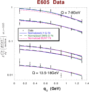
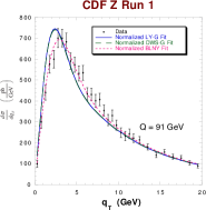
$b_{\text{T}}$
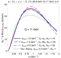
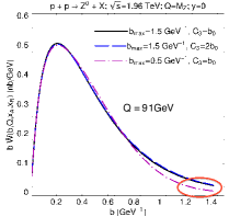
	$Q$: $7\mbox{--}18\,\mathrm{GeV}$, $\sqrt{s}=38.8\,\mathrm{GeV}$	$Q=m_{Z}$, $\sqrt{s}=1800\,\mathrm{GeV}$

Figure 1: Left, top: cross-section for $Q$ from $7\,\mathrm{GeV^{-1}}$ to $18\,\mathrm{GeV^{-1}}$ in the E605 experiment compared with fits by Landry et al. (BLNY), adapted from [2]. Left, bottom: corresponding $b_{\text{T}}$ integrand at $Q=11\,\mathrm{GeV^{-1}}$ for fits by Konychev and Nadolsky (KN) [3]. Right: similar plots for $Z$ production at the Tevatron; note that the cross section is for $\mathop{\mathrm{d}\mskip-0.59999mu\sigma}\nolimits/\mathop{\mathrm{d}\mskip-0.59999muq_{\text{T}}}\nolimits$ instead of $\mathop{\mathrm{d}\mskip-0.59999mu\sigma}\nolimits/\mathop{\mathrm{d}^{2}\mskip-0.59999mu\boldsymbol{q}_{\text{T}}}\nolimits$, which gives a kinematic zero at $q_{\text{T}}=0$.

As illustrated in Fig. 1, evolution to higher $Q$ shifts the dominant region of $b_{\text{T}}$ to ever lower values. Therefore the differential cross section as a function of $q_{\text{T}}$ broadens as $Q$ increases. The increasing suppression of the large $b_{\text{T}}$ region implies that the cross section is eventually dominated by perturbative effects, even at $q_{\text{T}}=0$, provided that the large distance properties are non-pathological.

4 Results for $\tilde{K}$ from fits

The evolution of the integrand $\tilde{W}$ in Eq. (1) is given by

$$\frac{\mathop{\mathrm{d}\mskip-0.59999mu\ln\tilde{W}}\nolimits}{\mathop{\mathrm{d}\mskip-0.59999mu\ln Q^{2}}\nolimits}=G(\alpha_{s}(Q))-\int_{\mu_{b_{*}}}^{Q}\frac{\mathop{\mathrm{d}\mskip-0.59999mu\mu}\nolimits}{\mu}\gamma_{K}(\alpha_{s}(\mu))+\tilde{K}(b_{*};\mu_{b_{*}})-g_{K}(b_{\text{T}};b_{\rm max}),$$ (4)

where $G(\alpha_{s}(Q))$ is perturbatively calculable. The right-hand side is the sum of a $Q$-dependent term and a $b_{\text{T}}$-dependent term. The $Q$-dependent term affects only the normalization of the cross section.

The change in shape of the cross section is governed only by the $b_{\text{T}}$-dependent part, which can be considered as the value of $\tilde{K}(b_{\text{T}};\mu_{1})$ at some fixed reference scale $\mu_{1}$:

$$\tilde{K}(b_{\text{T}};\mu_{1})=-\int_{\mu_{b_{*}}}^{\mu_{1}}\frac{\mathop{\mathrm{d}\mskip-0.59999mu\mu}\nolimits}{\mu}\gamma_{K}(\alpha_{s}(\mu))+\tilde{K}(b_{*};\mu_{b_{*}})-g_{K}(b_{\text{T}};b_{\rm max}).$$ (5)

Therefore we can gain an understanding of the change of shape of the $q_{\text{T}}$-dependent cross section with $Q$ from the functional dependence of $\tilde{K}(b_{\text{T}};\mu_{1})$ on $b_{\text{T}}$.

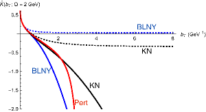
Typical $b_{\text{T}}$:	$0.5\,\mathrm{GeV^{-1}}$	$1.2\,\mathrm{GeV^{-1}}$	$3\,\mathrm{GeV^{-1}}$
$Q$:	$m_{Z}$	$10\,\mathrm{GeV}$	$2\,\mathrm{GeV}$

Figure 2: $\tilde{K}$ and its components from the KN and BLNY fits. See the text for details.

In Fig. 2 is shown the $b_{\text{T}}$ dependence of $\tilde{K}(b_{\text{T}};2\,\mathrm{GeV^{-1}})$ in the KN and BLNY fits. Overall, we see a decreasing function, which corresponds to the shift to smaller dominant values of $b_{\text{T}}$ with increasing $Q$ that we saw in Fig. 1.

The red curve gives the purely perturbative, renormalization-group-improved prediction for $\tilde{K}$. This is obtained by setting $b_{\rm max}=\infty$ and $g_{K}=0$ on the right-hand side of (5). The calculation shown was made with 2-loop approximations for the evolution of the running coupling and for $\gamma_{K}$. This prediction is valid when $b_{\text{T}}$ is small enough, but then diverges to $-\infty$ from the Landau pole in the approximated coupling, where perturbative-based calculations are completely untrustworthy.

CSS’s $\boldsymbol{b}_{*}$-prescription gives a smooth cut off of the perturbative term, intended to restrict it to a region where perturbatively based calculations are valid. The cut-off part of $\tilde{K}$, i.e., the first two terms on the right of (5) is shown as the dotted curves in Fig. 2. The blue curve is for $b_{\rm max}=0.5\,\mathrm{GeV^{-1}}$, corresponding to the BLNY fit of [2]. The black curve is for $b_{\rm max}=1.5\,\mathrm{GeV^{-1}}$, corresponding to the KN fit [3], which gives a better fit to the Drell-Yan data.

Finally we include the fitted functions $g_{K}$ for the two fits giving the black and blue solid curves. In both cases $g_{K}$ is purely quadratic: $g_{K}\propto b_{\text{T}}^{2}$. We first notice that each of these two curves matches the purely perturbative red curve beyond where the $b_{\rm max}$ cut off is important. Indeed the KN curve gives a good match to above $2\,\mathrm{GeV^{-1}}=0.4\,\mathrm{fm}$, which is, a priori, a region of at best marginal applicability of perturbative methods. That the fits match a perturbative calculation suggests that the primary result of fitting the one parameter in each fit is to reproduce perturbation theory and then to extrapolate the result to large $b_{\text{T}}$ in a non-singular fashion.

At large $b_{\text{T}}$, there is a dramatic difference between the KN and BLNY curves. This is reflected in the factor of two difference between the corresponding integrands at the right-hand edge of the lower right plot in Fig. 1. But that large fractional difference is in a place where the integrands are small, and so has little effect on the quality of the fits.

To understand where the differences between the curves matter, we need to know the typical values of $b_{\text{T}}$ involved. These are given below the graph in Fig. 2, and we deduce that the fits were primarily sensitive to $b_{\text{T}}$ below about $2\,\mathrm{GeV^{-1}}$. The values at larger $b_{\text{T}}$ are only an extrapolation, which need not be correct. To probe larger values of $b_{\text{T}}$ experimentally, we need lower $Q$.

That the extrapolation is actually wrong is indicated phenomenologically by the results of Sun and Yuan [4]. At large-$b_{\text{T}}$, the fitted Gaussian for the TMD pdfs combined with evolution governed by a quadratic $g_{K}$ gives a $Q$-dependent Gaussian behavior for the integrand $\tilde{W}$:

$$\tilde{W}\sim\dots e^{-b_{\text{T}}^{2}[\text{coeff}(x)+\text{const}\ln(Q^{2}/Q_{0}^{2})]}=\dots e^{-b_{\text{T}}^{2}a(Q,x)}\qquad\mbox{(at large $b_{\text{T}}$)}.$$ (6)

At a value of $Q$ appropriate for data from HERMES and CLAS, the value of $a(Q,x)$ in this equation becomes negative when the BLNY fit is used; this gives a completely unphysical cross section. The KN fit (with $b_{\rm max}=1.5\,\mathrm{GeV^{-1}}=0.3\,\mathrm{fm}$) merely gives a value of $a(Q,x)$ much too low to agree with the data.

5 Improved large-$b_{\text{T}}$ properties

Phenomenologically, we have good standard fits to Drell-Yan data that determine $\tilde{K}$ for $b_{\text{T}}$ up to around $1.5\,\mathrm{GeV^{-1}}=0.3\,\mathrm{fm}$, but not much further. At lower $Q$, larger $b_{\text{T}}$ dominates, but the extrapolated evolution appears to be too strong to agree with data. Furthermore, from the theoretical side the Gaussian large-$b_{\text{T}}$ behavior of TMD functions is disfavored [6]. Instead, the expected behavior of Euclidean correlation functions is an exponential times a power:

$$\frac{1}{b_{\text{T}}^{p}}e^{-mb_{\text{T}}}.$$ (7)

That is a non-perturbative statement, with $m$ being the mass of a relevant state. (One could, of course, ask whether this expectation is really correct in a confining theory like QCD)

Supposing that the mass in the exponent is energy-independent suggests that $\tilde{K}(b_{\text{T}})$ goes to a constant as $b_{\text{T}}\to\infty$. The constant gives a $Q$-dependent change (presumably a decrease) to the normalization of TMD pdfs at large $b_{\text{T}}$, but does not affect the exponential itself.

We therefore proposed [1] a new parameterization for $g_{K}$:

$$g_{K}(b_{\text{T}};b_{\rm max})=g_{0}(b_{\rm max})\left(1-\exp\left[-\frac{C_{F}\alpha_{s}(\mu_{b_{*}})b_{\text{T}}^{2}}{\pi g_{0}(b_{\rm max})\,b_{\rm max}^{2}}\right]\right)\,,$$ (8)

where

$$g_{0}(b_{\rm max})=g_{0}({b_{\rm max}}_{,0})+\frac{2C_{F}}{\pi}\int_{C_{1}/{b_{\rm max}}_{,0}}^{C_{1}/b_{\rm max}}\frac{d\mu^{\prime}}{\mu^{\prime}}\alpha_{s}(\mu^{\prime})$$ (9)

is the value of $g_{K}$ at $b_{\text{T}}=\infty$. This is arranged to have the following properties:

• At moderate $b_{\text{T}}$ it is approximately quadratic, and the sum of $g_{K}$ and the cut-off $\tilde{K}(b_{*};\mu_{b_{*}})$ approximately agrees with perturbation theory.

• At large $b_{\text{T}}$, it goes to a constant.

• The constant is given $b_{\rm max}$ dependence to compensate (to leading order), the $b_{\rm max}$ dependence of the perturbative term: $\lim_{b_{\text{T}}\to\infty}\tilde{K}(b_{*};\mu_{b_{*}})=\tilde{K}(b_{\rm max};\mu_{b_{\rm max}})$.

• Only one free parameter is used.

As we well see, the result gives much reduced $b_{\rm max}$ dependence of evolution compared with standard parameterizations. The exact $\tilde{K}$ is a quantity in full QCD and therefore does not itself have any $b_{\rm max}$ dependence whatsoever. If a simple quadratic function is used and happens to be correct for $g_{K}$ at one value of $b_{\rm max}$, it cannot be valid for other values of $b_{\rm max}$; a different functional form is needed.

Of course, we do not imagine that our proposed formula (8) is exactly correct; we simply propose it as a starting guess from which further refinement is possible.

Figure 3: Results of new parameterization for $\tilde{K}$.

We have not yet used our new parameterization to perform comparisons or fits with data. To show that it is likely to give reasonable results, we show in Fig. 3 what it gives for $\tilde{K}$ for two values of $b_{\rm max}$, with the choice that $g_{0}=0.3$ when $b_{\rm max}=1.5\,\mathrm{GeV^{-1}}$. It gives reasonable agreement with the KN results in the region of $b_{\text{T}}$ where the KN fit was determined by Drell-Yan data. But the flattening of the curves at larger $b_{\text{T}}$ shows that the evolution of the shape of the distribution is slower at large $Q$, as is necessary to be compatible with data at lower energy.

Figure 4: $\tilde{W}$ with new parameterization, compared with KN version.

Finally, to measure the compatibility with the Drell-Yan data, Fig. 4 shows some results (from Nadolsky, Rogers and Wang) for the Fourier transform in (1), at $Q=20\,\mathrm{GeV}$, in comparison with the KN results for two values of $b_{\rm max}$.

6 Summary of results

We argue that $\tilde{K}$ goes to a constant at large $b_{\text{T}}$. This value should be measured, of course. We propose a new parameterization to interpolate between the constant at large $b_{\text{T}}$ and the known behavior at moderate $b_{\text{T}}$. It should give better agreement with data and general principles over a wide range of $Q$. Further refinement is possible, of course.

To facilitate comparison between different work, fits should be presented in terms of the full $\tilde{K}(b_{\text{T}})$, not just in terms of $g_{K}$.

In [1], we argued that the following function can give useful diagnostics:

$$A(b_{\text{T}})=-\frac{\partial}{\partial\ln b_{\text{T}}^{2}}\frac{\partial}{\partial\ln Q^{2}}\ln\tilde{W}(b_{\text{T}},Q,x_{A},x_{B})\stackrel{{\scriptstyle\textrm{CSS}}}{{=}}-\frac{\partial}{\partial\ln b_{\text{T}}^{2}}\tilde{K}(b_{\text{T}},\mu).$$ (10)

It controls evolution of shape of TMD functions, is scheme and scale independent, and is strongly universal.

Acknowledgment: This material is based upon work supported in part by the U.S. Department of Energy under Grant No. DE-SC0008745.

References

- [1] J. Collins and T. Rogers, Phys. Rev. D 91 (2015) 074020 [arXiv:1412.3820].
- [2] F. Landry, R. Brock, P.M. Nadolsky and C.P. Yuan, Phys. Rev. D 67 (2003) 073016 [hep-ph/0212159].
- [3] A.V. Konychev and P.M. Nadolsky, Phys. Lett. B 633 (2006) 710 [hep-ph/0506225].
- [4] P. Sun and F. Yuan, Phys. Rev. D 88 (2013) 114012 [arXiv:1308.5003].
- [5] C. A. Aidala, B. Field, L. P. Gamberg and T. C. Rogers, Phys. Rev. D 89 (2014) 9, 094002 [arXiv:1401.2654 [hep-ph]].
- [6] P. Schweitzer, M. Strikman and C. Weiss, JHEP 1301 (2013) 163 [arXiv:1210.1267 [hep-ph]].